Measuring the Impact of Data Protection Techniques on Data Utility: Evidence from the Survey of Consumer Finances
Arthur Kennickell
Federal Reserve Board
Julia Lane
NORC/University of Chicago
Opinions expressed in the paper are those of the authors and do not necessarily reflect the view of the Federal Reserve Board or NORC.
1. Introduction
Data collectors face a complex problem. Usually substantial sums of money--often public money--are expended to collect data for research and policy purposes. There is an assumed obligation to make those data as fully and freely available as possible. Moreover, data collectors often create elaborate structures to create high quality data. However, ethical and often legal considerations force the collectors to take some set of actions to limit the ability of data users to identify respondents. During a time of rapidly improving technology for data linkage, like the present, public data sets are potentially increasingly vulnerable to intrusions. The most natural response of the most benign data collector would be to alter the data and to do so progressively over time in ways that seem likely to limit the possibilities of intrusion. In the absence of guidance by subject-matter experts, there is no reason to think that such changes would be in any way optimal for analytical purposes.
Despite the fact that much empirical economic research is based on public-use data files, the debate on the impact of disclosure protection on data quality has largely been conducted among statisticians and computer scientists. Remarkably, economists have shown very little interest in this subject, which has potentially profound implications for research. Without input from such subject-matter experts, statistical agencies may make decisions that unnecessarily obstruct analysis. The impact can range from simply reducing the precision of parameter estimates to biasing results or, in the worst case, closing down entire areas of research.
The practical consequences of such unguided data alterations are often quite substantial. For example, if data changes driven by disclosure protection are broadened over time, the true precision (as opposed to the precision computed from straightforward use of altered data) of parameter estimates is reduced. Thus, economists might incorrectly conclude that an economic phenomenon like race or sex discrimination was no longer an issue, even though the result is purely as an artifact of disclosure limitation techniques. Similarly, biased coefficients could lead to incorrect evaluation of the benefits and costs of different policies. Even if distortions that are employed preserve the first moments of a distribution, the second, third and fourth moments of a distribution can be distorted. Moreover, some techniques that may relatively harmless in a static context, can be very harmful in a dynamic context. Despite the potential consequences, few, if any, statistical agencies inform researchers about the potential consequences of disclosure protection techniques on the quality of their analysis.
This paper examines the impact of the application of disclosure protection techniques on a survey that is heavily used by both economists and policy-makers: the Survey of Consumer Finances. It discusses different approaches to convey information about changes in data utility to subject matter experts. We begin by reviewing the current literature on definitions and measures of data utility.
2. Data Utility
2.1 Definitions
Developing a definition of data utility for disclosure-protected microdata is relatively straightforward conceptually, but much more difficult to implement in a meaningful way. The emerging consensus appears to be based around the utility of the data for inference. Duncan et al., 2001, for example, describe data utility as "a measure of the value of information to a legitimate data user".1 Karr et al (2005a) define data quality, which is the precursor to data utility, as "the capability of data to be used effectively, economically and rapidly to inform and evaluate decisions. Necessarily, DQ is multi-dimensional, going beyond record-level accuracy to include such factors as accessibility, relevance, timeliness, metadata, documentation, user capabilities and expectations, cost and context-specific domain knowledge".2 Karr et al (2005b) then define data utility as the ability to preserve the same inferences from released microdata as for the protected data. 3 Statistical agencies define the concept slightly less formally, although the basic concept is the same. For example the OMB definition of utility is the "usefulness of the information for the intended audience's anticipated purposes."4 Similarly, Haworth et al.2001, writing for the European statistical system, define utility as "the totality of features or characteristics of a product or service that bear on its ability to satisfy stated or implied needs of customers".5
Implementing this consensus is more difficult. As Duncan et al, 2001, point out, early measures of information loss (the opposite of data utility) for tabular data were quite primitive, and included the percentage of suppressed cells, the total number or number of categories suppressed. Domingo-Ferrer and Torra 20016 attempted to develop measures on the principle that user analyses (e.g. regressions, means, etc.) on released data and on the original data should yield the same or at least similar results. A similar approach has been taken by Winkler (2005)7 who defines a dataset as analytically valid if the following is approximately preserved (some conditions apply only to continuous variables): Means and covariances on a small set of subdomains; Marginal values for a few tabulations of the data. Winkler goes further in stating that a microdata file is analytically interesting if six variables on important subdomains are provided that can be validly analyzed.
2.2 Data Quality Metrics
Not surprisingly, given the conceptual discussion above, the different metrics that have been developed in the literature attempt to measure the amount of information loss associated with the use of the data. A few of the metrics are reviewed here, using the notation of the original authors..
Duncan, et al, 2001, focus in on the user's key parameters of interest, ![]() , and use the reciprocal of a Mean Square Error as their measure of utility:
, and use the reciprocal of a Mean Square Error as their measure of utility:
Where ![]() is the set of parameters of interest to the user, and the subscripts x and x
is the set of parameters of interest to the user, and the subscripts x and x![]() referring to the masked and unmasked data respectively. This approach has a number of advantages. First, the measure has a direct analogue with a measure of risk. Second, it penalizes large differences more than small. In addition, the metric is one that is familiar to
most statisticians, and it has intuitive appeal in that large numbers reflect high levels of utility, smaller number reflect lower measures. Finally, the metric is measured over the outcomes of interest to users - namely the set of parameters of interest. However, it has a number of disadvantages
as well. The most obvious is that it is not scale invariant, so that although it is straightforward to make comparisons across different types of disclosure techniques on the same set of analytical exercises, it is not straightforward to compare across different specifications. In addition, there
is no natural interpretation of the order of magnitude of the measure.
referring to the masked and unmasked data respectively. This approach has a number of advantages. First, the measure has a direct analogue with a measure of risk. Second, it penalizes large differences more than small. In addition, the metric is one that is familiar to
most statisticians, and it has intuitive appeal in that large numbers reflect high levels of utility, smaller number reflect lower measures. Finally, the metric is measured over the outcomes of interest to users - namely the set of parameters of interest. However, it has a number of disadvantages
as well. The most obvious is that it is not scale invariant, so that although it is straightforward to make comparisons across different types of disclosure techniques on the same set of analytical exercises, it is not straightforward to compare across different specifications. In addition, there
is no natural interpretation of the order of magnitude of the measure.
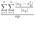
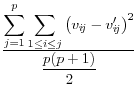
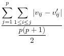
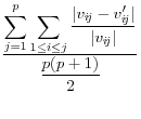
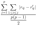
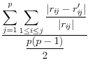
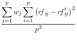
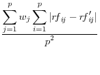
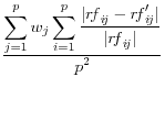
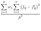
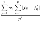
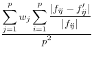
Domingo/Torra (2001) take a more catholic approach in listing a variety of summary statistics of the information in the released dataset (denoted by a prime) and the original dataset, such as the variance covariance matrices ![]() (on
(on ![]() and
and ![]() (on
(on ![]() , the correlation matrices
, the correlation matrices ![]() and
and ![]() , correlation matrices RF and RF' between the original variables and the principal components factors obtained through principal components analysis, the commonality between each of the original variables and the first principal component C and C'
8 and the factor score coefficient matrices
, correlation matrices RF and RF' between the original variables and the principal components factors obtained through principal components analysis, the commonality between each of the original variables and the first principal component C and C'
8 and the factor score coefficient matrices ![]() and
and
![]() .9 The summary statistics are listed in Table 1,
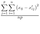
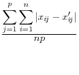
and include the mean square error, the mean absolute error, and the mean variation of each of these measures.
.9 The summary statistics are listed in Table 1,
and include the mean square error, the mean absolute error, and the mean variation of each of these measures.
| Mean square error | Mean abs. error | Mean variation | |
|---|---|---|---|
 |
 |
 |
|
 |
 |
 |
|
 |
 |
 |
|
 |
 |
 |
|
 |
 |
 |
|
 |
 |
 |
These approaches have a different type of appeal The advantage is that they summarize the differences between the disclosure-proofed and original input data, rather than on a set of parameters that may be very different for different groups of users. The metrics on which at least some of them are measured, like the correlations, are scale invariant. They are also all based on approaches that are familiar to statisticians. However, a major disadvantage is that the information that is included is likely to be too much to permit users to discriminate across disclosure protection approaches. For example, some datasets, like the National Longitudinal Surveys of Youth, or the Survey of Consumer Finances, have literally thousands of variables and while some are much more important than others, the metrics weight each input variable equally.
An alternative approach, which has not been suggested in the literature, but is certainly intuitively appealing, is to simply report the percent difference in key input variables and in parameter estimates. This has the twin advantages of being scale invariant and easily understood; the disadvantage is that percent differences are not standard statistical measures with well defined properties.
In any event, none of these summary statistics has been widely adopted, leaving researchers in the dark about the impact of disclosure protections on the quality of their analysis. For example, the most recent version of ![]() Argus, the microdata protection package produced by the CASC project, devotes only one paragraph to measuring the impact of disclosure protection techniques on data quality:
Argus, the microdata protection package produced by the CASC project, devotes only one paragraph to measuring the impact of disclosure protection techniques on data quality:
"In case of applying local suppressions only,
-ARGUS simply counts the number of local suppressions. The more suppressions the higher the information loss. In case of automatic global recoding
-ARGUS uses an information loss measure that uses the following parameters: a valuation of the importance of an identifying variable (according to the data protector), as well as a valuation of each of the possible predefined codings for each identifying variable."
P 43,
-Argus Manual 4.0, December 2004
Similarly, the Census Bureau's review of disclosure protection protocols, while providing an exhaustive list of ways to protect microdata, does not provide the impact on data utility. 10
3. Description of Survey of Consumer Finances and typical uses of data
The SCF has been conducted every three years by the FRB with the cooperation of the Statistics of Income Division (SOI) of the Internal Revenue Service since 1983. NORC has performed the data collection since 1992. This computer-assisted-personal interviewing (CAPI) survey collects data from a nationally representative sample of American households using a dual-frame sample design. One part is a multi-stage area-probability sample selected from the NORC National Frame. The other part, which is selected using statistical records derived from tax returns, is stratified to over-sample wealthy households.11 The data are used to examine cross-sectional variation as well as to evaluate trends over time. 12The survey gathers detailed data on households' balance sheets--their assets and liabilities--as well as collecting information on income, work, pensions, use of financial institutions, demographic characteristics and attitudes. Most of this information is commonly viewed as highly confidential by respondents. Thus, efforts to assure respondents of the measures taken to protect the confidentiality of their data play a central role in persuading them to participate in the survey and to provide reliable information. The pledge given to respondents becomes, at the very least, a moral obligation for the data collectors to take every effort to fulfill it. Furthermore, the data are collected under the framework of the Confidential Information Protection and Statistical Efficiency Act (CIPSEA) of 2002. Under this act, when respondents are told that their data are being collected "for statistical purposes only," as respondents in the SCF are told, there is also a strong legal obligation to ensure the protection of the confidentiality of the data collected. For the SCF, there is an additional obligation imposed by the use tax-derived data in the sample design. As a part of the agreement with SOI that makes the data available, the survey is obliged to develop and implement a plan for the release of micro data that passes a review by SOI staff.
The public version of the SCF, which is described in more detail below, is the only version of the data available outside the core project group at the FRB. Although it is possible for researchers within the Federal Reserve and at other institutions to request special estimates from the internal version of the data, the great majority of policy research and longer-term research is done with the public version of the data. Data users in many areas--taxation, saving, retirement, personal finance, more general finance, financial market regulation, and other areas--depend on the reliability of estimates obtained from the public data set. Thus, it is imperative that the actions taken to limit disclosure do not induce serious distortions of estimates obtained from this data set.
The necessity of alterations to the SCF data for purposes of disclosure limitation also stands in contrast to the strong push in the survey to produce high-quality data. Large amounts of resources are devoted to training and monitoring interviewers for purposes of quality control. For example, Athey and Kennickell (2005) describe a new procedure undertaken for the 2004 SCF to deal quickly with data quality issues during the field period of the survey.13 The survey also uses great care in data processing and documentation to ensure that the data are handled and described in a way that that would ultimately be most useful for research. For example, the survey documents the original content of every variable; it employs multiple imputation to provide a measurable basis for the amount of missing information, and it bases the imputation on a broad set of covariates to support a wide variety of multivariate analyses of the data.
4. Description of Disclosure Limitation Approaches
4.1 Generally used approaches
A number of different disclosure limitation techniques are used by statistical agencies: a good summary is provided by the Federal Committee on Statistical Confidentiality's Confidentiality and Data Access Committee.14The list of options is quite long. Some options can be categorized as the direct reduction of information - variable deletion, recoding variables into larger categories, rounding continuous variables using top and bottom coding, using local suppression and enlarging geographic areas.
Another set of options can be described as the perturbation of information: the microdata set is distorted prior to its publication. In this way, unique combinations of scores in the original data set may disappear and new unique combinations may appear in the perturbed data set; such confusion is beneficial for preserving statistical confidentiality. Examples of these include noise addition, data swapping, blanking and imputation, micro-aggregation, PRAM (post randomization Method of Perturbation) and the use of multiple imputation/modeling to generate synthetic data
4.2 Approach Used in Survey of Consumer Finances (including changes over time)
A number of different techniques are applied for purposes of disclosure limitation in the SCF.15 The most basic change made to the data set for public release is that some cases are deleted. If an observation is deleted if it has net worth greater than the level of the least wealthy person identified in the Forbes list of the wealthiest 400 people in the U.S.; there were three such cases in the 2004 SCF. The view supporting this alteration is that too much information is available that could be matched with the SCF to identify extremely wealthy.Some variables available in the internal version of the data are not released at all. Geographic information is generally recognized as being one of the most useful things to know in deducing the identity of a survey respondent. Absence of such information poses a particular problem for researchers who wish to exploit variation in institutional and other structures across states to identify important elements factors in statistical models of economic behavior. Variables related to the sample design, the administration of the interview, and a variety of other variables noted in detail in the SCF codebook are also suppressed.
Some categorical and other discrete variables are coarsened in the SCF public data set. For example, the detailed 4-digit occupation codes determined from verbatim responses from the respondents are reduced to one of six codes. For family members other than the household "head" and that person's spouse or partner, their ages are reduced to an indicator of whether they are aged 18 or older. For a number of other discrete variables, categories with small numbers of responses are combined with similar categories. Again, all such changes are documented in detail in the survey codebook.
Dollar variables in the SCF are all subjected to a type of rounding and the degree of rounding varies with the magnitude of the figure rounded. For example, values of a $1 million or more are rounded to the nearest $10,000 and values between $10,000 and $1 million are rounded to the nearest $1,000. To minimize systematic distortions, the data are rounded up or down with probability proportional to the value modulo the rounding value. That is, a value of $1,222,221 would be rounded to $1.23 million with probability 2,221/10,000 and to $1.22 million with probability 7,879/1000. A number of other variables are also rounded. For example, the size of a farm or ranch is rounded to the nearest 5 acres, the proportion of pension assets held in stocks is rounded to the nearest 5 percent, and the last year that the household filed for bankruptcy (it is has ever done so) is rounded to the nearest 3 years, an interval selected as appropriate for research purposes.
Top-coding and bottom-coding are used very sparingly. A decision to truncate the data in this way is usually made because the set of people affected is very small and very far removed from the rest of the distribution of households. For example, the number of checking accounts is top-coded at 10 and the age of the respondent is top-coded at 95. Negative values of certain income components and total income are bottom-coded at $-9.
The only other disclosure limitation procedure applied that has at least the potential for causing significant distortion of the data is a type of data simulation. This technique is applied to a set of cases selected systematically on the basis of their unusual values in terms of a set of characteristics and a random set of cases selected to assist in masking the primary set of cases. In the 2004 SCF, fewer than 350 cases were selected for this treatment. For the cases selected, the multiple imputation model developed for the SCF is used to simulate the values of all dollar variables; the values of all other variables are taken either as they were originally reported or as they were imputed in the final iteration of the iterative imputation routine. Even though the multiple imputation routines used for the simulations add a random error from the distribution of the unexplained variance of the variable simulated, because the sample size is relatively small one might still expect the cases selected for their unusual values to exhibit some regression toward the mean, and thus induce a serious distortion of the right tails of a number of distributions. Two factors help to mitigate this potential problem. First, the imputation model inputs tend to sustain some of the unusual qualities of cases. The imputation framework proceeds sequentially over variables, using as inputs covariances estimated using the final iteration of the imputed data and conditioning variables for the cases whose dollar values are to be simulated. All of the non-dollar-denominated conditional variables are taken from the final imputed data. The dollar values are intially taken from that data set as well, but once a value is simulated, the simulated value is used in later models in the sequence. Second, bounds are imposed on the outcomes of the simulations. These ranges are set as a baseline percent plus a randomized addition. The details of this process cannot be revealed, but the ranges are designed to provide a tight enough range to ensure that values cannot become too much larger or smaller, but also to allow sufficient range for the true values to be effectively disguised 16
To further complicate the task of a potential data intruder, other unspecified changes are made to the data. The number of such changes is relatively small and the changes are almost all of a sort that would be highly unlikely to affect any analysis that took account of the inherent sampling variability in the data.
Unlike the case of changes made to the data through coding, editing, and imputation, changes as a result of disclosure reduction procedures are not documented in the shadow variables available for every case and every variable. For example, a shadow variable for a simulated variable would be indistinguishable from that for an unaltered variable that had originally been imputed using range information.
The procedures described here have been in place since the 1989 SCF. However, changes have been made in a variety of the details of the application of the procedures. The main changes have been in the set of variables suppressed and the degree of coarsening applied to categorical and discrete variables. Care has been taken at every such step to ensure as much backward continuity of measurement as possible.
Finally, data users have been encouraged to give feedback when the disclosure limitation procedures have interfered with research. The overwhelmingly most common complaint has been the lack of geographic information noted above. Users might also be concerned about the distorting effects of the disclosure limitation procedures, but they would be unable to make a judgment about these effect with the data available to them. Among other things, this paper is intended provide such an evaluation.
5. Description of Impact on SCF Analysis
In this section we analyse the impact of the disclosure protection approach on the utility of some of the most commonly used SCF variables: income, individual net worth and the debt to income ratio, as well as the conditioning variable, age. We begin by applying the Duncan approach to comparing summary statistics derived from disclosure protected and original measures of net worth and debt to income; both overall and by income and age categories. We then describe the same differences in terms of percent change. We do the same exercise to summarize the impact of disclosure proofing on the results of a common regression. Finally, we summarize a subset of the Domingo/Torra statistics.
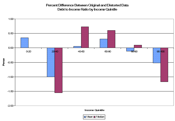
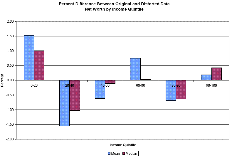
Table 1 presents the first set of measures for the mean and the median summary statistics, with the statistic calculated from the original data presented in the first column. The first interesting result is that the percent change in the statistic as a result of calculating the data from disclosure protected data, is quite small - less than 2% in all cases. The effects are also shown quite vividly in Figures 1 and 2. The second result is that the Duncan measure does capture the differences in consequences on data utility quite well: bigger numbers (reflecting higher utility) are consistently found where the percent errors are smaller. However, a major problem is that the Duncan measure is difficult to interpret. The measure for net worth is very small, reflecting the large scale of the variable; the measure on the debt to income ratio is very large, reflecting the variable's much smaller relative scale. As a result, making cross variable comparisons is difficult, as is making a determination of whether the loss in utility is "big" or "small".
We repeated the exercise for a standard regression analysis, and report the results in Table 2. A major concern with the application of the type of techniques used in disclosure proofing the SCF is that parameter estimates will be biased down, standard errors will be biased up, and the consequences will be that null hypotheses will wrongly fail to be rejected. A visual inspection of the parameter estimates derived from both the original and the disclosure proofed data suggests that these fears are substantially unfounded: both the parameter estimates and the standard errors are substantially unchanged after the application of the disclosure protection techniques. This is confirmed by examining the percent standard errors, which are reported in the next column. However, the Duncan measures are not particularly useful in conveying the information to current and prospective users of the public use data.
Finally, we calculated a subset of the Domingo/Torra metrics, but chose the one based on correlations matrices in view of the scale issues discussed above. We chose a data matrix of four variables: financial assets, non financial assets, debt and income. The MSE of the correlation matrix was effectively 0; the MAE was .05, while the MV was .13. This confirms that the effect of the disclosure protection on the quality of the input matrix was relatively minor.
| Variable:Statistic | Net Worth: Mean (Orig) | Net Worth: Mean (%diff) | Net Worth: Mean (Duncan) | Net Worth: Median (Orig) | Net Worth: Median (%diff) | Net Worth: Median (Duncan) | Debt To Income: Mean (Orig) | Debt To Income: Mean (%diff) | Debt To Income: Mean (Duncan) | Debt To Income: Median (Orig) | Debt To Income: Median (%diff) | Debt To Income: Median (Duncan) |
|---|---|---|---|---|---|---|---|---|---|---|---|---|
| All Incomes | 448230 | 0.05% | .00002 | 93098 | 0.1% | 0.0001 | 0.2011 | -0.03% | 307787011 | 0.1236 | 0% | NA |
| Income Quintile: 0-20 | 72620 | 1.53% | .00001 | 7496 | 1.01% | 0.00017 | 0.3115 | 0.36% | 816,027.4 | 0.0000 | 0.00% | NA |
| Income Quintile: 20-40 | 122037 | -1.55% | .0000 | 34348 | -1.02% | 0.00001 | 0.1664 | -1.00% | 361,589.2 | 0.0783 | -1.55% | 677,404 |
| Income Quintile: 40-60 | 193820 | -0.62% | .0000 | 71605 | -0.10% | 0.00018 | 0.1930 | 0.05% | 9,245,5621 | 0.1508 | 0.73% | 824,946 |
| Income Quintile: 60-80 | 342800 | 0.75% | .0000 | 159950 | 0.03% | 0.00040 | 0.1854 | 0.31% | 303,5122 | 0.1796 | 0.60% | 855,753 |
| Income Quintile: 80-90 | 485006 | -0.69% | .0000 | 311146 | -0.63% | 0.00000 | 0.1737 | -0.11% | 25,507,601 | 0.1728 | 0.10% | 35,856,431 |
| Income Quintile: 90-100 | 2534413 | 0.19% | .0000 | 924127 | 0.43% | 0.00000 | 0.1245 | -0.51% | 2,433,795 | 0.1117 | -1.17% | 586,292 |
| Original Data | Distorted Data | Percent Difference | Duncan | |
|---|---|---|---|---|
| Intercept | -11.9974
(.4336) |
-12.0347
(.4369) |
-0.31
-0.75 |
718
94,500 |
| Age | 0.1771
(.0166) |
0.1770
(.0168) |
0.04
-1.56 |
192,901,234
14,907,350 |
| Agesquared | -0.0931
(.0154) |
-0.0929
(.0157) |
0.21
-1.44 |
26,570,305
20,108,990 |
| Income | 1.5196
(.0266) |
1.5226
(.0269) |
-0.20
-1.33 |
107,076
8,025,102 |
6. Summary and Conclusion
The creation of public use datasets has been an important factor in advancing empirical social science research. National statistical institutes have rightly expended substantial energy to protecting the confidentiality of the respondents by using a variety of disclosure protection techniques. Recently, more attention has been paid to creating metrics that capture the impact of those techniques on data quality. This paper has demonstrated that those metrics, while possibly useful in summarizing the impact to the agencies themselves, are of limited use in conveying the information to researchers. Simpler measures, such as the percentage change in parameters from commonly used analytical work, might be more appropriate.
In further research, we intend to examine the impact of different types of protection techniques, such as topcoding and rounding, on data quality using these different metrics and using common estimation techniques.

