FRB: Finance and Economics Discussion Series: Screen Reader Version - The Yield Curve and Predicting Recessions

Skip to: [Printable Version (PDF)] [Bibliography] [Footnotes]

Finance and Economics Discussion Series: 2006-07 Screen Reader version*

The Yield Curve and Predicting Recessions

Jonathan H. Wright^*¹

Federal Reserve Board, Washington DC

February 2006

Keywords: Interest Rates, Forecasting, GDP Growth, Term Premiums, Probit.

Abstract: The slope of the Treasury yield curve has often been cited as a leading economic indicator, with inversion of the curve being thought of as a harbinger of a recession. In this paper, I consider a number of probit models using the yield curve to forecast recessions. Models that use both the level of the federal funds rate and the term spread give better in-sample fit, and better out-of-sample predictive performance, than models with the term spread alone. There is some evidence that controlling for a term premium proxy as well may also help. I discuss the implications of the current shape of the yield curve in the light of these results, and report results of some tests for structural stability and an evaluation of out-of-sample predictive performance.

JEL Classification: C22, E37, E43.

1. Introduction

The slope of the Treasury yield curve has often been cited as a leading economic indicator, with inversion of the curve being thought of as a harbinger of a recession. Of course, growth, recessions, and interest rates are all endogenous and any association among them is purely a reduced form correlation. However, historically, the three-month less ten-year term spread has exhibited a negative statistical relationship with real GDP growth over subsequent quarters, and a positive statistical relationship with the odds of a recession (see, for example, Estrella and Hardouvelis (1991) and Estrella and Mishkin (1996, 1998) and the references therein). The same is true for other similar measures of the difference between short- and long-term interest rates. The term spread is an important part of several indexes of widely followed leading indicators, including that of the Conference Board and the leading index and recession index of Stock and Watson (1989, 1993). The issue is quite topical because the yield curve is currently very flat, and actually modestly inverted between about one and five years.

The simplest theoretical rationale for why term spreads might be a useful leading indicator is that under the expectations hypothesis (neglecting term premiums), the term spread (short-term rates less long-term yields) measures the difference between current short-term interest rates and the average of expected future short-term interest rates over a relatively long horizon. The term spread is thus a measure of the stance of monetary policy (relative to long-run expectations). The higher is the term spread, the more restrictive is current monetary policy, and the more likely is a recession over the subsequent quarters.

Even with this rationale that neglects term premiums, it is not clear that the spread of short-term interest rates over the yield on a long-term bond should necessarily capture all the information in the yield curve about the likelihood of a recession. There is no fundamental reason why a rise in the level of current short-term interest rates must have the same predictive content for the likelihood of a recession as a fall in average expected future nominal interest rates over, say, the next ten years. But using the term spread as the sole explanatory variable has precisely this implication.

Moreover, neglecting term premiums seems inappropriate, as it is clear that term premiums exist, and are time-varying, and are typically increasing in the maturity of the bond, complicating the interpretation of spreads between short- and long-term Treasury yields. Hamilton and Kim (2002), and Ang, Piazzesi, and Wei (2006) have argued that the term premium and expectations hypothesis components of the term spread have quite different statistical correlations with future growth. This makes sense theoretically; an exogenous decline in the term premium, ceteris paribus, makes financial conditions more accommodative and so stimulates growth while flattening the yield curve. The federal funds rate is a measure of the stance of monetary policy that is less complicated by the effects of term premiums. More generally, the shape of the yield curve contains information about term premiums-in fact this is essentially the source of our ability to predict excess returns on longer-maturity bonds.

These considerations motivate asking if there is more information in the shape of the yield curve for future growth prospects than simply considering a term spread, such as the three-month over ten-year term spread. In this paper, I focus just on predicting recessions, rather than on the closely related question of growth forecasting. I consider a number of probit models for forecasting the binary variable that is one if there is an NBER recession in the subsequent quarters, and zero otherwise. The baseline model uses just the three-month over ten-year term spread. I then consider augmenting by the level of nominal federal funds rate, and some other yield curve variables including a term premium proxy, similar to the approach that Ang, Piazzesi and Wei (2006) found fruitful in the context of forecasting GDP growth. The probit regressions that include the federal funds rate and the three-month over ten-year term spread provide better in sample fit, and better out-of-sample predictive performance, than those regressions using the term spread alone. And, whereas the probit regression using the term spread alone currently predicts quite high odds of a recession, the probit regressions including the level of the federal funds rate do not.

The plan for the remainder of this paper is as follows. The data sources, alternative probit models, and prediction results are described in section 2. Structural stability is tested in section 3. Out-of-sample predictive performance is in section 4. Section 5 concludes.

2. Recession Prediction Using the Yield Curve: Alternative Probit Models

I consider four alternative models for probit regressions forecasting an NBER recession at some point in the next quarters. The first model, model A, is:

$\begin{displaymath} P(NBER_{t,t+h} =1)=\Phi (\tilde {\alpha }_0 +\tilde {\alpha }_1 SPREAD_t^{3M-10Y} ) \end{displaymath}$

(1)

where $NBER_{t,t+h}$ is the dummy that takes on a value 1 if and only if there is an NBER-defined recession at some point during quarters

through

, inclusive, $SPREAD_t^{3M-10Y}$ denotes the average three-month over ten-year constant maturity Treasury term spread² during quarter

and $\Phi (.)$ denotes the standard normal cumulative distribution function. Model B augments this with the level of the nominal federal funds rate:

$\begin{displaymath} P(NBER_{t,t+h} =1)=\Phi (\beta _0 +\beta _1 SPREAD_t^{3M-10Y} +\beta _2 FF_t ) \end{displaymath}$

(2)

where

denotes the average effective federal funds rate³ during quarter

. In principle, the real federal funds rate ought to be a better measure of the impetus or restraint to the economy implied by the stance of monetary policy. Model C uses both the nominal and real federal funds rates⁴ $^{ }$ in order to be able to test which of these measures of the stance of monetary policy actually has the best predictive power:

$\begin{displaymath} P(NBER_{t,t+h} =1)=\Phi (\delta _0 +\delta _1 SPREAD_t^{3M-10Y} +\delta _2 FF_t +\delta _3 RF_t ) \end{displaymath}$

(3)

where

denotes the real federal funds rate during quarter

, using the log difference in the core PCE price index over the previous four quarters as a proxy for expected inflation.

As argued above, the expectations hypothesis and term premium components of the slope of the yield curve may have quite different implications for future growth. Controlling for the level of the federal funds rate is at best an indirect way of accounting for this. Recently, Cochrane and Piazzesi (2005), building on work of Fama and Bliss (1987) and Campbell and Shiller (1991), find that a single linear combination of the term structure of forward rates has substantial predictive power for the excess returns from holding an -year bond for one year, over those from holding a one-year bond (for from 2 to 5). This "return forecasting factor" is a measure of the term premium on longer-term bonds. As a direct way to control for the different implications of the expectations hypothesis and term premium components of the yield curve, I consider using the term spread, the level of the funds rate, and Cochrane and Piazzesi's return forecasting factor as predictors of an NBER recession. This is model D, the specification for which is:

$\begin{displaymath} P(NBER_{t,t+h} =1)=\Phi (\gamma _0 +\gamma _1 SPREAD_t +\gamma _2 FF_t +\gamma _3 RFF_t ) \end{displaymath}$

(4)

where

is the return forecasting factor in quarter

estimated by a regression of the average excess returns from holding an

-year bond for one year, over those from on holding a one-year bond (averaged over

from 2 to 5) on the term structure of one-year forward rates at time

. To the extent that this is a noisy proxy for the term premium, it will of course introduce measurement error in the right-hand side variable. If the goal were estimation of a structural parameter, this would induce bias, but the task here is simply a reduced-form forecasting exercise.⁵

Each of the models is estimated using data from 1964Q1 to 2005Q4. The start date follows Fama and Bliss (1987), Ang, Piazzesi, and Wei (2006) and others. Some researchers have estimated regressions with data back as far as 1952, but data on long-term yields before 1964 may be unreliable because at that time there were very few long maturity bonds that did not have prices distorted by being either callable or "flower bonds" (redeemable at par in payment of estate taxes). The results are shown in Tables 1, 2 and 3 for horizons h=2, 4 and 6 quarters, respectively. The estimation method and construction of standard errors (taking account of the overlapping nature of the forecasts) are described in the appendix.

2.1 Results

Turning to the results, in model A, the coefficient on the three-month over ten-year term spread is statistically highly significant at all three horizons, reaffirming the underlying historical statistical association. In model B, both the federal funds rate and term spread are highly significant at all horizons. The fit of the regression, judging from the pseudo R-squared (which does not penalize model size) and the Bayes information criterion (which does penalize model size) is substantially better than using the term spread alone. In model C, where both the nominal and real funds rates are included, the model prefers the nominal funds rate and the real funds rate is not significant at any conventional significance level. In model D, the coefficient on the federal funds rate is once again significantly positive at each horizon. Meanwhile, the coefficient on the return forecasting factor is significantly negative at the six quarter horizon, but is not significant at shorter horizons. Judging from the Bayes Information Criterion, model B (using the term spread and the level of the funds rate alone) is the best fitting model at all horizons. I conclude that models that use both the level of the federal funds rate and the term spread give better in-sample fit than models with the term spread alone. There is some evidence that controlling for the return forecasting factor (term premium proxy) as well may help further.

2.2 A Few Historical Episodes and Current Implications

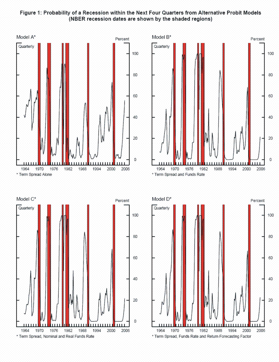
Figure 1 shows the fitted probabilities of a recession from models A, B, C, and D at the four-quarter-ahead horizon. NBER recessions are shown as the shaded regions. All of the models have generally quite good fit, with actual recessions following periods when the fitted probability of a recession was high. However, model A, which does not control for the level of the funds rate, predicted nearly even odds of a recession in 1995 and 1998, but no recession occurred in the subsequent four quarters. The other models, which do control for the level of the funds rate, predicted lower odds of a recession at those dates. Like today, 1995 and 1998 were episodes of flat yield curves where the level of the funds rate was not however especially high (though the funds rate was higher then than it is today). On the other hand, model A gave lower odds of a recession in the run-up to the 1990 recession than models that control for the level of the funds rate, and of course a recession did occur. The shape of the yield curve that has historically been the strongest predictor of recessions involves an inverted yield curve with a high level of the funds rate. Model A does not take this into account, while the other models do and these examples illustrate a few cases where that turned out to be right.

Not surprisingly, the models currently however have quite different implications. Model A now puts the odds of a recession in the next four quarters at over 50 percent. Models B, C, and D predict odds of a recession of around 20 percent, which is actually in the range of the unconditional probability of a recession in any four-quarter period. This more optimistic, and arguably more reasonable, prediction is consistent with the odds of a recession reported in the most recent Survey of Professional Forecasters (February 2006).

3. Structural Stability

Some authors have conjectured that the relationship between the yield curve and growth may have changed in recent years. Giacomini and Rossi (2005) and Estrella, Rodrigues, and Schich (2003) find evidence that the predictive power of the yield curve for growth has weakened since the 1980s. The latter paper however also tests for a structural break in the relationship between the term spread and a recession dummy and does not find a significant break.

Given the limited number of recessions in the United States over the last forty years, estimating a model allowing for all of the parameters to shift does not seem appropriate; the models as they stand are already quite richly parameterized. However, Lagrange multiplier tests for parameter stability require estimation of only the restricted model, without parameter breaks. These tests include the test of Nyblom (1989) and the sup-LM test of Andrews (1993) and are described in a bit more detail in the technical appendix. The structural stability test statistics are reported in Table 4 for models 1, 2, and 3 and horizons 2, 4, and 6. Neither test is significant, even at the 10 percent level, for any model or horizon. Consistent with the results of Estrella, Rodrigues, and Schich (2003), I find no evidence for a structural break in the relationship between different measures of the shape of the yield curve and the binary recession dummy.⁶ $^{ }$ Failure to reject a null hypothesis does not of course mean that it is true. Tests can have poor power, and I suspect that with the small number of recessions in this sample, the tests might fail to detect even quite notable parameter instability. The instability in the relationship between the yield curve and output growth underscores this possibility. Nevertheless, I do not have much evidence for time-variation in parameters in the association between yield curve variables and recessions.

4. Out-of-Sample Prediction of Recessions and Expansions

A stringent test of any forecast that guards against the danger of overfitting is to consider pseudo-out-of-sample predictive performance. For each model, and each horizon, I recursively compute predicted recession probabilities in each quarter, beginning with the forecast made in 1980Q1. I then consider the root mean square error of these predictions. That is, if $\hat {p}_t$ is the fitted probability of a recession between quarter and quarter , estimated using data available at time , then the root mean square prediction error is

$\begin{displaymath} RMSE_h =\sqrt {\frac{1}{T^\ast }\Sigma _{t=1}^{T^\ast } (\hat {p}_t -NBER_{t,t+h} )^2} \end{displaymath}$

(5)

where $T^\ast$ is the total number of pseudo-out-of-sample forecasts. The results are shown in Table 5. The forecasts from model B (which controls for the federal funds rate) and model D (which controls for the federal funds rate and the expected excess returns on long-term bonds) both dominate the forecasts from the baseline model A at all horizons. While the number of recessions is still too small to draw strong conclusions from this, it does not indicate that models B and D, which both control for the level of the federal funds rate in addition to the term spread, are overfitted.

5. Conclusions

Consistent with recent work by Ang, Piazzesi, and Wei (2005) on forecasting growth, I have found that there is more information in the shape of the yield curve about the likely odds of a recession than that provided by the term spread alone. Probit models forecasting recessions that use both the level of the federal funds rate and the term spread give better in-sample fit, and better out-of-sample predictive performance, than models with the term spread alone. There is some evidence that controlling in addition for Cochrane and Piazzesi's (2005) measure of expected excess returns on longer-maturity bonds may also help. The shape of the yield curve that has historically been the strongest predictor of recessions involves an inverted yield curve with a high level of the nominal funds rate. Currently, the yield curve is flat, not owing to a historically high level of the federal funds rate, but rather, to a low level of distant-horizon forward rates due in turn to some combination of low inflation expectations, low expected equilibrium real rates, and/or low term premiums. And a decline in term premiums seems to explain much of the fall in distant-horizon forward rates over the last couple of years, judging from multifactor term-structure models (Kim and Wright (2005)), or simply the comparison of the yield curve with survey-expectations for short-term interest rates at distant horizons. While a probit model using the term spread alone predicts high odds of a recession in the next four quarters, the other probit models that I estimate, which all control for the level of the funds rate, do not. This gives formal empirical support to a view that has been widely expressed by commentators that the present flatness of the yield curve is a reflection of low term premiums rather than especially tight monetary policy, and this flatness accordingly does not seem to herald a sharp slowdown.

In this regard, it is noteworthy that Australia, and especially the United Kingdom have had downward sloping yield curves for some time, apparently owing to low term premiums globally and to heavy special demand for longer duration assets from pension funds in the United Kingdom, rather than especially tight monetary policy. Both economies, however, have continued to expand robustly. Further analysis of the correlations between the shape of the yield curve and growth in foreign industrialized countries is an important topic that is left for future research.

Appendix: Construction of Standard Errors and Lagrange Multiplier Structural Stability Test Statistics

This appendix explains some of the econometric methods that I use in this paper for estimating a probit model with standard errors that are robust to serial correlation, and for constructing LM tests for structural stability in the probit model that are also robust to serial correlation. None of this is new, but the methods are not available in canned packages and are described here for completeness.

Each probit model that I estimate is of the form

$\begin{displaymath} y_t^\ast =\beta 'x_t +u_t \end{displaymath}$

$\begin{displaymath} y_t =1(y_t^\ast >0) \end{displaymath}$

where $\beta$ is a kx1 vector of parameters and

is standard normal. The model is estimated by maximum-likelihood using a sample of

observations. If

were i.i.d., then the log-likelihood function would be $l(\beta )=\Sigma _{t=1}^T l_t (\beta )$ where

$\begin{displaymath} l_t (\beta )=y_t \log (\Phi (\beta 'x_t ))+(1-y_t )\log (1-\Phi (\beta 'x_t )) \end{displaymath}$

I allow the

to be serially correlated, in recognition of the overlapping nature of the forecasts and so $l(\beta )$ is not in fact the log-likelihood, but is still the objective function that is being maximized, and is thus the pseudo-log-likelihood. Call the estimator that maximizes this objective function the pseudo-maximum-likelihood estimator, $\tilde {\beta }$ . Gourieroux, Montfort and Trongon (1982) and Poirier and Ruud (1988) show that this estimator is consistent under certain conditions which allow for quite general weak serial correlation, though rule out heteroskedasticity (most forms of heteroskedasticity would cause this pseudo-maximum-likelihood estimator to be inconsistent). The first order condition for the maximization of $l(\beta )$ is $\Sigma _{t=1}^T \frac{\partial l_t (\beta )}{\partial \beta }=0$ which yields a just-identified GMM estimator with the scores as the k moment conditions.

The general formula for the asymptotic variance of just-identified GMM applies in this context and thus $\sqrt T (\tilde {\beta }-\beta )\to _d N(0,H^{-1}VH^{-1})$ where

$\begin{displaymath} H=E[\frac{\partial ^2l_t (\beta )}{\partial \beta ^2}] \end{displaymath}$

and

$\begin{displaymath} V=\lim _{T\to \infty } Var(T^{-1/2}\Sigma _{t=1}^T \frac{\partial l_t (\beta )}{\partial \beta }) \end{displaymath}$

Letting

$\begin{displaymath} \hat {H}=T^{-1}\Sigma _{t=1}^T \frac{\partial ^2l_t (\tilde {\beta })}{\partial \beta ^2} \end{displaymath}$

and

$\begin{displaymath} \hat {V}=\Sigma _{j=-w}^w (1-\frac{w+1-\vert j\vert }{w+1})T^{-1}\Sigma _{t=1}^T \frac{\partial l_{t-j} (\beta )}{\partial \beta }\frac{\partial l_t (\beta )}{\partial \beta ^'} \end{displaymath}$

which is the usual Newey-West estimator with lag truncation parameter

, $\hat {H}^{-1}\hat {V}\hat {H}^{-1}$ gives an estimate of the asymptotic variance-covariance matrix of $\tilde {\beta }$ . See Estrella and Rodrigues (1998) for more discussion and some simulation evidence.

Turning to the tests for parameter constancy, the Nyblom (1989) LM test is given by

$\begin{displaymath} L=T^{-2}\Sigma _{t=1}^T m_t^' \hat {V}^{-1}m_t \end{displaymath}$

(see also Hansen (1990)), while the Andrews (1993) sup-LM test is

$\begin{displaymath} LM_{\sup } =\max _{\pi \in \Pi } \frac{1}{T\pi (1-\pi )}m_{[[\pi T]]}^' \hat {V}^{-1}m_{[[\pi T]]} \end{displaymath}$

where $m_t =\Sigma _{j=1}^t \partial l_t (\tilde {\beta })/\partial \beta '$ , [[.]] denotes the integer component of the argument and $\Pi$ is a closed subset of the unit interval excluding the endpoints, that is set to [0.15,0.85] in this paper. Both of these test statistics are functions of the partial sum process of the scores. Under the null hypothesis of no structural break, their asymptotic distributions are $\smallint _0^1 B_b (r)'B_b (r)dr$ and $\sup _{\pi \varepsilon \Pi } \frac{B_b (r)'B_b (r)}{r(1-r)}$ , respectively, where

is a k-dimensional standard Brownian bridge on the unit interval. Critical values of these limiting distributions are tabulated in the papers of Nyblom and Andrews.

Table 1: Probit Results for Forecasting NBER Recessions over the next two quarters
Model	A	B	C	D
Three Month less Ten-Year Spread	0.60 (3.96)	0.42 (2.84)	0.41 (2.64)	0.62 (1.34)
Federal Funds Rate		0.24 (3.05)	0.20 (2.03)	0.18 (1.06)
Real Federal Funds Rate			0.10 (0.91)
Excess Bond Return Forecasting Factor				0.07 (0.48)
Mc Fadden R-Squared	0.22	0.39	0.39	0.39
Bayes Information Criterion	-69.25	-58.11	-60.25	-60.51

Notes: This table shows the coefficient estimates, Mc Fadden R-squared and Bayes Information criterion from the maximum likelihood estimation of the probit regressions at a horizon of two quarters. Entries in parentheses are t-statistics, constructed using Newey-West standard errors. The sample is 1964Q1-2005Q4, as discussed in the text. The Bayes Information Criterion is $l-k\log (T)/2$ where is the maximized log-likelihood, is the number of parameters and is the sample size.

Table 2: Probit Results for Forecasting NBER Recessions over the next four quarters
Model	A	B	C	D
Three Month less Ten-Year Spread	0.74 (4.31)	0.76 (4.45)	0.76 (4.24)	0.55 (1.18)
Federal Funds Rate		0.35 (3.46)	0.36 (2.85)	0.43 (2.10)
Real Federal Funds Rate			-0.00 (-0.02)
Excess Bond Return Forecasting Factor				-0.07 (-0.48)
Mc Fadden R-Squared	0.29	0.50	0.50	0.50
Bayes Information Criterion	-73.18	-55.74	-58.29	-58.15

Notes: As for Table 1, except that the horizon is four quarters.

Table 3: Probit Results for Forecasting NBER Recessions over the next six quarters
Model	A	B	C	D
Three Month less Ten-Year Spread	0.75 (4.24)	0.81 (3.73)	0.84 (3.70)	0.07 (0.17)
Federal Funds Rate		0.36 (3.19)	0.39 (2.86)	0.66 (3.38)
Real Federal Funds Rate			-0.06 (-0.54)
Excess Bond Return Forecasting Factor				-0.29 (-2.03)
Mc Fadden R-Squared	0.29	0.48	0.48	0.50
Bayes Information Criterion	-78.48	-61.50	-63.83	-62.03

Notes: As for Table 1, except that the horizon is six quarters.

Table 4: Lagrange Multiplier Stability Test Statistics
Horizon	2 quarters	2 quarters		2 quarters	4 quarters	4 quarters		4 quarters	6 quarters	6 quarters		6 quarters
Model	A	B	C	D	A	B	C	D	A	B	C	D
Nyblom	0.23	0.44	0.51	0.49	0.26	0.46	0.55	0.51	0.27	0.42	0.48	0.62
Andrews	4.91	6.48	7.88	6.42	7.15	6.80	7.97	6.73	5.51	7.44	7.42	7.29

Notes: This table reports the Andrews and Nyblom Lagrange Multiplier tests for structural stability. None of these tests is significant, even at the 10 percent significance level.

Table 5: Out-of-Sample Root Mean Square Prediction Errors, 1980-2005Q4
Horizon	2 quarters	2 quarters		2 quarters	4 quarters	4 quarters		4 quarters	6 quarters	6 quarters		6 quarters
Model	A	B	C	D	A	B	C	D	A	B	C	D
	0.36	0.33	0.37	0.34	0.37	0.34	0.39	0.34	0.38	0.38	0.40	0.37

Notes: This table reports the root mean square error of the fitted recession probability as a predictor of the binary dummy that is 1 if and only if a recession subsequently occurred over three different subsamples.

Figure 1: The probability of a recession within the next four quarters as estimated by the models A-D is shown for each quarter. Quarters with a recession, as defined by the NBER business cycle dating committee, are shown by the shaded regions. (NBER recession dates are shown by the shaded regions)

References

Andrews, Donald W.K. (1993), "Tests for Parameter Instability and Structural Change With Unknown Change Point," Econometrica, 61, pp.821-856.

Ang, Andrew, Monika Piazzesi and Min Wei (2006), "What Does the Yield Curve Tell Us About GDP Growth?," Journal of Econometrics, forthcoming.

Campbell, John Y. and Robert J. Shiller (1991), "Yield Spreads and Interest Rate Movements: A Bird's Eye View," Review of Economic Studies, 58, pp.495-514.

Cochrane, John and Monika Piazzesi (2005), "Bond Risk Premia," American Economic

Review, 95, pp.138-160.

Efron, Bradley (1978), "Regression and ANOVA with Zero-One Data: Measures of Residual Variation," Journal of the American Statistical Association, 73, pp.113-121.

Estrella, Arturo and Gikas A. Hardouvelis (1991), "The Term Structure as Predictor of Real Economic Activity," Journal of Finance, 46, pp.555-576.

Estrella, Arturo and Frederic S. Mishkin (1996), "The Yield Curve as a Predictor of U.S. Recessions," Current Issues in Economics and Finance, 2.

Estrella, Arturo and Frederic S. Mishkin (1998), "Predicting U.S. Recessions: Financial Variables as Leading Indicators," Review of Economics and Statistics, 80, pp.45-61.

Estrella, Arturo and Anthony P. Rodrigues (1998), "Consistent Covariance Matrix Estimation in Probit Models with Autocorrelated Errors," Federal Reserve Bank of New York Staff Report 39.

Estrella, Arturo, Anthony P. Rodrigues and Sebastian Schich (2003), "How Stable is the Predictive Power of the Yield Curve: Evidence from Germany and the United States," Review of Economics and Statistics, 85, pp.629-644.

Fama, Eugene and Robert Bliss (1987), "The Information in Long-Maturity Forward Rates," American Economic Review, 77, pp.680-692.

Giacomini, Raffaella and Barbara Rossi (2005), "How Stable is the Forecasting Performance of the Yield Curve for Output Growth," mimeo, Duke University and University of California, Los Angeles.

Gourieroux, Christian, Alain Monfort and Alain Trognon (1982), "Estimation and Test in Probit Models with Serial Correlation", in J.P. Florens, M. Mouchart, J.P. Raoult and L. Simar (eds.), Alternative Approaches to Time Series Analysis, Publications des Facultés Universitaires Saint-Louis. Brussels.

Hamilton, James D. and Dong H. Kim (2002), "A Reexamination of the Predictability of Economic Activity Using the Yield Spread," Journal of Money, Credit and Banking, 34, pp.340-360.

Hansen, Bruce E. (1990), "Lagrange Multiplier Tests for Parameter Instability in Non-Linear Models," mimeo, University of Rochester.

Kim, Don and Jonathan H. Wright (2005), "An Arbitrage-Free Three-Factor Term Structure Model and the Recent Behavior of Long-Term Yields and Distant-Horizon Forward Rates," FEDS Paper, 2005-33.

Nyblom, Jukka (1989), "Testing for the Constancy of Parameters Over Time," Journal of the American Statistical Association, 84, pp.223-230.

Poirier, Dale J. and Paul A. Ruud (1988), "Probit with Dependent Observations," Review of Economic Studies, 55, pp.593-614.

Stock, James H. and Mark W. Watson (1989), "New Indexes of Coincident and Leading Economic Indicators," NBER Macroeconomics Annual.

Stock, James H. and Mark W. Watson (1993), "A Procedure for Predicting Recessions with Leading Indicators: Econometric Issues and Recent Experience," in J.H. Stock and M.W. Watson (eds.), New Research on Business Cycles, Indicators and Forecasting, University of Chicago Press, Chicago.

Footnotes

1. ^* Division of Monetary Affairs, Federal Reserve Board, Washington DC 20551. I am grateful to Mary Zaki for excellent research assistance and to Andy Levin and Jennifer Roush for helpful comments. All remaining errors are my own. The views expressed in this paper are solely the responsibility of the author and should not be interpreted as reflecting the views of the Board of Governors of the Federal Reserve System or of any other employee of the Federal Reserve System. Email addresses for the author is [email protected]. Return to Text

2. Source: H-15 release, Board of Governors of the Federal Reserve System. Return to Text

3. Source: H-15 release. Return to Text

4. Algebraically equivalent to augmenting model B with inflation. Return to Text

5. The return forecasting factor of Cochrane and Piazzesi (2005) has a high correlation with the term premium estimated from the three-factor term structure model estimated by Board staff (see Kim and Wright (2005)), but it has the advantage that it is easy to calculate back to the 1960s. Return to Text

6. I also conducted a Wald test for a break in the intercept alone in 1984Q1 in model B, as a hypothesis might be that the disinflation and the reduction in macroeconomic volatility that occurred around that time lowered both the frequency of recessions and the level of nominal interest rates, accounting for the correlation between the level of the federal funds rate and the likelihood of subsequent recessions. However, the hypothesis of a constant intercept was not rejected, and allowing for a break in the intercept at this date did not materially change the estimated coefficients on the term spread or the federal funds rate. Return to Text