
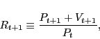
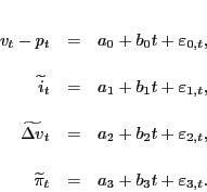
Federal Reserve Board
1 Introduction
According to the Flow of Funds Accounts of the United States, housing wealth accounted for about 40 percent of the overall net worth of households at the end of 2005. Housing's share of household net worth has increased more than 10 percentage points since the start of 1997, which we date as the beginning of the most recent housing boom. Unfortunately, there does not seem to be consensus among practitioners and housing economists about how to characterize the gains in house prices, either nationally or in any particular region. For example, a September 2005 report by economists at the Anderson School at UCLA concludes that house prices in California were overvalued by 45 percent. Gallin (2004) argues that housing may be overvalued because the nationwide rent-price ratio appears significantly lower than one would expect given historical statistical relationships among rents, house prices, and interest rates. Case and Shiller (2003) suggest that fundamentals may explain house prices in certain metro areas, but not in the more expensive cities of the East and West Coasts. In contrast, Himmelberg, Mayer, and Sinai (2005) argue that there is no evidence of a bubble in 2004 in any of the regional markets that they study, and McCarthy and Peach (2004) argue that there is no overvaluation at the national level.
In this paper, we use the dynamic Gordon growth framework of Campbell and Shiller (1988, 1989) to study housing valuations. The framework is an accounting identity based on the definition of one-period asset returns. It shows how the ratio of an asset's flow of fundamental value to its price can be decomposed into the expected present value of future growth rates of fundamentals, the expected present value of future interest rates, and the expected present value of future premia over those interest rates. Campbell and Shiller (1988, 1989), Campbell (1991), Campbell and Ammer (1993), and Shiller and Beltratti (1992) have successfully used this framework to study valuations in the stock and bond markets. In this paper, we extend this kind of analysis to the housing market by equating housing fundamentals with housing rents and housing valuations with the (log) rent-price ratio.
The dynamic Gordon growth framework provides a quantitative decomposition of housing market valuations that can be consistently compared across different geographic locations, across time within a single location, and across other asset markets. We estimate the real interest rate and real rent growth components using simple forecasting models; the housing premium is by definition the residual in the accounting identity.
While we are not the first to appeal to some form of the Gordon growth model in an analysis of housing markets (Cutts et al. 2005; Himmelberg, Mayer, and Sinai 2005), other studies assume that the housing premium is fixed across time, locations, or both. One of the major contributions of this paper is that we explicitly allow for housing premia to vary over time and by location. Specifically, we examine how movements in expected rent growth, interest rates, and housing premia account for both the trend and variability in housing valuations using semi-annual data over the 1975 to 2005 period. We conduct a separate analysis at the national and regional levels, and for twenty-three large metropolitan areas. Further, we examine how these relationships have changed over time by comparing the behavior of the components in the recent boom years, 1997 to 2005 to their behavior prior to 1997. We will show that time-varying housing premia are vital for understanding the behavior of housing valuations.
We find considerable variation in housing premia across both time and location. Average housing premia, expressed at an annual rate, range from less than 1 percent per year in Honolulu and New York City to about 3.5 percent per year in Denver and Philadelphia. Premia also exhibit substantial variation across time. At the national level, premia range from roughly 2.5 percent per year to less than 1 percent per year. Time-series variation in housing premia are even more extreme at the regional and metropolitan area levels.
Fundamentals - growth in rents - explain little of the trend and variance of rent-price ratios for all locations we study. This implies that the expected future real return to housing is the primary determinant of the trend and variance of rent-price ratios. In this way, the housing market is remarkably similar to the stock and bond markets.
We find that real interest rates and housing premia contribute about equally to the trend and variance of rent-price ratios. However, we also find that the relationship between real interest rates and housing premia has changed importantly since 1997. Before 1997, the estimated real rate and housing premium components were strongly negatively correlated: Changes to real rates were largely offset by opposite changes to housing premia. The negative correlation of real rates and housing premia resulted in rent-price ratios that were relatively insensitive to movements in real interest rates. Since 1997, however, changes to real interest rates and housing premia have been positively correlated. As a result, housing valuations appear to be more sensitive to changes in real interest rates in recent years.
Our results provide a new interpretation of the recent boom in house prices. We find that the recent run-up in house prices owes significantly to a decline in real interest rates and a decline in the housing premium. However, the predominant feature of the recent boom has been the change in the relationship between these two variables. Therefore, in our view, rent-price ratios in 2005 are considerably lower than could have been projected in 1997, even given advance knowledge of the decline in real interest rates that has occurred since 1997.
2 The Campbell-Shiller Decomposition
Consider the one-period gross return to housing:
![\displaystyle k+E_{t} [ \sum_{j=0}^{\infty }\rho^{j} r_{t+1+j}-\sum_{j=0}^{\infty }\rho ^{j}\Delta v_{t+1+j}]](img12.gif)
where lowercase letters represent logs of their uppercase counterparts,
or
![\begin{displaymath} v_{t}-p_{t} = k + E_{t} \sum_{j=0}^{\infty }\rho^{j} i_{t+1+j} +E_{t} \sum_{j=0}^{\infty }\rho^{j} \pi_{t+1+j} -E_{t} \sum_{j=0}^{\infty }\rho^{j} \Delta v_{t+1+j}], \end{displaymath}](img22.gif)
We refer to
The above representation of the (log) rent-price ratio in terms of future expected real interest rates, premia, and growth in real rents is a dynamic version of the classic Gordon growth model of asset prices in which the constant rent-price ratio is related to a constant real interest rate,
constant premium and constant growth rate of real rents,
![]() . The dynamic Gordon growth model above was first developed by Campbell and Shiller (1988, 1989) to analyze the determinants of dividend-price ratio variability.
Since then, it has been applied in the analysis of a variety of other markets. Shiller and Beltratti (1992) and Campbell and Ammer (1993), for example, use the dynamic Gordon growth model to decompose the variability of long-term bond yields. To implement the dynamic Gordon-growth model, in this
paper we use data on real interest rates to estimate the interest rate component of the rent-price ratio,
. The dynamic Gordon growth model above was first developed by Campbell and Shiller (1988, 1989) to analyze the determinants of dividend-price ratio variability.
Since then, it has been applied in the analysis of a variety of other markets. Shiller and Beltratti (1992) and Campbell and Ammer (1993), for example, use the dynamic Gordon growth model to decompose the variability of long-term bond yields. To implement the dynamic Gordon-growth model, in this
paper we use data on real interest rates to estimate the interest rate component of the rent-price ratio,
![]() , and data on real rent growth to estimate the rent-growth component,
, and data on real rent growth to estimate the rent-growth component,
![]() . Then, given data on rent-price ratios,
. Then, given data on rent-price ratios, ![]() , we use
the accounting identity above to identify the housing premium component,
, we use
the accounting identity above to identify the housing premium component,
![]() .
.
A popular alternative to equation (4) used by some authors to analyze housing valuations expresses the level of the rent-price ratio as
3 Data
All data in this study are at a semi-annual frequency and all of our calculations are appropriate for semi-annual data. In our tables and graphs, and throughout our analysis, however, we have annualized our data and results for expository purposes.
3.1 House Rent and Price Data
We assume that real rents represent the fundamental service flow from housing. Implicit rents on housing earned by owner-occupiers are unobserved and we therefore use data on rents paid by renters to impute rents accruing to owner-occupiers. Our source for nominal rents is the index for tenants' rent from the Bureau of Labor Statistics' (BLS) Consumer Price Index (CPI). We use information from the 2000 Decennial Censuses of Housing (DCH) to convert the CPI rent indexes to nominal dollar rents earned by owner-occupiers.1 To convert nominal rents to real rents, we deflate using the CPI excluding shelter. We use the BLS semi-annual rent index for the nation, four Census regions, and twenty-three separate metropolitan areas. The metropolitan areas used in this study are listed in Table 1. Column 1 of Table 1 lists the beginning sample date for each metropolitan area. The data for all metropolitan areas extends through the first half of 2005 (2005:H1).2 The national data span 1975:H1 to 2005:H1.3
In Figure 1, we graph real rental growth at annual rates for the nation and the four Census regions. Over the full sample, except in a few periods, annual real rental growth ranged between -2 percent and 2 percent. At the national level (top panel), real rents increased at a relatively quick pace during the mid-1980s, stagnated from 1986 to 1996, and increased again from 1996 to 2001. Since 2001, real rents have decelerated. Real rental growth in the four Census regions (bottom panel) looks quite similar to rental growth in the aggregate, and the average correlation between rent growth across the four regions is roughly 0.75.
We measure house-price changes using the weighted repeat-transactions house-price index published by the Office of Federal Housing Enterprise Oversight (OFHEO).4 The OFHEO index is based on price changes for owner-occupied homes that are resold or refinanced and therefore partially controls for changes in the composition of homes sold.5 We use the quarterly price index (converted to a semi-annual frequency) for the nation, the four Census regions, and the twenty-three metro areas for which we have rent data. As in the case of the rent data, the region-level price indexes are not weighted averages of the component cities in our analysis. OFHEO collects price data for over 300 metro areas and uses those data for regional and national estimates. Like our rent data, the national price data span 1975:H1 to 2005:H1; the regional and metro-area data begin at different dates but all end in 2005:H1.
The ratio of rents to prices (annual rate) for the nation and four regions are graphed in Figure 2. At the national level and across all four Census regions, the rent-price ratio was fairly flat from 1975 to about 1995, and then fell during the last decade of the sample. Nationally, the rent-price ratio declined from about 5.6 percent in 1975:H1 to 3.8 percent in 2005:H1. The South declined the least over the sample period (5.4 percent to 4.2 percent) while the West declined the most (4.8 percent to 2.8 percent).6 Also, while rent-price ratios vary considerably from period to period, they have declined since 2000 in every region and metropolitan area in our study (not graphed).
When taken together, figures 1 and 2 show that rent-price ratios vary more across regions than the growth rate of rents. Since real interest rates are roughly constant across geographic areas, and since rental growth rates in each region are very highly correlated, housing premia likely account for a substantial fraction of the variance in rent-price ratios.
3.2 Real Interest Rates
We use an estimate of the real expected yield on a 10-year U.S. Treasury bond as our real interest rate in the implementation of equation (4). As a result, our estimates of housing premia reflect the premium paid to housing over and above the yield on a 10-year Treasury. In principle, we could have chosen any real interest rate. We use the real 10-year Treasury as our real interest rate so our results are more comparable with other recent studies of housing valuations, such as Himmelberg et al. (2005), Cutts et al. (2005), Gallin (2004), and Meese and Wallace (1994).7 We constructed real interest rates using median inflation expectations from the Blue Chip Economic Indicator forecast from 1975:H1 through 1991:H1, and the median 10-year expected inflation forecasts from the Livingston survey from 1991:H2 to 2005:H1.
The nominal 10-year yield, 10-year expected inflation, and the real 10-year yield are plotted at annual rates in Figure 3. The nominal yield, expected inflation, and the real yield all increased prior to 1982, and have been declining since then. The real 10-year Treasury varies considerably in our sample. It increases from 2 percent at the start of our sample to about 8 percent in 1982, and then falls after that. At the end of the sample, the real 10-year Treasury yield is about 1.7 percent at an annual rate.
4 Time Variation in Housing Premia
A main goal of this analysis is to document the importance of time variation in the expected present value of housing premia,
![]() . However, all the empirical studies on housing that we know of assume a constant premium. So, a natural starting point for our analysis is to check that variation in
housing valuations can not be attributed to changes in real interest rates and rental growth rates alone.
. However, all the empirical studies on housing that we know of assume a constant premium. So, a natural starting point for our analysis is to check that variation in
housing valuations can not be attributed to changes in real interest rates and rental growth rates alone.
Consider the per-period approximate log premium,
| (6) |
The results show that housing premia are likely time-varying across most geographic locations for both time periods that we consider. In every Census region and at the national level, the null hypothesis of constant housing premia is rejected in the full sample and in each period. In some metro areas, the statistical evidence suggests that premia may not be time-varying in some periods. On the whole, however, the evidence against constant housing premia is remarkably strong. The results of the forecasting regression (not reported here) indicate that the rejection of constant housing premia arises because lagged house prices changes forecast future house prices changes, a well-known result documented by Case and Shiller (1989).
5 The Components of the Rent-Price Ratio
In this section we discuss our estimates of the expected present values of real rates,
![]() , real rent growth,
, real rent growth,
![]() , and ultimately housing premia,
, and ultimately housing premia,
![]() . To begin, recall that the expected present values depend on a discounting parameter,
. To begin, recall that the expected present values depend on a discounting parameter,
![]() . We use the first observation of the rent-price ratio in our sample to compute
. We use the first observation of the rent-price ratio in our sample to compute ![]() for each geographic area; column 3 of table 1 displays their values. We use the initial level of the rent-price ratio to fix
for each geographic area; column 3 of table 1 displays their values. We use the initial level of the rent-price ratio to fix ![]() (as opposed to the average
level over the sample period) to ensure that trends in house prices themselves do not influence our estimates.9 Note that areas with lower values for the rent-price ratio have
higher values for
(as opposed to the average
level over the sample period) to ensure that trends in house prices themselves do not influence our estimates.9 Note that areas with lower values for the rent-price ratio have
higher values for ![]() .
.
5.1 Estimating Discounted Expected Future Real Rates,

Our decomposition requires that for each period ![]() in our sample, we have estimates of the expected value of the entire future sequence of real interest rates from period
in our sample, we have estimates of the expected value of the entire future sequence of real interest rates from period ![]() forward. Campbell and Shiller (1989, 1989), Shiller and Beltratti (1992), and Campbell and Ammer (1993) use vector auto-regressive models to forecast future real rates. In this spirit, we use a simple
first-order auto-regressive model to forecast the expected present value of future real 10-year Treasury yields,
forward. Campbell and Shiller (1989, 1989), Shiller and Beltratti (1992), and Campbell and Ammer (1993) use vector auto-regressive models to forecast future real rates. In this spirit, we use a simple
first-order auto-regressive model to forecast the expected present value of future real 10-year Treasury yields,
| (7) |
Using these estimates of ![]() and
and ![]() , we construct the present
discounted value of future real interest rates as
, we construct the present
discounted value of future real interest rates as
| (8) | 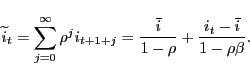 |
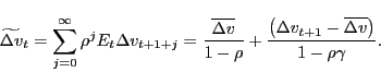
We plot
![]() and
and ![]() in figure 4 (for
in figure 4 (for ![]() ). The scaling puts
). The scaling puts
![]() on an annualized basis. Figure 4 shows that because
on an annualized basis. Figure 4 shows that because ![]() , the discounted present value of future real rates incompletely incorporates shocks to the current level of real rates, and therefore
, the discounted present value of future real rates incompletely incorporates shocks to the current level of real rates, and therefore
![]() is considerably smoother than
is considerably smoother than ![]() . Note that at the end of our
sample, the present discounted value of expected future real rates is roughly 3 percent while the real yield on the 10-year Treasury bond stands at roughly 1.7 percent.
. Note that at the end of our
sample, the present discounted value of expected future real rates is roughly 3 percent while the real yield on the 10-year Treasury bond stands at roughly 1.7 percent.
Obviously, if the dynamics of real interest rates are systematically different than those of the first-order auto-regressive model, our analysis will be inappropriate. In particular, our modeling framework assumes that real interest rates have a constant unconditional mean. This assumption is important in light of the rather low value of the real interest rate near the end of the sample period. If there has been a structural break in the level of the real 10-year Treasury, then our forecast model is mis-specified. We address this issue in the sensitivity analysis at the end of the paper.
5.2 Estimating Discounted Expected Future Real Rent Growth,

As with real interest rates, we use a simple first-order auto-regressive model to produce forecasts of the expected present value of future rent growth. Specifically, for each geographic area we estimate
| (9) |
The estimated parameters of the rental growth model are displayed in table 3. The table displays the average rate of real annual growth,
![]() , for each geographic area (column 1), the estimated annualized degree of persistence,
, for each geographic area (column 1), the estimated annualized degree of persistence, ![]() (column 2), the associated t-statistic (column 3), and the estimated standard deviation of real rental shocks,
(column 2), the associated t-statistic (column 3), and the estimated standard deviation of real rental shocks, ![]() (column 4).13 The average real growth rate of rents is smaller than 1 percent per year in most areas we consider (column 1). In addition, the persistence of rental growth rates is also
modest everywhere. Our data therefore suggest that although shocks to real rent growth can be quite large (column 4), these shocks are largely transitory, with a half-life of five quarters or less.
(column 4).13 The average real growth rate of rents is smaller than 1 percent per year in most areas we consider (column 1). In addition, the persistence of rental growth rates is also
modest everywhere. Our data therefore suggest that although shocks to real rent growth can be quite large (column 4), these shocks are largely transitory, with a half-life of five quarters or less.
5.3 Computing Discounted Expected Future Housing Premia,

Given
![]() and
and
![]() , we compute estimates of the discounted expected future value of housing premia,
, we compute estimates of the discounted expected future value of housing premia,
![]() , using the identity,
, using the identity,
| (11) |
for the nation, regions, and metro areas. Table 4 reports the average value of
The top panel of the first page of figure 5 displays
![]() the estimated housing premium at an annual rate at the national level.14Over much of the sample, the annualized premium ranges between 1 percent and 2 percent with three notable exceptions. Estimated premia are near 2.5 percent at the beginning of the sample, and below 1 percent in
the early 1980s and at the end of the sample. Premia at the national level have averaged roughly 1.6 percent over the entire sample (table 4, column 4). To give some perspective, one standard deviation of the national-level housing premium is
the estimated housing premium at an annual rate at the national level.14Over much of the sample, the annualized premium ranges between 1 percent and 2 percent with three notable exceptions. Estimated premia are near 2.5 percent at the beginning of the sample, and below 1 percent in
the early 1980s and at the end of the sample. Premia at the national level have averaged roughly 1.6 percent over the entire sample (table 4, column 4). To give some perspective, one standard deviation of the national-level housing premium is ![]() percentage point. All else equal, a one standard deviation increase in the national-level housing premium would imply a 10 percent decline in real house prices.
percentage point. All else equal, a one standard deviation increase in the national-level housing premium would imply a 10 percent decline in real house prices.
The data in table 4 and the plots of
![]() for the regions (figure 5, first page, bottom panel) show that the regional premia exhibit similar time-series patterns as the national premia. In
contrast, average estimated premia vary considerably across metro areas. For example, New York, Los Angeles, and San Francisco have average premia over the full sample below 1 percent, whereas Denver, Dallas, and Houston have average premia (over the full sample) in excess of 2.5 percent.
Note that not every city on the East and West coasts has low average housing premia. The average premium in Philadelphia is about 3 percent over the full sample, whereas the average premium in Milwaukee is 1.1 percent.
for the regions (figure 5, first page, bottom panel) show that the regional premia exhibit similar time-series patterns as the national premia. In
contrast, average estimated premia vary considerably across metro areas. For example, New York, Los Angeles, and San Francisco have average premia over the full sample below 1 percent, whereas Denver, Dallas, and Houston have average premia (over the full sample) in excess of 2.5 percent.
Note that not every city on the East and West coasts has low average housing premia. The average premium in Philadelphia is about 3 percent over the full sample, whereas the average premium in Milwaukee is 1.1 percent.
Estimated average premia have declined sharply in some metro areas between the two periods we consider. For example, average premia fell from 1.6 percent to 0.1 percent in Detroit, from 1.7 percent to 0.8 percent in Boston, and from 2.4 percent to 0.7 percent in Seattle. Importantly, the average housing premium appears to have declined in every metro area in our West Coast sample, as well as in Boston and New York, and in four of our Midwestern metro areas. However, the average premium paid to housing appears to have increased in Atlanta, Dallas, Houston, and Kansas City.
6.1 Decomposing Trends in Rent-Price Ratios
Figure 5 reveals a recent downward trend in the housing premia in many geographic areas. Indeed, estimated premia at the end of the sample are near all time lows for many areas. In this section, we attribute any trend in the (log) rent-price ratio to underlying trends in the real rate component,
![]() , rent growth component,
, rent growth component,
![]() , and the housing premium component,
, and the housing premium component,
![]() over the full, early, and late periods.
over the full, early, and late periods.
Consider the sample trend in the log rent-price ratio and its components,
The identity relating the components to the rent-price ratio in equation (4) implies that,
| (12) |
so that the trend in the (log) rent-price ratio over any period in time may be attributed to the trends in each of the individual components.
Table 5 presents estimates of this trend relationship for the full sample in columns 1-4, the early sample in columns 5-8, and the late sample in columns 9-12. The shares are defined as ![]() ,
, ![]() , and
, and ![]() . Over the full sample, the
rent-price ratio has trended down at the national level, in the four regions, and in most of our metro areas (column 1); Dallas, Houston, and Kansas City are the only exceptions. At the national level, roughly 40 percent of the decline in rent-price ratios is attributable to declining real
interest rates (column 2). Most of the rest of the trend decline is attributable to the downward trend in housing premia (column 4); trends in real rent growth are of minimal importance (column 3). By region, the rent-price ratio has fallen fastest in the Northeast and West, while the trend decline
in the Midwest and especially the South has been less pronounced. In the Midwest and West, nearly all of the decline in the log rent-price ratio is attributable to declining real rates, while in the Northeast only 67 percent of the trend in housing valuations is attributable to declining real
rates.15
. Over the full sample, the
rent-price ratio has trended down at the national level, in the four regions, and in most of our metro areas (column 1); Dallas, Houston, and Kansas City are the only exceptions. At the national level, roughly 40 percent of the decline in rent-price ratios is attributable to declining real
interest rates (column 2). Most of the rest of the trend decline is attributable to the downward trend in housing premia (column 4); trends in real rent growth are of minimal importance (column 3). By region, the rent-price ratio has fallen fastest in the Northeast and West, while the trend decline
in the Midwest and especially the South has been less pronounced. In the Midwest and West, nearly all of the decline in the log rent-price ratio is attributable to declining real rates, while in the Northeast only 67 percent of the trend in housing valuations is attributable to declining real
rates.15
Columns 5-12 highlight the fact that trends in housing valuations (rent-price ratios) reported over the full sample are largely reflective of changes to valuations since 1997. In the early sample, trend changes to housing valuations are, literally, all over the map. For example, the rent-price ratio declined in the Northeast and West, but increased in the South and to a lesser extent in the Midwest. Moreover, only the Northeast shows a significant trend decline in the rent-price ratio over this period.
Trends in housing valuations, real rates, and housing premia are much more pronounced in the late period (column 9). Rent-price ratios uniformly trended downward over this period. At the national level, the downward trend in real interest rates accounts for 38 percent of the trend decline in the rent-price ratio and the downward trend in housing premia accounts for 65 percent of the trend. In the Midwest and South, the trend in real rates accounts for more than two-thirds of the trend in housing valuations, but in the Northeast and West, the trend in real rates accounts for less than half of the trend decline in rent-price ratios. In metro areas such as Boston, Miami, Los Angeles, and San Francisco, declining premia account for over 70 percent of the trend in rent-price ratios, while in metro areas such as Chicago, Houston, Kansas City, Pittsburgh, and St. Louis, the trend in real rates accounts for over 70 percent of the trend decline in housing valuations.
6.2 Decomposing the Variability in Rent-Price Ratios
Figure 6 displays the decomposition of the log rent-price ratio for the nation as a whole. Note that we plot the sum of the log rent-price ratio and the constant of linearization and the negative of the real rent growth component. Thus, the three components sum to the total. In addition, we plot a vertical line in 1997.
By plotting all the components on one graph, several features become immediately apparent. First, the real rent growth component is less variable than the log rent-price ratio, implying that variation in fundamentals do not explain much of the variation in housing valuations. Second, the real interest rate and housing premium components are each more variable than the rent-price ratio itself, but they are negatively correlated, so that movements in one are largely offset by the other. Third, the negative correlation between the real rate and housing premium components appears to have weakened starting in 1997: Since 1997, both real rates and housing premia have trended down.
To address these features in a more systematic way, consider the following variance decomposition of the rent-price ratio,
| (13) | |||
We report the results from this variance decomposition over the full period in table 6a; table 6b presents the results of the variance decomposition over the early and late periods. In table 6a, column 1 lists the variance of the (log) rent-price ratio. Columns 2-4 report the share of the rent-price ratio's variance that owes to variance of
Considering the four Census regions, housing valuations are most volatile in the Northeast and West, and least volatile in the South (table 6a, column 1). This result is consistent with the finding that rent-price ratios have trended downward fastest in the Northeast and West and the least in the South over the full sample period. As figure 6 suggests, the rent-growth component explains very little of the variability in rent-price ratios (column 2). At the national level and in each of the four regions, variability in the rent growth component typically accounts for less than 10 percent of the variability in rent-price ratios. The finding that rent growth only accounts for a small share of the variability in housing valuations is consistent with the findings from other asset markets. In the case of the stock market, for example, Campbell and Ammer (1993) estimate that roughly 10 percent of the volatility of the dividend price ratio is accounted for by the volatility in dividends. In this way, houses behave like other financial assets.
Since rent growth volatility only accounts for a small portion of the volatility in rent-price ratios, the remainder of the volatility in rent-price ratios is accounted for by variability in real rates and premia. Columns 3 and 4 indicate that at the national and regional levels, the real rate and housing premium components account for more than 50 percent of the variation in rent-price ratios. In many cases these components are each more variable than rent-price ratios. But, the interest-rate and premium components are negatively correlated (column 7), so that movements in one component are largely offset by the other over the full sample.
The negative correlation of the components of housing returns highlights the fact that over the early sample, rent-price ratios were insensitive to changes in real interest rates. As an example, consider the case of the decline in the real interest rate component in the mid-1980's. From 1985:1 through 1990:1 the real interest rate component of house prices declined by 0.8 percentage point, from roughly 4.6 percent per year to 3.8 percent per year (figure 3). At the national level, the rent-price ratio only declined by 0.4 percentage point over this same period from, 5.2 percent to 4.8 percent (figure 2). Our accounting identity requires an increase in the housing premium of roughly 0.4 percentage point.16 The lack of responsiveness of rent-price ratios to movements in real interest rates over this period is a distinguishing feature of these data. More generally, over the full sample, movements in rent-price ratios typically reflected only a portion of the underlying movements in real interest rates, highlighted by the negative covariance in column 7.
The metro area results are similar. First, in nearly every metro area, the volatility of the rent growth component accounts for less than 10 percent of the volatility of the rent-price ratio and in only one case does it account for more than 15 percent of the volatility of the rent-price ratio. Second, both the real rate and housing premium components are highly variable and are negatively correlated with each other over the full sample. Accordingly, the lack of sensitivity of rent-price ratios to real rates is a widespread feature of these data that is apparent at the national, regional, and metro-area levels.
In table 6b we repeat the variance decomposition for the early and late periods; the table layout is similar to that of table 6a. The results in columns 1 and 8 show that, at the national level, there has been a large increase in the variability of rent-price ratios since 1997. Specifically, rent-price ratios have been more than four times as volatile, at the national level, during the late period than during the early period. This pattern however, is not shared across all regions. While the South and West have exhibited more volatile housing valuations over the later period, housing valuations in the Midwest and Northeast were about equally volatile over both periods. The results at the metro-area level are also mixed, with some areas, such as Minneapolis, Miami and San Diego, experiencing large increases in rent-price ratio variability while other metro areas including Boston, Detroit, Houston, and Portland experiencing sharp declines in the variation.
As in the case of the full sample, rent growth plays a minor role in accounting for the variability in rent-price ratios (columns 2 and 9). Indeed, the results suggest that the importance of rent growth has declined somewhat over time. Also, as in the case of the full sample, the insignificance of the rental-growth component implies that the real rate and housing premium components account for most of the variation of the rent-price ratio.
Table 6b highlights what we think is a key change in the relationship over time between the real rate and housing premium components. Over the early period, the covariance between the real rate and housing premium component is estimated to be negative at the national level, regional level, and in every metro area (column 7). Moreover, the size of the covariance is large. In nearly every case the estimated covariance between the real rate and premium component is estimated to be larger than the variance of the underlying rent-price ratio, indicating a strong tendency for movements in one component to be offset by the other. Over the late period, the picture is quite different. At the national, regional and metro-area level the estimated covariance between these two components has increased substantially (column 14). At the national level, in the Northeast and West Census regions, and in roughly half of the metro areas, the covariance between the real rate and housing premium components is positive. Further, in all but one of the metro areas, the covariance increased.
Thus, table 6b demonstrates that rent-price ratios have become more sensitive to changes in real interest rates since the onset of the most recent housing boom. It is helpful to compare the behavior of rent-price ratios from 2000:H1 through 2005:H1 with their behavior from 1985:H1 through
1990:H1. In both periods, the real interest rate component declined about ![]() percentage point. From 2000:H1 to 2005:H1, at the national level, the rent-price ratio fell a full percentage
point, implying that housing premia also declined about 0.3 percentage points. In contrast, recall from the earlier discussion that from 1985:H1 to 1990:H1, rent-price ratios declined less than did real rates, indicating that housing premia increased. The results in column 7 and 14
of table 6a indicate that the change in the housing market's responsiveness to changes in real rates is widespread, affecting every region and metro area that we study. Since 1997, rent-price ratios have become more sensitive to changes in real rates and the tendency for real rate movements to
be offset by movements in housing premia has diminished considerably.
percentage point. From 2000:H1 to 2005:H1, at the national level, the rent-price ratio fell a full percentage
point, implying that housing premia also declined about 0.3 percentage points. In contrast, recall from the earlier discussion that from 1985:H1 to 1990:H1, rent-price ratios declined less than did real rates, indicating that housing premia increased. The results in column 7 and 14
of table 6a indicate that the change in the housing market's responsiveness to changes in real rates is widespread, affecting every region and metro area that we study. Since 1997, rent-price ratios have become more sensitive to changes in real rates and the tendency for real rate movements to
be offset by movements in housing premia has diminished considerably.
In table 7, we further explore how the links between the real interest rate and housing premium components have changed. Columns 1 and 2 display the estimated coefficient and ![]() from
regressions of
from
regressions of
![]() on
on
![]() for the early period, and columns 3 and 4 display the same information for the later period. Finally, column 5 displays the t-statistic of the null hypothesis that the
regression coefficients are identical across the two periods.
for the early period, and columns 3 and 4 display the same information for the later period. Finally, column 5 displays the t-statistic of the null hypothesis that the
regression coefficients are identical across the two periods.
The tendency for movements in real rates to be offset by movements in housing premia was strong over the early period (column 1). At the national level and in the South and West, movements in real rates were met, nearly one for one, with opposing movements in housing premia. In the Midwest and
the Northeast, the tendency of real rate movements to be offset by movements in housing premia was somewhat weaker, but still strong. The ![]() measures from the early period reveal that the
degree of association between the two components was quite high. At the national level, and in all Census regions except the Northeast, at least 68 percent of the variation in housing premia can be explained by variation in real rates in the early period. Qualitatively and quantitatively, the
metro-area results are quite similar.
measures from the early period reveal that the
degree of association between the two components was quite high. At the national level, and in all Census regions except the Northeast, at least 68 percent of the variation in housing premia can be explained by variation in real rates in the early period. Qualitatively and quantitatively, the
metro-area results are quite similar.
Column 3 of table 7 shows that the tendency for movements in real rates to be offset by movements in housing premia has largely been reversed in the recent boom period. All areas show at least some attenuation of the negative correlation between real rates and housing premia. Furthermore, at the
national level, in the Northeast and West, and in many metro areas, housing premia have tended to move in the same direction as real rates beginning in 1997. The sign of the regression coefficient switched from negative to positive between the two periods in thirteen out of twenty-three metro
areas, and these changes are statistically significant in almost every geographic area we study (column 5). A comparison of columns 2 and 4 shows that the degree of association between real rate and housing premium movements has also attenuated over the two periods. At the national level, for
example, the estimated ![]() between housing premia and real rate movements has declined from 76 percent over the early period to only 21 percent in the later period. This decline in
predictive power has also occurred in each of the regions and in a majority of the metro areas. Thus, when compared to the pre-1997 data, the recent behavior of housing valuations is more consistent with an environment in which housing premia are independent of real interest rates.
between housing premia and real rate movements has declined from 76 percent over the early period to only 21 percent in the later period. This decline in
predictive power has also occurred in each of the regions and in a majority of the metro areas. Thus, when compared to the pre-1997 data, the recent behavior of housing valuations is more consistent with an environment in which housing premia are independent of real interest rates.
The results presented in tables 6a, 6b, and 7 provide a new perspective on the recent boom in housing markets. The relationship between real rates and housing premia appears to have undergone an important change. One interpretation is that, prior to 1997, a decline in real rates was typically accompanied by an increase in housing premia, implying only a small increase in housing returns, and a muted impact on rent-price ratios. Since 1997, the tendency of housing premia to offset the effect of real rates has largely disappeared. In this sense, the predominant feature of the most recent housing boom is not necessarily the decline in real rates or changes to housing premia, but rather a change in the interaction between these two variables. Of course this interpretation is based on evidence from a short sample. The reaction of rent-price ratios to rising real rates would provide an important out-of-sample test of the hypothesis that housing premia and real rates no longer offset each other.
7 Sensitivity Analysis
In this section, we examine the sensitivity of our results to changes in assumptions about the value of ![]() (the persistence of real rent growth) and
(the persistence of real rent growth) and ![]() (the persistence of real interest rates). We focus mainly on the late period and consider two scenarios. In the first scenario, we maintain
(the persistence of real interest rates). We focus mainly on the late period and consider two scenarios. In the first scenario, we maintain ![]() at the baseline value used so far in the paper and we increase the persistence of real rental growth by setting
at the baseline value used so far in the paper and we increase the persistence of real rental growth by setting ![]() (annualized value). In the
second scenario, we maintain
(annualized value). In the
second scenario, we maintain ![]() at the baseline and increase the persistence of real interest rates by setting
at the baseline and increase the persistence of real interest rates by setting ![]() (annualized value). Increasing the persistence of both real interest rates and rental growth results in expectations that are heavily influenced by current conditions. Thus, our sensitivity analysis allows for the possibility that developments in interest
rate and rental markets over the late period represent a break from the past that will be expected to persist for many years into the future. The results of this sensitivity analysis are shown in table 8. Columns 1 through 4 reproduce the trend decomposition for the late period (table 5,
columns 9-12). Columns 5 through 7 report the effect of increasing the persistence of rental growth rates and columns 8 through 10 report the effect of increasing the persistence of real interest rates.
(annualized value). Increasing the persistence of both real interest rates and rental growth results in expectations that are heavily influenced by current conditions. Thus, our sensitivity analysis allows for the possibility that developments in interest
rate and rental markets over the late period represent a break from the past that will be expected to persist for many years into the future. The results of this sensitivity analysis are shown in table 8. Columns 1 through 4 reproduce the trend decomposition for the late period (table 5,
columns 9-12). Columns 5 through 7 report the effect of increasing the persistence of rental growth rates and columns 8 through 10 report the effect of increasing the persistence of real interest rates.
At the national level, real rental growth declined from roughly 2 percent per year in 1997 to roughly 0 percent per year in 2005, exerting upward pressure on the rent-price ratio. If rental growth were expected to be near a random walk, the upward pressure would be much greater than
for our baseline case, and therefore observed housing valuations could only be justified with lower housing premia (relative to baseline). Thus, increasing the persistence of rental growth rates to ![]() for the nation as a whole increases the extent to which the recent decline in rent-price ratios is attributable to declining premia. This pattern is found in each region except for the Northeast, and in most metro areas (columns 4 and 7). Two interesting
exceptions are Los Angeles and Miami, where increasing the persistence of rent growth actually reduces the extent to which declining premia accounts for the decline in rent-price ratios because rent growth increased in these areas over the late period. On balance, however, columns 5-7 of table 8
indicate that assuming extremely persistent rental growth over the late period typically results in a steeper decline in housing premia than in our baseline estimates.
for the nation as a whole increases the extent to which the recent decline in rent-price ratios is attributable to declining premia. This pattern is found in each region except for the Northeast, and in most metro areas (columns 4 and 7). Two interesting
exceptions are Los Angeles and Miami, where increasing the persistence of rent growth actually reduces the extent to which declining premia accounts for the decline in rent-price ratios because rent growth increased in these areas over the late period. On balance, however, columns 5-7 of table 8
indicate that assuming extremely persistent rental growth over the late period typically results in a steeper decline in housing premia than in our baseline estimates.
Increasing the persistence in the real interest rate yields very different results. If market participants behave as if real interest rates are near a random walk, then the recent downward trend in real rates has a much larger effect on the expected present value of all future rates than in the baseline. As a result, more of the decline in rent-price ratios in the late period can be attributed to interest rates.
For example, if ![]() (annual rate), the recent downward trend in the rent-price ratio for the nation is consistent with essentially no trend in the housing premium (columns 8 and 10).
Furthermore, when compared to baseline, the trend in the housing premium in every geographic area we study explains a smaller share of the downward trend in the rent-price ratio under the alternative assumption for
(annual rate), the recent downward trend in the rent-price ratio for the nation is consistent with essentially no trend in the housing premium (columns 8 and 10).
Furthermore, when compared to baseline, the trend in the housing premium in every geographic area we study explains a smaller share of the downward trend in the rent-price ratio under the alternative assumption for ![]() (columns 4 and 10). However, even under the alternative, the housing premium is a very important component of the rent-price ratio in the late period in areas such as Boston, Miami, Denver, San Diego, and San Francisco.
(columns 4 and 10). However, even under the alternative, the housing premium is a very important component of the rent-price ratio in the late period in areas such as Boston, Miami, Denver, San Diego, and San Francisco.
8 Conclusion
We use Campbell and Shiller's (1988, 1989) dynamic Gordon growth model to decompose the log rent-price ratio into three components: the expected present value of real rent growth, the expected present value of real interest rates (the real 10-year Treasury), and the expected present value of the housing premium. Our approach explicitly allows for time variation in housing premia. This stands in contrast to previous studies of housing markets in which authors have assumed that returns to housing in excess of interest rates and rental growth are constant. We show that a Wald test soundly rejects the assumption of a constant housing premium.
The decomposition yields several results. First, housing premia vary significantly over time. For example, a one standard deviation increase in the housing premium at the national level (0.5 percentage point, annual rate) is, all else equal, associated with a 10 percent decrease in real house prices. Second, housing premia vary significantly across locations. For example, the average housing premium in Houston from 1975 to 2005 was about 2.7 percent at an annual rate, while the average housing premium in New York during the same period was about zero.
A third result is that "fundamentals", housing rents in our case, are of little importance for explaining the trend or variance of housing valuations. By definition, then, housing returns explain most of the trend and variation in valuations. In this way, the housing market is remarkably similar to the stock and bond markets.
Our fourth result is that real interest rates and real housing premia play roughly equal roles in determining trends and variances in housing valuations. For example, changes to real rates account for about 40 percent of the downward trend in the national log rent-price ratio from 1975 to 2005; housing premia account for about 50 percent. The housing premium plays a relatively more important role from 1997 onward, and can explain about 65 percent of the recent run-up of house prices relative to rents.
Finally, the decomposition reveals that the real interest rate and housing premium components display a strong negative correlation from 1975 to 1996 in every location we study. During this period, the ratio of rents to house prices was insensitive to movements in interest rates. Thus, by definition, housing premia moved to offset the effect of interest rates. Since 1997, this negative correlation appears to have disappeared. In particular, real interest rates and housing premia both have fallen from 1997 to 2005 in almost all the locations we study.
Our results offer a novel way to characterize the recent housing boom. A substantial portion of the increase in prices relative to rents can be attributed to falling real rates, and an even more substantial portion (65 percent at the national level) can be attributed to a decline in the housing premium. However, we think that the predominant feature of the most recent housing boom is not necessarily the decline in real rates or housing premia, but rather the change in the interaction between these two variables. In our view, rent-price ratios in 2005 are considerably lower than could have been projected in 1997, even given advance knowledge of the decline in real interest rates that has occurred since then.
In this paper we have measured housing premia using a well-established accounting framework. Given the history of treating the housing premium as constant, we think it is a useful and necessary first step. However, our work leaves many questions for future research. For example: What determines the housing premium? How much is a true "risk" premium, how much is a liquidity premium, and how much simply reflects transactions costs in the housing market? In other words, in this paper we have described the behavior of housing premia, but we think future work should be directed to understanding its fundamental determinants.
Regardless, the housing premium appears to have important implications for valuations in the housing market. Prior to 1997, housing premia effectively moved to smooth valuations in the face of interest-rate volatility. If the break we observed in 1997 proves to be permanent, we should expect housing prices to be much more volatile in the future.
Bibliography
| Area | (1) |
(2) |
(3) |
|---|---|---|---|
| USA | 1975:H1 | 5.56 | 0.95 |
| Midwest | 1978:H1 | 4.69 | 0.95 |
| Midwest: Chicago | 1975:H2 | 5.90 | 0.94 |
| Midwest: Cincinnati | 1976:H2 | 5.10 | 0.95 |
| Midwest: Cleveland | 1976:H1 | 5.65 | 0.95 |
| Midwest: Detroit | 1975:H2 | 6.23 | 0.94 |
| Midwest: Kansas City | 1976:H2 | 5.82 | 0.94 |
| Midwest: Milwaukee | 1977:H2 | 4.79 | 0.95 |
| Midwest: Minneapolis | 1976:H2 | 6.40 | 0.94 |
| Midwest: St. Louis | 1976:H1 | 5.88 | 0.94 |
| Northeast | 1978:H1 | 6.16 | 0.94 |
| Northeast: Boston | 1976:H2 | 7.19 | 0.93 |
| Northeast: New York | 1975:H2 | 4.92 | 0.95 |
| Northeast: Philadelphia | 1976:H1 | 7.03 | 0.93 |
| Northeast: Pittsburgh | 1977:H1 | 5.20 | 0.95 |
| South | 1978:H1 | 5.21 | 0.95 |
| South: Atlanta | 1976:H1 | 5.86 | 0.94 |
| South: Dallas | 1976:H1 | 6.17 | 0.94 |
| South: Houston | 1976:H2 | 6.58 | 0.94 |
| South: Miami | 1978:H1 | 5.92 | 0.94 |
| West | 1978:H1 | 4.55 | 0.96 |
| West: Honolulu | 1977:H2 | 4.81 | 0.95 |
| West: Denver | 1976:H2 | 8.07 | 0.92 |
| West: Los Angeles | 1975:H1 | 6.03 | 0.94 |
| West: Portland | 1976:H2 | 6.77 | 0.94 |
| West: San Diego | 1976:H1 | 6.03 | 0.94 |
| West: San Francisco | 1975:H2 | 5.06 | 0.95 |
| West: Seattle | 1975:H2 | 8.22 | 0.92 |
Notes: (1) ![]() obs. is the starting date of the sample; (2)
obs. is the starting date of the sample; (2) ![]() is the first
observed rent-price ratio (annualized percent); and (3)
is the first
observed rent-price ratio (annualized percent); and (3) ![]() is the discount factor (annualized) used in the Campbell-Shiler decomposition.
is the discount factor (annualized) used in the Campbell-Shiler decomposition.
| City | Full Sample (1) Wald Test |
Full Sample (2) p-value |
1975-1996 (3) Wald Test |
1975-1996 (4) p-value |
1997-2005 (5) Wald Test |
1997-2005 (6) p-value |
|---|---|---|---|---|---|---|
| USA | 118.01 | 0.00 | 130.18 | 0.00 | 14.66 | 0.01 |
| Midwest | 140.97 | 0.00 | 61.71 | 0.00 | 137.11 | 0.00 |
| Midwest: Chicago | 63.44 | 0.00 | 78.38 | 0.00 | 36.75 | 0.00 |
| Midwest: Cincinnati | 52.75 | 0.00 | 32.48 | 0.00 | 19.57 | 0.00 |
| Midwest: Cleveland | 22.38 | 0.00 | 30.30 | 0.00 | 30.55 | 0.00 |
| Midwest: Detroit | 17.91 | 0.00 | 29.93 | 0.00 | 172.31 | 0.00 |
| Midwest: Kansas City | 31.48 | 0.00 | 35.09 | 0.00 | 8.61 | 0.07 |
| Midwest: Milwaukee | 17.35 | 0.00 | 21.26 | 0.00 | 13.36 | 0.01 |
| Midwest: Minneapolis | 83.33 | 0.00 | 40.84 | 0.00 | 43.33 | 0.00 |
| Midwest: St. Louis | 12.55 | 0.01 | 5.16 | 0.27 | 56.83 | 0.00 |
| Northeast | 41.66 | 0.00 | 25.12 | 0.00 | 88.13 | 0.00 |
| Northeast: Boston | 43.61 | 0.00 | 51.23 | 0.00 | 11.77 | 0.02 |
| Northeast: New York | 48.51 | 0.00 | 115.05 | 0.00 | 32.66 | 0.00 |
| Northeast: Philadelphia | 24.64 | 0.00 | 15.99 | 0.00 | 91.01 | 0.00 |
| Northeast: Pittsburgh | 5.75 | 0.22 | 6.15 | 0.19 | 26.78 | 0.00 |
| South | 41.44 | 0.00 | 61.49 | 0.00 | 58.96 | 0.00 |
| South: Atlanta | 8.24 | 0.08 | 44.41 | 0.00 | 30.84 | 0.00 |
| South: Dallas | 29.24 | 0.00 | 14.10 | 0.01 | 31.81 | 0.00 |
| South: Houston | 75.56 | 0.00 | 46.32 | 0.00 | 1.97 | 0.74 |
| South: Miami | 82.52 | 0.00 | 9.11 | 0.06 | 2076.91 | 0.00 |
| West | 58.54 | 0.00 | 123.54 | 0.00 | 126.32 | 0.00 |
| West: Honolulu | 4.62 | 0.33 | 8.15 | 0.09 | 77.07 | 0.00 |
| West: Denver | 46.24 | 0.00 | 63.10 | 0.00 | 22.43 | 0.00 |
| West: Los Angeles | 236.75 | 0.00 | 270.62 | 0.00 | 73.58 | 0.00 |
| West: Portland | 14.96 | 0.00 | 17.96 | 0.00 | 46.20 | 0.00 |
| West: San Diego | 95.22 | 0.00 | 143.95 | 0.00 | 26.88 | 0.00 |
| West: San Francisco | 64.44 | 0.00 | 144.42 | 0.00 | 10.08 | 0.04 |
| West: Seattle | 18.53 | 0.00 | 13.00 | 0.01 | 13.66 | 0.01 |
Notes: (1) "Wald Test" is the test statistic under the null hypothesis of constant housing premia; (2) "p-value" is the associated p-value; columns (3)-(4) are the same as (1)-(2) for the 1975-1996 sample; and columns (5)-(6) are the same as (1)-(2) for the 1997-2005 sample.
| Area | (1) |
(2) |
(3) t-stat |
(4) |
|---|---|---|---|---|
| USA | 0.35 | 0.39 | 6.37 | 1.07 |
| Midwest | -0.04 | 0.51 | 6.25 | 1.02 |
| Chicago | 0.48 | 0.33 | 4.98 | 1.45 |
| Cincinnati | -0.03 | 0.12 | 2.43 | 1.53 |
| Cleveland | -0.03 | 0.20 | 3.38 | 1.61 |
| Detroit | -0.17 | 0.32 | 4.65 | 1.47 |
| Kansas City | 0.06 | 0.46 | 5.87 | 1.50 |
| Milwaukee | -0.07 | 0.13 | 2.48 | 1.81 |
| Minneapolis | 0.32 | 0.19 | 3.10 | 1.70 |
| St. Louis | -0.13 | 0.25 | 3.98 | 1.40 |
| Northeast | 0.74 | 0.60 | 7.54 | 1.24 |
| Northeast: Boston | 1.15 | 0.56 | 7.08 | 1.79 |
| Northeast: New York | 0.69 | 0.54 | 7.15 | 1.33 |
| Northeast: Philadelphia | 0.55 | 0.48 | 6.35 | 1.48 |
| Northeast: Pittsburgh | -0.20 | 0.17 | 3.05 | 1.80 |
| South | 0.02 | 0.38 | 4.98 | 1.06 |
| South: Atlanta | 0.10 | 0.48 | 6.48 | 1.82 |
| South: Dallas | 0.17 | 0.48 | 6.35 | 1.77 |
| South: Houston | -0.26 | 0.39 | 5.34 | 2.41 |
| South: Miami | 0.16 | 0.02 | 0.89 | 2.18 |
| West | 0.87 | 0.21 | 3.33 | 1.46 |
| West: Honolulu | 0.26 | 0.12 | 2.38 | 2.09 |
| West: Denver | 0.46 | 0.52 | 6.80 | 1.88 |
| West: Los Angeles | 1.20 | 0.41 | 6.24 | 1.54 |
| West: Portland | 0.10 | 0.40 | 5.37 | 1.32 |
| West: San Diego | 1.48 | 0.60 | 7.86 | 1.78 |
| West: San Francisco | 1.53 | 0.30 | 4.42 | 2.28 |
| West: Seattle | 0.68 | 0.33 | 4.73 | 1.79 |
Notes: (1)
![]() is the average real growth rate of rents (annualized percent); (2)
is the average real growth rate of rents (annualized percent); (2) ![]() is the estimate of the (annualized) AR(1) coefficient for real rental growth; (3) "t-stat" is the t-statistic on the estimate of
is the estimate of the (annualized) AR(1) coefficient for real rental growth; (3) "t-stat" is the t-statistic on the estimate of ![]() in column (2); and (4)
in column (2); and (4)
![]() is the standard error of the regression, in annualized percent terms.
is the standard error of the regression, in annualized percent terms.
| Area | Full Sample (1) |
Full Sample (2) |
Full Sample (3) |
Full Sample (4) |
1975-1996 (5) |
1975-1996 (6) |
1975-1996 (7) |
1975-1996 (8) |
1997-2005 (9) |
1997-2005 (10) |
1997-2005 (11) |
1997-2005 (12) |
|---|---|---|---|---|---|---|---|---|---|---|---|---|
| USA | 4.93 | 3.57 | 0.35 | 1.59 | 5.09 | 3.69 | 0.34 | 1.66 | 4.49 | 3.27 | 0.39 | 1.42 |
| Midwest | 4.76 | 3.75 | -0.04 | 0.89 | 4.99 | 3.95 | -0.05 | 0.92 | 4.23 | 3.31 | 0.00 | 0.84 |
| Midwest: Chicago | 4.92 | 3.60 | 0.48 | 1.63 | 5.07 | 3.78 | 0.46 | 1.61 | 4.53 | 3.12 | 0.52 | 1.69 |
| Midwest: Cincinnati | 5.08 | 3.64 | -0.03 | 1.32 | 5.27 | 3.84 | -0.03 | 1.32 | 4.62 | 3.19 | -0.03 | 1.33 |
| Midwest: Cleveland | 5.21 | 3.62 | -0.03 | 1.46 | 5.40 | 3.82 | -0.04 | 1.45 | 4.74 | 3.12 | -0.01 | 1.47 |
| Midwest: Detroit | 5.20 | 3.60 | -0.17 | 1.17 | 5.71 | 3.79 | -0.18 | 1.60 | 3.90 | 3.10 | -0.13 | 0.06 |
| Midwest: Kansas City | 5.79 | 3.64 | 0.06 | 2.11 | 5.89 | 3.85 | 0.03 | 1.97 | 5.55 | 3.15 | 0.13 | 2.44 |
| Midwest: Milwaukee | 4.99 | 3.71 | -0.07 | 1.10 | 5.27 | 3.89 | -0.07 | 1.20 | 4.34 | 3.31 | -0.06 | 0.88 |
| Midwest: Minneapolis | 5.75 | 3.64 | 0.32 | 2.25 | 6.11 | 3.86 | 0.31 | 2.45 | 4.88 | 3.12 | 0.34 | 1.78 |
| Midwest: St. Louis | 5.56 | 3.62 | -0.13 | 1.70 | 5.81 | 3.82 | -0.14 | 1.76 | 4.93 | 3.11 | -0.12 | 1.54 |
| Northeast | 4.78 | 3.75 | 0.74 | 1.48 | 4.97 | 3.98 | 0.70 | 1.45 | 4.36 | 3.23 | 0.83 | 1.55 |
| Northeast: Boston | 4.70 | 3.64 | 1.15 | 1.44 | 5.07 | 3.87 | 1.09 | 1.71 | 3.81 | 3.09 | 1.29 | 0.78 |
| Northeast: New York | 3.39 | 3.60 | 0.69 | 0.02 | 3.61 | 3.77 | 0.65 | 0.14 | 2.81 | 3.16 | 0.76 | -0.28 |
| Northeast: Philadelphia | 6.23 | 3.62 | 0.55 | 2.98 | 6.43 | 3.84 | 0.53 | 2.97 | 5.73 | 3.07 | 0.59 | 3.01 |
| Northeast: Pittsburgh | 5.31 | 3.67 | -0.20 | 1.34 | 5.53 | 3.87 | -0.20 | 1.35 | 4.79 | 3.21 | -0.19 | 1.31 |
| South | 5.20 | 3.75 | 0.02 | 1.40 | 5.30 | 3.96 | 0.01 | 1.28 | 4.98 | 3.28 | 0.05 | 1.66 |
| South: Atlanta | 5.62 | 3.62 | 0.10 | 2.01 | 5.73 | 3.82 | 0.11 | 1.93 | 5.33 | 3.11 | 0.09 | 2.20 |
| South: Dallas | 6.05 | 3.62 | 0.17 | 2.49 | 5.89 | 3.83 | 0.17 | 2.12 | 6.44 | 3.10 | 0.18 | 3.40 |
| South: Houston | 6.69 | 3.64 | -0.26 | 2.65 | 6.52 | 3.86 | -0.28 | 2.23 | 7.11 | 3.12 | -0.20 | 3.64 |
| South: Miami | 5.55 | 3.75 | 0.16 | 1.83 | 5.79 | 3.98 | 0.16 | 1.88 | 5.01 | 3.24 | 0.16 | 1.70 |
| West | 4.29 | 3.75 | 0.87 | 1.33 | 4.50 | 3.94 | 0.86 | 1.36 | 3.82 | 3.32 | 0.88 | 1.26 |
| West: Honolulu | 3.54 | 3.71 | 0.26 | -0.23 | 3.71 | 3.89 | 0.27 | -0.17 | 3.14 | 3.31 | 0.25 | -0.35 |
| West: Denver | 6.29 | 3.64 | 0.46 | 2.73 | 6.66 | 3.89 | 0.42 | 2.94 | 5.38 | 3.06 | 0.54 | 2.21 |
| West: Los Angeles | 3.92 | 3.57 | 1.20 | 0.95 | 4.13 | 3.69 | 1.17 | 1.14 | 3.37 | 3.25 | 1.26 | 0.46 |
| West: Portland | 5.64 | 3.64 | 0.10 | 1.81 | 6.15 | 3.87 | 0.10 | 2.23 | 4.42 | 3.11 | 0.09 | 0.82 |
| West: San Diego | 4.61 | 3.62 | 1.48 | 2.15 | 4.88 | 3.82 | 1.39 | 2.24 | 3.94 | 3.11 | 1.69 | 1.94 |
| West: San Francisco | 3.25 | 3.60 | 1.53 | 0.67 | 3.43 | 3.77 | 1.52 | 0.78 | 2.80 | 3.16 | 1.56 | 0.41 |
| West: Seattle | 5.58 | 3.60 | 0.68 | 1.94 | 6.05 | 3.82 | 0.68 | 2.42 | 4.39 | 3.03 | 0.68 | 0.73 |
All results are displayed in annualized percentage terms. Column (1) will not equal (2) - (3) + (4) because we report the average level of the rent price ratio and not the average log-level, and, we omit the constant of linearization. Notes: (1) ![]() is the average value of the rent-price ratio, full sample; (2)
is the average value of the rent-price ratio, full sample; (2) ![]() is the average value of the net present value of the
expected future sequence of real risk-free rates from equation 4, full sample; (3)
is the average value of the net present value of the
expected future sequence of real risk-free rates from equation 4, full sample; (3)
![]() is the average value of the net present value of the expected future sequence of real rental growth from equation 4, full sample; (4)
is the average value of the net present value of the expected future sequence of real rental growth from equation 4, full sample; (4)
![]() is the average value of the net present value of the expected future sequence of real housing premia from equation 4, full sample; columns (5)-(8) are the same as (1)-(4) for
the 1975-1996 sample; and columns (9)-(12) are the same as (1)-(4) for the 1997-2005 sample.
is the average value of the net present value of the expected future sequence of real housing premia from equation 4, full sample; columns (5)-(8) are the same as (1)-(4) for
the 1975-1996 sample; and columns (9)-(12) are the same as (1)-(4) for the 1997-2005 sample.
| Area | Full Sample trend (1) |
Full Sample Shares (sum to (2) |
Full Sample Shares (sum to (3) |
Full Sample Shares (sum to (4) |
1975-1996 trend (5) |
1975-1996 Shares (sum to (6) |
1975-1996 Shares (sum to (7) |
1975-1996 Shares (sum to (8) |
1997-2005 trend (9) |
1997-2005 Shares (sum to (10) |
1997-2005 Shares (sum to (11) |
1997-2005 Shares (sum to (12) |
|---|---|---|---|---|---|---|---|---|---|---|---|---|
| USA | -0.69 | 0.41 | 0.07 | 0.53 | -0.25 | -0.62 | 0.11 | 1.51 | -3.83 | 0.38 | -0.04 | 0.65 |
| Midwest | -0.83 | 1.09 | 0.11 | -0.20 | 0.07 | -8.36 | -1.93 | 11.29 | -2.47 | 0.87 | -0.15 | 0.28 |
| Midwest: Chicago | -0.66 | 0.71 | 0.11 | 0.18 | -0.40 | -0.35 | 0.27 | 1.08 | -2.64 | 0.81 | -0.08 | 0.26 |
| Midwest: Cincinnati | -0.49 | 1.30 | 0.00 | -0.30 | 0.30 | -0.22 | -0.01 | 1.22 | -1.67 | 1.36 | -0.05 | -0.31 |
| Midwest: Cleveland | -0.60 | 0.93 | 0.04 | 0.03 | -0.13 | -0.45 | 0.18 | 1.27 | -1.03 | 2.21 | -0.17 | -1.04 |
| Midwest: Detroit | -1.90 | 0.24 | 0.02 | 0.74 | -0.86 | -0.16 | 0.01 | 1.14 | -2.40 | 0.88 | -0.08 | 0.20 |
| Midwest: Kansas City | 0.04 | -16.68 | -1.48 | 19.15 | 0.95 | -0.06 | 0.00 | 1.06 | -2.10 | 1.02 | -0.32 | 0.29 |
| Midwest: Milwaukee | -0.78 | 0.96 | 0.02 | 0.02 | 0.59 | -0.62 | -0.06 | 1.68 | -3.49 | 0.58 | -0.00 | 0.43 |
| Midwest: Minneapolis | -1.02 | 0.57 | 0.00 | 0.43 | 0.28 | -0.21 | 0.11 | 1.10 | -5.27 | 0.39 | -0.04 | 0.65 |
| Midwest: St. Louis | -0.74 | 0.75 | 0.01 | 0.25 | 0.08 | 0.71 | 0.39 | -0.10 | -3.20 | 0.70 | -0.01 | 0.32 |
| Northeast | -1.22 | 0.67 | 0.10 | 0.23 | -1.43 | 0.37 | 0.05 | 0.57 | -4.82 | 0.40 | 0.01 | 0.59 |
| Northeast: Boston | -2.18 | 0.25 | 0.05 | 0.70 | -2.45 | 0.02 | -0.01 | 0.99 | -5.53 | 0.35 | -0.09 | 0.73 |
| Northeast: New York | -2.13 | 0.24 | 0.07 | 0.69 | -2.78 | -0.05 | 0.05 | 1.00 | -6.53 | 0.36 | 0.01 | 0.63 |
| Northeast: Philadelphia | -1.00 | 0.51 | 0.04 | 0.45 | -1.12 | -0.05 | 0.01 | 1.04 | -4.27 | 0.48 | 0.03 | 0.49 |
| Northeast: Pittsburgh | -0.72 | 0.99 | 0.01 | 0.01 | -0.09 | 2.24 | -0.08 | -1.16 | -2.32 | 0.95 | -0.02 | 0.06 |
| South | -0.22 | 3.87 | 0.19 | -3.06 | 0.51 | -1.11 | -0.07 | 2.18 | -3.00 | 0.69 | -0.04 | 0.35 |
| South: Atlanta | -0.27 | 2.02 | 0.04 | -1.05 | 0.33 | 0.17 | -0.33 | 1.16 | -3.31 | 0.67 | -0.26 | 0.59 |
| South: Dallas | 0.69 | -0.78 | 0.11 | 1.67 | 1.00 | 0.05 | 0.15 | 0.79 | -2.13 | 1.02 | -0.50 | 0.48 |
| South: Houston | 0.92 | -0.63 | -0.07 | 1.69 | 1.64 | -0.04 | -0.02 | 1.06 | -2.12 | 0.96 | -0.14 | 0.17 |
| South: Miami | -0.86 | 0.96 | 0.01 | 0.02 | 0.29 | -1.87 | -0.02 | 2.89 | -7.20 | 0.27 | 0.01 | 0.72 |
| West | -0.98 | 0.93 | 0.00 | 0.06 | -0.16 | 3.74 | -0.30 | -2.44 | -4.83 | 0.45 | -0.02 | 0.57 |
| West: Honolulu | -1.72 | 0.43 | -0.01 | 0.58 | -2.56 | 0.14 | 0.00 | 0.85 | -5.24 | 0.38 | 0.03 | 0.59 |
| West: Denver | -1.04 | 0.50 | 0.05 | 0.45 | -0.06 | 0.85 | 0.77 | -0.62 | -3.75 | 0.49 | -0.33 | 0.84 |
| West: Los Angeles | -1.45 | 0.19 | 0.00 | 0.81 | -1.31 | -0.11 | -0.13 | 1.24 | -6.86 | 0.21 | 0.06 | 0.73 |
| West: Portland | -1.67 | 0.34 | 0.00 | 0.66 | -0.54 | 0.11 | 0.14 | 0.75 | -2.98 | 0.67 | -0.16 | 0.49 |
| West: San Diego | -1.31 | 0.42 | 0.06 | 0.52 | -0.57 | -0.10 | -0.63 | 1.73 | -7.01 | 0.31 | -0.00 | 0.69 |
| West: San Francisco | -1.51 | 0.33 | 0.00 | 0.66 | -1.37 | -0.11 | -0.03 | 1.14 | -6.75 | 0.34 | -0.11 | 0.77 |
| West: Seattle | -2.03 | 0.20 | -0.01 | 0.82 | -1.78 | -0.07 | -0.03 | 1.10 | -3.90 | 0.47 | -0.14 | 0.67 |
Notes: (1) ![]() is 100 times the annualized trend change in the log rent-price ratio, full sample; (2)
is 100 times the annualized trend change in the log rent-price ratio, full sample; (2) ![]() is the share of trend change in log rent-price ratio accounted for by the trend change in net present value of real risk-free rates, full sample; (3)
is the share of trend change in log rent-price ratio accounted for by the trend change in net present value of real risk-free rates, full sample; (3)
![]() is the share of trend change in log rent-price ratio accounted for by the trend change in net present value of real real rental growth rates, full sample; (4)
is the share of trend change in log rent-price ratio accounted for by the trend change in net present value of real real rental growth rates, full sample; (4)
![]() is the share of trend change in log rent-price ratio accounted for by the trend change in net present value of real housing premia, full sample; columns (5)-(8) are the same as
(1)-(4) for the 1975-1996 sample; and columns (9)-(12) are the same as (1)-(4) for the 1997-2005 sample.
is the share of trend change in log rent-price ratio accounted for by the trend change in net present value of real housing premia, full sample; columns (5)-(8) are the same as
(1)-(4) for the 1975-1996 sample; and columns (9)-(12) are the same as (1)-(4) for the 1997-2005 sample.
| Area | Full Sample (1) |
Full Sample Shares (sum to Variances (2) |
Full Sample Shares (sum to Variances (3) |
Full Sample Shares (sum to Variances (4) |
Full Sample Shares (sum to Covariances (5) |
Full Sample Shares (sum to Covariances (6) |
Full Sample Shares (sum to Covariances (7) |
|---|---|---|---|---|---|---|---|
| USA | 0.73 | 0.03 | 1.12 | 1.32 | -0.09 | 0.01 | -1.40 |
| Midwest | 0.94 | 0.05 | 1.83 | 0.98 | -0.05 | -0.13 | -1.68 |
| Midwest: Chicago | 0.78 | 0.03 | 2.24 | 1.35 | -0.14 | 0.02 | -2.50 |
| Midwest: Cincinnati | 0.64 | 0.01 | 3.08 | 1.79 | 0.00 | -0.05 | -3.83 |
| Midwest: Cleveland | 0.71 | 0.01 | 2.77 | 1.54 | -0.00 | -0.07 | -3.25 |
| Midwest: Detroit | 3.75 | 0.01 | 0.45 | 0.76 | 0.01 | -0.02 | -0.20 |
| Midwest: Kansas City | 0.61 | 0.12 | 2.91 | 2.86 | -0.28 | -0.11 | -4.49 |
| Midwest: Milwaukee | 1.68 | 0.00 | 0.91 | 0.70 | -0.02 | -0.02 | -0.56 |
| Midwest: Minneapolis | 1.85 | 0.00 | 0.88 | 0.91 | -0.02 | 0.00 | -0.78 |
| Midwest: St. Louis | 0.96 | 0.01 | 1.97 | 1.08 | -0.05 | 0.01 | -2.03 |
| Northeast | 1.99 | 0.08 | 0.70 | 0.80 | -0.09 | 0.09 | -0.58 |
| Northeast: Boston | 5.08 | 0.04 | 0.29 | 0.93 | -0.07 | 0.10 | -0.29 |
| Northeast: New York | 5.73 | 0.02 | 0.36 | 1.11 | -0.02 | 0.12 | -0.58 |
| Northeast: Philadelphia | 1.29 | 0.06 | 1.24 | 1.35 | -0.19 | 0.05 | -1.51 |
| Northeast: Pittsburgh | 0.93 | 0.01 | 2.00 | 0.78 | 0.00 | -0.04 | -1.76 |
| South | 0.35 | 0.05 | 4.58 | 4.01 | -0.12 | -0.05 | -7.47 |
| South: Atlanta | 0.37 | 0.33 | 5.07 | 4.42 | -0.79 | -0.28 | -7.75 |
| South: Dallas | 0.77 | 0.15 | 2.36 | 4.83 | -0.07 | -0.32 | -5.95 |
| South: Houston | 1.17 | 0.09 | 1.35 | 3.63 | 0.09 | -0.44 | -3.72 |
| South: Miami | 1.66 | 0.00 | 0.87 | 0.98 | 0.01 | 0.01 | -0.86 |
| West | 1.41 | 0.01 | 1.25 | 0.96 | -0.05 | 0.01 | -1.17 |
| West: Honolulu | 3.63 | 0.00 | 0.42 | 0.77 | -0.01 | 0.01 | -0.19 |
| West: Denver | 1.54 | 0.11 | 0.85 | 1.14 | -0.05 | -0.07 | -0.98 |
| West: Los Angeles | 3.24 | 0.02 | 0.24 | 1.02 | -0.02 | -0.00 | -0.25 |
| West: Portland | 3.22 | 0.01 | 0.48 | 0.77 | 0.03 | -0.08 | -0.21 |
| West: San Diego | 2.82 | 0.11 | 0.66 | 1.10 | -0.06 | -0.22 | -0.59 |
| West: San Francisco | 3.17 | 0.01 | 0.63 | 1.27 | -0.06 | -0.04 | -0.82 |
| West: Seattle | 3.62 | 0.01 | 0.36 | 0.93 | 0.03 | -0.07 | -0.26 |
Notes: (1) ![]() is 100 times the variance of the log rent-price ratio; (2)
is 100 times the variance of the log rent-price ratio; (2)
![]() is the share of the variance of
is the share of the variance of ![]() accounted for by the
variance of the net present value of real rental growth; (3)
accounted for by the
variance of the net present value of real rental growth; (3) ![]() is the share of the variance of
is the share of the variance of ![]() accounted for by the variance of the net present value of real risk-free interest rates; (4)
accounted for by the variance of the net present value of real risk-free interest rates; (4)
![]() is the share of the variance of
is the share of the variance of ![]() accounted for by the variance of
the net present value of real housing premia; (5)
accounted for by the variance of
the net present value of real housing premia; (5)
![]() is the share of the variance of
is the share of the variance of ![]() accounted
for by the covariance of the net present value of real risk-free interest rates and real rental growth; (6)
accounted
for by the covariance of the net present value of real risk-free interest rates and real rental growth; (6)
![]() is the share of the variance of
is the share of the variance of ![]() accounted
for by the covariance of the net present value of real rental growth and the real housing premium; and (7)
accounted
for by the covariance of the net present value of real rental growth and the real housing premium; and (7)
![]() is the share of the variance of
is the share of the variance of ![]() accounted for by
the covariance of the net present value of real risk-free interest rates and the real housing premium.
accounted for by
the covariance of the net present value of real risk-free interest rates and the real housing premium.
| 1975-1996 (1) |
1975-1996 Shares (sum to Variances (2) |
1975-1996 Shares (sum to Variances (3) |
1975-1996 Shares (sum to Variances (4) |
1975-1996 Shares (sum to Covariances (5) |
1975-1996 Shares (sum to Covariances (6) |
1975-1996 Shares (sum to Covariances (7) |
1997-2005 (8) |
1997-2005 Shares (sum to Variances (9) |
1997-2005 Shares (sum to Variances (10) |
1997-2005 Shares (sum to Variances (11) |
1997-2005 Shares (sum to Covariances (12) |
1997-2005 Shares (sum to Covariances (13) |
1997-2005 Shares (sum to Covariances (14) |
|
|---|---|---|---|---|---|---|---|---|---|---|---|---|---|---|
| USA | 0.19 | 0.13 | 4.82 | 5.82 | -0.68 | 0.17 | -9.26 | 0.93 | 0.01 | 0.21 | 0.58 | -0.01 | -0.11 | 0.32 |
| Midwest | 0.33 | 0.15 | 5.23 | 3.68 | -0.42 | -0.39 | -7.25 | 0.38 | 0.09 | 1.09 | 0.71 | -0.17 | -0.35 | -0.37 |
| Midwest: Chicago | 0.55 | 0.05 | 3.47 | 2.46 | -0.39 | 0.12 | -4.70 | 0.48 | 0.03 | 0.86 | 0.62 | -0.05 | -0.18 | -0.28 |
| Midwest: Cincinnati | 0.34 | 0.01 | 6.24 | 4.56 | 0.00 | -0.11 | -9.70 | 0.18 | 0.01 | 2.54 | 1.19 | -0.08 | -0.06 | -2.60 |
| Midwest: Cleveland | 0.50 | 0.02 | 4.21 | 2.86 | -0.05 | -0.12 | -5.92 | 0.07 | 0.11 | 6.55 | 3.46 | -0.52 | -0.07 | -8.53 |
| Midwest: Detroit | 1.07 | 0.02 | 1.70 | 1.89 | 0.00 | -0.16 | -2.46 | 0.38 | 0.05 | 1.04 | 0.67 | -0.06 | -0.17 | -0.53 |
| Midwest: Kansas City | 0.65 | 0.11 | 2.91 | 3.30 | -0.47 | 0.07 | -4.92 | 0.28 | 0.19 | 1.48 | 1.01 | -0.52 | -0.54 | -0.62 |
| Midwest: Milwaukee | 0.93 | 0.01 | 1.66 | 1.48 | -0.07 | -0.04 | -2.04 | 0.77 | 0.00 | 0.47 | 0.48 | 0.02 | -0.04 | 0.08 |
| Midwest: Minneapolis | 0.33 | 0.02 | 5.18 | 4.95 | -0.13 | 0.08 | -9.11 | 1.70 | 0.01 | 0.22 | 0.53 | -0.04 | -0.07 | 0.35 |
| Midwest: St. Louis | 0.31 | 0.04 | 6.66 | 4.24 | -0.31 | 0.09 | -9.72 | 0.63 | 0.01 | 0.70 | 0.45 | 0.00 | -0.07 | -0.10 |
| Northeast | 1.72 | 0.11 | 0.81 | 1.14 | -0.27 | 0.21 | -1.00 | 1.45 | 0.03 | 0.23 | 0.52 | 0.03 | -0.09 | 0.28 |
| Northeast: Boston | 4.20 | 0.05 | 0.37 | 1.33 | -0.15 | 0.16 | -0.76 | 1.86 | 0.07 | 0.18 | 0.72 | -0.05 | -0.26 | 0.34 |
| Northeast: New York | 5.38 | 0.02 | 0.41 | 1.51 | -0.07 | 0.16 | -1.04 | 2.63 | 0.01 | 0.18 | 0.50 | 0.02 | -0.02 | 0.31 |
| Northeast: Philadelphia | 0.90 | 0.11 | 1.91 | 2.44 | -0.48 | 0.13 | -3.10 | 1.26 | 0.02 | 0.30 | 0.47 | 0.06 | -0.06 | 0.21 |
| Northeast: Pittsburgh | 0.58 | 0.02 | 3.38 | 1.66 | -0.03 | -0.07 | -3.95 | 0.34 | 0.02 | 1.28 | 0.51 | 0.07 | -0.13 | -0.75 |
| South | 0.11 | 0.18 | 14.65 | 15.78 | -1.10 | 0.44 | -28.96 | 0.59 | 0.02 | 0.65 | 0.52 | -0.01 | -0.14 | -0.04 |
| South: Atlanta | 0.09 | 1.44 | 23.41 | 23.40 | -3.56 | -0.00 | -43.69 | 0.69 | 0.16 | 0.64 | 0.77 | -0.34 | -0.54 | 0.30 |
| South: Dallas | 0.72 | 0.15 | 2.71 | 5.20 | 0.02 | -0.28 | -6.81 | 0.30 | 0.46 | 1.40 | 1.18 | -0.89 | -1.06 | -0.10 |
| South: Houston | 1.30 | 0.10 | 1.30 | 3.45 | 0.05 | -0.40 | -3.51 | 0.29 | 0.12 | 1.29 | 1.01 | -0.05 | -0.47 | -0.90 |
| South: Miami | 0.12 | 0.01 | 12.38 | 12.50 | -0.02 | -0.00 | -23.86 | 3.34 | 0.00 | 0.10 | 0.57 | 0.00 | 0.01 | 0.31 |
| West | 0.45 | 0.02 | 3.91 | 3.48 | -0.30 | 0.09 | -6.20 | 1.60 | 0.00 | 0.26 | 0.53 | -0.01 | -0.05 | 0.26 |
| West: Honolulu | 3.54 | 0.00 | 0.44 | 0.98 | -0.01 | 0.01 | -0.42 | 2.10 | 0.00 | 0.17 | 0.53 | 0.02 | 0.02 | 0.26 |
| West: Denver | 0.45 | 0.38 | 3.05 | 4.14 | -0.15 | 0.04 | -6.45 | 0.86 | 0.20 | 0.35 | 0.93 | -0.36 | -0.68 | 0.57 |
| West: Los Angeles | 2.13 | 0.03 | 0.40 | 1.62 | -0.08 | -0.08 | -0.89 | 3.04 | 0.01 | 0.06 | 0.62 | 0.03 | 0.04 | 0.24 |
| West: Portland | 1.11 | 0.03 | 1.48 | 1.77 | 0.18 | -0.26 | -2.20 | 0.67 | 0.05 | 0.54 | 0.60 | -0.14 | -0.19 | 0.15 |
| West: San Diego | 1.22 | 0.24 | 1.63 | 2.71 | -0.51 | -0.60 | -2.48 | 3.18 | 0.05 | 0.14 | 0.74 | 0.03 | -0.23 | 0.27 |
| West: San Francisco | 2.04 | 0.02 | 1.07 | 2.27 | -0.12 | 0.00 | -2.23 | 2.90 | 0.02 | 0.16 | 0.72 | -0.07 | -0.18 | 0.35 |
| West: Seattle | 1.82 | 0.02 | 0.76 | 1.70 | 0.11 | -0.14 | -1.45 | 1.01 | 0.04 | 0.30 | 0.70 | -0.11 | -0.23 | 0.31 |
Columns (1)-(7) refer to the 1975-1996 sample, columns (8)-(14) refer to the 1997-2005 sample. Notes: (1) ![]() is 100 times the variance of the log rent-price ratio; (2)
is 100 times the variance of the log rent-price ratio; (2)
![]() is the share of the variance of
is the share of the variance of ![]() accounted for by the
variance of the net present value of real rental growth; (3)
accounted for by the
variance of the net present value of real rental growth; (3) ![]() is the share of the variance of
is the share of the variance of ![]() accounted for by the variance of the net present value of real risk-free interest rates; (4)
accounted for by the variance of the net present value of real risk-free interest rates; (4)
![]() is the share of the variance of
is the share of the variance of ![]() accounted for by the variance of
the net present value of real housing premia; (5)
accounted for by the variance of
the net present value of real housing premia; (5)
![]() is the share of the variance of
is the share of the variance of ![]() accounted
for by the covariance of the net present value of real risk-free interest rates and real rental growth; (6)
accounted
for by the covariance of the net present value of real risk-free interest rates and real rental growth; (6)
![]() is the share of the variance of
is the share of the variance of ![]() accounted
for by the covariance of the net present value of real rental growth and the real housing premium; and (7)
accounted
for by the covariance of the net present value of real rental growth and the real housing premium; and (7)
![]() is the share of the variance of
is the share of the variance of ![]() accounted for by
the covariance of the net present value of real risk-free interest rates and the real housing premium.
accounted for by
the covariance of the net present value of real risk-free interest rates and the real housing premium.
| Area | 1975-1996 (1) |
1975-1996 (2) |
1997-2005 (3) |
1997-2005 (4) |
(5) (1)-(3) t-stat |
|---|---|---|---|---|---|
| USA | -0.96 | 0.76 | 0.77 | 0.21 | 3.44 |
| Midwest | -0.69 | 0.68 | -0.17 | 0.04 | 1.81 |
| Midwest: Chicago | -0.68 | 0.65 | -0.16 | 0.04 | 1.84 |
| Midwest: Cincinnati | -0.78 | 0.83 | -0.51 | 0.56 | 1.43 |
| Midwest: Cleveland | -0.70 | 0.73 | -0.65 | 0.80 | 0.40 |
| Midwest: Detroit | -0.72 | 0.47 | -0.25 | 0.10 | 1.54 |
| Midwest: Kansas City | -0.85 | 0.63 | -0.21 | 0.06 | 2.05 |
| Midwest: Milwaukee | -0.61 | 0.42 | 0.08 | 0.01 | 1.82 |
| Midwest: Minneapolis | -0.88 | 0.81 | 0.79 | 0.26 | 3.70 |
| Midwest: St. Louis | -0.73 | 0.84 | -0.07 | 0.01 | 2.42 |
| Northeast | -0.62 | 0.27 | 0.62 | 0.17 | 2.48 |
| Northeast: Boston | -1.03 | 0.30 | 0.94 | 0.22 | 2.62 |
| Northeast: New York | -1.26 | 0.43 | 0.85 | 0.26 | 3.47 |
| Northeast: Philadelphia | -0.81 | 0.52 | 0.36 | 0.08 | 2.74 |
| Northeast: Pittsburgh | -0.59 | 0.70 | -0.29 | 0.21 | 1.81 |
| South | -0.99 | 0.91 | -0.03 | 0.00 | 3.08 |
| South: Atlanta | -0.93 | 0.87 | 0.23 | 0.05 | 3.22 |
| South: Dallas | -1.26 | 0.82 | -0.03 | 0.00 | 4.28 |
| South: Houston | -1.35 | 0.69 | -0.35 | 0.16 | 2.99 |
| South: Miami | -0.96 | 0.92 | 1.51 | 0.41 | 4.28 |
| West | -0.79 | 0.71 | 0.50 | 0.12 | 2.80 |
| West: Honolulu | -0.48 | 0.10 | 0.75 | 0.18 | 1.89 |
| West: Denver | -1.06 | 0.83 | 0.81 | 0.25 | 4.59 |
| West: Los Angeles | -1.11 | 0.30 | 1.97 | 0.38 | 3.24 |
| West: Portland | -0.75 | 0.46 | 0.14 | 0.02 | 2.37 |
| West: San Diego | -0.76 | 0.35 | 0.99 | 0.18 | 2.42 |
| West: San Francisco | -1.05 | 0.52 | 1.08 | 0.26 | 3.38 |
| West: Seattle | -0.95 | 0.41 | 0.53 | 0.12 | 2.60 |
Notes: (1)
![]() is the coefficient on
is the coefficient on ![]() from a regression of
from a regression of
![]() on
on ![]() for the 1975-1996 sample; (2)
for the 1975-1996 sample; (2) ![]() is the R-Squared of the regression of
is the R-Squared of the regression of
![]() on
on ![]() for the 1975-1996 sample; columns (3)-(4) are the
same as (1)-(2) for the 1997-2005 sample; and column (5) reports the Newey-West t-statistic for the difference in coefficients in columns (1) and (3).
for the 1975-1996 sample; columns (3)-(4) are the
same as (1)-(2) for the 1997-2005 sample; and column (5) reports the Newey-West t-statistic for the difference in coefficients in columns (1) and (3).
| Area | trend (1) |
Shares (sum to (2) |
Shares (sum to (3) |
Shares (sum to (4) |
Shares (sum to (5) |
Shares (sum to (6) |
Shares (sum to (7) |
Shares (sum to (8) |
Shares (sum to (9) |
Shares (sum to (10) |
|---|---|---|---|---|---|---|---|---|---|---|
| USA | -3.83 | 0.38 | -0.04 | 0.65 | 0.38 | -0.45 | 1.06 | 1.09 | -0.04 | -0.05 |
| Midwest | -2.47 | 0.87 | -0.15 | 0.28 | 0.87 | -1.69 | 1.82 | 1.93 | -0.15 | -0.78 |
| Midwest: Chicago | -2.64 | 0.81 | -0.08 | 0.26 | 0.81 | -1.02 | 1.21 | 1.50 | -0.08 | -0.42 |
| Midwest: Cincinnati | -1.67 | 1.36 | -0.05 | -0.31 | 1.36 | -1.20 | 0.84 | 2.68 | -0.05 | -1.62 |
| Midwest: Cleveland | -1.03 | 2.21 | -0.17 | -1.04 | 2.21 | -2.89 | 1.68 | 3.99 | -0.17 | -2.83 |
| Midwest: Detroit | -2.40 | 0.88 | -0.08 | 0.20 | 0.88 | -1.00 | 1.13 | 1.58 | -0.08 | -0.50 |
| Midwest: Kansas City | -2.10 | 1.02 | -0.32 | 0.29 | 1.02 | -3.26 | 3.24 | 1.90 | -0.32 | -0.59 |
| Midwest: Milwaukee | -3.49 | 0.58 | -0.00 | 0.43 | 0.58 | -0.09 | 0.51 | 1.35 | -0.00 | -0.34 |
| Midwest: Minneapolis | -5.27 | 0.39 | -0.04 | 0.65 | 0.39 | -0.71 | 1.32 | 0.70 | -0.04 | 0.34 |
| Midwest: St. Louis | -3.20 | 0.70 | -0.01 | 0.32 | 0.70 | -0.22 | 0.53 | 1.24 | -0.01 | -0.23 |
| Northeast | -4.82 | 0.40 | 0.01 | 0.59 | 0.40 | 0.04 | 0.55 | 0.79 | 0.01 | 0.20 |
| Northeast: Boston | -5.53 | 0.35 | -0.09 | 0.73 | 0.35 | -0.61 | 1.25 | 0.61 | -0.09 | 0.48 |
| Northeast: New York | -6.53 | 0.36 | 0.01 | 0.63 | 0.36 | 0.10 | 0.54 | 0.70 | 0.01 | 0.29 |
| Northeast: Philadelphia | -4.27 | 0.48 | 0.03 | 0.49 | 0.48 | 0.26 | 0.26 | 0.80 | 0.03 | 0.17 |
| Northeast: Pittsburgh | -2.32 | 0.95 | -0.02 | 0.06 | 0.95 | -0.30 | 0.35 | 1.89 | -0.02 | -0.88 |
| South | -3.00 | 0.69 | -0.04 | 0.35 | 0.69 | -0.59 | 0.90 | 1.46 | -0.04 | -0.42 |
| South: Atlanta | -3.31 | 0.67 | -0.26 | 0.59 | 0.67 | -2.59 | 2.92 | 1.20 | -0.26 | 0.06 |
| South: Dallas | -2.13 | 1.02 | -0.50 | 0.48 | 1.02 | -4.66 | 4.63 | 1.79 | -0.50 | -0.29 |
| South: Houston | -2.12 | 0.96 | -0.14 | 0.17 | 0.96 | -1.49 | 1.53 | 1.71 | -0.14 | -0.57 |
| South: Miami | -7.20 | 0.27 | 0.01 | 0.72 | 0.27 | 0.16 | 0.57 | 0.55 | 0.01 | 0.45 |
| West | -4.83 | 0.45 | -0.02 | 0.57 | 0.45 | -0.43 | 0.98 | 1.01 | -0.02 | 0.01 |
| West: Honolulu | -5.24 | 0.38 | 0.03 | 0.59 | 0.38 | 0.65 | -0.03 | 0.89 | 0.03 | 0.08 |
| West: Denver | -3.75 | 0.49 | -0.33 | 0.84 | 0.49 | -2.31 | 2.82 | 0.81 | -0.33 | 0.52 |
| West: Los Angeles | -6.86 | 0.21 | 0.06 | 0.73 | 0.21 | 0.62 | 0.17 | 0.57 | 0.06 | 0.38 |
| West: Portland | -2.98 | 0.67 | -0.16 | 0.49 | 0.67 | -1.69 | 2.02 | 1.18 | -0.16 | -0.02 |
| West: San Diego | -7.01 | 0.31 | -0.00 | 0.69 | 0.31 | -0.03 | 0.71 | 0.55 | -0.00 | 0.45 |
| West: San Francisco | -6.75 | 0.34 | -0.11 | 0.77 | 0.34 | -1.75 | 2.41 | 0.66 | -0.11 | 0.45 |
| West: Seattle | -3.90 | 0.47 | -0.14 | 0.67 | 0.47 | -1.47 | 2.00 | 0.77 | -0.14 | 0.38 |
![]() is the AR(1) parameter for the real 10-year Treasury Bill and
is the AR(1) parameter for the real 10-year Treasury Bill and ![]() is the
AR(1) parameter for the real growth rate of rents. The baseline
is the
AR(1) parameter for the real growth rate of rents. The baseline ![]() for the USA is
for the USA is ![]() (annualized value) and the baseline
(annualized value) and the baseline ![]() values are reported in column (2) of table 3. Notes: (1)
values are reported in column (2) of table 3. Notes: (1) ![]() is 100 times the annualized trend change in the log rent-price ratio, it matches column (9) of table 5; (2)
is 100 times the annualized trend change in the log rent-price ratio, it matches column (9) of table 5; (2) ![]() is the share of trend change in
log rent-price ratio accounted for by trend change in net present value of the real 10-year Treasury Bill, baseline
is the share of trend change in
log rent-price ratio accounted for by trend change in net present value of the real 10-year Treasury Bill, baseline ![]() ; (3)
; (3)
![]() is the share of trend change in log rent-price ratio accounted for by trend change in net present value of real real rental growth rates, baseline
is the share of trend change in log rent-price ratio accounted for by trend change in net present value of real real rental growth rates, baseline ![]() ; (4)
; (4)
![]() is the share of trend change in log rent-price ratio accounted for by trend change in net present value of real housing premia, baseline
is the share of trend change in log rent-price ratio accounted for by trend change in net present value of real housing premia, baseline ![]() ; columns (5)-(8) are the same as (1)-(4) for
; columns (5)-(8) are the same as (1)-(4) for ![]() baseline and
baseline and ![]() =0.99 (annualized value); and columns (9)-(12) are the same as (1)-(4) for
=0.99 (annualized value); and columns (9)-(12) are the same as (1)-(4) for ![]() baseline and
baseline and ![]() (annualized value).
(annualized value).
Growth Rate of Real Rents (Annualized Percent)
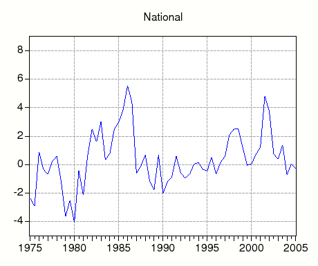
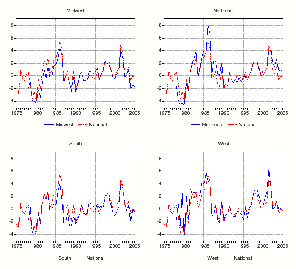
Rent-Price Ratio (Annualized Percent)
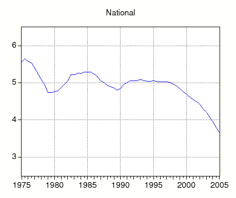
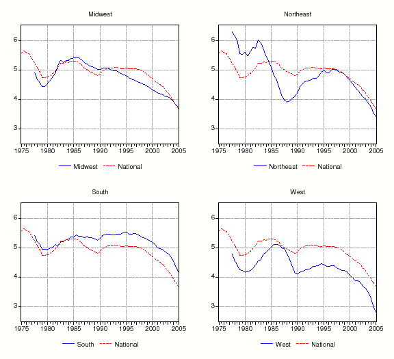
Nominal 10-Year Treasury Inflation Expectations and Real 10-Year Treasury (Annualized Percent)
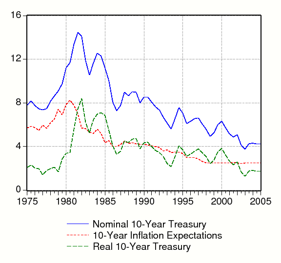
Real 10-Year Treasury and its Future Expected Present Value (Annualized Percent)
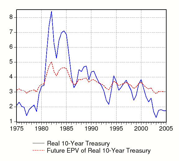
Housing Premia (Annualized Percent)
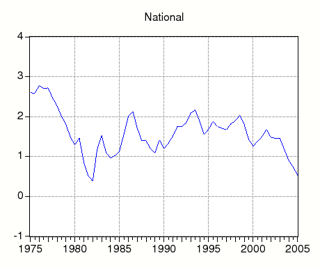
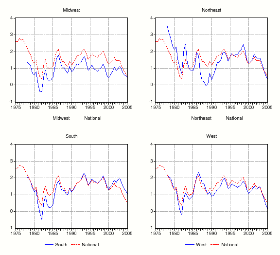
Housing Premia (Annualized Percent), Midwest Cities
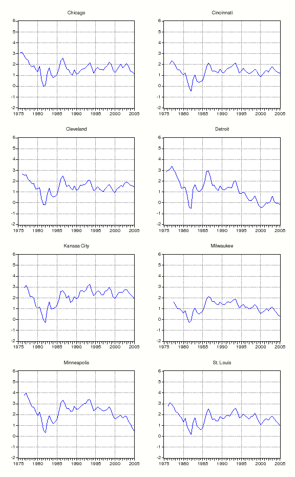
Housing Premia (Annualized Percent), Northeast Cities
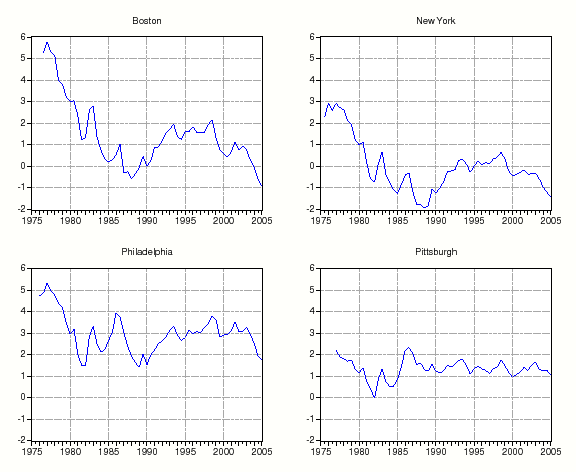
Housing Premia (Annualized Percent), South Cities
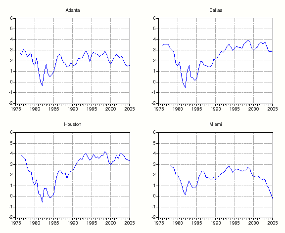
Housing Premia (Annualized Percent), West Cities
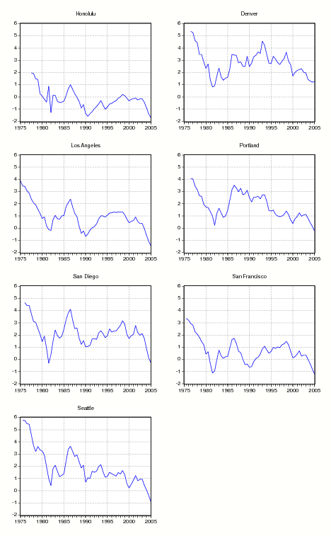
National Log Rent-Price Ratio and its Components
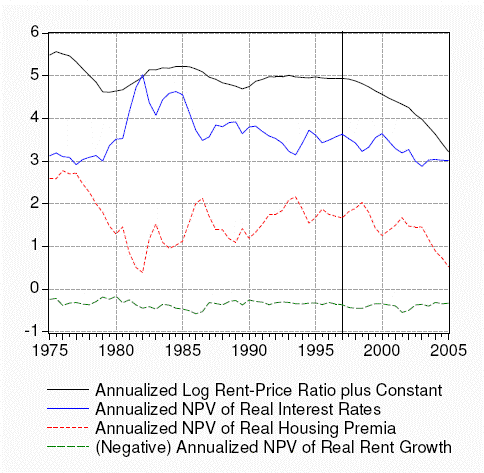
![\begin{eqnarray*} v_{t}-p_{t}=k + \widetilde{i}_{t} +\widetilde{\pi}_{t} -\widetilde{\Delta v}_{t}-(1-\rho)E_{t} \left[\sum_{j=0}^{\infty}\rho^{j}(1-\tau_{t+j+1})\right], \end{eqnarray*}](img36.gif)