Skip to: [Printable Version (PDF)] [Bibliography] [Footnotes]

Finance and Economics Discussion Series: 2006-31 Screen Reader version^♣

Why are Plant Deaths Countercyclical: Reallocation Timing or Fragility?

Andrew Figura ^*

June, 2006

Keywords: Plant deaths, business cycle

Abstract:

Because plant deaths destroy specific capital with large local economic impacts and potentially important macroeconomic effects, understanding the causes of deaths and, in particular, why they are concentrated in cyclical downturns, is important. The reallocation-timing hypothesis posits that plants suffering adverse permanent demand/productivity shocks delay shutdowns until cyclical downturns when plant capacity is less valuable, while the fragility hypothesis posits that shutdowns occur in downturns because the option value of maintaining the plant through weak demand periods is too low. I show that the effect that a plant's specific capital has on the timing of plant deaths differs across these two hypotheses and then use this insight to test the hypotheses' relative importance. I find that fragility is the dominant cause of the countercyclical behavior of plant deaths. This suggests that the endogenous destruction of capital is likely an important amplification and propagation mechanism for cyclical shocks and that stabilization policies have the benefit of reduced capital destruction.

JEL Classification: E20, E22, E32

1. Introduction

This paper investigates and tests theories of the cyclical behavior of plant deaths. Previous research has found that plant deaths (and more generally permanent job destruction) is both sizeable and countercyclical.¹ Because it likely causes the capital specific to a plant (human, physical and organizational) to be destroyed, permanent job destruction is more costly than temporary job destruction, making the understanding of its causes particularly important. The literature has proposed two theories for its countercyclical behavior. The reallocation-timing hypothesis posits that firms do not always react immediately to permanent shocks to plant-level productivity/demand, but instead wait until changes in aggregate demand conditions make permanent changes in plant-level employment more desirable; see, for example, Mortensen and Pissarides (1994), Caballero and Hammour (1996), Davis and Haltiwanger (1990) and Davis (1987). Alternatively, the fragility hypothesis posits that jobs/plants are permanently destroyed in a downturn because the parties to a job/plant lack the incentives to continue their relationship when profitability is temporarily low; see Ramey and Watson (1997).²

Though these two hypotheses have very similar predictions for the cyclical behavior of plant deaths, the causal mechanisms underpinning them are quite different. In particular, the effect that specific capital has on the cyclical behavior of plant deaths differs across these two hypotheses. In a simple model, sunk costs of specific capital cause capacity to be less responsive to changes in demand, which leads the value of capacity to become more cyclically sensitive. This causes firms to concentrate plant deaths in recessions when the opportunity cost (lost capacity) is lower--the reallocation-timing effect. On the other hand, the same model shows that plants with relatively large amounts of specific capital have a larger option value of remaining in business (the sunk cost of their specific capital), and, as a result, predicts that these plants should be less likely to shutdown in response to cyclical shocks--the fragility effect.

Because these two theories cannot be distinguished using aggregate data, I test them using plant-level data. More precisely, I test whether specific capital enhances or mutes the countercyclical response of plant deaths. I find that the data are most supportive of the fragility hypothesis: plant deaths become less countercyclical as the amount of capital is increased. Greater capital insulates plants from cyclical shocks.

The finding that plant fragility is behind the countercyclical movement in plant deaths has some interesting implications for the nature of cyclical fluctuations in economic activity. First, it implies that plant deaths increase endogenously in response to cyclical downturns, with plants containing relatively little specific capital the most vulnerable to shutdowns. Importantly, these shutdowns are not just a shift in the timing of shutdowns, as in reallocation-timing, but are shutdowns that would not have occurred absent a cyclical downturn. Also, estimation results suggest that plants with significant amounts of capital are still vulnerable to cyclical shocks, suggesting that fragility is not limited to a small group of under capitalized plants and thus has potentially important macroeconomic implications. As a consequence of the endogenous increase in plant deaths, the economy's response to adverse cyclical shocks will be amplified by the loss of the jobs and specific capital at fragile plants. In addition, cyclical shocks will be propagated by the introduction of an endogenous supply response to changes in demand-capital is destroyed in recessions and must be rebuilt in expansions. The time and costs associated with the destruction and rebuilding of capital likely extends the effects of shocks well beyond the period in which they occur.³

Several papers have shown that models of reallocation-timing are consistent with aggregate data on job destruction, see Caballero and Hammour (1994, 1996), Mortensen and Pissarides (1994), Davis and Haltiwanger (1990). Others have tested implications of reallocation timing. Davis (1987) shows that reallocation activity (as measured by an employment dispersion index) is negatively correlated with real wages (a proxy for the value of current production), consistent with reallocation-timing. Loungani and Rogerson (1989) show that workers from cyclically sensitive industries are more likely to permanently switch industries in recessions than workers from less cyclically sensitive industries, as a model of reallocation-timing would predict. But neither of these papers considered tests that would distinguish reallocation timing from other theories of countercyclical job destruction, such as fragility. Den Haan, Ramey and Watson (2000) do consider other theories and argue that "pure" reallocation-timing models cannot explain the wage and unemployment experiences of displaced workers, but that models that increase the fragility of jobs by including outside benefits for the parties to a job and/or moral hazard can. This paper differs from den Haan, Ramy, and Watson (2000) by focusing on permanent job destruction, specifically plant deaths, as opposed to the destruction of worker-employer matches. Thus, this paper attempts to understand decisions to destroy all capital specific to a job and plant, not just the capital specific to an employer-worker match.⁴

The next section describes a simple model of permanent job destruction and derives from it a test to distinguish the reallocation timing and fragility hypotheses. The third section describes my data and the construction of the variables that I use in my analysis. The fourth section presents results. The fifth section performs several robustness checks, and the sixth section concludes.

2. The Model

To illustrate the factors that lead plant shutdowns to be concentrated cyclically, I construct a simple model of an economic agent (firm) choosing how many plants to operate and at what utilization rate in response to temporary cyclical and permanent idiosyncratic shocks.⁵ The model shows that plant deaths can become concentrated in recessions for two reasons: first, because relatively large amounts of specific capital increase the cyclical sensitivity of plants' current operating margins, causing plants receiving permanent adverse shocks to delay shutdown until recessions (the reallocation-timing effect); second, because relatively low levels of specific capital reduce the opportunity cost of destroying capacity in response to temporary adverse cyclical shocks (the fragility effect).

Using aggregate data on the cyclical behavior of plant deaths, it is not possible to distinguish which of these two channels is causing the countercyclical behavior of plant deaths. However, the model shows that if the reallocation-timing effect is at work, then increases in specific capital should accentuate the countercyclical behavior of plant deaths, while if fragility is operating, then increases in specific capital should have the opposite effect.

In the model, an economic agent has an investment opportunity to produce a good. To pursue the opportunity, the agent must build a plant, which requires a sunk investment, . measures the amount of capital at a plant that is specific, or that has no alternative use outside the plant.⁶ Also associated with the investment opportunity is a level of permanent demand, , for the output of the plant(s). For ease of exposition, I assume that the possible number of plants the agent can build, , is continuous.

Plant-level technology is constant returns to scale.

$$y_t =u_t n_{t+1}$$ (1)

where is output, is the number of plants, and is the utilization rate, constrained to be between 0 and 1, and I normalize the maximum output of a plant to equal 1. Because all plants are identical, the agent is indifferent about the across-plant distribution of utilization, and one can think of as an average utilization rate.

To produce output, plants incur both variable and fixed costs. Production workers, , are a variable input and are used to increase utilization.

$$u_t =\frac{L_t }{n_{t+1} }$$ (2)

In addition, each plant requires nonproduction workers to maintain it regardless of the current level of utilization. Both types of labor are available at exogenous wage rate . Thus, the fixed cost for each plant is fw.

The firm faces a constant price elasticity of demand (-) for its product.

$$p_t =C_t R_t y_t ^{-\alpha }$$ (3)

where is price. Two types of shocks shift the firm's demand curve: a cyclical shock, , and a shock to its permanent demand, .⁷ oscillates deterministically between low, , and high, , values. Absent a shock, remains the same, but with probability each period, the firm draws a new from the cumulative probability function , which conditional on mean (the current value of is identically distributed.

$$\begin{array}{l} C_t =C^H\,\,if\,\,t=1,3,5,7,\,... \ C_t =C^L\,\,if\,\,t=2,4,6,8,\,... \ \Pr (R_t =R_{t-1} )=(1-\lambda ) \ \Pr (R_t =R)=\lambda \frac{\partial H(R\vert R_{t-1} )}{\partial R}=\lambda h(R\vert R_{t-1} ) \ \end{array}$$ (4)

Each period, the firm chooses the number of plants to operate and the average output per plant to maximize profits subject to the constraint that output can not exceed capacity. The following value function can be used to represent this decision problem.

$$\begin{array}{l} V(n_t ,R_t ,C_t )=Max\left\{ {\begin{array}{l} C_t R_t y_t^{1-\alpha } -wy_t -n_{t+1} fw-F\left( {I_t^C (n_{t+1} -n_t )} \right) \ +\beta EV(n_{t+1} ,R_{t+1} ,C_{t+1} ) \ \end{array}} \right\} \ \,\,\,\,\,\,\,\,\,\,\,\,\,\,\,\,\,\,\,\,\,\,\,\,\,\,\,\,\,\,\,subject\,\,to \ \,\,\,\,\,\,\,\,\,\,\,\,\,\,\,\,\,\,\,\,\,\,\,\,\,\,\,\,\,\,\,0\le y_t \le n_{t+1} \ \end{array}$$ (5)

is an indicator variable equaling 1 if the value in the succeeding parentheses is greater than 0, and is the discount factor for the firm.

Maximizing (5) with respect to and yields the following first order conditions

$$\begin{array}{l} (1-\alpha )R_t C_t y_t^{-\alpha } -w=\mu _t \ \mu _t +\beta E\frac{\partial V}{\partial n_{t+1} }\ge F+fw,\,\,\,\,with\,\,equality\,\,if\,\,n_{t+1} >n_t \ \mu _t -fw+\beta E\frac{\partial V}{\partial n_{t+1} }\le 0,\,\,\,\,with\,\,equality\,\,if\,\,n_{t+1} <n_t \ \mu _t >0,\,\,n_{t+1} -y_t \ge 0,\,\,\mu _t (n_{t+1} -y_t )=0 \ \end{array}$$ (6)

where is the Lagrange multiplier on the constraint that output is less than or equal to capacity. The first equation of (6) shows that the value of relaxing the capacity constraint is the operating margin, defined as the marginal revenue of an additional plant minus marginal variable cost. Utilization will be below 1 if the operating margin at full capacity is negative. The next relationship in (6) shows that new plants are not created until the marginal benefit from plant creation (the current period operating margin plus the discounted expected value of an extra plant) equals the cost: the sunk investment cost and the fixed maintenance cost. The envelope condition shows that

$$\frac{\partial V}{\partial n_t }=\Pr (I_t^C =1)F+\Pr (I_t^C =0)(\mu _t -fw)\le F$$ (7)

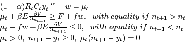
The value of an extra plant is the cost of creating a plant multiplied by the probability that new plants will be created plus the value of having the capacity constraint relaxed minus the fixed cost times the probability that no new plant creation occurs. Given that plants are freely disposed of, the second equation in (6) implies that the marginal value of a plant cannot exceed .

The third relation in (6) describes the decision to shutdown plants. Given that plants are freely disposed of, placing a lower bound of 0 on their value, this relation states that plants are shut down when the operating margin minus the fixed cost turns negative, and the discounted expected future value of the plant is not sufficiently positive to outweigh the current period's negative return.

2.1 Cyclical Concentration of Plant Deaths

The model predicts that the probability of a plant dying is greater in recessions than in expansions. To see this, note that from the third relation in (6), there exists an , , that makes the firm indifferent between shutting down the marginal plant and keeping it open.

$$\mu _t (n_t ,R_D ,C_t )-fw+\beta E\left[ {\left. {\frac{\partial V(n_t ,R_{t+1} ,C_{t+1} )}{\partial n_t }} \right\vert R_D } \right]=0$$ (8)

Next, one can totally differentiate (8) with respect to and

$$\frac{\partial R_D }{\partial C_t }=\frac{-\left( {\frac{\partial \mu _t }{\partial C_t }+\beta E\frac{\partial ^2V}{\partial n_t \partial C_t }} \right)}{\frac{\partial \mu _t }{\partial R_D }+\beta E\frac{\partial ^2V}{\partial n_t \partial R_D }}$$ (9)

To sign this expression, totally differentiate the utilization condition to get

$$\left\{ {\begin{array}{l} \frac{\partial \mu _t }{\partial C_t }=0\,\,\,\,if\,\,y_t <n_t \ \frac{\partial \mu _t }{\partial C_t }>0\,\,\,\,if\,\,y_t =n_t ,\,\,\mu _t -fw+\frac{\beta E\partial V}{\partial n_{t+1} }<F \ \frac{\partial \mu _t }{\partial C_t }=0\,\,\,\,if\,\,\mu _t -fw+\frac{\beta E\partial V}{\partial n_{t+1} }=F \ \end{array}} \right\}$$ (10)

if 0. There exists an analogous relationship for . When utilization is below capacity, operating margins don't change as demand increases; output does instead. When output is at capacity, operating margins increase and output remains constant. Then, when the value of plant creation equals its cost, margins are flat again, as output increases with increases in plant capacity. Using (4) and (7), one gets

$$\frac{\partial V}{\partial n_{t+1} \partial R}>0,\,\,\frac{\partial V}{\partial n_{t+1} \partial C_t }<0,\,\frac{\partial \mu _t }{\partial C_t }-\,\frac{\beta \partial EV}{\partial n_{t+1} \partial C_t }>0$$ (11)

Putting (9)-(11) together, if 0 then at some point between and and

$$R_D^H -R_D^L <0$$ (12)

where superscripts and denote the stage of the cycle. Since the probability of death is the probability that <, this implies that the probability of death for a plant is higher in recessions than in expansions. Intuitively, the marginal value of a plant is positively related to its operating margin, which is procyclical.

2.2 Distinguishing Between Reallocation Timing and Fragility

The probability of a plant dying can be countercyclical for two reasons: reallocation timing or fragility. The two types of permanent job destruction are distinguished by the type of shock that causes them. In reallocation timing, plants are shut down because the permanent level of demand is too low. Thus, shocks to are the fundamental cause of permanent job destruction under reallocation timing. In contrast, fragile plants are shut down because their values are very sensitive to temporary changes in demand. Thus, changes in drive the destruction of fragile plants. Put differently, can be less than for two reasons: first, because is low and, second, because is high. The former case characterizes reallocation timing--the destruction has occurred because has declined since the plant's birth. The latter characterizes fragility--because the cost of scrapping the plant (in terms of lost specific capital) is low, the permanent demand for plant output required to prevent plant closure when operating margins are low, , is high.

Consider first fragility. decreases the fragility of plants by increasing the current and future stream of income from the plant, making it less likely to shut down because of a temporary drop in revenues. To see this, differentiate (8) with respect to and

$$\frac{\partial R_D }{\partial F}=\frac{-\left( {\frac{\partial \mu _t }{\partial F}+\frac{\beta E\partial ^2V}{\partial F\partial n_t }} \right)}{\frac{\partial \mu _t }{\partial R_D }+\frac{\beta E\partial ^2V}{\partial R_D \partial n_t }}$$ (13)

Using (4), (6), (7) and (10), one can show that all four ratios in the numerator and denominator of the expression are positive, which implies that . Intuitively, as increases, the plant must have greater operating margins over its lifetime to recoup its sunk costs, and the value of the plant necessarily increases. As a result, the plant becomes less likely to permanently shutdown solely in response to a change in the cycle from to .⁸

Figure 1 illustrates the insulating effect of plant capital. The lines in the figure show that the value of the marginal plant for firms X and Y increases as demand, CR, increases. Both plants have the same value of . However, plant Y has a higher level of specific capital, and consequently, its value lies everywhere above that of plant . When demand falls by enough to make the value of a plant 0, it is destroyed. For plant , when falls to , its value falls below 0, and it is destroyed. But for the same cyclical change in demand, the value of plant is still positive, and it is not destroyed.

The model only considers the case where the destruction of fragile plants is efficient. More generally, Ramey and Watson (1997) show that if contracting difficulties prevent the producing partners at a plant (financers, entrepreneurs, workers) from behaving opportunistically at the expense of the other partners, the threshold level of specific capital at which plants are fragile may be higher than in an efficient model with perfect information and/or contracts. In terms of the model, this would occur if the continuation value of the plant always had to exceed some level that guaranteed that all partners to a plant were better off maintaining the plant than scrapping it

$$\mu _t -fw+\frac{\beta E\partial V}{\partial n_t }>b$$ (14)

where 0 and is increasing in the scope for opportunistic behavior. Under these conditions, a plant could be scrapped even if its current and discounted expected future value is greater than 0.⁹

There are also plants that shut down because their permanent demand has fallen below a critical threshold. For these plants, changes in affect the timing of the shutdown decision: reallocation timing. Because , these plants are more likely to shut down in recessions than in expansions. And, as shown below, because the difference between and is amplified by increases in specific capital, plants with greater are even more likely to shutdown in recessions. To see this, differentiate (9) with respect to

$$\frac{\partial R_D }{\partial C_t \partial F}=\frac{-\left( ... ...{\beta E\partial ^2V}{\partial n_t \partial R_D }} \right)^2}$$ (15)

Given (4), (6) and (7), and is strictly negative at some points between and . This implies that the negative effect of on becomes even more negative as increases. To understand this result, note that if utilization is procyclical, then from (10) an increase in will increase , but, as shown in (10), this increase only occurs in expansions. As a result, the difference in the value of an extra plant between recessions and expansions increases as increases, and firms receiving a negative permanent demand shock will be more likely to delay plant shutdowns the greater is . Intuitively, as increases, it becomes more costly to adjust capacity in response to cyclical changes in demand, and cyclical changes in demand are reflected instead in changes in the shadow value of the plant, . As the value of the plant become more procyclical, the probability of plant death become more countercyclical.

Figure 2 illustrates this effect. Suppose both plant X and plant Y have experienced declines in permanent demand that would lead to their shutdown when . Because plant Y has more specific capital than plant X, its value is more cyclically sensitive, and as increases from to , plant Y's value increases much more than plant X's. As a result, upon falling to , plant X shutdowns regardless of the stage of the cycle, while, upon falling to , plant Y will only shutdown when .

From the above discussion it is apparent that if fragility is the driving force behind countercyclical plant shutdowns, then plant shutdowns in downturns should be concentrated among plants with little specific capital. On the other hand, if reallocation timing is the driving force, then shutdowns should be concentrated among plants with large amounts of specific capital. Thus, one can test the relative importance of these two effects by seeing whether increases in specific capital cause plant deaths to be more or less countercyclical.

To conduct this test, I use data on permanent plant shutdowns described below. The above analysis suggests the following estimation equation

where if plant dies in period and otherwise, cyc is a measure of the business cycle, includes observable plant characteristics, and is the subset of containing variables that may influence the timing of plant deaths, including measures of a plant's specific capital. Under the reallocation timing hypothesis, the sign of the coefficient on the interaction between cyc and a measure of specific capital should be negative. Under the fragility hypothesis, the coefficient should be positive.

3. Data

I use data from the Census Bureau's Longitudinal Record dataset (LRD), which, in turn, derives from data collected with the Annual Survey of Manufacturers (ASM) and the quinquennial Census of Manufacturers (CM). The CM surveys the universe of about 350,000 manufacturing plants. From the CM a representative sample of between 50,000 to 80,000 plants is chosen to be in the ASM. Plants selected are then surveyed for five consecutive years. Large plants within an industry are selected with certainty, and smaller plants are selected with a probability that varies inversely with plant size. In addition, each year a sample of newly created plants is added to the survey.

To identify deaths, I use methodology similar to Davis, Haltiwanter and Schuh (1996), but add an additional filter to keep only permanent shutdowns (plants that do not reappear in the subsequent year or subsequent CM) in my sample. This method performs well in every ASM panel year except the first, when it is difficult to distinguish true shutdowns from plants that rotate out of the ASM panel. One solution to this problem is to identify certainty plants (which should not be rotated out of the ASM) using employment in the preceding CM and limit the sample in the first year of ASM panels to these plants. However, if, as is likely, the cyclical behavior of deaths for certainty plants is different than non-certainty plants, this could bias results. Instead, I delete the first years of ASM panels from my sample.

As a measure of cyclical conditions, cyc, I use the cyclical component of aggregate manufacturing employment.¹⁰ I also control for the cyclical sensitivity of a plant's industry by including an estimate of the level of cyclical employment in the industry in a given year.¹¹

Turning to variables included in , the model predicts that the amount of specific capital influences the cyclical behavior of plant deaths, though whether it causes deaths to be more or less countercyclical is uncertain. As a measure of the amount of specific capital, I use the book value of equipment and structures. If the value is missing, I use the previous year's value. Using plant physical capital to measure specific capital assumes that a significant portion of capital expenditures are sunk. Previous research, e.g. Ramey and Shapiro (2001), suggests this is the case.¹²

Because all types of capital are likely positively correlated with the complexity of production processes, it is likely that physical capital is positively correlated with the amount of human and organizational capital at a plant. Previous research suggests that much of this capital is also specific.¹³ Thus, the estimated coefficient on the physical capital variable will reflect both the positive correlation between a plant's amount of physical capital and its amount of specific physical capital and the correlation between a plant's physical capital and its specific non-physical capital. Two conditions must be satisfied for plant physical capital to be positively correlated with a plant's total specific capital. First, the portion of a plant's physical capital that is sunk must not be perfectly negatively correlated with a plant's amount of physical capital. If this condition is satisfied, then as a plant's physical capital increases, so does its amount of specific physical capital. Second, a plant's physical capital must not be negatively correlated with its non-physical specific capital. If this condition is satisfied, then a plant's physical capital will be weakly positively correlated with its specific non-physical capital.¹⁴

In some specifications, I also include plant age in .¹⁵ Dunne, Roberts and Samuelson (1989) have shown that the probability of death declines as a plant ages. This could reflect the accumulation of knowledge on how to operate the plant most efficiently, in which case age would also reflect increases in specific capital. Alternatively, the model in section 2 predicts that age responds endogenously to increases in specific capital because plants with more specific capital, , should have a lower probability of dying and should therefore have a higher expected age than plants with less specific capital. Finally, age could reflect the effects of selection, as plants learn about their own productivities, see Jovanovic (1982), and plants with relatively low productivity/demand exit.

To account for other influences on the timing of plant deaths, I also include in whether a plant is part of a multiestablishment firm and the trend growth rate of a plant's four digit industry. As discussed in section 2, market imperfections may cause plants to shut down in periods of low operating margins even if long-term prospects for the plant are bright. If financial market imperfections exist, then a plant's dependence on external sources of financing may be an important determinant of its sensitivity to cyclical shocks. I use a plant's membership in a multi-establishment firm as an indicator of its access to external financing. I use the trend growth rate of a plant's four digit SIC industry to control for differences in the arrival rate of permanent shocks across plants and the interaction between trend growth and the cycle to control for the possibility that these shocks are concentrated in cyclical downturns.¹⁶

Finally, to control for changes in other characteristics of plants across ASM panels, I include ASM panel dummies, e.g. the 1974-1979 panel dummy is equal to one in those years and 0 in other years. As an example of differences across ASM panels, the 1974-79 ASM panel had more plants than the succeeding two panels, the frequency of plant death was greater, and the average size of plant deaths smaller. In some specifications, I also include the interaction between panel dummies and the cycle.

In the model presented in section 2, the sunk capital expenditures of a plant reflect its exogenously given technology. In reality, plant capital may evolve endogenously in response to changes in plant-specific productivity/demand. To the extent this occurs, estimated coefficients will reflect differences in across plants, as well as differences in , and will be biased. One possible solution is to decompose the physical capital of a plant into the total physical capital per worker--the capital intensity of a plant--and the number of workers--the scale of the plant. If productivity differences across plants are Hicks neutral, then they should be reflected in plant scale, but not in capital intensity, which should be determined instead by exogenous technology differences in production methods across different products. Of course, if plants elect to change their technology in response to changes in plant-specific productivity, the distinction between scale and capital intensity becomes less useful.

As a result, my preferred estimation method relies on instrumenting for plant-level physical capital using the average capital for the plant's four digit SIC industry, the average age for the plant's four digit SIC industry, and the average rate of plant turnover. Industry equilibrium models, e.g. Hopenhayn (1992), predict that as sunk costs increase, exit and entry rates (plant turnover) should decline, and average plant age should increase. Thus, these instruments should be relevant. At the same time, a plant's influence on average industry-level capital, age per plant, and average plant turnover should be small enough that the instruments are exogenous to a plant's productivity/demand and reflect only the exogenous capital requirements of the production technologies for the plant's industry. This procedure has the added advantage of controlling for measurement error, which, given the difficulty in providing exact measurements of capital stocks for many ASM reporters and differences between the book value reported by plants and the real value of capital stocks relevant to plants' decisions, is likely large.

I compute an industry's average capital and age per plant using the 1977 Census when plants are classified according to 1972 SIC codes (1975-86) and using the 1987 Census when plants are classified according to 1987 SIC codes (1987-93).¹⁷ In 1989, there is an apparent break in the capital stock data.¹⁸ Hence, in my first stage regression relating plant capital to industry capital, I allow for a break in the intercept and coefficient on industry-level average capital for plants observed in the years 1990-1993. For my measure of plant turnover, I use the sum of the average rate of plant births and the average rate of plant deaths in a four-digit SIC industry minus the absolute value of the difference between these rates. This is akin to measures of excess gross job flows in Davis, Haltiwanger and Schuh (1996). The greater the level of specific capital per plant, the less sensitive to shocks plants should be, and the smaller the amount of plant turnover.

For each year of the ASM, beginning in 1975 and ending in 1993, my sample includes all plants that could have died over the previous year (in effect all plants continuing in operation and all plants that die). I estimate that approximately 54,000 permanent shutdowns occurred over the 1973-1993 period. Because data on plant capital is not available in 1972, my estimation period is shortened to 1975-1993 and includes approximately 46,000 plant deaths.¹⁹

Table 1 compares the characteristics (in the year preceding their death) of the plant deaths in my sample with the universe of manufacturing plants, as represented in the 1977 and 1987 CMs, and with my sample of continuing plants. As shown in panels A and B, plants that shut down are somewhat older and somewhat larger than the average manufacturing plant. The mean size of plant deaths, in terms of employment and capital, is about 50 percent larger, and the average age at death for plants in my sample is one-half year greater than the average age in the manufacturing sector. The distribution of the size for plant deaths is highly skewed, as is the distribution for the universe of plants. Plant deaths in my sample are also much more likely to be part of multiestablishment firms than the average manufacturing plant.

As shown in panel C, the above differences between plants that I observe dying and average plants are driven entirely by differences between plants in the ASM and the universe of plants. Plants selected to be in the ASM are on average older, larger and more likely to be members of multiestablishment firms. Compared to continuing plants in the ASM (compare Panel A to Panel C), my sample of deaths is smaller, younger and less likely to be part of a multiestablishment firm. Thus, while the plants that permanently shut down in a given year in my sample are not inconsequential, in terms of size, and are, in fact, larger than the average manufacturing plant, they are typically smaller than plants in my sample that do not die in a given year.

Figure 3 shows that permanent shutdowns appear to be negatively correlated with economic activity. The top panel shows the estimated number of permanent shutdowns by year (deviated from the mean rate for the relevant ASM panel) along with the cyclical change in aggregate manufacturing employment, as estimated with a band pass filter (the correlation between the two series is -0.44). Shutdowns rise in the recessions of the early 1980s and early 1990s, but change little in other cyclically weak periods, such as 1975 and 1986-87. The bottom panel shows the number of jobs destroyed by these shutdowns.

Before moving to estimation results, it is informative to examine the distribution of capital for plant deaths. In the model presented in section 2, the probability of a plant's death in period depends on the stage of the cycle in and on plant 's specific capital. If reallocation timing is the dominant determinant of the cyclical behavior of plant deaths, then plants with more capital should be relatively more likely to permanently shut down in recessions, and the distribution of the capital size of plant deaths in recessions should be shifted toward high-capital plants relative to the distribution in expansions. If fragility is the dominant explanation, plants with less capital should be relatively more likely to shut down in recessions, and the distribution of the capital size of plant deaths in recessions should be shifted toward low-capital plants relative to the distribution in expansions. Figure 4 shows kernel density plots of the distribution of capital for plant deaths in two different periods: 1982-83 and 1991-1992 and all other years.²⁰ I choose these four years because figure 3 suggests that the negative correlation between plant deaths and cyclical conditions is driven by the events in these years. The x axis is the log difference between the capital size of a plant in the year prior to its death and the average capital size of all ASM plants in that year.²¹ The figure shows that the density at low levels of capital increases much more quickly in the distribution of the early 1980s and 1990s recessions than does the density in the other distribution, suggesting that plants with relatively small amounts of specific capital have a relatively higher probability of dying in recessions than in expansions. The figure offers support for the fragility hypothesis. Of course, it is desirable to control for other characteristics of plant deaths, which I do in the estimation results in the next section.

4. Estimation Results

I estimate (16) using all permanent shutdowns in the LRD from 1975-1993 (as noted above, I am unable to ascertain whether permanent shutdowns occur in the first years of ASM panels and thus exclude those years) and all plants in a given year that continued operating from the previous year. Table 2 shows results from estimating equation (16) as a probit with standard errors computed using White's robust error method. It is interesting to consider, first, the probability of a permanent shutdown conditioning only on the measure of the cycle and panel dummies. The estimation results, shown in column 1) of table 2, are as expected: Deaths are more likely during cyclically weak periods.

Column (2) of the table shows results when the cyclical and secular conditions of a plant's industry, a plant's multiestablishment status, plant physical capital and the interactions between the cycle and physical capital, multiestablishment status and secular conditions are included. The estimated coefficient on capital size is negative and highly significant. This is consistent with the model presented in section 2 and previous research and suggests that capital size reduces the probability of death. In addition, the estimated coefficient on the interaction between capital size and the cycle is significantly positive. The interpretation is that the probability of a plant dying in a downturn increases as levels of physical capital decrease. This suggests that fragility is the dominant determinant of the countercyclical behavior of permanent plant shutdowns.

Multiestablishment status increases the probability of death but insulates plants from cyclical shocks. This is consistent with multiestablishment plants being more likely to receive permanent adverse shocks, but because of their access to outside finance, being less likely to shut down in response to cyclical shocks. Lower trend employment growth in a plant's industry increases the probability of death and also appears to render the timing of plant deaths less countercyclical. Contrary to expectations, increases in the cyclical demand of a plant's industry increases the probability of death.

Column (3) shows results when panel dummies are interacted with the cycle. As shown in figure 3, the negative correlation between the cycle and plant deaths is being driven by the early 1980s and early 1990s recessions, when, as shown in figure 4, small capital size plants were relatively more likely to shut down. Thus it is not surprising that including these interactions absorbs some of the explanatory power of the capital/cycle interaction. Nevertheless, the capital/cycle interaction remains positive and statistically significant.

Columns (4) and (5) shows results when age is added. The probability of plant death is strongly negatively correlated with plant age. The coefficient on the interaction between age and the cycle depends on whether panel dummy/cycle interaction terms are included. When these are excluded, the age interaction is not significant. When they are included, the age interaction is significantly positive, consistent with the fragility hypothesis. In the specification reported in the column (5), the null hypothess that the coefficients on the interactions between the cycle and physical capital and plant age, which should both be correlated with specific capital, are jointly equal to 0 has a p value of 0.0001, consistent with the fragility hypothesis.

As mentioned above, if capital is endogenous and is thereby correlated with plant-specific productivity, or if there exists measurement error in plant capital measures, then the estimates in table 2 are biased. However, instrumental variable estimates will be unbiased. As instruments I use the average capital size, average age and average plant turnover in a plant's four digit SIC industry. Results are reported in table 3.²² Column (1) of table 4 shows that instrumenting for capital increases the estimated coefficient on the interaction between capital size and the cycle several fold, suggesting that measurement error in plant-level capital is a much more important concern than endogenous plant-level capital. A priori, one would expect that removing the influence of plant-level productivity/demand on capital size would cause the coefficient on the interaction between plant capital and the cycle to decrease. The absolute value of the coefficient on capital size increases as well, also consistent with measurement error.²³ Other coefficient estimates are largely as expected. The probability of death is now greater when an industry's cyclical condition is relatively poor (though the estimated coefficient is not statistically significant). When panel dummy/cycle interactions are included, results are little changed, with the exception of the multiestablishment interaction term, which now becomes insignificant.

I also estimated (16) instrumenting for plant-level physical capital and age variables with average industry-level physical capital and including plant turnover as an exogenous right-hand-side variable, rather than instruments. If plant age and average plant-turnover are correlated with types of specific capital other than physical (e.g. organizational or human) capital and the relative importance of these different types of specific capital differs across industries, then this would be appropriate. The null hypothesis that the interactions between the average age of plants, the average physical capital of plants and average plant turnover are jointly equal to 0 has a p value of 0.00001, consistent with the fragility hypothesis. Principal components analysis suggests the existence of only one common component for these three measures, suggesting that the relative importance of different types of specific capital is constant across industries and that the assumption underlying estimates in column (1) are valid.

As demonstrated by Moulton (1990), when variables representing aggregated data are used as right-hand-variables in regressions using micro level independent variables, it is possible that errors are correlated across observations because if observations share an observed characteristic, industry classification in the current application, they are likely to share unobserved characteristics. In this situation, not accounting for the correlation in errors across observations biases standard errors downward. To control for this, columns (3) and (4) allow for correlation in errors within industry groups. As expected, standard errors are larger in this specification, but the coefficient on the interaction between capital size and the cycle remains highly significant.

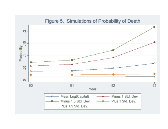
To illustrate the implications of the above results for the countercyclical behavior of plant deaths, figure 5 shows the predicted probability of dying over 1980-1983, using coefficient estimates from column (2) of table 3 and holding all righthandside variables except the aggregate cyclical variable constant at their means. The result is the line with circle symbols. The probability of death rises as the economy enters into recession, reaching a high of nearly 7 percent in 1983. Next, the line with triangle symbols shows the probability of plant death when capital size is reduced by one standard deviation below its mean. Now, the probability of death is significantly more cyclically sensitive, rising to a high of around 15 percent in 1983. The line square symbols shows the probability of plant death at 1.5 standard deviations below the mean. Now the probability of death peaks at over 20 percent. The lines with diamond and plus sign symbols show the probabilities of dying at 1 and 1.5 standard deviations, respectively, above the mean capital size. At these levels of capital size, plant deaths are relatively acyclical.

5. Robustness

I consider the robustness of the estimates presented in section 4 along three dimensions: (1) different parts of the distribution of plant capital (2) different functional forms, and (3) different ASM panels. To see if the finding of fragility is being driven by plants with very large amounts of capital, I exclude plants in the 90^th percentile of the capital size distribution. Columns (1)-(3) of table 4 shows that the estimated coefficient on the interaction between capital size and the cycle is little different from columns (2) and (3) of table 2 and column (2) of table 3, respectively. Next, to see if results are being driven by the smallest plants, in terms of capital size, I exclude those plants in the bottom 20 percent of the capital size distribution. Here, the coefficient on the interaction between capital and the cycle is reduced somewhat, suggesting that fragility is more important at the bottom part of the distribution for capital size. Overall, the results in table 5 suggest that capital intensity decreases fragility across a fairly broad spectrum of the physical capital distribution.

I also repeat the estimation results from table 2 using a logistic regression. Results are little changed. Finally, table 5 shows estimation results from the specifications in columns (2) and (3) of table 2 and column (2) of table 4, respectively, for ASM panels where death rates appear to be relatively insensitive to the cycle--1975-78 and 1985-88--and panels where death rates appear to be quite sensitive--1980-83 and 1990-93. In both sets of years, the estimated coefficient on the interaction between capital size and the cycle is positive when IV is used, but in the 1^st (1975-1978) and 3^rd panels (1985-1988), estimated coefficients are somewhat smaller than in the 2^nd (1980-1983) and 4^th (1990-1993) panels. These results suggest that fragility is a robust phenomenon across different periods of time, but that it was particularly important in post-1980 recessions.

6. Conclusion

Because plant deaths destroy plant and/or industry specific capital, the concentration of plant deaths in recessions has potentially important implications for macroeconomic fluctuations. Reallocation timing posits that plant deaths increase during downturns because cyclical variations in the value of plant capacity cause plants experiencing negative permanent demand or productivity shocks to delay shutdown until a cyclical downturn. Fragility posits that plants lacking sufficient amounts of specific capital are shut down in cyclical downturns because the option value of maintaining them through weak profitability periods is too low. Because both theories predict that plant deaths are countercyclical, aggregate data on plant deaths cannot discriminate between them. However, I show that the two theories have different predictions regarding the effect of specific capital on the cyclical concentration of plant deaths. Reallocation timing predicts that greater specific capital should make plant deaths more countercyclical, while fragility predicts it should make plant deaths less countercyclical. Using this insight, I test the relevance of the two theories and find that fragility is the dominant mechanism behind countercyclical plant deaths.

The existence of fragility implies important amplification and propagation mechanisms for aggregate cyclical shocks. These shocks will be amplified by the destruction of jobs and capital at fragile plants and propagated if building new capital when demand recovers is a time consuming process. If markets are efficient, then fragility implies that only the least valuable plants are shut down in cyclical downturns. However, if financial market imperfections exist, then plant deaths may not necessarily be concentrated among the least valuable plants. Indeed, coefficient estimates imply that plants up to and beyond the mean log capital size are vulnerable to cyclical shocks. In any case, because fragility implies that cyclical shocks cause the destruction of capital that might not otherwise have been destroyed, it may provide an important justification for macroeconomic stabilization policies.

References

Bahk, Byong-Hyong and Michael Gort (1993) "Decomposing Learning by Doing at New Plants," Journal of Political Economy, vol. 101, no. 4, pp. 583.

Baxter, Marianne and Robert G. King, "Measuring Business Cycles: Approximate Band-Pass filters for Economic Time Series," The Review of Economics and Statistics 81, no. 4 (1999): 575-93.

Bernanke, Ben (1993) "Credit in the Macroeconomy," Federal Reserve Bank of New York Quarterly Review, vol. x, no. x, pp. 50-70.

Bernanke Ben and Mark Gertler (1989) "Agency Costs, Net Worth and Business Fluctuations," American Economic Review, vol. 79, no. 1. pp. 14-31.

Bernard, Andrew B. and J. Bradford Jensen (2001) "The Deaths of Manufacturing Plants," NBER working paper no. 9026, July 2002.

Campbell, Jeffrey R. (1998) "Entry, Exit, Embodied Technology, and Business Cycles," Review of Economic Dynamics, Vol. 1, no. 2, pp. 371-407.

Caballero, Ricardo and Mohamad Hammour (1996) "On the Timing and Efficiency of Creative Destruction," Quarterly Journal of Economics, 111(3), 805-852.

Collard-Wexler, Allan "Plant Turnover and Demand Fluctuations in the Ready-Mix Concrete Industry," CES Discussion Paper no. 06-08, March 2006.

Davis, Steven (1987) "Fluctuations in the Pace of Labor Reallocations", Carnegie-Rochester Conference Series on Public Policy 27: 335-402.

Davis, Steven and John Haltiwanger (1990) "Gross Job Creation and Destruction: Microeconomic Evidence and Macroeconomic Implications," NBER Macroeconomics Annual, vol. 5, pp. 123-68.

Davis, Steven, John Haltiwanger, and Scott Schuh (1996) Job Creation and Destruction, Cambridge, MA: MIT Press.

Den Haan, Wouter, Garey Ramey and Joel Watson (2000) "Job Destruction and the Experiences of Displaced Workers," Carnegie-Rochester Conference Series on Public Policy, vol. 52, no. 1, pp. 87-128.

Doms, Mark, Timothy Dunne and Mark J. Roberts (1995) "The Role of Technology Use in the survival and Growth of Manufacturing Plants," International Journal of Industrial Organization, vol. 13, no. 4, pp. 523-542.

Dunne, Timothy and Mark J. Roberts (1991) "Variation in Producer Turnover Across US Manufacturing Industries," in Entry and Market Contestability: An International Comparision, P.A. Geroski and J. Schwalbach Eds., Basil Blackwell.

Dunne, Timothy, Mark F. Roberts and Larry Samuelson (1989) "The Growth and Failure of U.S. Manufacturing Plants," The Quarterly Journal of Economics, vol. 104, no. 4. pp. 671-98.

Figura, Andrew (2006) "Explaining Cyclical Movements in Employment: Creative Destruction or Worker Reallocation," Board of Governors of the Federal Reserve System, mimeo.

Gertler, Mark and Simon Gilchrist (1994) "Monetary Policy, Business Cycles, and the Behavior of Small Manufacturing Firms," The Quarterly Journal of Economics, vol. 109, no. 2, pp. 309-340.

Hopenhayn, Hugo (1992) "Entry, Exit and Firm Dynamics in Long Run Equilibrium," Econometrica, Vol. 60, no. 5, pp. 1127-1150.

Huffman, Gregory W. and Mark A. Wynne (1999) "The Role of Intratemporal Adjustment Costs in a Multisector Economy," Journal of Monetary Economics, Vol. 43, no. 2, pp. 317-350.

Loungani, Prakesh and Richard Rogerson (1989) "Cyclical Fluctuations and the Sectoral Reallocation of Labor: Evidence from the PSID," Journal of Monetary Economics 23, no. 2, pp. 259-273.

Neal, Derek (1995) "Industry-Specific Human Capital: Evidence from Displaced Workers," Journal of Labor Economics, Vol. 13, no. 4, pp. 653-677.

Newey Whitney K. (1987) "Efficient Estimation of Limited Dependent Variable Models with Endogenous Explanatory Variables," Journal of Econometrics, 39, no. 3, pp. 231-250.

Mortensen, Dale and Christopher Pissarides (1994) "Job Creation and Destuction in the Theory of Unemployment, Review of Economic Studies, Vol. 61, no. 208, pp. 849-919.

Phelan, Christopher and Alberto Trejos (2000) "The Aggregate Effects of Sectoral Reallocations," Journal Of Monetary Economics, 45, no. 2, pp. 249-268.

Ramey, Valerie A. and Matthew D. Shapiro (2001) "Displaced Capital: A Study of Aerospace Plant Closings," Journal of Political Economy, 109, no. 5, pp. 958-92.

Ramey, Valerie A. and Matthew D. Shapiro (1998) "Costly Capital Relocation and the Effects of Government Spending," Carnegie-Rochester Conference Series on Public Policy, vol. 48, pp. 145-194.

Rapping, Leonard (1965) "Learning and Workd War II Production Functions," Review of Economics and Statistics, vol.49, no. 4, pp. 568-78.

Ruhm, Christopher (1991) "Are Workers Permanently Scarred by Job Displacements?" American Economic Review, vol. 81, no. 1, pp. 319-23.

Spletzer, James (2000) "The Contribution of Establishment Births and Deaths to Employment Growth," Journal of Business and Economic Statistics, Vol. 18, no. 1, pp. 113-126.

Sutton, John (1990) Sunk Costs and Market Structure, Cambridge, MA: MIT Press.

Syverson, Chad (2004) "Product Substitutability and Productivity Dispersion," Review of Economics and Statistics, vol. 86, no. 2, pp. 534-550.

Topel, Robert (1991) "Specific Capital, Mobility and Wages: Wages Rise with Job Seniority," Journal of Political Economy, vol. 99, no. 1, pp. 145-176.

Townsend, Robert M. (1979) "Optimal Contracts and Competitive Markets with Costly State Verification," Journal of Economic Theory, vol. 21, no. x, pp. 265-93.

 

Table 1. Characteristics of Plant Deaths
Panel A - Plant Deaths (1975-1993)

	Mean	Standard Deviation	Skewness
Capital	2513.3	22159.2	52.03
Employment	78.5	284.9	37.1
Capital Intensity	46.5	308.1	36.7
Age	9.5	8.7	0.9
Multiestablishment	0.573	0.495	-0.296

Table 1. Characteristics of Plant Deaths
Panel B - Census of Manufacturers (1977, 1987)

	Mean	Standard Deviation	Skewness
Capital	1769.4	19648.4	52.8
Employment	52.1	278.8	40.0
Capital Intensity	22.7	76.5	94.0
Age	8.9	7.6	0.8
Multiestablishment	0.223	0.409	0.140

Table 1. Characteristics of Plant Deaths
Panel C - Continuing Plants in the ASM (1975-1993)

	Mean	Standard Deviation	Skewness
Capital	8262.1	48551.9	29.7
Employment	223.8	651.8	17.4
Capital Intensity	42.6	445.1	365.9
Age	13.8	8.4	0.22
Multiestablishment	.71	.45	-0.93

 

Table 2. Estimation Results

	(1)	(2)	(3)	(4)	(5)
Aggregate Cycle	-0.645 (0.013)	-0.922 (0.032)	-0.279 (0.040)	-0.916 (0.034)	-0.331 (0.040)
Panel 2 Interaction			-0.267 (0.031)		-0.316 (0.030)
Panel 3 Interaction			-0.121 (0.071)		-0.124 (0.069)
Panel 4 Interaction			-1.191 (0.037)		-1.149 (0.037)
Industry Cycle		0.030 (0.004)	0.017 (0.004)	0.030 (0.004)	0.019 (0.004)
Industry Trend		-0.099 (0.007)	-0.082 (0.007)	-0.131 (0.006)	-0.114 (0.006)
Capital Size		-0.010 (0.0001)	-0.010 (0.0001)	-0.007 (0.0001)	-0.007 (0.0001)
Age				-0.017 (0.0002)	-0.016 (0.0002)
Multiestablishment		0.002 (0.0004)	0.003 (0.0004)	0.002 (0.0004)	0.003 (0.0004)
Capital Interaction		0.050 (0.005)	0.013 (0.006)	0.048 (0.005)	0.011 (0.006)
Age Interaction				-0.001 (0.011)	0.035 (0.012)
Multiestablishment Interaction		0.241 (0.024)	0.319 (0.026)	0.249 (0.024)	0.307 (0.025)
Industry Trend Interaction		-3.342 (0.338)	-0.474 (0.357)	-3.043 (0.325)	-0.378 (0.344)

Coefficients are marginal effects. Variables are in logs.

 

Table 3. Estimation Results (IV)

	(1)	(2)	(3)	(4)
Aggregate Cycle	-2.327 (0.086)	-1.598 (0.106)	-2.327 (0.242)	-1.598 (0.272)
Panel 2 Interaction		-0.267 (0.037)		-0.267 (0.105)
Panel 3 Interaction		-0.026 (0.083)		-0.026 (0.178)
Panel 4 Interaction		-0.706 (0.040)		-0.706 (0.083)
Industry Cycle	-0.008 (0.004)	-0.014 (0.004)	-0.008 (0.013)	-0.014 (0.014)
Capital Size	-0.013 (0.0003)	-0.013 (0.0004)	-0.013 (0.002)	-0.013 (0.002)
Multiestablishment	0.008 (0.0009)	0.008 (0.0009)	0.008 (0.003)	0.008 (0.003)
Industry Trend Growth	-0.112 (0.007)	-0.102 (0.007)	-0.112 (0.026)	-0.102 (0.026)
Capital Interaction	0.258 (0.015)	0.183 (0.020)	0.258 (0.039)	0.183 (0.046)
Multiestablishment Interaction	-0.031 (0.038)	0.118 (0.049)	-0.031 (0.066)	0.118 (0.083)
Trend Interaction	-1.641 (0.374)	-0.260 (0.386)	-1.641 (0.616)	-0.260 (0.563)

Coefficients are marginal effects. Variables are in logs.

 

Table 4. Excluding plants with large and small amounts of capital

	Excluding top 10 percent of capital size distribution (1)	Excluding top 10 percent of capital size distribution (2)	Excluding top 10 percent of capital size distribution (3)	Excluding bottom 20 percent of capital size distribution (4)	Excluding bottom 20 percent of capital size distribution (5)	Excluding bottom 20 percent of capital size distribution (6)
Aggregate Cycle	-1.006 (0.038)	-0.285 (0.046)	-1.506 (0.190)	-0.827 (0.051)	-0.304 (0.058)	-1.523 (0.135)
2nd Panel Interaction		-0.332 (0.034)	-0.718 (0.043)		0.042 (0.031)	0.005 (0.001)
3rd Panel Interaction		-0.022 (0.082)	-0.475 (0.091)		0.043 (0.065)	0.020 (0.001)
4th Panel Interaction		-1.282 (0.041)	-0.988 (0.044)		-1.202 (0.039)	-0.000 (0.001)
Industry Cycle	0.037 (0.005)	0.024 (0.005)	0.039 (0.005)	0.015 (0.004)	0.000 (0.004)	-0.058 (0.005)
Capital Size	-0.011 (0.0001)	-0.011 (0.0001)	-0.022 (0.0007)	-0.011 (0.0002)	-0.011 (0.0002)	-0.008 (0.0004)
Multiestablishment	0.003 (0.001)	0.004 (0.001)	0.021 (0.001)	0.008 (0.0005)	0.008 (0.0005)	0.003 (0.0008)
Industry Trend Growth	-0.104 (0.008)	-0.804 (0.008)	-0.106 (0.008)	-0.095 (0.007)	-0.082 (0.007)	-0.091 (0.008
Capital Interaction	0.055 (0.006)	0.013 (0.007)	0.228 (0.036)	0.049 (0.007)	0.001 (0.008)	0.127 (0.022)
Multiestablishment Interaction	0.260 (0.026)	0.337 (0.028)	0.103 (0.005)	0.212 (0.024)	0.321 (0.026)	0.245 (0.041)
Trend Interaction	-3.670 (0.378)	-0.522 (0.399)	-0.360 (0.406)	-3.552 (0.335)	-1.183 (0.359)	-0.837 (0.400)

Coefficients are marginal effects. Variables are in logs. Standard errors in columns (3) and (6) reflect correlations in errors within industries.

 

Table 5. Change in Estimated Coefficients over different Periods

	1975-79 & 1985-89 (1)	1975-79 & 1985-89 (2)	1975-79 & 1985-89 (3)	1980-83 & 1990-93 (4)	1980-83 & 1990-93 (5)	1980-83 & 1990-93 (6)
Aggregate Cycle	0.075 (0.055)	0.078 (0.056)	-1.093 (0.257)	-1.476 (0.044)	-0.788 (0.052)	-1.852 (0.0381)
2nd Panel Interaction		-0.088 (0.065)	-0.040 (0.012)		-1.014 (0.037)	-0.465 (0.106)
Industry Cycle	0.046 (0.005)	0.046 (0.005)	-0.040 (0.012)	0.010 (0.006)	-0.006 (0.006)	0.016 (0.023)
Capital Size	-0.011 (0.0001)	-0.011 (0.0001)	-0.011 (0.001)	-0.009 (0.0002)	-0.009 (0.0002)	-0.017 (0.004)
Multiestablishment	0.015 (0.0005)	0.015 (0.0006)	0.013 (0.002)	-0.014 (0.0007)	-0.012 (0.0008)	0.007 (0.006)
Industry Trend Growth	-0.081 (0.009)	-0.081 (0.009)	-0.108 (0.031)	-0.124 (0.010)	-0.099 (0.010)	-0.129 (0.031)
Capital Interaction	-0.006 (0.008)	-0.004 (0.009)	0.0134 (0.028)	0.113 (0.007)	0.046 (0.008)	0.158 (0.059)
Multiestablishment Interaction	-0.133 (0.044)	-0.137 (0.044)	-0.166 (0.101)	0.250 (0.031)	0.457 (0.035)	0.354 (0.112)
Trend Interaction	-2.629 (0.584)	-2.586 (0.587)	-1.740 (1.271)	-1.988 (0.437)	1.393 (0.470)	0.453 (0.984)

Coefficients are marginal effects. Variables are in logs. Standard errors in columns (3) and (6) reflect correlations in errors within industries.

Figure 1. Insulating Effect of Plant Capital

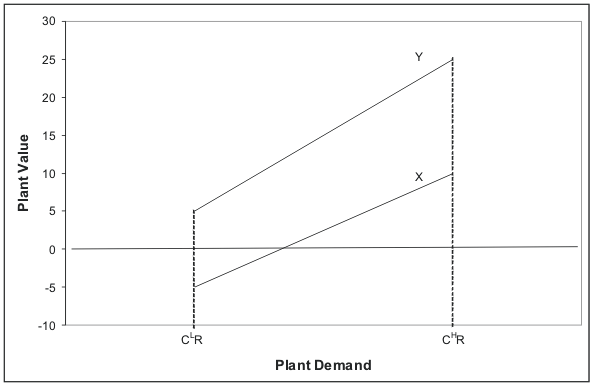
Figure 2. Plant Capital and the Cyclicality of Plant Value

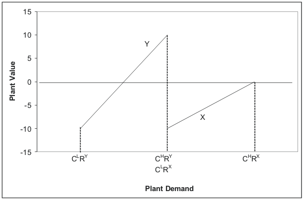
Figure 3. Cyclical Behavior of Deaths.

Figure 4. Distributions of Capital Size for Plant Deaths.

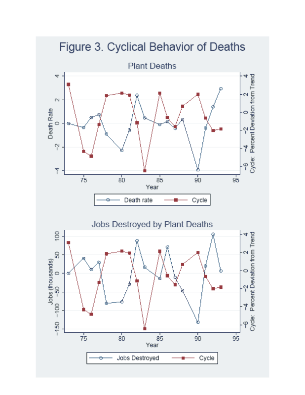
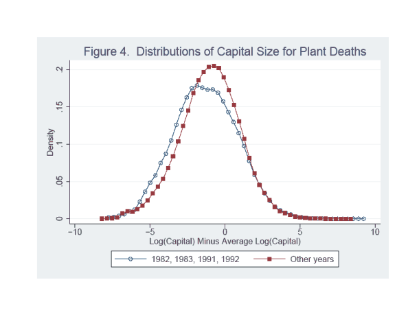
Figure 5. Simulations of Probability of Death.

Footnotes

^*Mail Stop 80, Board of Governors of the Federal Reserve System, Washington DC 20551. Email: [email protected]. The research in this paper was conducted while the author was a Special Sworn Status researcher of the U.S. Census Bureau at the Center for Economic Studies. Research results and conclusions expressed are those of the authors and do not necessarily reflect the views of the Census Bureau or the Federal Reserve Board or its staff. This paper has been screened to insure that no confidential data are revealed. Return to Text

1. See Davis, Haltiwanger, Schuh (1996) and Figura (2006). Return to Text

2. Campbell (1998) proposes that shocks to embodied technology are responsible for the time series behavior of aggregate plant deaths. A weakness of this hypothesis is that it does not explain why plant deaths are strongly positively correlated with cyclical movements in employment at continuing plants. Return to Text

3. Huffman and Wynne (1999), Phelan and Trejos (2000) and Ramey and Shapiro (1998) consider how the costs of moving resources across different sectors can lead to protracted changes in economic activity. Return to Text

4. Another branch of the literature has described the characteristics of plants that permanently shut down, see Dunne, Roberts, and Samuelson (1989) and Bernard and Jensen (2001), but has not investigated how these characteristics vary over the cycle. Davis, Haltiwanger and Schuh (1996) estimate the contribution of births and deaths to cyclical fluctuations in employment in the manufacturing sector, while Spletzer (2000) produces similar estimates for manufacturing and nonmanufacturing plants. But these papers do not investigate why plant deaths are correlated with the cycle. Return to Text

5. Other models, e.g. Mortensen and Pissarides (1994) and Caballero and Hammour (1996), produce cyclical movements in permanent employment changes through cyclical changes in the costs and benefits of production versus job search. Here, a firm balances the costs/benefits of scrapping capacity (plants). Job search is not modeled. Return to Text

6. One can think of the specific capital requirement associated with the product as the outcome of a choice among alternative technologies, each with a different level of specific capital and with the level of unit costs at capacity decreasing with the level of specific capital. I do not model the choice of technology, but posit that the technology menu and permanent demand associated with investment opportunities lead some plants to have relatively large amounts of specific capital and other plants to have relatively small amounts. Return to Text

7. The predictions of the model would be the same if, instead, shocks were to aggregate and idiosyncratic productivities. Return to Text

8. This result can be viewed as extending the analysis of Hopenhayn (1992) and empirical findings of Dunne and Roberts (1991) to cyclical fluctuations. These authors posit and test that industries with low sunk costs should have high average rates of plant births and deaths because they are more sensitive to idiosyncratic shocks. For similar reasons, such plants should also be more sensitive to aggregate cyclical shocks. Return to Text

9. An example of a relationship where opportunistic behavior could lead to inefficient plant deaths is that between a financier and an entrepreneur. In models such as Townsend (1979) and Bernanke and Gertler (1989), information about the returns of a project is asymmetric--only entrepreneurs know the true current period return. Financiers can find out the return, but only at a cost. As a result, the optimal financing arrangement is a contract specifying a fixed payment that does not depend on the current return. If the entrepreneur cannot make the payment, the project is liquidated even if the value remains greater than 0. Thus, asymmetric information in financial relationships is one potentially relevant example of conditions that can cause the scrapping of a plant that, under perfect information, is still valuable. Return to Text

10. I use a bandpass filter, see Baxter and King (1999), to isolate the cyclical component. Return to Text

11. To estimate cyclical employment, I first assemble overlapping 7 year panels of plants continuously in operation over the relevant 7 years. Then I apply a band pass filter to the employment history of each plant to isolate the cyclical component of employment for a plant in the middle year of the 7 year panel. Aggregating across plants in a given industry and dividing by an estimate of the sum of permanent employment for these plants (as estimated using a low pass filter) gives the cyclical component of employment as a percent of total permanent employment for a four digit industry in a given year. Repeating the procedure for the middle year of each ASM panel gives a time series of the cyclical component of employment for each four digit industry. For more details on this approach, see Figura (2006). Return to Text

12. Collard-Wexler (2006) also estimates large sunk costs in the ready-mix concrete industry. Other research also commonly assumes that a portion of physical capital expenditures is sunk, see Syverson (2004) and Sutton (1990). Return to Text

13. Topel (1991), Ruhm (1991) and Neal (1995) argue that some human capital is specific to firms or industries, while Rapping (1965) and Bahk and Gort (1993) describe how organizational capital is largely specific to a particular production process. Return to Text

14. Using plant physical capital as my measure of sunk costs implies that increases in sunk costs also increase capacity. This is consistent with the capacity constraint used in the model presented in section 2 if output is measured in units of maximum output per unit of capacity (in this case, both sides of the capacity constraint are scaled by the same factor). However, such a change in output units necessitates scaling the demand for plant output--equation (3)--by the factor , where is the percent increase in capacity (and maximum output per unit of capacity) caused by an increase in specific capital. As a result, the marginal value of capacity is reduced. This further enhances the negative effect of increases in on the responsiveness of capacity to shocks. Because both the fragility and reallocation timing effects are driven by this effect of increases in , the predictions of the model are preserved when capacity increase with . Return to Text

15. I construct an age variable by noting that if a plant is observed in one CM but not in the previous one, it must have been born between the two CMs. If the plant is included in the ASM between the two CMs, one can use the first observation in the ASM as the date of birth. If not, I assume that the plant's age is the mid-point between the two Census years. Return to Text

16. To construct trend growth rates, I first generate time series of four-digit industry employment using the full ASM for two periods 1973-1986 (for 1972 SIC classification) and 1987-1996 (for 1987 SIC classification) and then fit a linear trend to the log values of these time series. I use the estimated coefficient as my measure of the trend growth rate. Return to Text

17. Capital is unavailable in the 1972 and 1982 Censuses. Return to Text

18. Beginning in 1989, the ASM does not report separate data for machinery and structures, and average levels of capital are considerably below previous levels. Return to Text

19. Because of the filters I have applied to ensure that shutdowns are permanent, my sample includes only a few (56) plants with more than one shutdown. All of these plants have two shutdowns. Return to Text

20. I use the Epanechnikov kernel with a bandwidth of 0.29 for the distribution in years 1982-83 and 1991-92 and a bandwidth of 0.22 in other years. Return to Text

21. I trim the top 1 percent of the distribution before computing this variable. Return to Text

22. The R-squared from the first stage regressions for the level of plant capital and the interaction between plant capital and the cycle are 0.40 and 0.93 respectively Return to Text

23. When the Newey (1987) two-step estimator is used, the null hypothesis of no endogeneity of plant level capital is strongly rejected. Given the sign of the difference in coefficients between the IV and standard methods, this implies that measurement error in plant-level capital stocks is a significant concern. Return to Text

^♣ This version is optimized for use by screen readers. Descriptions for all mathematical expressions are provided in LaTex format. A printable pdf version is available. Return to Text

Home | Economic Research and Data
Accessibility | Contact us
Last update: August 30, 2006