
Bond Risk Premia and Realized
Jump Volatility*
Keywords: Unspanned Stochastic Volatility, Expected Excess Bond Returns, Expectations Hypothesis, Countercyclical Risk Premia, Realized Jump Volatility, Bi-Power Variation
Abstract:
JEL Classification Numbers: G12, G14, E43, C22.
1 Introduction
The Expectations Hypothesis (EH) is well known to be a miserable failure, with bond risk premia being large and time-varying_ A regression of yield changes on yield spreads produces a negative slope coefficient instead of unity, as would be implied by the Expectations Hypothesis (Campbell and Shiller, 1991), and forward rates can predict future excess bond returns (Fama and Bliss, 1987). Indeed Cochrane and Piazzesi (2005) recently showed that using multiple forward rates to predict bond excess returns
generates a very high degree of predictability, with ![]() values of around 30-40 percent. Authors have also used the ARCH in mean (ARCH-M) model to relate excess bond returns to the conditional
volatility of those excess returns including Engle, Lilien, and Robins (1987). They found that both conditional variance and the term structure variables had explanatory power for excess bond returns.
values of around 30-40 percent. Authors have also used the ARCH in mean (ARCH-M) model to relate excess bond returns to the conditional
volatility of those excess returns including Engle, Lilien, and Robins (1987). They found that both conditional variance and the term structure variables had explanatory power for excess bond returns.
The ARCH-M model is a useful tool for considering the relationship between volatility and excess bond returns. But in the last few years, much progress has been made in using high-frequency data to obtain realized volatility estimates. Further, if we observe high-frequency data on the price of an asset, and assume that jumps in the price of this asset are both rare and large, then Barndorff-Nielsen and Shephard (2004), Andersen, Bollerslev, and Diebold (2006), and Huang and Tauchen (2005) show how to detect the days on which jumps occur and how to estimate the magnitude of these jumps. These estimates all have the advantage of being model-free--it has to be assumed that asset prices follow a jump diffusion process, but no specific parametric model needs to be estimated. It then seems natural to try to relate realized volatility and the distribution of jumps to bond risk premia (Tauchen and Zhou, 2006).
Ideally, we would like to study the relationship between risk premia for holding a bond over a given holding period and investors' ex-ante forecasts of volatility and the jump density over that same period. Unfortunately these forecasts are not observed. But, we can easily construct backward-looking rolling estimates of realized volatility, jump intensity, jump mean and jump volatility. Then, treating these as proxies for forecasts of realized volatility, jump intensity, jump mean and jump volatility over the holding period, we can ask whether these risk measures are priced. With this motivation, this paper augments some standard regressions for excess bond returns with measures of realized volatility, jump intensity, jump mean and jump volatility constructed from five-minute S&P500 intraday returns. We also consider using realized jump risk measures constructed from five-minute bond returns, although the theoretical motivation for using the S&P500 returns to construct the jump measure seems strongest, because this is the usual proxy for the market returns of investors.
Our key finding is that augmenting regressions of excess bond returns on forward rates with realized stock market jump volatility greatly increases the predictability of excess bond returns, with ![]() values nearly doubling from 24-29 percent to 48-52 percent (our sample is shorter than that used by Cochrane and Piazzesi (2005) and yields a somewhat smaller
values nearly doubling from 24-29 percent to 48-52 percent (our sample is shorter than that used by Cochrane and Piazzesi (2005) and yields a somewhat smaller ![]() than they obtained). This result is consistent with Tauchen and Zhou (2006), who find that this jump volatility measure can predict the credit spreads better than interest rate factors and volatility factors including option-implied volatility. In
contrast, inclusion of other high-frequency jump measures--jump intensity and jump mean--in the equation for predicting excess bond returns raises the
than they obtained). This result is consistent with Tauchen and Zhou (2006), who find that this jump volatility measure can predict the credit spreads better than interest rate factors and volatility factors including option-implied volatility. In
contrast, inclusion of other high-frequency jump measures--jump intensity and jump mean--in the equation for predicting excess bond returns raises the ![]() by at most a couple of percentage
points. And, if we augment the regression of excess bond returns on forward rates with realized volatility (instead of any of these jump risk measures), the coefficient on realized volatility is significantly positive, but the
by at most a couple of percentage
points. And, if we augment the regression of excess bond returns on forward rates with realized volatility (instead of any of these jump risk measures), the coefficient on realized volatility is significantly positive, but the ![]() goes up only to 35-40 percent.
goes up only to 35-40 percent.
We relate this finding to the recent literature on unspanned stochastic volatility (USV). USV is the hypothesis that bond markets are incomplete and that there is at least one state variable that drives innovations in bond derivatives prices but not innovations in bond yields. As pointed out by Collin-Dufresne and Goldstein (2002), if the bond market is complete, then bond yields can be written as an invertible function of the state variables and so the state variables lie in the span of the term structure of yields. On the other hand, under the USV hypothesis, the state variables do not lie in the span of the term structure of yields. Since expected excess bond returns are a function of the state variables, we argue that this gives a direct test of the USV hypothesis. Similar reasoning is used by Almeida, Graveline, and Joslin (2006) and Joslin (2007). If the USV hypothesis is false, then expected excess bond returns should be spanned by the term structure of yields and so in a regression of excess bond returns on term structure variables and any other predictors, the inclusion of enough term structure control variables should always cause the other predictors to become insignificant. On the other hand, if the USV hypothesis is correct, then the other predictors may be significant as long as they are correlated with the unspanned state variable that does not drive innovations in bond yields but affects the conditional mean of bond yields.
Thus, we interpret our finding that jump volatility is a highly significant predictor of excess bond returns even after controlling for the term structure of forward rates as strong evidence for the USV hypothesis. The USV interpretation is also consistent with the earlier ARCH-M evidence that controlling for the term structure does not eliminate the return-risk trade-off effect on government bond market. Recent work by Ludvigson and Ng (2006) finds that some extracted macroeconomic factors have additional forecasting power for expected bond returns in addition to the information in forward rates and by the same token this is also evidence for the USV hypothesis. Jump volatility however produces a larger improvement in predictive power than these macroeconomic factors and as such represents stronger evidence for USV.
We perform a number of robustness checks, including shortening the holding period, changing the size of the rolling window used to construct the jump measures, using only non-overlapping data, and continue to find an important role for market jump risk in forecasting excess bond returns. The
information content of jump volatility seems to complement that of forward rates, such that the ![]() of the regression on both jump volatility and forward rates is a good bit larger than the
of the regression on both jump volatility and forward rates is a good bit larger than the
![]() from the regression on either variable alone.
from the regression on either variable alone.
Our measure of jump volatility is highly correlated with the price-dividend ratio. We find that in a regression of excess equity returns on jump volatility and the price-dividend ratio, the two predictors are jointly significant but neither is individually significant. In contrast, augmenting our excess bond return forecasting equations with the price-dividend ratio does little to change the significance of jump volatility. In this sense, although both jump volatility and the price-dividend ratio are informative about the cash flow risk, it is the jump volatility that contains more information about discount rate risk.
Standard affine models can explain the violation of the EH only with quite unusual model specifications that may be inconsistent with the second moments of interest rates (Bansal, Tauchen, and Zhou, 2004; Roberds and Whiteman, 1999; Dai and Singleton, 2000). However, much progress has been made recently in constructing models that may explain some of the predictability patterns in excess bond returns. These include models with richer specifications of the market prices of risk or preferences (Dai and Singleton, 2002; Duarte, 2004; Duffee, 2002; Wachter, 2006) and models with regime shifts. For example, Bansal and Zhou (2002), Ang and Bekaert (2002), Evans (2003), and Dai, Singleton, and Yang (2006) use regime-switching models of the term structure to identify the effect of economic expansions and recessions on bond risk premia. Such nonlinear regime-shifts models and the unspanned stochastic volatility hypothesis may be almost observationally equivalent.
The rest of the paper is organized as follows: the next section discusses the jump identification mechanism based on high-frequency intraday data, then Section 3 contains the empirical work on using realized jump volatility to forecast excess bond returns, Section 4 discusses the relationship with the literature on unspanned stochastic volatility in more detail, and Section 5 concludes.
2 Econometric Estimation of Jump Volatility Risk
In this section, we discuss our econometric method for constructing market jump risk measures, which may potentially constitute unspanned volatility factors in predicting excess returns above and beyond those obtained from current yields or forward rates.
Assuming that the stock market price follows a jump-diffusion process (, ), this paper takes a direct approach to identify realized jumps based on the seminal work by Barndorff-Nielsen and Shephard (2006,2004). This approach uses high-frequency data to disentangle realized volatility into separate continuous and jump components (see, Andersen, Bollerslev, and Diebold, 2006; Huang and Tauchen, 2005, as well) and hence to detect days on which jumps occur and to estimate the magnitude of these jumps. The methodology for filtering jumps from bi-power variation is by now fairly standard, but we review it briefly, to keep the paper self-contained.
Let
![]() denote the time
denote the time ![]() logarithmic price of an asset, which evolves in
continuous time as a jump diffusion process:
logarithmic price of an asset, which evolves in
continuous time as a jump diffusion process:
| (1) |
where
| (2) |
where
Barndorff-Nielsen and Shephard (2004) propose two general measures for the quadratic variation process--realized variance and realized bi-power variation--which converge uniformly (as
![]() or
or
![]() ) to different functionals of the underlying jump-diffusion process,
) to different functionals of the underlying jump-diffusion process,
 |
(3) | ||
 |
(4) |
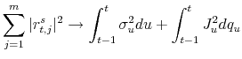
Therefore the difference between the realized variance and bi-power variation is zero when there is no jump and strictly positive when there is a jump (asymptotically). This is the basis of the method for identifying jumps.
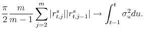
A variety of specific jump detection techniques are proposed and studied by Barndorff-Nielsen and Shephard (2004), Andersen, Bollerslev, and Diebold (2006), and Huang and Tauchen (2005). Here we adopted the ratio
statistics favored by their findings,
 |
(5) |
which converges to a standard normal distribution with appropriate scaling
![\displaystyle ZJ_t \equiv \frac{RJ_t}{\sqrt{[(\frac{\pi}{2})^2+\pi-5] \frac{1}{m}\max(1,% \frac{TP_t}{BV_t^2})}} \overset{d}{\longrightarrow} \mathcal{N} (0, 1)](img25.gif) |
(6) |
This test has excellent size and power properties and is quite accurate in detecting jumps as documented in Monte Carlo work (Huang and Tauchen, 2005).1
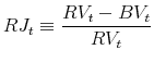
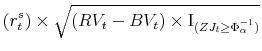
Following Tauchen and Zhou (2006), we further assume that there is at most one jump per day and that the jump size dominates the return when a jump occurs. These assumptions allow us to filter out the daily realized jumps as
 |
(8) |
where
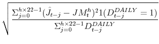
Once the jumps have been identified, we can then estimate the jump intensity, mean and variance as,
 |
|||
with appropriate formulas for the standard error estimates.
These "realized" jump risk measures can greatly facilitate our effort of estimating various risk premia of interest. The reason is that jump parameters are generally very hard to pin down even with both underlying and derivative assets prices, due to the fact that jumps are latent in daily return data and are rare events in financial markets.2. Direct identification of realized jumps and the characterization of time-varying jump risk measures have important implications for interpreting financial market risk premia.
3 Predicting Excess Bond Returns
If jump risk were priced, then the risk premium on any asset over a given holding period should be related to the forecast of the jump density over that holding period. In particular, excess returns on longer term bonds over those on shorter maturity bonds should be related to the forecast of the jump density. The methodology that we described in the previous section allows us to identify and estimate jumps and to construct backward-looking rolling estimates of jump mean, jump intensity and jump volatility. These may in turn be good proxies for the forecasts of future jump mean, jump intensity and jump volatility, and they have the important advantage of being completely model-free--no model has to be specified or estimated to construct them. Accordingly, these rolling jump risk measures may be correlated with risk premia, and may be useful for predicting excess bond returns. Investigating this possibility empirically is the focus of the remainder of this section.
3.1 Variable Definitions and Empirical Strategy
Our measures of realized volatility, jump mean, jump intensity and jump volatility are based on data on the S&P500 index at the five-minute frequency from January 1986 to December 2005, provided by the Institute of Financial Markets. The data cover the period from 9:30am to 4:00pm New York
time each day, for a total of 78 observations per day and can be used to construct continuously compounded returns as the log difference in price index quotes. Using these data and the methods described in the previous section, we constructed the realized volatility at the daily frequency, tested
for jumps on each day, and estimated the magnitude of the jumps on those days when jumps were detected. Let
![]() denote the dummy that is 1 if and only if a jump is detected on day
denote the dummy that is 1 if and only if a jump is detected on day ![]() and recall that
and recall that ![]() denotes the estimated magnitude of the jump on day
denotes the estimated magnitude of the jump on day ![]() . For
our empirical work, let the
. For
our empirical work, let the ![]() -month rolling average realized volatility, jump intensity, jump mean, and jump volatility be defined as, respectively,
-month rolling average realized volatility, jump intensity, jump mean, and jump volatility be defined as, respectively,
 |
|||
 |
|||
 |
|||
 |
where the means and volatilities are calculated only over days where jumps are detected. Realized volatility can be estimated arbitrarily accurately with a fixed span of sufficiently high-frequency data (abstracting from issues of market microstructure noise), whereas this is not true for jump intensity, mean or volatility. For this reason, while we use a relatively short rolling window for estimating realized volatility (
Tauchen and Zhou (2006) use these realized jump risk measures to forecast corporate bond spreads, and find that the realized jump volatility measure can predict these spreads better than interest rate factors and volatility factors including option-implied volatility.
In this paper, we use these realized jump risk measures to forecast excess bond returns. The excess return on holding an ![]() -month bond over the return on holding an
-month bond over the return on holding an ![]() -month bond for a holding period of
-month bond for a holding period of ![]() months is given by
months is given by
![]() where
where ![]() denotes
the annual continuously compounded yield on a
denotes
the annual continuously compounded yield on a ![]() -month zero coupon bond and
-month zero coupon bond and
![]() is the log price of this bond. We used end-of-month data on zero-coupon yields and the three-month risk-free rate from the CRSP Fama-Bliss data, and hence constructed
these excess returns.
is the log price of this bond. We used end-of-month data on zero-coupon yields and the three-month risk-free rate from the CRSP Fama-Bliss data, and hence constructed
these excess returns.
All the regressions for excess bond returns that we consider in this paper are nested within the specification
| (9) |
where
Some summary statistics for these variables are given in Table 1. Realized equity volatility is about 11.5 percentage points (expressed in annualized terms) with a standard deviation of about 5 percentage points. The means of our jump intensity, jump mean and jump volatility measures are 13 percent, 0.06 percentage points and 0.50 percentage points, respectively. Turning to the correlation structure, the excess returns and forward rates are highly collinear. Realized volatility and jump volatility are positively correlated with excess returns. Jump volatility has a strong negative correlation with forward rates (-0.67 to -0.63). The correlation between realized volatility and jump volatility is 0.63, which is not surprising since jump volatility is a component of realized volatility. Now we turn to the main empirical finding in this paper.
3.2 The Main Result
Table 2 shows coefficient estimates, associated t-statistics and ![]() values for several specifications setting
values for several specifications setting ![]() (one-year holding period) and
(one-year holding period) and ![]() (two-year rolling windows in constructing jump risk measures) where the maturity of the longer-term bond
(two-year rolling windows in constructing jump risk measures) where the maturity of the longer-term bond
![]() is set to 24, 36, 48 and 60 months. Forward rates are included in all specifications in this table. The forward rates show the familiar "tent-shaped" pattern, are often individually
significant, and always jointly overwhelmingly significant, with an
is set to 24, 36, 48 and 60 months. Forward rates are included in all specifications in this table. The forward rates show the familiar "tent-shaped" pattern, are often individually
significant, and always jointly overwhelmingly significant, with an ![]() in the range 24-29 percent, which is considerable, although somewhat lower than reported for a different sample period
by Cochrane and Piazzesi (2005). But if we add jump volatility to the regression of excess returns on forward rates, the coefficient on jump volatility is positive and statistically significant for each
in the range 24-29 percent, which is considerable, although somewhat lower than reported for a different sample period
by Cochrane and Piazzesi (2005). But if we add jump volatility to the regression of excess returns on forward rates, the coefficient on jump volatility is positive and statistically significant for each ![]() and the
and the ![]() rises to 48-52 percent. All else equal, higher jump volatility is estimated to lead investors to demand higher future excess returns on
longer-maturity bonds. Adding realized volatility to the regression of excess returns on forward rates also improves the fit notably (Table 2), and the coefficient on realized volatility is statistically significant, which is to be expected since jump volatility is a component of realized
volatility. However, the significance and magnitude of the improvement in
rises to 48-52 percent. All else equal, higher jump volatility is estimated to lead investors to demand higher future excess returns on
longer-maturity bonds. Adding realized volatility to the regression of excess returns on forward rates also improves the fit notably (Table 2), and the coefficient on realized volatility is statistically significant, which is to be expected since jump volatility is a component of realized
volatility. However, the significance and magnitude of the improvement in ![]() is quite a bit weaker. Meanwhile jump mean and jump intensity have no significant predictive power for excess bond
returns. This is true for all choices of the maturity of the longer-term bond,
is quite a bit weaker. Meanwhile jump mean and jump intensity have no significant predictive power for excess bond
returns. This is true for all choices of the maturity of the longer-term bond, ![]() .
.
Table 3 shows the same regressions as Table 2, except omitting the forward rates. If we do not control for the term structure of forward rates, jump volatility remains positively related to future excess returns, but not significantly so. Jump volatility is clearly not the only variable with
predictive power for future excess returns, but it seems to add predictive power over and above the term structure of forward rates that is both statistically and economically significant. And, the information content of jump volatility seems to complement that of forward rates, in that the
![]() of the regression on both jump volatility and forward rates is larger than the
of the regression on both jump volatility and forward rates is larger than the ![]() on either of the variables separately. Controlling for jump volatility does not change the coefficients on the forward rates greatly, suggesting that the term structure of forward rates and jump volatility are measuring different components of bond risk premia. This result is
completely in line with the hypothesis of unspanned stochastic volatility (see Section 4), in that the jump volatility risk factor is not spanned by the current term structure but can forecast bond excess returns above and beyond those achieved by current forward rates.
on either of the variables separately. Controlling for jump volatility does not change the coefficients on the forward rates greatly, suggesting that the term structure of forward rates and jump volatility are measuring different components of bond risk premia. This result is
completely in line with the hypothesis of unspanned stochastic volatility (see Section 4), in that the jump volatility risk factor is not spanned by the current term structure but can forecast bond excess returns above and beyond those achieved by current forward rates.
The ex-post excess returns on holding long term bonds (Figure 2, top panel) averaged around zero during the expansion during the mid and late 1990s, with positive excess returns at some times being offset by negative excess returns as the Federal Open Market Committee (FOMC) was tightening monetary policy during 1994 and around the time of the 1998 Long-Term Capital Management (LTCM) crisis. On the other hand, the excess returns were large and positive during and immediately after the 1990 and 2001 recessions. The predicted excess returns using only the forward rate term structure (middle panel) shows some of this countercyclical variation, but are positive for nearly all of the 1990s and so, on average, overpredict excess returns during these years, while underpredicting excess returns during and immediately after the most recent recession. However, adding the market jump volatility risk measure (bottom panel), the model correctly predicts an average risk premium around zero during most of the 1990s, including negative excess returns in 1994 and 1998, and it is also more successful in predicting high returns during and immediately after the most recent recession. Jump volatility has declined since the last recession, and this may indeed help explain some of the recent decline in longer maturity yields that was referred to by former Federal Reserve Chairman Greenspan as a "conundrum" (discussed further in Kim and Wright, 2005), although jump volatility in 24-month windows ending at the end of our sample is still not especially low by historical standards.
3.3 Robustness Checks
It is well known that severe small-sample size distortions may arise in return prediction regressions with highly persistent regressors and overlapping returns.3 To mitigate this problem, we re-ran our regressions using non-overlapping data. Table 4 shows the results from the same regressions as in Table 2 (i.e. setting ![]() and
and ![]() and various values of
and various values of ![]() ), but using only the forward
rates of each December, so that the holding periods do not overlap. The results are very similar to those in Table 2, and the jump volatility measure is highly significant, though realized volatility is not. The overall predictability increases from 20-26 percent when using only forward rates to
42-45 percent when jump volatility is included.
), but using only the forward
rates of each December, so that the holding periods do not overlap. The results are very similar to those in Table 2, and the jump volatility measure is highly significant, though realized volatility is not. The overall predictability increases from 20-26 percent when using only forward rates to
42-45 percent when jump volatility is included.
Tables 2-4 follow Cochrane and Piazzesi (2005) in considering a one-year holding period (![]() ). But, since we have only 18 non-overlapping periods in our sample,
giving a quite small effective sample size, it also seems appropriate to consider results with a one-quarter holding period (
). But, since we have only 18 non-overlapping periods in our sample,
giving a quite small effective sample size, it also seems appropriate to consider results with a one-quarter holding period (![]() ), for which there are four times as many non-overlapping
periods.4 These results are shown in Table 5. The
), for which there are four times as many non-overlapping
periods.4 These results are shown in Table 5. The ![]() values are lower at this shorter horizon, but jump volatility is again consistently positively and significantly related to future excess bond returns, once we control for the forward rates. Realized volatility is significant at the 5 percent level for two of the four
maturities. The other realized jump measures have no significant association with future excess returns.
values are lower at this shorter horizon, but jump volatility is again consistently positively and significantly related to future excess bond returns, once we control for the forward rates. Realized volatility is significant at the 5 percent level for two of the four
maturities. The other realized jump measures have no significant association with future excess returns.
For the parameter ![]() (rolling window size for jump risk measures), we want to pick a value that is large enough not to give noisy estimates, but small enough to give timely measures of
agents' perceptions of jump risk. A range of reasonable choices might be from 6 to 24 months, and our results are not very sensitive to varying
(rolling window size for jump risk measures), we want to pick a value that is large enough not to give noisy estimates, but small enough to give timely measures of
agents' perceptions of jump risk. A range of reasonable choices might be from 6 to 24 months, and our results are not very sensitive to varying ![]() over this range. For example, Table 6 shows
the results with overlapping data at the one-year horizon (
over this range. For example, Table 6 shows
the results with overlapping data at the one-year horizon (![]() ) and choosing a shorter rolling window for estimating jump statistics
) and choosing a shorter rolling window for estimating jump statistics ![]() . These results are very similar to those in Table 2, in that the total predictability of bond risk premia is nearly doubled with jump volatility included. The slope coefficient for jump volatility remains positive and highly
significant.
. These results are very similar to those in Table 2, in that the total predictability of bond risk premia is nearly doubled with jump volatility included. The slope coefficient for jump volatility remains positive and highly
significant.
3.4 Realized Volatility and Jump Measures Using Bond Data
We also investigated regressing excess returns on the term structure of forward rates and realized volatility and jump measures as in Table 2, except using 30-year Treasury bond futures to construct the realized volatility and jump measures rather than stock price data. We obtained five-minute data on Treasury bond futures from RC Research using the same sample period as before, to make the results comparable.
The results are shown in Table 7. Neither bond realized volatility nor bond jump volatility is statistically significant as a predictor of bond excess returns and the improvement in ![]() from including these variables is very slight. This is consistent with the finding in Andersen and Benzoni (2006) that bond realized volatility is not spanned by the bond yields, although our approach is different in that we are predicting excess bond returns.
from including these variables is very slight. This is consistent with the finding in Andersen and Benzoni (2006) that bond realized volatility is not spanned by the bond yields, although our approach is different in that we are predicting excess bond returns.
The inclusion of bond jump intensity does not help predict bond excess returns either. However, the bond jump mean is significantly negative as a predictor of excess bond returns implying that downward jumps in bond prices are followed by large positive excess returns. Indeed, adding the bond
jump mean to the regression of excess bond returns on forward rates can nearly double the ![]() . This suggests that the bond jump mean may act as an unspanned stochastic mean factor that cannot
be hedged with the current yields but can forecast bond excess returns, which is again consistent with the multi-factor model of incomplete fixed-income market examined by Collin-Dufresne, Goldstein, and Jones (2006a).
. This suggests that the bond jump mean may act as an unspanned stochastic mean factor that cannot
be hedged with the current yields but can forecast bond excess returns, which is again consistent with the multi-factor model of incomplete fixed-income market examined by Collin-Dufresne, Goldstein, and Jones (2006a).
3.5 Forecasting Excess Stock Returns
The empirical link between the equity risk premium and macro-finance state variables has been well established (see, e.g., Campbell and Shiller, 1988b,a; , ; Fama and
French, 1988), but it seems interesting to examine whether the jump variables that help predict excess bond returns might also have some incremental predictive power for excess stock returns. To investigate this, we augmented the usual dividend-yield regression for predicting excess stock
returns with our measures of realized volatility and market jump risk. The three-month excess returns on the stock market are given by
![]() , where
, where ![]() is the return on the S&P500
dividend-inclusive index from the end of month
is the return on the S&P500
dividend-inclusive index from the end of month ![]() to the end of month
to the end of month ![]() and
and
![]() is the three-month risk-free rate from the CRSP Fama-Bliss data at the end of month
is the three-month risk-free rate from the CRSP Fama-Bliss data at the end of month ![]() . The regressions for excess stock returns that we consider are nested within the specification
. The regressions for excess stock returns that we consider are nested within the specification
| (10) |
where
The results are reported in Table 8. Consistent with the existing literature, the price-dividend ratio can predict a small share of return variation (4 percent), and is just statistically significant. On the other hand, none of the high-frequency based risk measures has any detectable predictive
power, except for the jump volatility which on its own gives an ![]() of 7 percent and is statistically significant. Using both the price-dividend ratio and realized jump volatility as
predictors, neither is statistically significant separately (though they are jointly significant), and the
of 7 percent and is statistically significant. Using both the price-dividend ratio and realized jump volatility as
predictors, neither is statistically significant separately (though they are jointly significant), and the ![]() remains at about 7 percent, suggesting that the dividend yield and jump
volatility contain similar information about cash flow risk. Note that the sign of the slope coefficient on the jump volatility variable is negative, meaning that higher jump volatility is associated with lower equity risk premia. This is puzzling, but many papers have found the relationship
between equity risk and return to be unstable and possibly even to have the wrong sign (see, for example Chou, Engle, and Kane, 1992; Bollerslev and Zhou, 2006; Glosten,
Jagannathan, and Runkle, 1993; Campbell, 1987; Turner, Startz,
and Nelson, 1989; Lettau and Ludvigson, 2003; Breen, Glosten, and Jagannathan, 1989, among others). A re-examination of this puzzle may be fruitful along the line of Guo and Whitelaw (2006).
remains at about 7 percent, suggesting that the dividend yield and jump
volatility contain similar information about cash flow risk. Note that the sign of the slope coefficient on the jump volatility variable is negative, meaning that higher jump volatility is associated with lower equity risk premia. This is puzzling, but many papers have found the relationship
between equity risk and return to be unstable and possibly even to have the wrong sign (see, for example Chou, Engle, and Kane, 1992; Bollerslev and Zhou, 2006; Glosten,
Jagannathan, and Runkle, 1993; Campbell, 1987; Turner, Startz,
and Nelson, 1989; Lettau and Ludvigson, 2003; Breen, Glosten, and Jagannathan, 1989, among others). A re-examination of this puzzle may be fruitful along the line of Guo and Whitelaw (2006).
The price-dividend ratio covaries positively with jump volatility (with a correlation coefficient of 0.67), consistent with the finding that adding the price-dividend ratio to a regression of excess stock returns on jump volatility leaves the ![]() about unchanged. This positive correlation can be seen in Figure 3, which shows the time series of both the price-dividend ratio and jump volatility. Both variables appear countercyclical and reflect the aggregate cash flow risk embedded in
stock excess returns. Motivated by this, and the fact that some researchers including Fama and French (1989) have found that the dividend yield helps predict excess bond returns as well as excess stock returns, we investigated augmenting the regressions for excess
bond returns shown in Table 2 with the stock price-dividend ratio. As seen in Table 9, in these regressions the jump volatility remains statistically significant, while the coefficient on the price-dividend ratio is not significantly different from zero. Thus, although
both jump volatility and the price-dividend ratio are informative about the cash flow risk in equity returns, it is the jump volatility that contains more information about the discount rate risk in bond returns.
about unchanged. This positive correlation can be seen in Figure 3, which shows the time series of both the price-dividend ratio and jump volatility. Both variables appear countercyclical and reflect the aggregate cash flow risk embedded in
stock excess returns. Motivated by this, and the fact that some researchers including Fama and French (1989) have found that the dividend yield helps predict excess bond returns as well as excess stock returns, we investigated augmenting the regressions for excess
bond returns shown in Table 2 with the stock price-dividend ratio. As seen in Table 9, in these regressions the jump volatility remains statistically significant, while the coefficient on the price-dividend ratio is not significantly different from zero. Thus, although
both jump volatility and the price-dividend ratio are informative about the cash flow risk in equity returns, it is the jump volatility that contains more information about the discount rate risk in bond returns.
4 Economic Interpretation under Incomplete Markets
In this section, we discuss in more detail the interpretation of regressions of excess bond returns on term structure control variables and other predictors under the incomplete market setting with unspanned stochastic volatility. Under incomplete markets with affine factor dynamics (Collin-Dufresne and Goldstein, 2002), bond yields alone cannot hedge the unspanned volatility risk. However, an important feature of the USV model is that the unspanned risk factor affects the conditional mean and volatility functions of other spanned risk factors (see, Singleton, 2006, pages 322-325). Therefore expected excess bond returns depend not only on the bond yields through the spanned risk factors, but also on the unspanned risk factor. This link provides an explanation for the earlier finding of the ARCH-in-mean effect in bond market (Engle, Lilien, and Robins, 1987), even after controlling for the term structure of yields.
4.1 Unspanned Stochastic Volatility
Recent empirical tests find strong evidence for the existence of unspanned stochastic volatility (see, , ; Casassus, Collin-Dufresne, and Goldstein, 2005; Heidari and Wu, 2003; Collin-Dufresne, Goldstein, and Jones, 2006a; Li and Zhao, 2005; Andersen and Benzoni, 2006, among others).5 The regression of options-implied or estimated volatilities on bond yields is a valid test for the existence of USV, subject to the proper controls for specification error and measurement error in extracting these volatility measures. However, an alternative way is to test the USV implication that the unspanned volatility must predict the bond excess returns above and beyond what can be predicted by the current yields or forward rates.
We illustrate the idea with an ![]() specification (Dai and Singleton, 2000)--which is a three factor affine model with one square-root volatility factor.
Following Collin-Dufresne and Goldstein (2002), all three factor affine models can be rotated such that the state vectors are the spot rate
specification (Dai and Singleton, 2000)--which is a three factor affine model with one square-root volatility factor.
Following Collin-Dufresne and Goldstein (2002), all three factor affine models can be rotated such that the state vectors are the spot rate ![]() , the drift of spot
rate
, the drift of spot
rate
![]() and the variance of spot rate
and the variance of spot rate
![]() . The risk-neutral factor dynamics
. The risk-neutral factor dynamics
![]() is given by
is given by
| (11) |
where
![\begin{displaymath}a^Q=\left[% \begin{array}{c} 0 \\ a_{\mu}^Q \\ a_{V}^Q\end{array}% \right],\ b^Q=\left[% \begin{array}{ccc} 0 & 1 & 0 \\ b_{\mu r}^Q & b_{\mu\mu}^Q & b_{\mu V}^Q \\ 0 & 0 & b_{VV}^Q\end{array}% \right],\ \Omega_0=\left[% \begin{array}{ccc} \underline{V} & \underline{c}_{r\mu} & 0 \\ \underline{c}_{r\mu} & \underline{\sigma}_{\mu} & 0 \\ 0 & 0 & 0\end{array}% \right],\ \Omega_V=\left[% \begin{array}{ccc} 1 & c_{r\mu} & c_{rV} \\ c_{r\mu} & \sigma_{\mu} & c_{\mu V} \\ c_{r V} & c_{\mu V} & \sigma_V \end{array}% \right]\end{displaymath}](img91.gif)
|
The model is maximal, as defined in Dai and Singleton (2000), in that all the parameters are identifiable regardless of the data availability (, ).
Then under complete markets, all trivariate affine models have bond prices of the following form
where
In other words, bond prices do not depend on the unspanned volatility. This condition further restricts the drift and volatility parameter in the
| (14) |
In particular, the restriction
4.2 Predicting Excess Bond Returns
The fact that unspanned stochastic volatility affects the conditional mean of the state vector has important implications for predicting excess bond returns. Letting the market price of risk process be
![]() with
with
![]() , we can transform to the objective dynamics
, we can transform to the objective dynamics
| (15) |
which governs the time-series evolution of the state vector.6 Aside from some special cases, the instantaneous drift under the physical measure
Under incomplete markets, with the bond pricing solution given in eq. (13), the expected excess returns for holding an ![]() -period bond over the returns on holding a
-period bond over the returns on holding a
![]() - period bond for a holding period of
- period bond for a holding period of ![]() periods can be written as
periods can be written as
where the conditional means
and all the terms in eq. (17) are in the span of yields.
Thus, if the bond market is complete, then there should exist no macroeconomic or financial variable that can improve the population forecastability of excess bond returns once we control for the term structure of bond yields. However, if markets are incomplete, then any variable that is correlated with this unspanned volatility factor may add to the predictability of excess bond returns. Of course the challenge is how to find such a proxy for unspanned stochastic volatility. The current methods include implied volatility from fixed-income derivatives markets (e.g., Collin-Dufresne and Goldstein, 2002) and realized volatility from intraday bond prices (Andersen and Benzoni, 2006). Indeed, Almeida, Graveline, and Joslin (2006) and Joslin (2007) find that an unspanned stochastic volatility factor constructed from fixed income options markets is important for predicting bond excess returns. We instead adopt a measure of jump volatility from the equity market, which has an orthogonal innovation relative to the term structure, and find that this also has substantial forecasting power for bond excess returns.
5 Conclusion
There is considerable evidence of predictability in excess returns on a range of assets, but it is especially strong for longer maturity bonds, perhaps because their pricing is not complicated by uncertain cash flows. Part of the predictability may owe to time-variation in the distribution of jump risk, but empirical work on this has been hampered until recently by econometricians' difficulties in identifying jumps. Recently studies (Andersen, Bollerslev, and Diebold, 2006; Tauchen and Zhou, 2006; Huang and Tauchen, 2005; Barndorff-Nielsen and Shephard, 2004) have shown how high-frequency data can be used reliably to detect jumps and to estimate their size, under the assumption that jumps are large and rare, and these methods can then easily be used to construct rolling estimates of jump intensity, jump mean and jump volatility.
A simple implication of jump risk being priced is that these measures should have some predictive power for future excess returns. In this paper, we have found evidence that they do. Augmenting a standard regression of excess bond returns on forward rates with realized jump volatility constructed from high-frequency stock price data, we find that the coefficient on jump volatility is both economically and statistically significant. The predictability of bond risk premia can nearly be doubled by including the jump volatility risk measure. Jump volatility also dominates other risk measures constructed from high-frequency data--namely jump intensity, jump mean, and realized volatility. Although both jump volatility and the price-dividend ratio are informative about the cash flow risk in equity returns, it is the jump volatility that contains more information about the discount rate risk in bond returns.
Jump volatility appears countercyclical--peaking around the 1990 and especially the 2001 recessions. In a number of important episodes, predicted excess returns constructed using both jump volatility and the term structure of forward rates track the actual ex-post excess returns more closely than predicted excess returns constructed using forward rates alone, including during the period in 1994 when the FOMC was tightening monetary policy, the 1998 LTCM crisis, and in the most recent recession. A decline in jump volatility may also account for part of the decline in long-term yields since the FOMC began tightening monetary policy in the middle of 2004. Our result is robust to shortening the holding period, changing the size of the rolling window used to construct the jump measures and using only non-overlapping data. The tent-shape pattern of regression coefficients on the forward term structure however exists regardless whether of whether or not we control for jump volatility.
The existing literature has used implied volatility from fixed-income derivatives (e.g., Collin-Dufresne and Goldstein, 2002) and realized volatility from intraday bond prices (Andersen and Benzoni, 2006) to test the unspanned stochastic volatility hypothesis. Our finding that stock market jump volatility has significant forecasting power for excess bond returns above and beyond that obtained from forward rates alone, is also consistent with this hypothesis.
Journal of Financial Economics, 74, 487-528.
Working Paper.
Standford University GSB.
Working Paper.
Carlson School of Management, University of Minnesota.
Journal of Finance, 57, 1239-1284.
Review of Economics and Statistics.
forthcoming.
Journal of Business and Economic Statistics, 20, 163-182.
Journal of Business and Economic Statistics, 22, 396-409.
Journal of Finance, 57, 1997-2043.
Journal of Financial Econometrics, 2, 1-48.
Journal of Financial Econometrics, 4, 1-30.
Journal of Econometrics, 94, 181-238.
Working Paper.
Columbia University GSB.
Journal of Econometrics, 131, 123-150.
NBER Working Paper No.11841.
Journal of Finance, 44, 1177-1189.
Journal of Financial Economics, 18, 373-399.
Review of Financial Studies, 1, 195-228.
Journal of Finance, 43, 661-676.
Review of Economic Studies, 58, 495-514.
Journal of Financial Economics, 81, 27-60.
Journal of Banking and Finance, 29, 2723-2749.
Journal of Econometrics, 116, 225-258.
Journal of Econometrics, 52, 201-224.
American Economic Review, 95, 138-160.
Journal of Finance, 57, 1685-1730.
Working Paper.
Marshall School of Business, University of Southern California.
Forthcoming.
Journal of Finance, 55, 1943-1978.
Journal of Financial Economics, 63, 415-441.
Review of Financial Studies.
forthcoming.
Review of Financial Studies, 17, 379-404.
Journal of Finance, 57, 405-443.
Mathematical Finance, 6, 379-406.
Econometrica, 55, 391-407.
Journal of Finance, 53, 1269-1300.
Economic Journal, 113, 345-389.
American Economic Review, 77, 680-692.
Journal of Financial Economics, 22, 3-25.
Journal of Financial Economics, 25, 23-49.
Journal of Finance, 58, 2219-2248.
Journal of Finance, 1393-1414.
Journal of Finance, 48, 1779-1801.
Journal of Finance, 61, 1433-1463.
Journal of Fixed Income, 13, 75-86.
Review of Financial Studies, 6, 327-343.
Journal of Financial Econometrics, 3, 456-499.
Working Paper.
Standford University GSB.
Finance and Economics Discussion Series.
Federal Reserve Board.
Elsevier Science B.V., Amsterdam.
Forthcoming.
Journal of Finance.
Working Paper.
Department of Economics, New York University.
Journal of Financial Economics, 3, 125-144.
Journal of Financial Economics, 63, 3-50.
Journal of Monetary Economics, 44, 555-580.
Princeton University Press.
Journal of Financial Economics, 54, 375-421.
Working Paper.
Federal Reserve Board.
Working Paper.
Harvard University.
Journal of Financial Economics, 25, 3-22.
Journal of Financial Economics, 68, 201-232.
Journal of Financial Economics, 79, 365-399.
| Summary statistics | |||||||||||
|---|---|---|---|---|---|---|---|---|---|---|---|
| Mean | 0.91 | 1.63 | 2.23 | 2.5 | 4.94 | 6.09 | 6.44 | 11.57 | 0.13 | 0.06 | 0.5 |
| Std. Dev. | 1.42 | 2.7 | 3.74 | 4.58 | 2.1 | 1.62 | 1.42 | 5.26 | 0.06 | 0.07 | 0.23 |
| Skewness | -0.09 | -0.16 | -0.19 | -0.25 | -0.16 | -0.18 | 0.18 | 1.27 | 0.37 | 0.2 | 0.87 |
| Kurtosis | 2.17 | 2.36 | 2.46 | 2.58 | 2.33 | 2.43 | 1.92 | 4.69 | 1.79 | 3.09 | 2.2 |
Notes: This table summarizes the main variables used in the empirical exercise. The variable definitions are the same as given in Section 3.1:
![]() are the excess returns on holding an
are the excess returns on holding an ![]() -month bond over the return
on holding an
-month bond over the return
on holding an ![]() -month bond for a holding period of
-month bond for a holding period of ![]() months;
months; ![]() denotes the one-year forward rate ending
denotes the one-year forward rate ending ![]() months; and
months; and
![]() ,
,
![]() ,
,
![]() and
and
![]() denote the realized volatility and jump measures in rolling windows ending on the last day of month
denote the realized volatility and jump measures in rolling windows ending on the last day of month ![]() .
.
| Correlation matrix | |||||||||||
|---|---|---|---|---|---|---|---|---|---|---|---|
| R1 | 1 | 0.98 | 0.96 | 0.92 | 0.22 | 0.35 | 0.33 | 0.12 | 0.11 | -0.1 | 0.16 |
| R2 | 1 | 0.99 | 0.97 | 0.17 | 0.32 | 0.31 | 0.14 | 0.08 | -0.13 | 0.2 | |
| R3 | 1 | 0.99 | 0.13 | 0.31 | 0.32 | 0.1 | 0.1 | -0.17 | 0.19 | ||
| R4 | 1 | 0.1 | 0.29 | 0.32 | 0.08 | 0.09 | -0.2 | 0.2 | |||
| R5 | 1 | 0.91 | 0.78 | -0.27 | 0.09 | 0.41 | -0.65 | ||||
| R6 | 1 | 0.94 | -0.41 | 0.27 | 0.19 | -0.67 | |||||
| R7 | 1 | -0.48 | 0.44 | -0.02 | -0.63 | ||||||
| R8 | 1 | -0.37 | 0.29 | 0.63 | |||||||
| R9 | 1 | -0.44 | -0.27 | ||||||||
| R10 | 1 | -0.26 | |||||||||
| R11 | 1 |
Notes: This table summarizes the main variables used in the empirical exercise. The variable definitions are the same as given in Section 3.1:
![]() are the excess returns on holding an
are the excess returns on holding an ![]() -month bond over the return
on holding an
-month bond over the return
on holding an ![]() -month bond for a holding period of
-month bond for a holding period of ![]() months;
months; ![]() denotes the one-year forward rate ending
denotes the one-year forward rate ending ![]() months; and
months; and
![]() ,
,
![]() ,
,
![]() and
and
![]() denote the realized volatility and jump measures in rolling windows ending on the last day of month
denote the realized volatility and jump measures in rolling windows ending on the last day of month ![]() .
.
| Intercept | t-statistic |
t-statistic |
t-statistic |
t-statistic |
t-statistic |
t-statistic |
t-statistic |
t-statistic |
||||||||
|---|---|---|---|---|---|---|---|---|---|---|---|---|---|---|---|---|
| -1.37 | (-1.00) | -0.73 | (-2.89) | 1.91 | -3.7 | -0.89 | (-1.74) | 0.24 | ||||||||
| -3.97 | (-2.81) | -0.81 | (-4.15) | 1.95 | -5.04 | -0.65 | (-1.53) | 1.68 | (-3.19) | 0.35 | ||||||
| -1.36 | (-1.00) | -0.73 | (-2.88) | 1.93 | -3.46 | -0.93 | (-1.61) | 0.52 | (-0.1) | 0.24 | ||||||
| -0.84 | (-0.59) | -0.64 | (-2.29) | 1.99 | -3.92 | -1.09 | (-2.09) | -3.47 | (-0.84) | 0.25 | ||||||
| -5.82 | (-3.80) | -0.58 | (-2.89) | 2.02 | -5.67 | -0.75 | (-1.83) | 4.25 | (-4.75) | 0.48 |
Notes: This table reports the coefficient estimates in a regression of the excess returns on a ![]() -month bond over those on a 12 month bond, with a holding period of
12 months, on the term structure of forward rates, a one-month rolling window of realized S&P500 volatility and a 24 month rolling window of S&P500 jump mean, jump intensity, and jump volatility, constructed as described in the text. Observations are at the monthly frequency (end-of-month).
T-statistics are shown in parentheses and are based on Newey-West standard errors with a lag truncation parameter of 11.
-month bond over those on a 12 month bond, with a holding period of
12 months, on the term structure of forward rates, a one-month rolling window of realized S&P500 volatility and a 24 month rolling window of S&P500 jump mean, jump intensity, and jump volatility, constructed as described in the text. Observations are at the monthly frequency (end-of-month).
T-statistics are shown in parentheses and are based on Newey-West standard errors with a lag truncation parameter of 11.
| Intercept | t-statistic |
t-statistic |
t-statistic |
t-statistic |
t-statistic |
t-statistic |
t-statistic |
t-statistic |
||||||||
|---|---|---|---|---|---|---|---|---|---|---|---|---|---|---|---|---|
| -2.78 | (-1.16) | -1.6 | (-3.19) | 3.89 | -3.71 | -1.77 | (-1.81) | 0.25 | ||||||||
| -7.98 | (-3.19) | -1.76 | (-4.61) | 3.97 | -5.02 | -1.29 | (-1.65) | 3.36 | (-3.37) | 0.38 | ||||||
| -2.83 | (-1.19) | -1.6 | (-3.27) | 3.81 | -3.45 | -1.63 | (-1.49) | -2 | (-0.22) | 0.26 | ||||||
| -1.87 | (-0.77) | -1.44 | (-2.66) | 4.03 | -3.83 | -2.1 | (-2.06) | -5.96 | (-0.78) | 0.27 | ||||||
| -11.6 | (-4.08) | -1.31 | (-3.74) | 4.11 | -6.18 | -1.48 | (-1.99) | 8.42 | (-4.92) | 0.52 |
Notes: This table reports the coefficient estimates in a regression of the excess returns on a ![]() -month bond over those on a 12 month bond, with a holding period of
12 months, on the term structure of forward rates, a one-month rolling window of realized S&P500 volatility and a 24 month rolling window of S&P500 jump mean, jump intensity, and jump volatility, constructed as described in the text. Observations are at the monthly frequency (end-of-month).
T-statistics are shown in parentheses and are based on Newey-West standard errors with a lag truncation parameter of 11.
-month bond over those on a 12 month bond, with a holding period of
12 months, on the term structure of forward rates, a one-month rolling window of realized S&P500 volatility and a 24 month rolling window of S&P500 jump mean, jump intensity, and jump volatility, constructed as described in the text. Observations are at the monthly frequency (end-of-month).
T-statistics are shown in parentheses and are based on Newey-West standard errors with a lag truncation parameter of 11.
| Intercept | t-statistic |
t-statistic |
t-statistic |
t-statistic |
t-statistic |
t-statistic |
t-statistic |
t-statistic |
||||||||
|---|---|---|---|---|---|---|---|---|---|---|---|---|---|---|---|---|
| -4.6 | (-1.53) | -2.43 | (-3.71) | 5.41 | -3.88 | -2.19 | (-1.70) | 0.29 | ||||||||
| -11.33 | (-3.39) | -2.63 | (-5.26) | 5.51 | -5.12 | -1.58 | (-1.52) | 4.34 | (-3.06) | 0.4 | ||||||
| -4.7 | (-1.57) | -2.44 | (-3.85) | 5.23 | -3.57 | -1.92 | (-1.30) | -4.04 | (-0.35) | 0.29 | ||||||
| -3.4 | (-1.13) | -2.22 | (-3.13) | 5.59 | -3.94 | -2.63 | (-1.90) | -7.87 | (-0.76) | 0.3 | ||||||
| -16.11 | (-4.06) | -2.05 | (-4.46) | 5.69 | -6.08 | -1.82 | (-1.79) | 10.99 | (-4.41) | 0.52 |
Notes: This table reports the coefficient estimates in a regression of the excess returns on a ![]() -month bond over those on a 12 month bond, with a holding period of
12 months, on the term structure of forward rates, a one-month rolling window of realized S&P500 volatility and a 24 month rolling window of S&P500 jump mean, jump intensity, and jump volatility, constructed as described in the text. Observations are at the monthly frequency (end-of-month).
T-statistics are shown in parentheses and are based on Newey-West standard errors with a lag truncation parameter of 11.
-month bond over those on a 12 month bond, with a holding period of
12 months, on the term structure of forward rates, a one-month rolling window of realized S&P500 volatility and a 24 month rolling window of S&P500 jump mean, jump intensity, and jump volatility, constructed as described in the text. Observations are at the monthly frequency (end-of-month).
T-statistics are shown in parentheses and are based on Newey-West standard errors with a lag truncation parameter of 11.
| Intercept | t-statistic |
t-statistic |
t-statistic |
t-statistic |
t-statistic |
t-statistic |
t-statistic |
t-statistic |
||||||||
|---|---|---|---|---|---|---|---|---|---|---|---|---|---|---|---|---|
| -6.2 | (-1.79) | -2.96 | (-3.71) | 6.1 | -3.56 | -2.14 | (-1.38) | 0.28 | ||||||||
| -14 | (-3.52) | -3.2 | (-5.20) | 6.22 | -4.55 | -1.43 | (-1.15) | 5.03 | (-2.77) | 0.38 | ||||||
| -6.45 | (-1.86) | -2.98 | (-4.01) | 5.65 | -3.18 | -1.45 | (-0.80) | -10.2 | (-0.74) | 0.29 | ||||||
| -4.84 | (-1.46) | -2.73 | (-3.19) | 6.31 | -3.58 | -2.64 | (-1.56) | -8.93 | (-0.71) | 0.29 | ||||||
| -19.98 | (-4.06) | -2.51 | (-4.62) | 6.43 | -5.51 | -1.7 | (-1.37) | 13.16 | (-4.07) | 0.51 |
Notes: This table reports the coefficient estimates in a regression of the excess returns on a ![]() -month bond over those on a 12 month bond, with a holding period of
12 months, on the term structure of forward rates, a one-month rolling window of realized S&P500 volatility and a 24 month rolling window of S&P500 jump mean, jump intensity, and jump volatility, constructed as described in the text. Observations are at the monthly frequency (end-of-month).
T-statistics are shown in parentheses and are based on Newey-West standard errors with a lag truncation parameter of 11.
-month bond over those on a 12 month bond, with a holding period of
12 months, on the term structure of forward rates, a one-month rolling window of realized S&P500 volatility and a 24 month rolling window of S&P500 jump mean, jump intensity, and jump volatility, constructed as described in the text. Observations are at the monthly frequency (end-of-month).
T-statistics are shown in parentheses and are based on Newey-West standard errors with a lag truncation parameter of 11.
| Intercept | t-statistic |
t-statistic |
t-statistic |
t-statistic |
t-statistic |
|||||
|---|---|---|---|---|---|---|---|---|---|---|
| 0.52 | -0.91 | 0.53 | -0.77 | 0.02 | ||||||
| 0.56 | -0.74 | 2.62 | -0.5 | 0.01 | ||||||
| 1.04 | -2.37 | -2.08 | (-0.45) | 0.01 | ||||||
| 0.4 | -0.66 | 1 | -0.9 | 0.03 |
Notes: As for Table 2, except that the predictors are realized volatility and jump risk measures without controlling for forward rates.
| Intercept | t-statistic |
t-statistic |
t-statistic |
t-statistic |
t-statistic |
|||||
|---|---|---|---|---|---|---|---|---|---|---|
| 0.81 | -0.74 | 1.12 | -0.85 | 0.02 | ||||||
| 1.14 | -0.84 | 3.65 | -0.39 | 0.01 | ||||||
| 1.94 | -2.47 | -5.05 | (-0.60) | 0.02 | ||||||
| 0.42 | -0.36 | 2.4 | -1.14 | 0.04 |
Notes: As for Table 2, except that the predictors are realized volatility and jump risk measures without controlling for forward rates.
| Intercept | t-statistic |
t-statistic |
t-statistic |
t-statistic |
t-statistic |
|||||
|---|---|---|---|---|---|---|---|---|---|---|
| 1.41 | -0.91 | 1.12 | -0.61 | 0.01 | ||||||
| 1.35 | -0.77 | 6.53 | -0.54 | 0.01 | ||||||
| -2.82 | -2.67 | -9.45 | (-0.85) | 0.03 | ||||||
| 0.65 | -0.41 | 3.13 | -1.13 | 0.04 |
Notes: As for Table 2, except that the predictors are realized volatility and jump risk measures without controlling for forward rates.
| Intercept | t-statistic |
t-statistic |
t-statistic |
t-statistic |
t-statistic |
|||||
|---|---|---|---|---|---|---|---|---|---|---|
| 1.71 | -0.91 | 1.08 | -0.47 | 0.01 | ||||||
| 1.6 | -0.77 | 6.76 | -0.48 | 0.01 | ||||||
| 3.36 | -2.85 | -13.56 | (-1.04) | 0.04 | ||||||
| 0.5 | -0.26 | 3.98 | -1.24 | 0.04 |
Notes: As for Table 2, except that the predictors are realized volatility and jump risk measures without controlling for forward rates.
| Intercept | t-statistic |
t-statistic |
t-statistic |
t-statistic |
t-statistic |
t-statistic |
t-statistic |
t-statistic |
||||||||
|---|---|---|---|---|---|---|---|---|---|---|---|---|---|---|---|---|
| -1.79 | (-1.03) | -0.65 | (-2.29) | 1.54 | -1.99 | -0.55 | (-0.79) | 0.2 | ||||||||
| -3.23 | (-0.96) | -0.72 | (-2.72) | 1.57 | -2.3 | -0.42 | (-0.62) | 1.14 | -0.6 | 0.24 | ||||||
| -1.79 | (-1.00) | -0.65 | (-2.13) | 1.54 | -2.01 | -0.54 | (-0.68) | -0.28 | (-0.04) | 0.2 | ||||||
| -1.61 | (-0.73) | -0.61 | (-1.75) | 1.53 | -2.04 | -0.58 | (-0.72) | -0.78 | (-0.10) | 0.2 | ||||||
| -5.84 | (-2.73) | -0.41 | (-2.36) | 1.52 | -2.93 | -0.39 | (-0.67) | 4.23 | -3.09 | 0.42 |
Notes: As for Table 2, except that only end-of-year observations are used to avoid overlapping holding periods. Standard errors are heteroskedasticity-robust, but make no correction for serial correlation.
| Intercept | t-statistic |
t-statistic |
t-statistic |
t-statistic |
t-statistic |
t-statistic |
t-statistic |
t-statistic |
||||||||
|---|---|---|---|---|---|---|---|---|---|---|---|---|---|---|---|---|
| -4.19 | (-1.28) | -1.46 | (-2.43) | 3.17 | -1.92 | -0.98 | (-0.69) | 0.23 | ||||||||
| -6.88 | (-1.06) | -1.59 | (-2.81) | 3.21 | -2.18 | -0.75 | (-0.53) | 2.11 | -0.57 | 0.26 | ||||||
| -4.29 | (-1.26) | -1.52 | (-2.52) | 3.16 | -2.05 | -0.83 | (-0.53) | -4.2 | (-0.29) | 0.24 | ||||||
| -3.59 | (-0.85) | -1.34 | (-1.91) | 3.12 | -1.97 | -1.09 | (-0.65) | -2.7 | (-0.18) | 0.23 | ||||||
| -12.23 | (-2.78) | -0.99 | (-2.99) | 3.11 | -3.02 | -0.67 | (-0.58) | 8.39 | -3.07 | 0.45 |
Notes: As for Table 2, except that only end-of-year observations are used to avoid overlapping holding periods. Standard errors are heteroskedasticity-robust, but make no correction for serial correlation.
| Intercept | t-statistic |
t-statistic |
t-statistic |
t-statistic |
t-statistic |
t-statistic |
t-statistic |
t-statistic |
||||||||
|---|---|---|---|---|---|---|---|---|---|---|---|---|---|---|---|---|
| -6.52 | (-1.47) | -2.16 | (-2.65) | 4.37 | -1.89 | -1.13 | (-0.56) | 0.26 | ||||||||
| -9.83 | (-1.12) | -2.34 | (-2.96) | 4.41 | -2.11 | -0.83 | (-0.42) | 2.61 | -0.52 | 0.29 | ||||||
| -6.69 | (-1.45) | -2.28 | (-2.81) | 4.36 | -2.05 | -0.86 | (-0.39) | -7.21 | (-0.37) | 0.26 | ||||||
| -5.51 | (-0.97) | -1.98 | (-2.05) | 4.29 | -1.94 | -1.31 | (-0.56) | -4.51 | (-0.22) | 0.26 | ||||||
| -17.13 | (-2.66) | -1.56 | (-3.54) | 4.29 | -2.94 | -0.72 | (-0.43) | 11.07 | -2.74 | 0.45 |
Notes: As for Table 2, except that only end-of-year observations are used to avoid overlapping holding periods. Standard errors are heteroskedasticity-robust, but make no correction for serial correlation.
| Intercept | t-statistic |
t-statistic |
t-statistic |
t-statistic |
t-statistic |
t-statistic |
t-statistic |
t-statistic |
||||||||
|---|---|---|---|---|---|---|---|---|---|---|---|---|---|---|---|---|
| -8.77 | (-1.63) | -2.51 | (-2.40) | 4.34 | -1.48 | -0.44 | (-0.17) | 0.25 | ||||||||
| -12.16 | (-1.12) | -2.68 | (-2.62) | 4.39 | -1.6 | -0.14 | (-0.05) | 2.67 | -0.43 | 0.27 | ||||||
| -9.09 | (-1.61) | -2.72 | (-2.77) | 4.33 | -1.66 | 0.05 | (-0.02) | -13.29 | (-0.55) | 0.26 | ||||||
| -7.89 | (-1.13) | -2.34 | (-1.97) | 4.27 | -1.52 | -0.6 | (-0.20) | -3.93 | (-0.16) | 0.25 | ||||||
| -21.21 | (-2.55) | -1.79 | (-2.99) | 4.25 | -2.21 | 0.03 | (-0.01) | 12.98 | -2.44 | 0.42 |
Notes: As for Table 2, except that only end-of-year observations are used to avoid overlapping holding periods. Standard errors are heteroskedasticity-robust, but make no correction for serial correlation.
| Intercept | t-statistic |
t-statistic |
t-statistic |
t-statistic |
t-statistic |
t-statistic |
t-statistic |
t-statistic |
||||||||
|---|---|---|---|---|---|---|---|---|---|---|---|---|---|---|---|---|
| -0.62 | (-1.34) | -0.42 | (-2.48) | 1.19 | -3.16 | -0.66 | (-2.43) | 0.12 | ||||||||
| -1.37 | (-2.65) | -0.44 | (-2.58) | 1.19 | -3.19 | -0.6 | (-2.23) | 0.55 | (-2.21) | 0.15 | ||||||
| -0.63 | (-1.36) | -0.42 | (-2.49) | 1.23 | -3.19 | -0.72 | (-2.43) | 0.88 | (-0.43) | 0.12 | ||||||
| -0.46 | (-0.92) | -0.39 | (-2.14) | 1.22 | -3.22 | -0.73 | (-2.53) | -1.21 | (-0.70) | 0.13 | ||||||
| -2.29 | (-3.21) | -0.35 | (-1.98) | 1.22 | -2.93 | -0.62 | (-2.13) | 1.71 | (-2.77) | 0.2 |
Notes: This table reports the coefficient estimates in a regression of the excess returns on a n-month bond over those on a 3 month bond, with a holding period of 3 months, on the term structure of forward rates, a one-month rolling window of realized S&P500 volatility and a 24 month rolling window of S&P500 jump mean, jump intensity, and jump volatility, constructed as described in the text. Observations are at the monthly frequency (end-of-month). T-statistics are shown in parentheses and are based on Newey-West standard errors with a lag truncation parameter of 2.
| Intercept | t-statistic |
t-statistic |
t-statistic |
t-statistic |
t-statistic |
t-statistic |
t-statistic |
t-statistic |
||||||||
|---|---|---|---|---|---|---|---|---|---|---|---|---|---|---|---|---|
| -1.02 | (-1.47) | -0.75 | (-2.84) | 1.99 | -3.38 | -1.08 | (-2.54) | 0.13 | ||||||||
| -2.15 | (-2.62) | -0.77 | (-2.93) | 1.99 | -3.4 | -0.98 | (-2.36) | 0.83 | (-1.99) | 0.15 | ||||||
| -1.04 | (-1.49) | -0.75 | (-2.84) | 2.05 | -3.37 | -1.16 | (-2.50) | 1.28 | (-0.41) | 0.13 | ||||||
| -0.81 | (-1.08) | -0.71 | (-2.49) | 2.03 | -3.42 | -1.17 | (-2.59) | -1.63 | (-0.59) | 0.13 | ||||||
| -3.47 | (-3.11) | -0.64 | (-2.37) | 2.03 | -3.13 | -1.02 | (-2.25) | 2.5 | (-2.53) | 0.19 |
Notes: This table reports the coefficient estimates in a regression of the excess returns on a n-month bond over those on a 3 month bond, with a holding period of 3 months, on the term structure of forward rates, a one-month rolling window of realized S&P500 volatility and a 24 month rolling window of S&P500 jump mean, jump intensity, and jump volatility, constructed as described in the text. Observations are at the monthly frequency (end-of-month). T-statistics are shown in parentheses and are based on Newey-West standard errors with a lag truncation parameter of 2.
| Intercept | t-statistic |
t-statistic |
t-statistic |
t-statistic |
t-statistic |
t-statistic |
t-statistic |
t-statistic |
||||||||
|---|---|---|---|---|---|---|---|---|---|---|---|---|---|---|---|---|
| -1.44 | (-1.60) | -0.99 | (-2.80) | 2.51 | -3.19 | -1.31 | (-2.31) | 0.13 | ||||||||
| -2.72 | (-2.44) | -1.01 | (-2.87) | 2.51 | -3.21 | -1.19 | (-2.16) | 0.93 | (-1.62) | 0.14 | ||||||
| -1.46 | (-1.60) | -0.99 | (-2.81) | 2.57 | -3.17 | -1.39 | (-2.25) | 1.32 | (-0.32) | 0.13 | ||||||
| -1.22 | (-1.26) | -0.95 | (-2.49) | 2.55 | -3.23 | -1.4 | (-2.35) | -1.71 | (-0.47) | 0.13 | ||||||
| -4.44 | (-2.99) | -0.86 | (-2.38) | 2.56 | -2.97 | -1.23 | (-2.05) | 3.06 | (-2.31) | 0.18 |
Notes: This table reports the coefficient estimates in a regression of the excess returns on a n-month bond over those on a 3 month bond, with a holding period of 3 months, on the term structure of forward rates, a one-month rolling window of realized S&P500 volatility and a 24 month rolling window of S&P500 jump mean, jump intensity, and jump volatility, constructed as described in the text. Observations are at the monthly frequency (end-of-month). T-statistics are shown in parentheses and are based on Newey-West standard errors with a lag truncation parameter of 2.
| Intercept | t-statistic |
t-statistic |
t-statistic |
t-statistic |
t-statistic |
t-statistic |
t-statistic |
t-statistic |
||||||||
|---|---|---|---|---|---|---|---|---|---|---|---|---|---|---|---|---|
| -1.92 | (-1.72) | -1.08 | (-2.42) | 2.61 | -2.64 | -1.25 | (-1.76) | 0.1 | ||||||||
| -3.39 | (-2.39) | -1.11 | (-2.49) | 2.61 | -2.64 | -1.12 | (-1.61) | 1.07 | (-1.49) | 0.12 | ||||||
| -1.93 | (-1.71) | -1.08 | (-2.42) | 2.64 | -2.57 | -1.29 | (-1.65) | 0.6 | (-0.11) | 0.1 | ||||||
| -1.73 | (-1.45) | -1.04 | (-2.19) | 2.65 | -2.66 | -1.33 | (-1.78) | -1.46 | (-0.31) | 0.11 | ||||||
| -5.35 | (-2.90) | -0.93 | (-2.06) | 2.67 | -2.48 | -1.16 | (-1.54) | 3.51 | (-2.14) | 0.15 |
Notes: This table reports the coefficient estimates in a regression of the excess returns on a n-month bond over those on a 3 month bond, with a holding period of 3 months, on the term structure of forward rates, a one-month rolling window of realized S&P500 volatility and a 24 month rolling window of S&P500 jump mean, jump intensity, and jump volatility, constructed as described in the text. Observations are at the monthly frequency (end-of-month). T-statistics are shown in parentheses and are based on Newey-West standard errors with a lag truncation parameter of 2.
| Intercept | t-statistic |
t-statistic |
t-statistic |
t-statistic |
t-statistic |
t-statistic |
t-statistic |
t-statistic |
||||||||
|---|---|---|---|---|---|---|---|---|---|---|---|---|---|---|---|---|
| -1.37 | (-1.00) | -0.73 | (-2.89) | 1.91 | -3.7 | -0.89 | (-1.74) | 0.24 | ||||||||
| -3.97 | (-2.81) | -0.81 | (-4.15) | 1.95 | -5.04 | -0.65 | (-1.53) | 1.68 | (-3.19) | 0.35 | ||||||
| -1.36 | (-1.01) | -0.73 | (-2.86) | 1.94 | -3.39 | -0.93 | (-1.66) | 0.56 | (-0.13) | 0.24 | ||||||
| -1.27 | (-0.93) | -0.71 | (-2.80) | 1.95 | -3.69 | -0.95 | (-1.78) | -1 | (-0.51) | 0.24 | ||||||
| -5.53 | (-3.84) | -0.7 | (-4.21) | 1.96 | -5.94 | -0.61 | (-1.50) | 3.72 | (-4.69) | 0.49 |
Notes: As for Table 2, except that 12 month rolling windows are used to measure the jump risk measures.
| Intercept | t-statistic |
t-statistic |
t-statistic |
t-statistic |
t-statistic |
t-statistic |
t-statistic |
t-statistic |
||||||||
|---|---|---|---|---|---|---|---|---|---|---|---|---|---|---|---|---|
| -2.78 | (-1.16) | -1.6 | (-3.19) | 3.89 | -3.71 | -1.77 | (-1.81) | 0.25 | ||||||||
| -7.98 | (-3.19) | -1.76 | (-4.61) | 3.97 | -5.02 | -1.29 | (-1.65) | 3.36 | (-3.37) | 0.38 | ||||||
| -2.78 | (-1.19) | -1.6 | (-3.19) | 3.88 | -3.29 | -1.76 | (-1.57) | -0.19 | (-0.03) | 0.25 | ||||||
| -2.74 | (-1.14) | -1.59 | (-3.18) | 3.91 | -3.55 | -1.79 | (-1.71) | -0.37 | (-0.10) | 0.25 | ||||||
| -10.65 | (-4.03) | -1.55 | (-5.30) | 4 | -6.23 | -1.23 | (-1.65) | 7.04 | (-4.64) | 0.5 |
Notes: As for Table 2, except that 12 month rolling windows are used to measure the jump risk measures.
| Intercept | t-statistic |
t-statistic |
t-statistic |
t-statistic |
t-statistic |
t-statistic |
t-statistic |
t-statistic |
||||||||
|---|---|---|---|---|---|---|---|---|---|---|---|---|---|---|---|---|
| -4.6 | (-1.53) | -2.43 | (-3.71) | 5.41 | -3.88 | -2.19 | (-1.70) | 0.29 | ||||||||
| -11.33 | (-3.39) | -2.63 | (-5.26) | 5.51 | -5.12 | -1.58 | (-1.52) | 4.34 | (-3.06) | 0.4 | ||||||
| -4.63 | (-1.57) | -2.43 | (-3.72) | 5.36 | -3.37 | -2.12 | (-1.38) | -1 | (-0.10) | 0.29 | ||||||
| -4.68 | (-1.55) | -2.44 | (-3.76) | 5.38 | -3.63 | -2.15 | (-1.53) | 0.73 | (-0.15) | 0.29 | ||||||
| -14.61 | (-3.93) | -2.37 | (-6.07) | 5.54 | -6.03 | -1.51 | (-1.47) | 8.95 | (-4.05) | 0.49 |
Notes: As for Table 2, except that 12 month rolling windows are used to measure the jump risk measures.
| Intercept | t-statistic |
t-statistic |
t-statistic |
t-statistic |
t-statistic |
t-statistic |
t-statistic |
t-statistic |
||||||||
|---|---|---|---|---|---|---|---|---|---|---|---|---|---|---|---|---|
| -6.2 | (-1.79) | -2.96 | (-3.71) | 6.1 | -3.56 | -2.14 | (-1.38) | 0.28 | ||||||||
| -14 | (-3.52) | -3.2 | (-5.20) | 6.22 | -4.55 | -1.43 | (-1.15) | 5.03 | (-2.77) | 0.38 | ||||||
| -6.32 | (-1.86) | -2.96 | (-3.78) | 5.86 | -2.96 | -1.8 | (-0.94) | -4.8 | (-0.40) | 0.28 | ||||||
| -6.48 | (-1.85) | -3 | (-3.85) | 6 | -3.26 | -1.99 | (-1.15) | 2.59 | (-0.43) | 0.28 | ||||||
| -17.78 | (-3.84) | -2.89 | (-6.10) | 6.26 | -5.32 | -1.35 | (-1.08) | 10.35 | (-3.63) | 0.47 |
Notes: As for Table 2, except that 12 month rolling windows are used to measure the jump risk measures.
| Intercept | t-statistic |
t-statistic |
t-statistic |
t-statistic |
t-statistic |
t-statistic |
t-statistic |
t-statistic |
||||||||
|---|---|---|---|---|---|---|---|---|---|---|---|---|---|---|---|---|
| -1.37 | ( -1.00) | -0.73 | ( -2.89) | 1.91 | -3.7 | -0.89 | ( -1.74) | 0.24 | ||||||||
| -1.64 | ( -1.13) | -0.72 | ( -2.80) | 1.91 | -3.82 | -0.9 | ( -1.78) | 0.51 | (-0.38) | 0.24 | ||||||
| -1.86 | ( -1.11) | -0.68 | ( -2.50) | 1.73 | -2.8 | -0.76 | ( -1.31) | 6.41 | (-0.79) | 0.25 | ||||||
| -2.22 | ( -2.13) | -0.49 | ( -2.05) | 1.41 | -2.91 | -0.45 | ( -1.05) | -8.9 | ( -4.18) | 0.48 | ||||||
| -0.16 | ( -0.08) | -0.69 | ( -2.97) | 1.81 | -3.97 | -0.82 | ( -1.72) | -3.08 | ( -1.28) | 0.26 |
Notes: This table reports the coefficient estimates in a regression of the excess returns on an ![]() -month bond over those on a 12 month bond, with a holding period
of 12 months, on the term structure of forward rates, a one-month rolling window of realized Treasury bond futures volatility and a 24 month rolling window of Treasury bond futures jump mean, jump intensity, and jump volatility, constructed as described in the text. Observations are at the monthly
frequency (end-of-month). T-statistics are shown in parentheses and are based on Newey-West standard errors with a lag truncation parameter of 11.
-month bond over those on a 12 month bond, with a holding period
of 12 months, on the term structure of forward rates, a one-month rolling window of realized Treasury bond futures volatility and a 24 month rolling window of Treasury bond futures jump mean, jump intensity, and jump volatility, constructed as described in the text. Observations are at the monthly
frequency (end-of-month). T-statistics are shown in parentheses and are based on Newey-West standard errors with a lag truncation parameter of 11.
| Intercept | t-statistic |
t-statistic |
t-statistic |
t-statistic |
t-statistic |
t-statistic |
t-statistic |
t-statistic |
||||||||
|---|---|---|---|---|---|---|---|---|---|---|---|---|---|---|---|---|
| -2.78 | ( -1.16) | -1.6 | ( -3.19) | 3.89 | -3.71 | -1.77 | ( -1.81) | 0.25 | ||||||||
| -3.39 | ( -1.34) | -1.58 | ( -3.14) | 3.9 | -3.84 | -1.79 | ( -1.86) | 1.17 | (-0.49) | 0.26 | ||||||
| -3.37 | ( -1.15) | -1.54 | ( -2.85) | 3.68 | -3.01 | -1.61 | ( -1.47) | 7.77 | (-0.55) | 0.26 | ||||||
| -4.41 | ( -2.53) | -1.14 | ( -2.62) | 2.93 | -3.16 | -0.92 | ( -1.16) | -17.2 | ( -4.57) | 0.51 | ||||||
| -0.78 | ( -0.21) | -1.54 | ( -3.40) | 3.73 | -3.93 | -1.65 | ( -1.78) | -5.08 | ( -1.09) | 0.27 |
Notes: This table reports the coefficient estimates in a regression of the excess returns on an ![]() -month bond over those on a 12 month bond, with a holding period
of 12 months, on the term structure of forward rates, a one-month rolling window of realized Treasury bond futures volatility and a 24 month rolling window of Treasury bond futures jump mean, jump intensity, and jump volatility, constructed as described in the text. Observations are at the monthly
frequency (end-of-month). T-statistics are shown in parentheses and are based on Newey-West standard errors with a lag truncation parameter of 11.
-month bond over those on a 12 month bond, with a holding period
of 12 months, on the term structure of forward rates, a one-month rolling window of realized Treasury bond futures volatility and a 24 month rolling window of Treasury bond futures jump mean, jump intensity, and jump volatility, constructed as described in the text. Observations are at the monthly
frequency (end-of-month). T-statistics are shown in parentheses and are based on Newey-West standard errors with a lag truncation parameter of 11.
| Intercept | t-statistic |
t-statistic |
t-statistic |
t-statistic |
t-statistic |
t-statistic |
t-statistic |
t-statistic |
||||||||
|---|---|---|---|---|---|---|---|---|---|---|---|---|---|---|---|---|
| -4.6 | ( -1.53) | -2.43 | ( -3.71) | 5.41 | -3.88 | -2.19 | ( -1.70) | 0.29 | ||||||||
| -5.21 | ( -1.62) | -2.41 | ( -3.65) | 5.42 | -3.98 | -2.21 | ( -1.73) | 1.17 | (-0.36) | 0.29 | ||||||
| -5.46 | ( -1.50) | -2.35 | ( -3.29) | 5.09 | -3.13 | -1.96 | ( -1.37) | 11.35 | (-0.62) | 0.29 | ||||||
| -6.73 | ( -3.06) | -1.83 | ( -3.25) | 4.15 | -3.34 | -1.09 | ( -1.03) | -22.41 | ( -4.63) | 0.51 | ||||||
| -2.81 | ( -0.58) | -2.37 | ( -3.89) | 5.27 | -3.97 | -2.09 | ( -1.66) | -4.55 | ( -0.71) | 0.29 |
Notes: This table reports the coefficient estimates in a regression of the excess returns on an ![]() -month bond over those on a 12 month bond, with a holding period
of 12 months, on the term structure of forward rates, a one-month rolling window of realized Treasury bond futures volatility and a 24 month rolling window of Treasury bond futures jump mean, jump intensity, and jump volatility, constructed as described in the text. Observations are at the monthly
frequency (end-of-month). T-statistics are shown in parentheses and are based on Newey-West standard errors with a lag truncation parameter of 11.
-month bond over those on a 12 month bond, with a holding period
of 12 months, on the term structure of forward rates, a one-month rolling window of realized Treasury bond futures volatility and a 24 month rolling window of Treasury bond futures jump mean, jump intensity, and jump volatility, constructed as described in the text. Observations are at the monthly
frequency (end-of-month). T-statistics are shown in parentheses and are based on Newey-West standard errors with a lag truncation parameter of 11.
| Intercept | t-statistic |
t-statistic |
t-statistic |
t-statistic |
t-statistic |
t-statistic |
t-statistic |
t-statistic |
||||||||
|---|---|---|---|---|---|---|---|---|---|---|---|---|---|---|---|---|
| -6.2 | ( -1.79) | -2.96 | ( -3.71) | 6.1 | -3.56 | -2.14 | ( -1.38) | 0.28 | ||||||||
| -7.01 | ( -1.87) | -2.93 | ( -3.65) | 6.11 | -3.66 | -2.17 | ( -1.41) | 1.55 | (-0.4) | 0.28 | ||||||
| -6.93 | ( -1.71) | -2.89 | ( -3.35) | 5.83 | -2.99 | -1.95 | ( -1.16) | 9.63 | (-0.46) | 0.28 | ||||||
| -8.78 | ( -3.58) | -2.23 | ( -3.34) | 4.58 | -3.03 | -0.81 | ( -0.64) | -27.11 | ( -4.71) | 0.5 | ||||||
| -5.04 | ( -0.86) | -2.92 | ( -3.80) | 6.01 | -3.57 | -2.08 | ( -1.36) | -2.96 | ( -0.37) | 0.28 |
Notes: This table reports the coefficient estimates in a regression of the excess returns on an ![]() -month bond over those on a 12 month bond, with a holding period
of 12 months, on the term structure of forward rates, a one-month rolling window of realized Treasury bond futures volatility and a 24 month rolling window of Treasury bond futures jump mean, jump intensity, and jump volatility, constructed as described in the text. Observations are at the monthly
frequency (end-of-month). T-statistics are shown in parentheses and are based on Newey-West standard errors with a lag truncation parameter of 11.
-month bond over those on a 12 month bond, with a holding period
of 12 months, on the term structure of forward rates, a one-month rolling window of realized Treasury bond futures volatility and a 24 month rolling window of Treasury bond futures jump mean, jump intensity, and jump volatility, constructed as described in the text. Observations are at the monthly
frequency (end-of-month). T-statistics are shown in parentheses and are based on Newey-West standard errors with a lag truncation parameter of 11.
| Intercept | t-statistic |
t-statistic |
t-statistic |
t-statistic |
t-statistic |
t-statistic |
||||||
|---|---|---|---|---|---|---|---|---|---|---|---|---|
| -0.01 | (-0.64) | -0.04 | (-2.04) | 0.04 | ||||||||
| -0.04 | (-1.35) | -0.05 | (-2.41) | 0.03 | (-1.01) | 0.05 | ||||||
| (-0.08) | -0.05 | (-2.79) | -0.12 | (-1.13) | 0.05 | |||||||
| -0.01 | (-0.94) | -0.04 | (-2.18) | 0.07 | (-0.67) | 0.05 | ||||||
| 0.04 | (-1.17) | -0.1 | (-0.40) | -0.07 | (-1.44) | 0.07 | ||||||
| 0.02 | (-1.46) | -0.01 | (-0.29) | |||||||||
| 0.01 | (-0.44) | 0.06 | (-0.46) | |||||||||
| 0.02 | (-1.95) | 0.01 | (-0.11) | |||||||||
| 0.06 | (-3.32) | -0.08 | (-2.24) | 0.07 |
Notes: This table reports the coefficient estimates in a regression of three-month excess returns of S&P500 market index, on log price-dividend ratio, a one-month rolling window of realized S&P500 volatility and a 24 month rolling window of S&P500 jump mean, jump intensity, and jump volatility, constructed as described in the text. Observations are at the quarterly frequency (end-of-quarter). Standard errors are heteroskedasticity-robust, but make no correction for serial correlation.
| Intercept | t-statistic |
t-statistic |
t-statistic |
t-statistic |
t-statistic |
t-statistic |
t-statistic |
t-statistic |
t-statistic |
|||||||||
|---|---|---|---|---|---|---|---|---|---|---|---|---|---|---|---|---|---|---|
| -3.16 | ( -2.78) | -0.74 | ( -4.15) | 1.56 | (-3.59) | ( -0.01) | 2.26 | (-2.51) | 0.36 | |||||||||
| -4.54 | ( -3.51) | -0.8 | ( -4.85) | 1.68 | (-4.59) | -0.07 | ( -0.19) | 1.2 | (-2.25) | 1.66 | (-1.84) | 0.41 | ||||||
| -3.36 | ( -2.90) | -0.74 | ( -4.20) | 1.73 | (-3.8) | -0.21 | ( -0.47) | 5.37 | (-1.14) | 2.67 | (-2.61) | 0.38 | ||||||
| -2.48 | ( -2.07) | -0.56 | ( -2.85) | 1.65 | (-4.02) | -0.21 | ( -0.54) | -7.01 | ( -1.69) | 2.75 | (-3.21) | 0.41 | ||||||
| -5.84 | ( -3.97) | -0.6 | ( -3.06) | 1.9 | (-5.81) | -0.5 | ( -1.49) | 3.76 | (-3.29) | 0.66 | (-0.77) | 0.49 |
Notes: This table reports the coefficient estimates in a regression of the excess returns on an n-month bond over those on a 12 month bond, with a holding period of 12 months, on the term structure of forward rates, a one-month rolling window of realized S&P500 volatility and a 24 month rolling window of S&P500 jump mean, jump intensity, and jump volatility, and the log price-dividend ratio, constructed as described in the text. Observations are at the monthly frequency (end-of-month). T-statistics are shown in parentheses and are based on Newey-West standard errors with a lag truncation parameter of 11.
| Intercept | t-statistic |
t-statistic |
t-statistic |
t-statistic |
t-statistic |
t-statistic |
t-statistic |
t-statistic |
t-statistic |
|||||||||
|---|---|---|---|---|---|---|---|---|---|---|---|---|---|---|---|---|---|---|
| -6.59 | ( -3.29) | -1.63 | ( -5.06) | 3.15 | (-3.95) | 0.13 | (-0.18) | 4.83 | (-3.01) | 0.41 | ||||||||
| -9.24 | ( -4.06) | -1.73 | ( -5.86) | 3.38 | (-4.96) | ( -0.01) | 2.3 | (-2.33) | 3.67 | (-2.34) | 0.46 | |||||||
| -6.88 | ( -3.38) | -1.62 | ( -5.08) | 3.4 | (-4.04) | -0.17 | ( -0.22) | 7.86 | (-0.97) | 5.43 | (-2.95) | 0.42 | ||||||
| -5.29 | ( -2.65) | -1.29 | ( -3.66) | 3.32 | (-4.47) | -0.26 | ( -0.41) | -13.39 | ( -1.79) | 5.75 | (-3.74) | 0.46 | ||||||
| -11.64 | ( -4.35) | -1.37 | ( -4.16) | 3.79 | (-6.48) | -0.81 | ( -1.44) | 7.09 | (-3.34) | 1.82 | (-1.21) | 0.54 |
Notes: This table reports the coefficient estimates in a regression of the excess returns on an n-month bond over those on a 12 month bond, with a holding period of 12 months, on the term structure of forward rates, a one-month rolling window of realized S&P500 volatility and a 24 month rolling window of S&P500 jump mean, jump intensity, and jump volatility, and the log price-dividend ratio, constructed as described in the text. Observations are at the monthly frequency (end-of-month). T-statistics are shown in parentheses and are based on Newey-West standard errors with a lag truncation parameter of 11.
| Intercept | t-statistic |
t-statistic |
t-statistic |
t-statistic |
t-statistic |
t-statistic |
t-statistic |
t-statistic |
t-statistic |
|||||||||
|---|---|---|---|---|---|---|---|---|---|---|---|---|---|---|---|---|---|---|
| -9.97 | ( -3.84) | -2.47 | ( -6.21) | 4.36 | (-4.25) | 0.48 | (-0.55) | 6.8 | (-3.31) | 0.44 | ||||||||
| -13.17 | ( -4.32) | -2.6 | ( -7.02) | 4.64 | (-5.15) | 0.32 | (-0.37) | 2.78 | (-2.04) | 5.4 | (-2.74) | 0.48 | ||||||
| -10.33 | ( -3.92) | -2.46 | ( -6.26) | 4.64 | (-4.3) | 0.12 | (-0.12) | 9.65 | (-0.91) | 7.54 | (-3.15) | 0.45 | ||||||
| -8.19 | ( -3.35) | -2 | ( -4.57) | 4.64 | (-4.77) | -0.05 | ( -0.06) | -18.29 | ( -1.87) | 8.07 | (-4.03) | 0.5 | ||||||
| -16.18 | ( -4.38) | -2.15 | ( -5.16) | 4.64 | (-6.3) | -0.68 | ( -0.89) | 8.71 | (-2.9) | 3.1 | (-1.59) | 0.55 |
Notes: This table reports the coefficient estimates in a regression of the excess returns on an n-month bond over those on a 12 month bond, with a holding period of 12 months, on the term structure of forward rates, a one-month rolling window of realized S&P500 volatility and a 24 month rolling window of S&P500 jump mean, jump intensity, and jump volatility, and the log price-dividend ratio, constructed as described in the text. Observations are at the monthly frequency (end-of-month). T-statistics are shown in parentheses and are based on Newey-West standard errors with a lag truncation parameter of 11.
| Intercept | t-statistic |
t-statistic |
t-statistic |
t-statistic |
t-statistic |
t-statistic |
t-statistic |
t-statistic |
t-statistic |
|||||||||
|---|---|---|---|---|---|---|---|---|---|---|---|---|---|---|---|---|---|---|
| -13.42 | ( -4.45) | -3.02 | ( -7.02) | 4.69 | (-3.98) | 1.44 | (-1.42) | 9.13 | (-3.82) | 0.47 | ||||||||
| -16.64 | ( -4.63) | -3.14 | ( -7.74) | 4.97 | (-4.62) | 1.28 | (-1.25) | 2.8 | (-1.68) | 7.73 | (-3.41) | 0.5 | ||||||
| -13.69 | ( -4.51) | -3.01 | ( -7.01) | 4.93 | (-3.92) | 1.16 | (-1) | 7.41 | (-0.6) | 9.7 | (-3.46) | 0.48 | ||||||
| -11.21 | ( -4.30) | -2.43 | ( -5.09) | 4.98 | (-4.49) | 0.78 | (-0.86) | -22.76 | ( -2.03) | 10.71 | (-4.61) | 0.53 | ||||||
| -20.1 | ( -4.47) | -2.67 | ( -5.98) | 5.54 | (-5.55) | 0.2 | (-0.22) | 9.38 | (-2.51) | 5.16 | (-2.24) | 0.55 |
Notes: This table reports the coefficient estimates in a regression of the excess returns on an n-month bond over those on a 12 month bond, with a holding period of 12 months, on the term structure of forward rates, a one-month rolling window of realized S&P500 volatility and a 24 month rolling window of S&P500 jump mean, jump intensity, and jump volatility, and the log price-dividend ratio, constructed as described in the text. Observations are at the monthly frequency (end-of-month). T-statistics are shown in parentheses and are based on Newey-West standard errors with a lag truncation parameter of 11.
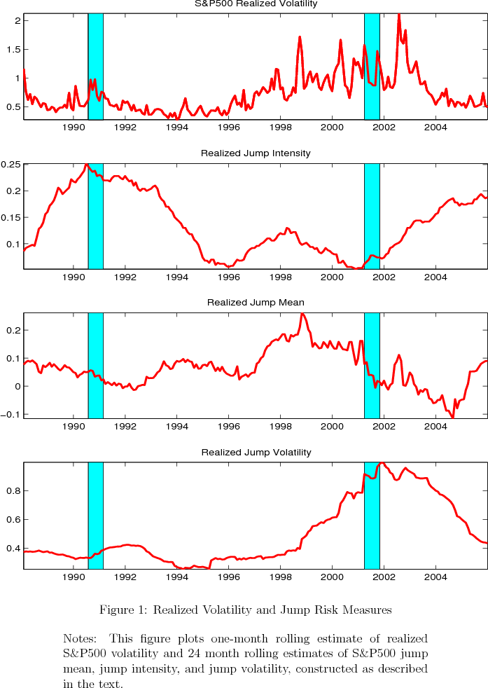
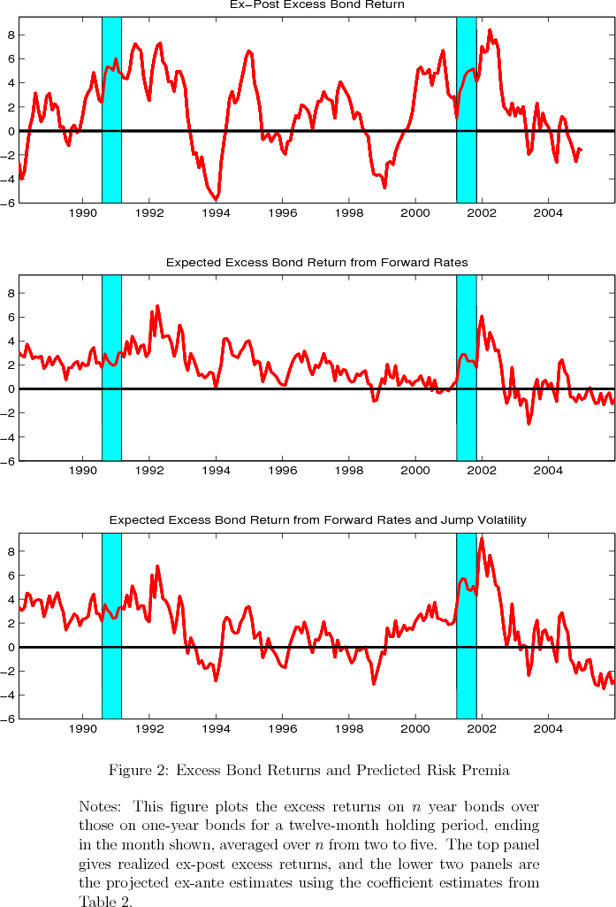
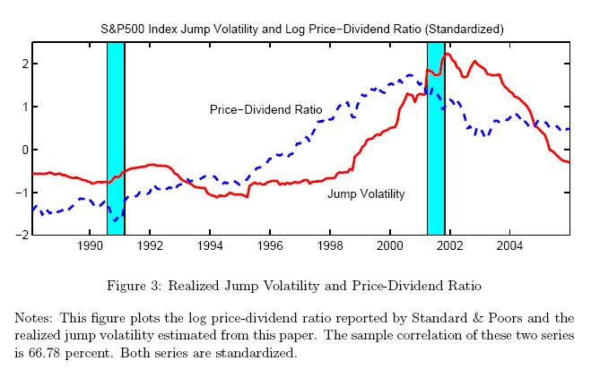
Footnotes
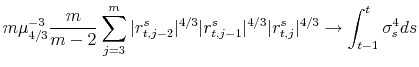 |
(7) |
with