Incorporating Vintage Differences and Forecasts into Markov Switching Models
Keywords: Recessions, Markov Switching Models
Abstract:
Introduction
This paper discusses extensions of standard Markov switching models that allow estimated probabilities to reflect parameter breaks at or close to the end of the sample, too close for standard maximum likelihood techniques to produce precise parameter estimates. The basic technique is a supplementary estimation procedure, bringing additional information to bear to estimate the statistical properties of the end-of-sample observations that behave differently from the rest; the additional information required is the historical values of the end-of-sample observations over the entire length of the time series employed. For example, assume that the first official estimate of GDP growth for a given quarter behaves differently than later-vintage estimates that have been revised a number of times, so a differential treatment of these vintages is appropriate. The techniques discussed here require the first release of GDP for every period in the sample under consideration. While this may sound like an onerous requirement, databases such as the Federal Reserve Bank of Philadelphia's Real-Time Dataset make it increasingly simple to meet.
The supplementary estimation techniques proposed here are computationally simple and highly intuitive. Many economists have computed the means and variances of variables of interest in recessions and expansions, defined by the NBER's start and end dates. One can interpret such a mean in recession periods as a weighted mean, with a weight of one assigned to periods designated as in recession, and a weight of zero assigned to other periods. The supplementary estimation procedure does essentially the same thing, taking weighted means and variances of the variables of interest - the time series of end-of-sample observations - with the weights being probabilities of recession determined by first-stage estimation of a Markov switching model, so the weights are not constrained to be either zero and one as implied by the NBER dating. Hamilton (1990) showed that such weighted averages are typically the maximum likelihood estimates of Markov switching model parameters; those results motivate the supplementary estimation procedure proposed here.
Section 2 of the paper discusses the crux of the basic problem in a general context, while section 3 outlines the solution the paper proposes. Section 4 works through three empirical applications in the context of estimating probabilities of recession in real time for the U.S. economy. The first application studies vintage differences in GDP growth, comparing the properties of the early-vintage estimates versus later-vintage estimates that have passed through annual and benchmark revisions. The supplementary estimation procedure employed has interesting implications, whether or not it is employed to modify standard Markov switching models: it serves as a useful diagnostic check on the early-vintage GDP estimates, asking whether they give useful information about the state of world.
The second application considers appending the officially-published GDP growth time series with forecasts of GDP growth. The forecasts used in this application are Greenbook forecasts produced by the staff of the Board of Governors of the Federal Reserve. These forecasts are released to the public with a lag of roughly five years, so this application is not meant to be of real-time use to anyone outside the Fed; it is merely meant to illustrate how a long history of forecasts may be used in conjunction with the paper's estimation techniques. The Board staff closely tracks the source data used to compute GDP growth, producing near-term GDP growth forecasts that are quite accurate. Updating probabilities of recession with these forecasts for the current quarter, instead of waiting to update until the official GDP data is released, has the potential to substantially increase the timeliness of the estimated probabilities.
The third application studies a bivariate Markov switching model estimated using GDP and gross domestic income (GDI), following Nalewaik (2007). The application incorporates vintage differences and appends each quarterly time series with forecasts based on higher-frequency indicators such as industrial production or unemployment insurance claims. This application uses real time data to track the performance of the model around the start of the 2001 recession, measuring the incremental impact of including the forecasts in the model. The results confirm that the forecasts do improve the timeliness of the model in recognizing the start of that recession.
Section 5 discusses alternative procedures for incorporating vintage differences and forecasts into Markov switching models, and points out reasons why the approach described here may be preferable. Section 6 concludes.
The Basic Problem
The standard Markov switching model outlined in Hamilton (1994) describes the vector of ![]() variables of interest
variables of interest
![]() for periods
for periods
![]() . Reviewing the standard model briefly, the joint density of
. Reviewing the standard model briefly, the joint density of
![]() conditional on the state of the world in the current period,
conditional on the state of the world in the current period, ![]() , is
, is
![]() . Past states of the world,
. Past states of the world,
![]() , have no effect on this conditional density. There exist
, have no effect on this conditional density. There exist ![]() states of
the world in the model, and let the estimated probability of state
states of
the world in the model, and let the estimated probability of state ![]() in period
in period
![]() , conditional on history though period
, conditional on history though period ![]() , be:
, be:
where
| (A.1) |
Given the
 |
The likelihood is a function of parameters
Each probability
![]() may be updated with respect to the current realization of
may be updated with respect to the current realization of
![]() as follows:
as follows:
| (A.2) |  |
Given
The model would be standard if period ![]() were the last period under consideration. However assume that there are
were the last period under consideration. However assume that there are ![]() additional time periods in the sample, and in these periods,
additional time periods in the sample, and in these periods,
![]() is not observed. A vector consisting of
is not observed. A vector consisting of ![]() substitute variables,
substitute variables,
![]() , is observed instead, and the conditional likelihoods of these variables are governed by
, is observed instead, and the conditional likelihoods of these variables are governed by
![]() rather than
rather than
![]() .
.
![]() could be a set of forecasts of
could be a set of forecasts of
![]() , or a set of preliminary estimates that will be revised in a significant way at a later date.
, or a set of preliminary estimates that will be revised in a significant way at a later date.
One can interpret this model as including a set of breaks in the parameters
![]() , occuring at a known point in the sample, with the transition matrix
, occuring at a known point in the sample, with the transition matrix ![]() remaining the same across the break. The log-likelihood function for this model is:
remaining the same across the break. The log-likelihood function for this model is:
 |
|||
| (A.3) |  |
We maintain the assumption that only the current state of the world affects the conditional densities of the
The issue in the applications considered below is small ![]() : there are too few observations to provide reliable estimates of
: there are too few observations to provide reliable estimates of
![]() through maximization of (3). In some cases of interest
through maximization of (3). In some cases of interest
![]() ; with more than one state of the world, sensible parameter estimates are obviously then infeasible. However assume that we have some supplementary information at our disposal: the
time series values of
; with more than one state of the world, sensible parameter estimates are obviously then infeasible. However assume that we have some supplementary information at our disposal: the
time series values of
![]() for all periods
for all periods
![]() . The estimation procedure outlined in the next section exploits this additional information to estimate
. The estimation procedure outlined in the next section exploits this additional information to estimate
![]() .
.
Supplementary Estimation of the Required End-Of-Sample Parameters
The first stage of the proposed procedure side-steps the small ![]() problem by maximizing (3) through period T, producing parameter estimates for
problem by maximizing (3) through period T, producing parameter estimates for
![]() ,
,
![]() and
and
![]() . Hamilton (1990) proves that the maximum likelihood estimates of
. Hamilton (1990) proves that the maximum likelihood estimates of
![]() satistfy:
satistfy:
| (A.4) |  |
where the derivatives are evaluated at
| (A.5) |  |
or the following criterion function:
| (A.6) |  |
With no regime-switching, so that
These facts motivate the second stage estimation procedure for
![]() . The proposed estimator of
. The proposed estimator of
![]() minimizes:
minimizes:
| (A.7) |  |
with first order conditions solving:
| (A.8) |  |
As noted earlier, these
With
![]() now in hand as well as
now in hand as well as
![]() ,
,
![]() and
and
![]() from the first stage, the usual recursion and smoothing techniques are applied to produce estimated probabilities through period
from the first stage, the usual recursion and smoothing techniques are applied to produce estimated probabilities through period
![]() , with the overall likelihood for the data as in (3). Probabilities
, with the overall likelihood for the data as in (3). Probabilities
![]() and
and
![]() through period
through period ![]() are produced in the standard way using
(1) and (2). For periods
are produced in the standard way using
(1) and (2). For periods
![]() , the updating changes to employ the likelihood of the end-of-sample data:
, the updating changes to employ the likelihood of the end-of-sample data:
| (A.9) |  |
Smoothed probabilities
This is the basics of the procedure. Before moving on to the empirical applications below, a couple of additional points should be noted. First, in some situations discussed below I conducted first stage estimation on the entire sample
![]() , imposing
, imposing
![]() for the last
for the last ![]() periods. Of course, in the second stage
periods. Of course, in the second stage
![]() was computed in the same manner as outlined above and so was allowed to differ from
was computed in the same manner as outlined above and so was allowed to differ from
![]() . This modification did not pose any problems to the basic procedure, and since the ratio
. This modification did not pose any problems to the basic procedure, and since the ratio
![]() was small in each case, the estimated
was small in each case, the estimated
![]() in the first stage largely reflect
in the first stage largely reflect
![]() rather than the
rather than the
![]() that govern the last
that govern the last ![]() observations. Second, it is clear that
the second-stage procedure can be repeated as many times as desired. Assume that the analyst suspects that
observations. Second, it is clear that
the second-stage procedure can be repeated as many times as desired. Assume that the analyst suspects that ![]() different types of data inhabit the last
different types of data inhabit the last
![]() observations of the sample under consideration, so the likelihood is of the form:
observations of the sample under consideration, so the likelihood is of the form:
 |
|||
 |
|||
 |
|||
 |
|||
| (A.10) |  |
This situation could be handled easily with first stage estimation as before, and
Empirical Applications
The first two applications considered below show estimation results using (8), and the third application shows estimation results and a sequence of smoothed probabilities around the start of the 2001 recesssion, using (9) and the algorithm of Kim (1994).
The U.S. Bureau of Economic Analysis (BEA) releases a number of different vintages of quarterly real GDP growth for any given quarter. The first three, the "advance", "preliminary", and "final" current quarterly estimates, are released about a month, two months, and three months after the end of the quarter, respectively. The "final" current quarterly estimates then stand until the summer, when the BEA releases an annual revision. Any given quarter is revised at its first three annual revisions (so 1999Q4 is revised at the 2000, 2001 and 2002 annual revisions), and then subsequently at benchmark revisions that occur approximately every five years. These revisions incorporate previously unavailable data to produce improved estimates, and the cumulative magnitude of all the revisions can be sizeable; see Mankiw and Shapiro (1986) and Fixler and Grimm (2002).
Assume that estimates that have passed through at least one annual revision are governed by a common set of parameters
![]() .2 Conditional on the state of the world,
the distribution of real GDP growth,
.2 Conditional on the state of the world,
the distribution of real GDP growth,
![]() , is Gaussian, so:
, is Gaussian, so:
 |
There are two states of the world, expansion (
The Markov transition matrix contains two parameters,
![\begin{displaymath}\left( \begin{array}{c} \pi_{t\vert t-1} 1-\pi_{t\vert t-1} \end{array} \right) = \left[\begin{array}{cc} p_{11} & 1-p_{22} 1-p_{11} & p_{22} \end{array}\right]\left(\begin{array}{c} \pi_{t-1\vert t-1} 1 - \pi_{t-1\vert t-1} \end{array} \right).\end{displaymath}](img87.gif) |
Estimating this model through period
| (A.11) |  |
||
 |
|||
 |
These are simple weighted averages computed using the smoothed probabilities as weights.
Consider the BEA's time series after a "final" current quarterly release. "Final" growth rates inhabit the last ![]() quarters of the sample - i.e. the quarters where data have not
passed through an annual revision yet. The distribution of "final" current quarterly GDP growth
quarters of the sample - i.e. the quarters where data have not
passed through an annual revision yet. The distribution of "final" current quarterly GDP growth
![]() is governed by
is governed by
![]() :
:
 |
The likelihood is as in (3).
Consider two examples of how
![]() may differ from
may differ from
![]() . First, assume each
. First, assume each
![]() is a noisy estimate of
is a noisy estimate of
![]() , so:
, so:
After first stage estimation gives
![]() ,
,
![]() and
and
![]() , application of (8) yields
, application of (8) yields
![]() by taking the same weighted averages as in (11):
by taking the same weighted averages as in (11):
| (A.12) |  |
||
 |
|||
 |
These conditional moments
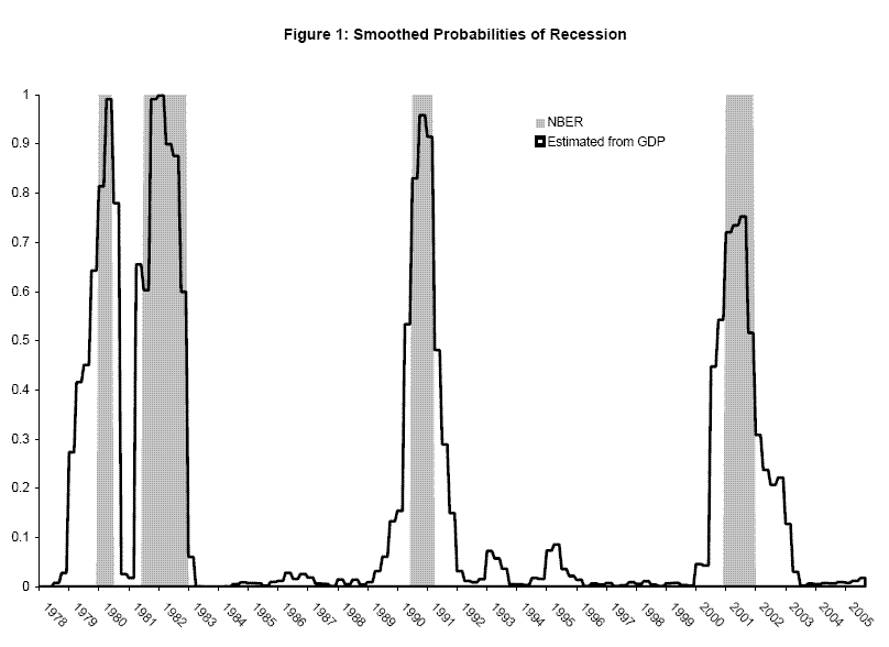
Having obtained each current quarterly growth rate of real GDP released by BEA since 1978Q1, my sample starts in that quarter. The two panels of table 1 show estimation results using (11) on the time series available at BEA's release of 2000Q3 and 2005Q4 data.3 Standard errors are below parameter estimates in parentheses. With a fairly short sample, the inclusion of an additional recession can swing around parameter estimates somewhat: the mean growth rate in recessions rises substantially when the relatively mild 2001 recession is included in the sample. Figure 1 shows smoothed probabilities from the second panel, the weights in (11) and (12). For the most part, these line up well with the NBER's start and end dates for recessions.4
The top panel of table 2 shows
![]() for the "final" current quarterly growth rates using (12) on the sample through 2005Q4. Comparing these parameters to those in the second panel of table 1, we see no
evidence that these "final" growth rates are noisy, as they have lower conditional variance than the revised growth rates. However they do pick up less of the variation in mean GDP growth arising from expansions (
for the "final" current quarterly growth rates using (12) on the sample through 2005Q4. Comparing these parameters to those in the second panel of table 1, we see no
evidence that these "final" growth rates are noisy, as they have lower conditional variance than the revised growth rates. However they do pick up less of the variation in mean GDP growth arising from expansions (
![]() ) and recessions (
) and recessions (
![]() ). The next two panels show results for the "preliminary" and "advance" growth rates. These estimates have smaller conditional variances than the "final" growth rates,
and they pick up slightly less of the mean growth differences across states.
). The next two panels show results for the "preliminary" and "advance" growth rates. These estimates have smaller conditional variances than the "final" growth rates,
and they pick up slightly less of the mean growth differences across states.
Overall it seems that treating these current quarterly growth rates as if they were heavily revised should entail little loss of accuracy in estimating probabilities of recession, as their conditional moments are not so dissimilar. However this will not necesarily be the case for other time series. For example Faust, Rogers, and Wright (2005) report that, for a number of G-7 countries, preliminary GDP growth rates contain a substantial amount of noise that is later revised away. In such cases accounting for vintage differences may be quite important in avoiding misleading inferences about whether these economies are in recession.
This application considers adding forecasts of GDP onto the end of the BEA's officially published time series. For example, at the end of March 1995, the BEA released its "final" current quarterly estimate of real GDP growth for 1994Q4. Plenty of data on 1995Q1 was available by the end of that
March, so a forecast of 1995Q1 based on that data would likely be reasonably accurate, and a probability of recession estimated using that forecast quite informative. However, in all likelihood, the statistical properties of the forecast will differ from the statistical properties of the officially
published data in prior quarters, as the officially published data are based on much more complete information. Assuming no the vintage differences, with
![]() for the forecast appended to the officially published time series, the likelihood is as in (3). Tacking on additional forecasts is an option as well - 1995Q2, 1995Q3, etc. The
likelihood will be as in (10), with
for the forecast appended to the officially published time series, the likelihood is as in (3). Tacking on additional forecasts is an option as well - 1995Q2, 1995Q3, etc. The
likelihood will be as in (10), with
![]() ,
,
![]() , if the published time series is appended with
, if the published time series is appended with ![]() forecasts.
forecasts.
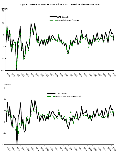
The staff of the Board of Governors of the Federal Reserve System produces its Greenbook forecasts of important economic aggregates before each of the eight meetings of the Federal Open Market Committee each year. These Greenbook forecasts have been released to the public through the end of 2000 as of the writing of this paper; this application analyzes the second Greenbook forecast produced each quarter, typically produced before FOMC meetings in March, June, September and December.5 The top panel of Figure 2 plots the Greenbook forecast for the current quarter, the dashed green line, with the "final" estimate of GDP growth rate for that quarter, typically released by BEA about three months later.6 The first panel of table 3 shows parameters estimated as in (12), with smoothed probabilities computed from the univariate GDP model using the time series available with the "final" 2000Q3 release. Comparing with the first panel of table 1, the mean growth rate in expansions is underestimated somewhat, but the mean growth rate in recessions is quite accurate, and the conditional variance is smaller than the conditional variance of GDP growth.
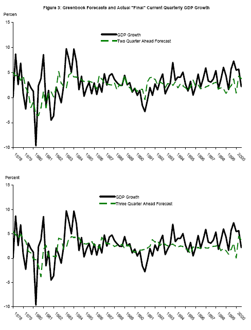
The second panel of Figure 2 shows one-quarter ahead Greenbook forecasts plotted again with the "final" growth rates (the one-quarter ahead forecast for 1995Q2 is reported in the March 1995 Greenbook, for example); the moments of these forecasts are shown in the second panel of Table 3. These one-quarter ahead forecasts pick up a considerable amount of business cycle variation in real GDP growth. The two- and three-quarter ahead forecasts are plotted in Figure 3, with estimated moments in the last two panels of Table 3. As expected, the gap between the recession and expansion mean growth rates diminishes at longer forecast horizons, as it becomes more difficult to forecast the state of the economy farther into the future. As this gap between the mean growth rates converges to zero, the updating (9) converges to no updating at all, as the forecasts are not informative about the future state of the world. To the extent that these forecasts are informative, though, the accuracy of the estimated probability of recession for the current quarter will be improved by smoothing using the information in forecasts for future quarters. So even if the goal is simply to estimate the probability of recession for the current quarter as accurately as possible, as opposed to estimating probabilities of recession for future quarters, forecasts may be informative. However it is clear from these tables that when appending published time series with forecasts several quarters ahead, the differential information content of the forecasts vis-a-vis official data needs to be taken into account when computing probabilities.
Before continuing, it should be mentioned that parameter stability is an obvious concern here: if the techniques used to produce Greenbook forecasts have changed over time, parameters estimated from historical forecasts may not be useful in evaluating the information content in current forecasts. This is probably more of a concern for the one- to three-quarter ahead forecasts than for forecasts of the current quarter, which are mostly a matter of carefully adding up publicly-released data that BEA uses to compile its estimates. This adding up is unlikely to have changed much over time.
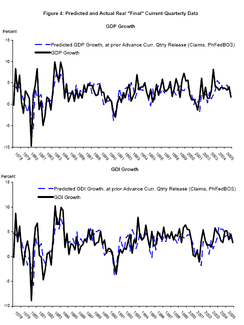
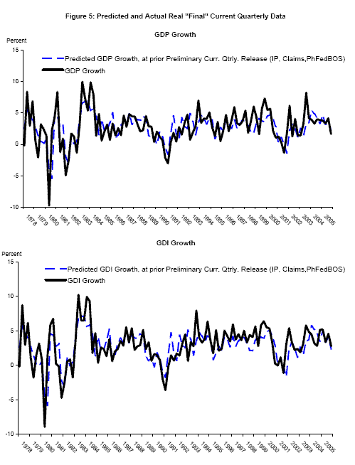
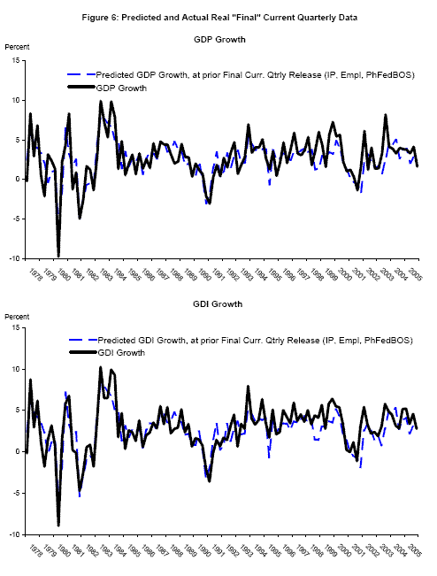
Nalewaik (2007) uses real time data to show that since 1978, the growth rate of gross domestic income (GDI), deflated by the GDP deflator, has done a better job recognizing recessions than has the growth rate of real GDP. That paper recommends a bivariate Markov switching model employing both GDP and GDI; this next application studies such a model, but goes further in accounting for vintage differences in the current quarterly estimates as in application 1, and appending each BEA time series with forecasts as in application 2. Probabilities of recession are computed at different BEA release dates, with the appended forecast employing one of three different information sets depending on whether the release is an "advance," "preliminary," or "final"; the information set contains variables typically available at the time of that type of release. The forecasts are for the current quarter only: for example at the time of BEA's "advance" current quarterly release of 1994Q4 data - January 1995 - the published time series is appended with a forecast for 1995Q1. These forecasts employ real time data on industrial production, employment, initial claims for unemployment insurance, and the Federal Reserve Bank of Philadelphia's Business Outlook Survey; details of forecast computation are in Appendix B. The predicted values from the forecasts, made at the time of the "advance," "preliminary," and "final" releases of the previous quarter's data, respectively, are plotted with "final" vintage data in Figures 4 to 6. These forecasts track the business cycle variation in real GDP and real GDI growth reasonably well.
A more thorough outline of the bivariate model can be found in Nalewaik (2007). Briefly, real GDP growth
![]() and real GDI growth
and real GDI growth
![]() are jointly normally distributed as:
are jointly normally distributed as:
![\displaystyle \left[\begin{array}{c} \Delta y_t^1 \Delta y_t^2 \end{array} \right] \sim N\left( \left[\begin{array}{c} \mu^1_{S_t} \mu^2_{S_t} \end{array}\right], \left[\begin{array}{cc} \left(\sigma^1\right)^2 & \sigma^{12} \sigma^{12} & \left(\sigma^2\right)^2 \end{array}\right]\right).](img116.gif)
|
The Markov transition matrix is as in application 1. Applying (4), the maximum likelihood estimates of the parameters of the model satisfy:
 |
|||
 |
|||
 |
 |
||
| (A.13) | 
|
As before, first stage maximum likelihood estimation of the model gives
![]() ,
,
![]() and
and
![]() . Applying (8) to each different vintage type or forecast at the end of the sample yields
. Applying (8) to each different vintage type or forecast at the end of the sample yields
![]() ; again these are simple weighted averages, using the same weighs as in (13):
; again these are simple weighted averages, using the same weighs as in (13):
| (A.14) |  |
 |
|
 |
 |
||
 |
 |
||

|
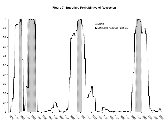
The top panel of Table 4 shows estimation results on the latest available time series as of the BEA's release of 2005Q4 data. The inclusion of real GDI growth in the Markov switching model has interesting effects discussed in more detail in Nalewaik (2007): the mean duration of recessions increases, leading to greater, actually positive, estimated mean growth rates in recessions. Figure 7 plots smoothed probabilities of recession from this model, and the more expansive definition of recessions is evident: the 1980 recession includes most of 1979, the 1990-1991 recession includes most of 1989, and the 2001 recession includes part of 2000 and all of 2002. With these smoothed probabilities as weights, real GDI has a smaller conditional variance than real GDP, and the gap between its high- and low-growth means is larger, implying that GDI is a better indicator of the state of the economy in this model.
The second panel of Table 4 shows
![]() for the "final" current quarterly growth rates computed from (14).7 Compared to the first panel, the parameters for real GDI growth are closer to those for real GDP growth: while the conditional variance remains smaller and the gap between the high- and low-growth means remains larger, these
advantages of real GDI as a signal of the state of the world are diminished. This is an important caveat to the results in Nalewaik (2007) showing that GDI outperforms GDP in recognizing the start of recessions.8
for the "final" current quarterly growth rates computed from (14).7 Compared to the first panel, the parameters for real GDI growth are closer to those for real GDP growth: while the conditional variance remains smaller and the gap between the high- and low-growth means remains larger, these
advantages of real GDI as a signal of the state of the world are diminished. This is an important caveat to the results in Nalewaik (2007) showing that GDI outperforms GDP in recognizing the start of recessions.8
The third and fourth panels of Table 4 show
![]() for the "preliminary" current quarterly growth rates. In the BEA's "preliminary" estimates for fourth quarters, corporate profits and a couple other components of
GDI are left missing because of poor data quality. These gaps were filled in with predictions as described in Appendix B. In the third panel, the time series of actual BEA releases is employed in (14), with predicted values substituting for actual releases only in fourth quarters; these parameters
are similar to those for the "final" current quarterly growth rates. The fourth panel shows results through 2005Q4 using the full time series of "preliminary" predicted values. The missing information on corporate profits is important, as the gap between the high- and low-growth means for GDI
growth contracts appreciably, and is now smaller than the gap for GDP.9 The last panel here shows shows
for the "preliminary" current quarterly growth rates. In the BEA's "preliminary" estimates for fourth quarters, corporate profits and a couple other components of
GDI are left missing because of poor data quality. These gaps were filled in with predictions as described in Appendix B. In the third panel, the time series of actual BEA releases is employed in (14), with predicted values substituting for actual releases only in fourth quarters; these parameters
are similar to those for the "final" current quarterly growth rates. The fourth panel shows results through 2005Q4 using the full time series of "preliminary" predicted values. The missing information on corporate profits is important, as the gap between the high- and low-growth means for GDI
growth contracts appreciably, and is now smaller than the gap for GDP.9 The last panel here shows shows
![]() for the "advance" current quarterly growth rates; these employ predicted values as they have the same missing components as fourth quarter "preliminary" releases,
so it is not surprising that these parameter estimates are similar to those in the prior panel.
for the "advance" current quarterly growth rates; these employ predicted values as they have the same missing components as fourth quarter "preliminary" releases,
so it is not surprising that these parameter estimates are similar to those in the prior panel.
Table 5 shows estimates of
![]() for the forecasts. For each of the three information sets we employ, there is some spread between the high- and low-growth means, confirming the visual evidence in
Figures 4-6 that the estimates track the business cycle variation in the data. These mean spreads are considerably smaller than those of the official BEA estimates, and the conditional variances are about half those reported in the top panel of table 4; a differential statistical treatment of the
forecasts when computing probabilities of recession seems appropriate in this case.
for the forecasts. For each of the three information sets we employ, there is some spread between the high- and low-growth means, confirming the visual evidence in
Figures 4-6 that the estimates track the business cycle variation in the data. These mean spreads are considerably smaller than those of the official BEA estimates, and the conditional variances are about half those reported in the top panel of table 4; a differential statistical treatment of the
forecasts when computing probabilities of recession seems appropriate in this case.
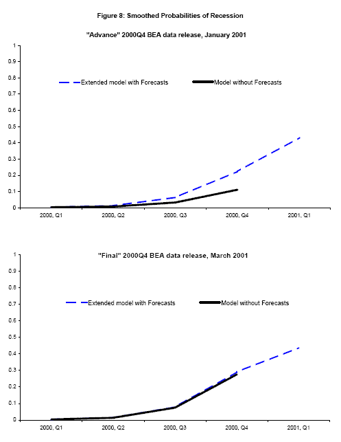
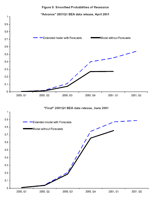
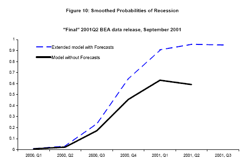
Figures 8-10, show smoothed probabilities of recession at selected BEA data releases around the start of the 2001 recession, computed using real time data and the paper's new estimation techniques. Each graph shows two time series of smoothed probabilities using data from an "advance" or a "final" release for a quarter, starting with the "advance" 2000Q4 release in the top panel of Figure 8. The solid line, in black, shows smoothed probabilities that account for vintage differences but employs no forecasts of GDP or GDI or its components. In "advance" releases where GDI is unavailable, the probability of recession for that quarter is updated with respect to GDP alone using the two-stage updating procedure described in Nalewaik (2007). The dashed line in blue shows smoothed probabilities that account for vintage differences and employ the forecasts as well, extending the time series forward one additional quarter.10 To get a better sense of the timing involved here, written in the label for each time series is the month when that data release occured.
The "advance" reading for 2000Q4 real GDP growth released in January 2001 was somewhat weak at 1.4![]() , leading to a probability of recession of about 10
, leading to a probability of recession of about 10![]() in the basic model with vintage differences but no forecasts. However the real time forecasts for 2001Q1 real GDP and GDI growth were weaker, predicting around-zero growth, as initial claims for unemployment
insurance had already started to shoot up and the Business Outlook Survey was extraordinarily weak. The model incorporating these forecasts shows estimated probabilities of recession of 43
in the basic model with vintage differences but no forecasts. However the real time forecasts for 2001Q1 real GDP and GDI growth were weaker, predicting around-zero growth, as initial claims for unemployment
insurance had already started to shoot up and the Business Outlook Survey was extraordinarily weak. The model incorporating these forecasts shows estimated probabilities of recession of 43![]() in 2001Q1 and 22
in 2001Q1 and 22![]() in 2000Q4.
in 2000Q4.
Little changes with the BEA's "preliminary" 2000Q4 release in February. The BEA's March 2001 "final" release brings the first published value of real GDI growth in 2000Q4, an anemic reading of 0.3![]() growth. The bottom panel of Figure 8 shows smoothed probabilities for this release: the weak value for GDI growth brings the 2000Q4 recession probability computed without forecasts up to about the same level as the probability computed with the aid of the forecasts.
growth. The bottom panel of Figure 8 shows smoothed probabilities for this release: the weak value for GDI growth brings the 2000Q4 recession probability computed without forecasts up to about the same level as the probability computed with the aid of the forecasts.
Moving to Figure 9, the April 2001 release of "advance" 2001Q1 real GDP growth, 2.0![]() , adds little information about whether or not the economy is in recession. The 2001Q2 forecasts
for GDP and GDI growth of 1.2
, adds little information about whether or not the economy is in recession. The 2001Q2 forecasts
for GDP and GDI growth of 1.2![]() and 1.4
and 1.4![]() are weaker, though again they
do not give an unambiguous signal of recession: the 2001Q2 probability of recession from the model with forecasts is 54
are weaker, though again they
do not give an unambiguous signal of recession: the 2001Q2 probability of recession from the model with forecasts is 54![]() , and the smoothed 2001Q1 probability is 45
, and the smoothed 2001Q1 probability is 45![]() , compared to the 27
, compared to the 27![]() probability of recession computed without the forecasts.
probability of recession computed without the forecasts.
The May 2001 "preliminary" release brings the BEA's first estimate of 2001Q1 real GDI growth, and its 0.1![]() value leads all the recession probabilities to jump up dramatically.
Smoothed probabilities from the June "final" release are similar; these are plotted in the bottom panel of Figure 9. Although these May and June releases bring the first clear evidence of recession whether or not the forecasts are employed, the forecasts allow the model to give a clearer warning
signal from January to April. Furthermore, Figure 10 shows probabilities of recession from the September "final" release of 2001Q2 data; it is notable that the probability of recession ticks down if we do not employ the forecasts, perhaps leading to some additional doubt about whether or not the
economy is in recession. If we employ the forecasts, however, there is little doubt, with estimated probabilities of recession in the first three quarters of the year consistently above 80
value leads all the recession probabilities to jump up dramatically.
Smoothed probabilities from the June "final" release are similar; these are plotted in the bottom panel of Figure 9. Although these May and June releases bring the first clear evidence of recession whether or not the forecasts are employed, the forecasts allow the model to give a clearer warning
signal from January to April. Furthermore, Figure 10 shows probabilities of recession from the September "final" release of 2001Q2 data; it is notable that the probability of recession ticks down if we do not employ the forecasts, perhaps leading to some additional doubt about whether or not the
economy is in recession. If we employ the forecasts, however, there is little doubt, with estimated probabilities of recession in the first three quarters of the year consistently above 80![]() .11
.11
These results indicate that even a simple, small-scale forecasting model for GDP and GDI growth one quarter ahead has the potential to significantly increase the timeliness of estimated probabilities of recession from basic Markov switching models. More comprehensive forecasting models could presumably do an even better job.
Alternative Procedures: Discussion
The multi-stage nature of the procedure outlined in this paper may be unappealing to some readers, and since the procedure relies on the accessibility of the full substitute time series
![]() for periods
for periods
![]() , an alternative would be to simply model the joint distribution of the time series of interest
, an alternative would be to simply model the joint distribution of the time series of interest
![]() with
with
![]() . Conditional on the state of the world, the distribution is
. Conditional on the state of the world, the distribution is
![]() . If
. If
![]() is a forecast, for example a linear function of other variables as in application 3 (so
is a forecast, for example a linear function of other variables as in application 3 (so
![]() ), use of a joint distribution such as
), use of a joint distribution such as
![]() is an option as well. As before,
is an option as well. As before,
![]() is unobserved for the last
is unobserved for the last ![]() periods of the sample, but this
poses no problems: the marginal distributions of
periods of the sample, but this
poses no problems: the marginal distributions of
![]() or
or
![]() can be employed to partially update probabilities in those last
can be employed to partially update probabilities in those last ![]() periods, with the remainder of the updating occuring later when
periods, with the remainder of the updating occuring later when
![]() is observed. An outline of this procedure is in Nalewaik (2007).
is observed. An outline of this procedure is in Nalewaik (2007).
When dealing with different vintages of estimates as in application 1, this option is clearly unappealing. After a revision to a quarterly estimate of GDP or GDI, the BEA essentially throws out the prior estimate; since the new revised estimate incorporates more information and is more accurate,
there is no reason to continue to examine the prior one. A model such as
![]() , then, would allow the probabilities of recession to depend on inferior data. For forecasts as in application 2, the
situation is analogous: once the variable to be forecast becomes known, the prior forecast typically becomes uninteresting. The forecast is clearly less accurate than the realization, so a model such as
, then, would allow the probabilities of recession to depend on inferior data. For forecasts as in application 2, the
situation is analogous: once the variable to be forecast becomes known, the prior forecast typically becomes uninteresting. The forecast is clearly less accurate than the realization, so a model such as
![]() would again allow the probabilities of recession to depend on inferior data. When it is feasible to decompose
the forecast into its component indicator variables
would again allow the probabilities of recession to depend on inferior data. When it is feasible to decompose
the forecast into its component indicator variables
![]() as in application 3, this remains true. GDP and GDI are the most comprehensive measures of the state of the economy. A model such as
as in application 3, this remains true. GDP and GDI are the most comprehensive measures of the state of the economy. A model such as
![]() places the indicators
places the indicators
![]() on an equal footing with GDP and GDI, giving them undue importance. For example, the results in application 3 show that the Federal Reserve Bank of Philadelphia's Business
Outlook Survey, a monthly diffusion index computed from a survey of mid-Atlantic-based manufacturers, is somewhat useful as an early indicator of the state of the economy before much other data on the period is available. Using such a survey for forecasting in that way seems reasonable, but placing
it on an equal footing with GDP or GDI in computing historical estimates of probabilities of recession is an entirely different matter.
on an equal footing with GDP and GDI, giving them undue importance. For example, the results in application 3 show that the Federal Reserve Bank of Philadelphia's Business
Outlook Survey, a monthly diffusion index computed from a survey of mid-Atlantic-based manufacturers, is somewhat useful as an early indicator of the state of the economy before much other data on the period is available. Using such a survey for forecasting in that way seems reasonable, but placing
it on an equal footing with GDP or GDI in computing historical estimates of probabilities of recession is an entirely different matter.
The multi-step nature of the procedure outlined in this paper has some appeal as well, as it allows the econometrician to handle an arbitrary number of different types of end-of-sample data at essentially zero computational cost. Often nothing more complicated than taking weighted means and variances is required to compute parameters estimated in stages beyond the first, although computation of standard errors is more complicated. Furthermore, the sequential estimation procedure may reduce parameter estimation error compared to such a case where all parameters are estimated jointly. Consider the time series after an "advance" or "preliminary" release in application 3, described as a bivariate model with three different types of data at the end of the sample. A joint distribution of these data, conditional on the state of the world, is:
Including all the cross covariance parameters between the different types of data, this model contains 55 parameters; simultaneous estimation of all these model parameters would likely lead to considerable parameter estimation error. Under the sequential estimation employed in application 3, no more than 10 parameters are estimated at any stage, and estimation of 24 of the cross covariance parameters is unnecessary.
While modelling the joint distribution
![]() is the most obvious alternative to the procedures outlined in this paper, some more complicated models have
been considered as well in attempting to incorporate supplementary information into Markov switching models. For example, Diebold, Lee and Weinbach (1994), Filardo (1994), Filardo and Gordon (1998) and others have modelled the parameters in the transition matrix
is the most obvious alternative to the procedures outlined in this paper, some more complicated models have
been considered as well in attempting to incorporate supplementary information into Markov switching models. For example, Diebold, Lee and Weinbach (1994), Filardo (1994), Filardo and Gordon (1998) and others have modelled the parameters in the transition matrix ![]() as functions of variables such as the
as functions of variables such as the
![]() in application 3, and Hamilton and Perez-Quiros (1996) have studied models where the state of the world shifts at different times for different variables. The concerns
discussed earlier, of estimated probabilities depending on inferior data, are less of a concern in these models, as the most comprehensive variables like GDP and GDI can be treated differently from the variables used to forecast them. However some concerns along these lines remain. In addition, the
added complexity of these models may reduce their robustness; for example Hamilton (2005) reports that models where the transition probabilities are functions of variables suffer from imprecise parameter estimates. A virtue of the procedures discussed in sections 2-4 is their simplicity; as the
different applications show, the simplicity and robustness of the estimation techniques allows them to handle complicated situations with relative ease.
in application 3, and Hamilton and Perez-Quiros (1996) have studied models where the state of the world shifts at different times for different variables. The concerns
discussed earlier, of estimated probabilities depending on inferior data, are less of a concern in these models, as the most comprehensive variables like GDP and GDI can be treated differently from the variables used to forecast them. However some concerns along these lines remain. In addition, the
added complexity of these models may reduce their robustness; for example Hamilton (2005) reports that models where the transition probabilities are functions of variables suffer from imprecise parameter estimates. A virtue of the procedures discussed in sections 2-4 is their simplicity; as the
different applications show, the simplicity and robustness of the estimation techniques allows them to handle complicated situations with relative ease.
Conclusions
This paper outlines techniques to account for differences between the statistical properties of different time series observations, in the context of the class of Markov switching models discussed in Hamilton (1994). It focuses on the case where a small number of observations at the end of the time series of interest exhibit statistical properties that are different from the rest, with this number being too small for standard maximum likelihood techniques to produce precise parameter estimates. The supplementary estimation techniques proposed here are computationally simple and highly intuitive: they are often simple generalizations of taking means and variances in the model's different states of the world.
Applications focused on a Markov switching model where the U.S. economy, as measured by GDP and its income-side counterpart GDI, switches between recession and expansion. One application shows how to treat differences across vintages of GDP, allowing early-vintage estimates that have not passed through many revisions to have different statistical properties than later-vintage estimates that have passed through a number of revisions. Perhaps more interesting, the techniques outlined here allow estimated probabilities of recession to reflect the information about the state of the economy embedded in forecasts. To do so, the forecasts are simply appended to the end of officially published time series, and the sample period is extended to include those additional periods. The statistical properties of the forecasts are, of course, allowed to differ in an arbitrary way from those of the official data, but to the extent that the forecasts are informative about the state of the economy in the forecast period, their incorporation will improve the accuracy of estimated probabilities of recession. Empirical results bear this out, as an application studying a bivariate model of GDP and GDI shows that the incorporation of forecasts improved the timeliness of the model in signalling that the economy was entering recession in early 2001.
|
|
|
|
|
|
|
|---|---|---|---|---|---|
| 4.05 | -1.41 | 7.60 | 0.95 | 0.73 | 1.00 |
| (0.38) | (1.52) | (1.23) | (0.03) | (0.18) | (1.55) |
|
|
|
|
|
|
|
|---|---|---|---|---|---|
| 3.91 | -0.40 | 7.04 | 0.95 | 0.76 | 1.00 |
| (0.45) | (1.47) | (1.06) | (0.03) | (0.16) | (1.55) |
|
|
|
|
|---|---|---|
| 3.48 | -0.15 | 6.06 |
| (0.39) | (1.43) | (0.88) |
|
|
|
|
|---|---|---|
| 3.46 | -0.23 | 5.67 |
| (0.39) | (1.48) | (0.84) |
|
|
|
|
|---|---|---|
| 3.27 | -0.22 | 5.24 |
| (0.37) | (1.43) | (0.77) |
|
|
|
|
|---|---|---|
| 3.02 | -1.53 | 4.53 |
| (0.30) | (1.40) | (0.74) |
|
|
|
|
|---|---|---|
| 2.61 | -0.32 | 3.59 |
| (0.29) | (0.77) | (0.53) |
|
|
|
|
|---|---|---|
| 2.59 | 0.73 | 2.33 |
| (0.21) | (0.65) | (0.36) |
|
|
|
|
|---|---|---|
| 2.60 | 1.32 | 1.72 |
| (0.17) | (0.53) | (0.27) |
|
|
|
|
|
|
|
|
|
|
|
|---|---|---|---|---|---|---|---|---|---|
| 4.18 | 4.36 | 0.63 | 0.26 | 7.20 | 6.03 | 4.96 | 0.93 | 0.85 | 1.00 |
| (0.34) | (0.34) | (0.67) | (0.64) | (1.03) | (0.90) | (0.85) | (0.03) | (0.08) | (1.28) |
Note: Moments of GDP have a 1 superscript, while moments of GDI have a 2 superscript.
|
|
|
|
|
|
|
|
|---|---|---|---|---|---|---|
| 3.72 | 3.96 | 0.69 | 0.67 | 6.11 | 5.71 | 5.52 |
| (0.30) | (0.30) | (0.69) | (0.68) | (0.82) | (0.79) | (0.78) |
Note: Moments of GDP have a 1 superscript, while moments of GDI have a 2 superscript.
|
|
|
|
|
|
|
|
|---|---|---|---|---|---|---|
| 3.71 | 3.92 | 0.67 | 0.65 | 5.84 | 5.47 | 5.29 |
| (0.29) | (0.30) | (0.69) | (0.66) | (0.78) | (0.77) | (0.75) |
Note: Moments of GDP have a 1 superscript, while moments of GDI have a 2 superscript.
|
|
|
|
|
|
|
|
|---|---|---|---|---|---|---|
| 3.68 | 3.67 | 0.68 | 1.07 | 5.82 | 5.13 | 4.20 |
| (0.29) | (0.28) | (0.72) | (0.60) | (0.77) | (0.68) | (0.63) |
Note: Moments of GDP have a 1 superscript, while moments of GDI have a 2 superscript.
|
|
|
|
|
|
|
|
|---|---|---|---|---|---|---|
| 3.49 | 3.67 | 0.65 | 0.99 | 5.35 | 5.12 | 4.21 |
| (0.29) | (0.29) | (0.70) | (0.62) | (0.71) | (0.68) | (0.62) |
Note: Moments of GDP have a 1 superscript, while moments of GDI have a 2 superscript.
|
|
|
|
|
|
|
|
|---|---|---|---|---|---|---|
| 3.41 | 3.51 | 0.47 | 0.45 | 3.36 | 3.75 | 3.54 |
| (0.23) | (0.25) | (0.58) | (0.61) | (0.44) | (0.48) | (0.46) |
Note: Moments of GDP have a 1 superscript, while moments of GDI have a 2 superscript.
|
|
|
|
|
|
|
|
|---|---|---|---|---|---|---|
| 3.46 | 3.63 | 0.90 | 0.84 | 2.84 | 3.23 | 3.02 |
| (0.21) | (0.23) | (0.56) | (0.60) | (0.24) | (0.25) | (0.24) |
Note: Moments of GDP have a 1 superscript, while moments of GDI have a 2 superscript.
|
|
|
|
|
|
|
|
|---|---|---|---|---|---|---|
| 3.33 | 3.69 | 0.70 | 0.87 | 2.93 | 3.29 | 3.10 |
| (0.22) | (0.23) | (0.54) | (0.57) | (0.20) | (0.21) | (0.20) |
Note: Moments of GDP have a 1 superscript, while moments of GDI have a 2 superscript.
To better understand equation (6), perhaps it would be useful to consider for a moment a problem quite different from the one at hand, one where the use of weighted averages is widespread. The problem is that of estimating the population mean and variance of a variable ![]() from a sample
from a sample
![]() of population members
of population members ![]() , and where individuals'
probabilities of selection into the sample differ. This problem is ubiquitous in the statistics literature on sampling; if the probabilities of selection are known, weights
, and where individuals'
probabilities of selection into the sample differ. This problem is ubiquitous in the statistics literature on sampling; if the probabilities of selection are known, weights ![]() for
each population member may be constructed, and the population mean and variance are estimated straightforwardly as:
for
each population member may be constructed, and the population mean and variance are estimated straightforwardly as:
| (A.1) |  and: and: |
||
| (A.2) |  |
Assume that
 |
Given this distributional assumption, we can work backward and ask what likelihood function produces formulas (A.2) and (A.3); the answer is:
| (A.3) |  |
This is a standard likelihood function except for the weights
The weights indicate that observations of type
Returning to the problem at hand and the likelihood (6), the similarity to (A.3) is evident. The major difference is that the Markov switching model implements a within-observation weighting; for the two-state case, the model assigns some fraction
![]() of observation
of observation ![]() to the expansion state, and the
remaining
to the expansion state, and the
remaining
![]() of observation
of observation ![]() to the recession state.
to the recession state.
Some components of GDI are missing in some BEA releases; before proceeding to the forecasts, this Appendix discusses computation of the predicted values for these missing components. Corporate profits is missing in the "advance" releases and fourth-quarter "preliminary" releases; to predict these, a time series consisting of the growth rates of "final" vintage corporate profits is regressed on the appropriate vintage (either "advance" or "preliminary" depending on which set of missing values we are trying to fill) of other available components of GDP and GDI.12 These explanatory variables are the growth rates of private consumption of fixed capital, and a couple of other cyclically sensitive variables - residential investment and personal consumption expenditures for durable goods.13 Since 1992, net factor income from abroad has been missing in the same releases as corporate profits, and from 1992 to 2002 net interest is missing in these releases as well. Predicted values for these two variables are computed in the same way in a similar fashion; for net factor income the explanatory variables are taxes on production and imports less subsidies and two lags of net factor income ("final" vintage), and for net interest the explanatory variables are one of its lags and employee compensation growth. These regressions are obviously somewhat ad hoc, and are just meant to be a rough attempt to fill in the missing data.
The forecasts are then constructed as follows. At the time of the "advance" release for quarter ![]() , almost a months worth of weekly data on new claims for unemployment insurance in
quarter
, almost a months worth of weekly data on new claims for unemployment insurance in
quarter ![]() is available. The Federal Reserve Bank of Philadelphia's Business Outlook Survey for the first month of the quarter is typically available as well; the explanatory variables
in the "advance" information set are the Survey's diffusion index measuring general business activity and the average value for claims.14 At the time of
the "preliminary" release for quarter
is available. The Federal Reserve Bank of Philadelphia's Business Outlook Survey for the first month of the quarter is typically available as well; the explanatory variables
in the "advance" information set are the Survey's diffusion index measuring general business activity and the average value for claims.14 At the time of
the "preliminary" release for quarter ![]() , initial claims and the Business Outlook Survey are available for the first two months of the quarter. In addition, a wide range data on the
first month of the quarter is available, including industrial production and non-farm payroll employment;15 employment growth added little explanatory
power, so I used the average of the two months of initial claims, the latest available Business Outlook Survey, and the latest available three month growth rate of industrial production as explanatory variables. One month of additional data on all these variables is available at the time of the
"final" release for quarter
, initial claims and the Business Outlook Survey are available for the first two months of the quarter. In addition, a wide range data on the
first month of the quarter is available, including industrial production and non-farm payroll employment;15 employment growth added little explanatory
power, so I used the average of the two months of initial claims, the latest available Business Outlook Survey, and the latest available three month growth rate of industrial production as explanatory variables. One month of additional data on all these variables is available at the time of the
"final" release for quarter ![]() ; the information set employed there is the latest three month growth rates of industrial production and payroll employment (growth rates from the middle
month of quarter
; the information set employed there is the latest three month growth rates of industrial production and payroll employment (growth rates from the middle
month of quarter ![]() to the middle month of quarter
to the middle month of quarter ![]() ), and the latest
available Business Outlook Survey, from the last month of quarter
), and the latest
available Business Outlook Survey, from the last month of quarter ![]() . A history of predicted values was stored from rolling regressions forecasting GDP and GDI using each information
set.16
. A history of predicted values was stored from rolling regressions forecasting GDP and GDI using each information
set.16
Although the in-sample ![]() values from the forecasting regressions over the full sample were not particularly high, ranging from 0.34 to 0.63, Figures 3 to 5 show that the predicted
values track the declines in GDP and GDI growth during the recessions in the sample. In addition, with the exception of an episode in mid-1995, these predicted values do not turn down in expansions.
values from the forecasting regressions over the full sample were not particularly high, ranging from 0.34 to 0.63, Figures 3 to 5 show that the predicted
values track the declines in GDP and GDI growth during the recessions in the sample. In addition, with the exception of an episode in mid-1995, these predicted values do not turn down in expansions.
Footnotes
