Evolving Macroeconomic Perceptions
and the Term Structure of Interest Rates*
JEL Codes: E43, E44, E47, G12
1 Introduction
Economic theory suggests that the term structure of interest rates at any moment ought to reflect agent's perceptions regarding the current state of the macroeconomy as well as its dynamic structure. The endogenous response of monetary policy to inflation and economic conditions provides a strong link between these factors and current and expected future short-term interest rates. And to the extent investor appetite for risk varies with business conditions, premia on long-term yields would also reflect current and expected business cycle developments.
In this light, the recent emergence of no-arbitrage term structure models with macroeconomic factors in fitting jointly the term structure of interest rates and macroeconomic dynamics of the U.S. economy, has been a welcome development in macroeconomics and finance. These models typically posit that the macroeconomy is governed by a simple fixed-coefficient dynamic structure and that agents know this structure and form expectations consistent with the model.
While such simple fixed-coefficients dynamic models have proven useful, many researchers also find that these models must be supplemented with additional latent factors and unobservable shocks to provide a satisfactory fit of yields across the spectrum of maturities. The key difficulty seems to be that such a fixed-coefficient model implies too tight a link between macro variables and bond yields by assuming that span the same information set and are linked to each other via a time-invariant functional form, an implication that has limited empirical support.
In this paper, we relax the restriction of a time-invariant relationship between macro variables and bond yields by allowing evolving perceptions regarding the dynamic structure of the economy. In particular, we posit that agents engage in real-time re-estimation and updating of a vector autoregression (VAR) model assumed to govern the dynamics of the macroeconomy and, in each period, form expectations based on the estimation results with data available during that period. In this manner, we obtain an anticipated-utility version of a no-arbitrage model of the term structure. We show that such a model generates forecasts about future path of the economy that are more consistent with the survey evidence and explore its role in improving the empirical performance of the macro finance models.
We estimate the model using real-time vintages of quarterly data and corresponding survey forecasts for inflation, output growth and the short-term interest rate from the Federal Reserve Bank of Philadelphia's survey of professional forecasters. To recover the evolution of perceptions about macroeconomic dynamics, in each quarter we estimate the VAR parameters that fit the historical data as well as the panel of survey forecasts in that quarter. We then use the recursive VAR estimates to fit our dynamic term structure model.
The main findings from this exercise can be summarized as follows. First, our results suggest significant deviations from the fixed-coefficient model-consistent benchmark model of expectations. Allowing for evolving perceptions regarding economic dynamics results in a significantly improved understanding of the evolution of expectations over time. Second, allowing for evolving macroeconomic expectations leads to large and economically significant improvement in the fit of the term structure, especially as the maturity lengthens. Contribution from an additional latent factor, albeit still large, become less important. Finally, survey forecasts provide useful information regarding the perceived future path of the economy and help improve both the in-sample fit and the out-of-sample forecasts of yields at the shorter end.
Our paper is related to the large literature on learning. Compared to models imposing rational expectations and a fixed known rule governing how the economy evolves over time, models in which agents have to infer in real time the structure of the economy appear to provide a better description of the inflation dynamics 1 and the monetary policy decision making process2, and generate forecasts about the future path of the economy that are more consistent with the survey evidence3. Term structure implications of learning have been examined by Cogley (2005) based on a two-yield-factor model and Piazzesi and Schneider (2006) in a consumption-based asset pricing framework. However, using yield curve factors in the former study prevents an examination of the economic driving forces behind interest rate variations; the relative few number of the factors in both studies also leads to a less than satisfactory fit of the cross section of yields.
Our paper builds on the rapidly expanding macro finance literature that examines bond pricing implications of New Keyesian models by superimposing either an exogenous specified or an endogenously derived pricing kernel.4 More recently, learning is incorporated into this type of models, where agents continuously update their beliefs regarding the central bank's inflation target (Kozicki and Tinsley (2001b,a), Dewachter and Lyrio (2006)) or the degree of monetary policy activism in general (Ang, Boivin, and Dong (2007)). In comparison, the current paper makes no a priori assumptions about the potential source of structural instabilities, but allows the agents to learn about all aspects--the drift, the slope coefficients and the conditional volatilities--of the economy. One paper that is most closely related to ours is Laubach, Tetlow, and Williams (2007), who approximate agents' changing expectations about the economy using a constant-gain VAR similar to ours and examine the term structure implications. However, they do not employ real-time information from survey data to estimate or evaluate the model as we do here.
Finally, a number of papers use survey information in term structure estimation. Kim and Orphanides (2006) show that incorporating additional information from survey forecasts of short-term interest rates help alleviate the small-sample problem when estimating a latent-factor term structure model. Pennacchi (1991) and D'Amico, Kim, and Wei (2007) use survey forecasts of inflation to identify expected inflation in a real term structure model, where most of the risk factors remain unobserved. In contrast, Chun (2007) directly employs the one-period ahead survey forecasts of the nominal short rate, real GDP growth and inflation as state variables, and assumes that investor expectations depend solely on their own lags with no feedback from subsequent realizations of the macro variables. His analysis also ignores information contained in the entire term structure of forecasts.
The rest of the paper is structured as follows. Section 2 motivates the paper and describes the data used in this study. We summarize the various models in Section 3 and review the estimation methodology in Section 4. The main empirical results are presented in Section 5 while Section 6 contains some further discussions. Finally, Section 7 concludes.
2 Data and Motivation
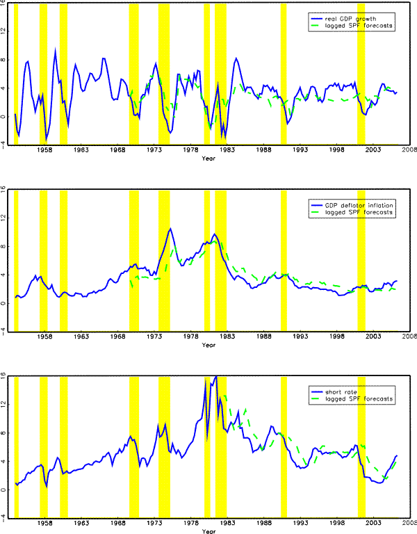
Figure 1 plots the 3-month nominal short rate, the final-vintage data on annual real GDP growth and annual GDP deflator inflation, together with the corresponding SPF forecasts four quarters ago, for the full sample of 1965Q4 to 2006Q2. Appendix A provides details on the data.
The macro term structure literature typically motivates the link between the term structure and the real economy by referring to a forward-looking monetary policy rule, in which the central bank judiciously selects an optimal short-term policy rate based on the predicted path of future economy. An important question is whether the presumed law of motion used in the empirical testing of the policy rule indeed generates forecasts consistent with investor expectations observed at the time of monetary policy decision. More specifically, under the further assumption that the economy evolves over time according to a fixed-coefficient VAR, these models have the future implication that the yield curve contain as much information about future macro variables as do current macro variables, since yields and the underlying macro state variables are flip sides of the same coin in such an economy.
Such a prediction can be easily tested. We estimate two predictive regressions for real GDP growth and inflation, where the explanatory variables are either the short rate, lagged real GDP growth and lagged inflation, or the 3-month, 1-year and 10-year nominal yields. When predicting real GDP growth, the two regressions become
andwhere
The results from these regressions based on the final-vintage data are reported in the first two panels of Table 1. As can be seen from the first panel, when predicting
next-quarter real GDP growth, the ![]() goes down from
goes down from ![]() using lagged macro
variables to
using lagged macro
variables to ![]() using yield curve variables alone. A more dramatic reduction in explanatory power is observed for quarterly inflation, as shown in the second panel, where the
using yield curve variables alone. A more dramatic reduction in explanatory power is observed for quarterly inflation, as shown in the second panel, where the ![]() falls from
falls from ![]() using macro regressors to
using macro regressors to ![]() using yield curve regressors.
using yield curve regressors.
At first sight, this seems to suggest that much of the yield curve variations are not related to macro variables, boding ill for any attempt to extract information about future economic condition from the current term structure or to explain yield curve variations using macro variables. A different interpretation, however, is that the assumption of a known fixed-coefficient data generating process is the reason for the disparate results. Indeed, ample empirical evidence that monetary policy practice and the structure of the macro economy may have shifted over time would suggest that such an assumption is unlikely to hold. Even if the true underlying structure of the economy were fixed over time, but economic agents had to estimate and discover this structure, beliefs would evolve over time as additional data were incorporated into the agents's discovery process. Depending on how real-time perceptions about the structure of the economy evolved over time, real-time expectations, and the term-structure of interest rates mirroring these expectations, would correspondingly differ. For instance, for any given history of economic growth rates and inflation, differences in the perceived persistence or the perceived long-term asymptotes of these variables could have vastly different implications for longer-term interest rates. Obviously, in such circumstances, yields continue to be driven by expectations about future macro variables, which are in turn linked to current macro variables in a time-varying fashion, suggesting that fixed-coefficient regressions like (1) and (2) are misspecified.
To examine the empirical validity of this conjecture, we re-run regressions (1) and (2) but replace the realized GDP growth and inflation by their SPF forecasts on the left hand side. As can be seen in Table 1, a different result emerges from this exercise. For example, the third panel of the table shows that using yield curve regressors alone, we can explain ![]() of the variations in the median SPF forecasts of next-period real GDP growth, much higher than the proportion explained when predicting realized real GDP growth. This is not surprising given that expectations contain less noises. More
encouragingly, however, this number is also higher than the proportion explained in a regression of future SPF forecasts of real GDP growth on lagged macro variables, which account for a slightly smaller
of the variations in the median SPF forecasts of next-period real GDP growth, much higher than the proportion explained when predicting realized real GDP growth. This is not surprising given that expectations contain less noises. More
encouragingly, however, this number is also higher than the proportion explained in a regression of future SPF forecasts of real GDP growth on lagged macro variables, which account for a slightly smaller ![]() of the observed variations in median SPF forecasts. Similarly, the last panel shows that the predictable proportion of the movement in SPF inflation forecasts goes down from around
of the observed variations in median SPF forecasts. Similarly, the last panel shows that the predictable proportion of the movement in SPF inflation forecasts goes down from around ![]() using macro variables to a lower yet still respectable
using macro variables to a lower yet still respectable ![]() using yield curve variables alone.
using yield curve variables alone.
Overall, Table 1 seems to suggest that yield curve contains important information about investor expectations about future macro variables; however, such a link is shrouded by a time-varying relationship between realized macro variables and their expected future values. In the rest of this paper, we introduce time-varying coefficients to the perceived law of motion of the economy, taking seriously the restriction that any forecast generated by the model should be a reasonably good approximation to the true investor expectations, as measured by survey forecasts, and examine the pricing implications for longer-term fixed-income assets.
3.1 Time-Varying VAR
At each quarter ![]() , investors observe last quarter's real GDP growth rate,
, investors observe last quarter's real GDP growth rate, ![]() , last quarter's inflation,
, last quarter's inflation,
![]() , the current 3-month nominal short rate,
, the current 3-month nominal short rate, ![]() , where the
subscript
, where the
subscript ![]() denotes quarter-
denotes quarter-
![]() values observed at quarter
values observed at quarter ![]() and reflects the time lag in macro
data releases. At time
and reflects the time lag in macro
data releases. At time ![]() , investors fit a VAR(2) to the vector of macro variables,
, investors fit a VAR(2) to the vector of macro variables,
![]() , based on a rolling sample of 40 quarters:
, based on a rolling sample of 40 quarters:
Investors update their VAR estimates in two steps. In the first step, they estimate the long-run mean of each variable as a discounted weighted average based on the rolling sample
Let
![]() be the extended state space and rewrite the VAR in the companion form in the usual way as
be the extended state space and rewrite the VAR in the companion form in the usual way as
![\begin{displaymath} \mu_{t}=\left[ \begin{array}[c]{c}% \mu_{z,t}\ 0 \end{array}\right] ,\text{ }\Phi_{t}=\left[ \begin{array}[c]{cc}% \Phi_{1,t} & \Phi_{2,t}\ I & 0 \end{array}\right] ,\text{ }\Sigma_{t}=\left[ \begin{array}[c]{c}% \Sigma_{z,t}\ 0 \end{array}\right] \end{displaymath}](img34.gif)
We assume that investors form expectations of future realizations of the macro variables based on current parameter estimates:
| (5) |
where
3.2 Term Structure
The nominal short rate is given by
![]() , where
, where ![]() is a selecting vector. Agents observe
current level of the short rate; their expectations about future short rates, on the other hand, depend on the current state variables as well as current parameter estimates.
is a selecting vector. Agents observe
current level of the short rate; their expectations about future short rates, on the other hand, depend on the current state variables as well as current parameter estimates.
The log nominal pricing kernel is specified in the usual fashion as
 |
(6) |
where
| (7) |
Two things are worth noting here. First, our price of risk loads on both lags of the macro variables albeit in a restricted fashion. This contrasts with the usual practice in the macro term structure literature of restricting the price of risk to load on current-period variables only.6 Second, we assume that term structure parameters,
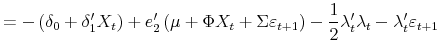
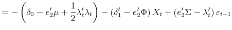
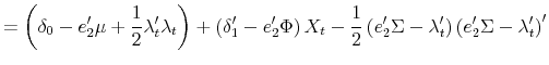
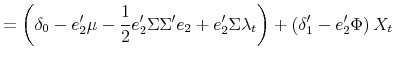
Given time-![]() VAR estimates, it is straightforward to show that the price of an
VAR estimates, it is straightforward to show that the price of an ![]() -period nominal bond is an exponential affine function of the state variables with time-varying coefficients:
-period nominal bond is an exponential affine function of the state variables with time-varying coefficients:
| (8) |
where
![\displaystyle =A_{n-1,t}+B_{n-1,t}\left[ \mu_{t}-\Sigma_{t}\left( \lambda _{0}+\lambda_{1}\varphi_{0,t}\right) \right] +\frac{1}{2}B_{n-1,t}\Sigma _{t}\Sigma_{t}^{\prime}B_{n-1,t}^{\prime}](img51.gif) |
||
with initial conditions
with coefficients
We also estimate some alternative models where the term structure is driven by one additional latent factor, ![]() , which is assumed to be conditionally uncorrelated with the macro factors
and follows the process
, which is assumed to be conditionally uncorrelated with the macro factors
and follows the process
![\displaystyle =\left[ \begin{array}[c]{c}% \lambda_{0}^{m} \lambda_{0}^{l}% \end{array} \right] =\left[ \begin{array}[c]{c}% \lambda_{0}^{m} 0 \end{array} \right] ,](img64.gif)
|
||
![\displaystyle =\left[ \begin{array}[c]{cc}% \lambda_{1}^{mm} & \lambda_{1}^{ml} \lambda_{1}^{lm} & \lambda_{1}^{ll}% \end{array} \right] =\left[ \begin{array}[c]{cc}% \lambda_{1}^{mm} & \lambda_{1}^{ml} 0 & 0 \end{array} \right] .](img66.gif) |
The price of risk parameters associated with shocks to the latent factor,
3.3 Summary of Models
Our main analysis will focus on three models. We start from a benchmark model (Model FC) where all VAR parameters are assumed to be time-invariant and are estimated once over the full sample using the final-vintage data, as commonly seen in the literature. The second model is our preferred model as specified above, which we hereafter refer to as Model TVC. Finally, we re-estimate Model TVC using SPF forecasts of macro variables as additional data inputs, which we will call Model TVC-S. Neither SPF forecasts of yields nor Blue Chip forecasts are used in the estimation.
For illustration purposes, we also estimate three alternative models. The first alternative model is motivated by Kozicki and Tinsley (2001b), who show that allowing time variations in the perceived inflation target is crucial for explaining the movement in the long end of the yield curve. To evaluate the relative contribution of time variations in the drifts versus in the rest of the parameters, we estimate an alternative model (Model PFC) where the drift terms, but not the slope or the volatility coefficients, vary over time. More specifically, we first estimate the time-varying drifts as the discounted weighted averages based on the last ten years of data, the same way as in Model TVC, and then estimate the slope and volatility coefficients using the demean data over the full sample. The second alternative model (Model TVC-L) is a variant of Model TVC, where we allow an additional latent factor to drive the term structure, as outlined in Section 3.2. To compare the role of such an additional latent factor when perceptions about macroeconomic dynamics are allowed to evolve over time versus the alternative fixed-coefficient assumption, we compare this model with Model FC-L, which adds a latent factor to Model FC.
Table 2 summarizes all models estimated in this paper.
4 Estimation
We use a two-step maximum likelihood procedure to estimate the model. The parameters ![]() can be partitioned into the parameters
can be partitioned into the parameters ![]() ,
, ![]() and
and ![]() that
govern the VAR dynamics (3), and the parameters
that
govern the VAR dynamics (3), and the parameters
![]() ,
,
![]() , and
, and
![]() in Models FC-L and TVC-L, that govern the term structure dynamics. In the first step, we estimate the VAR parameters
in Models FC-L and TVC-L, that govern the term structure dynamics. In the first step, we estimate the VAR parameters ![]() ,
, ![]() and
and ![]() based on either the final vintage (Model FC) or the current vintage (Model TVC) of data by standard OLS if no SPF forecasts are used in the estimation. If SPF forecasts are used, we estimate the model by maximizing the following log likelihood function
based on either the final vintage (Model FC) or the current vintage (Model TVC) of data by standard OLS if no SPF forecasts are used in the estimation. If SPF forecasts are used, we estimate the model by maximizing the following log likelihood function
 |
(10) |
where
In the second step, we estimate the price of risk parameters,
![]() and
and
![]() , and
, and ![]() if applicable, by maximizing the likelihood for observed
yields, holding the history of VAR parameter estimates,
if applicable, by maximizing the likelihood for observed
yields, holding the history of VAR parameter estimates, ![]() ,
, ![]() and
and
![]() , fixed from the first step. More precisely, at each time point
, fixed from the first step. More precisely, at each time point ![]() , we
observe yields on
, we
observe yields on ![]() zero coupon nominal bonds,
zero coupon nominal bonds,
![]() . we compute model-implied yields
. we compute model-implied yields
![]() based on the observed state variable and current parameter estimates, and find values of the parameters that solve the
problem
based on the observed state variable and current parameter estimates, and find values of the parameters that solve the
problem
One of the observed factors, the short rate, makes direct use of the yields
![]() , and is considered to be measured without any observation error. When estimating models with an extra latent factor, we make the additional assumption that the 7-year yield is
also observed without error. Other yields are functions of the state variables,
, and is considered to be measured without any observation error. When estimating models with an extra latent factor, we make the additional assumption that the 7-year yield is
also observed without error. Other yields are functions of the state variables, ![]() , according to the model pricing equation (9), and are treated as being measured with
small sampling errors. We assume that the sampling errors have mean zero and estimate their standard deviation
, according to the model pricing equation (9), and are treated as being measured with
small sampling errors. We assume that the sampling errors have mean zero and estimate their standard deviation ![]() in the second stage.
in the second stage.
5.1 Parameter Estimates
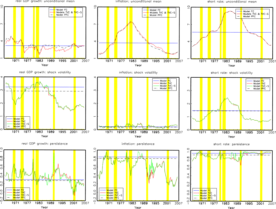
Table 3 reports the parameter estimates for Model FC, where all coefficients are held fixed throughout the sample. The unconditional moments of the VAR variables implied by this model are constant over time and are plotted as the blue line in Figure 2. The short rate is the most persistent factor among the three with an autocorrelation coefficient of 0.93, while the real GDP growth is the least persistent with an autocorrelation coefficient of 0.3. Unconditionally, the price of risk is negative (positive) for real GDP growth (inflation) shocks, with the puzzling implication that an asset with returns positively correlated with real GDP growth (inflation) shocks receives a negative (positive) risk premium on average. The price of real GDP growth (inflation) risks loads negatively (positively) on both the expected real GDP growth and the expected short rate, suggesting that investors are more sensitive to both types of shocks when the expected economic growth is relatively strong or when the expected short rate is high. In contrast, when the expected inflation is running above average, investors become more sensitive to real GDP growth shocks but less sensitive to inflation risks. The fitting errors in yields are much larger than in typical latent-factor models, especially at longer horizons.
Table 4 reports the parameter estimates for Model TVC, where VAR parameters are estimated on a rolling sample of 40 quarters and without using
additional information from SPF forecasts. The time-series average of the VAR parameter estimates reported here are quite similar to what we see in Model FC. The price of risk parameters, however, are quite different. Unconditionally, the price of risks is positive
(negative) for real GDP growth (inflation) shocks, which seems more plausible given that an average investors would prefer to hold an asset that has a higher return when the economy is weaker or when inflation is running high. The first two diagonal terms in the
![]() matrix is positive and negative, respectively, suggesting that investors become more sensitive to real GDP growth risks when the economy is expected to slow down and more
sensitive to inflation risks when inflation is expected to pick up. Fitting errors in yields of maturities of longer than two years are uniformly smaller than what we see in 3.
The biggest improvement is seen at the ten-year maturity with its fitting errors shrunk by more than 40%.
matrix is positive and negative, respectively, suggesting that investors become more sensitive to real GDP growth risks when the economy is expected to slow down and more
sensitive to inflation risks when inflation is expected to pick up. Fitting errors in yields of maturities of longer than two years are uniformly smaller than what we see in 3.
The biggest improvement is seen at the ten-year maturity with its fitting errors shrunk by more than 40%.
Finally, we introduce additional information from SPF forecasts and report the parameter estimates for Model TVC-S in Table 5. The fitting errors are larger than in Model TVC (Table 4) beyond the one-year maturity but still smaller than those in Model FC (Table 3).
Figure 2 plots the unconditional mean, shock volatility and persistence of the VAR variables as implied by the three models. Results based on Model FC are plotted in the blue lines and are constant over time. Results based on Models TVC and TVC-S (the red and green lines) are identical prior to 1986 and close to each other thereafter, and can exhibit sizable time variations. The top panels plots the unconditional means of the macro variables. As can be seen from the red lines, variations in the unconditional mean are more notable for inflation and the short rate, whose implied means rose from around 4% in early 1970's to about 7 % and 10%, respectively, in 1983, before declining to their current respective levels of about 1.5% and 4%. The middle panels plot the volatilities of shocks to these variables. The red and the green lines show that real GDP growth and short rate shocks exhibit more variations in their conditional volatilities, which have been on a downward path since mid 1980's, roughly coinciding with what is usually referred as the "Great Moderation." In comparison, inflation shock volatilities fluctuate within a relatively narrow band during the entire sample period. The bottom panels plot the first-order autocorrelation coefficient of each variable.7 Generally speaking, real GDP growth and inflation are less persistent today than in the 70's and 80's, while the persistence of the short rate is relatively unchanged.
5.2 Expectations of Future VAR Variables
Table 6 summarizes how model forecasts of future VAR variables differ from their survey counterparts. For all three models, we compute implied forecasts of real GDP growth, inflation and the 3-month short rate 1-, 2- and 4-quarters from now, and report the root mean squared differences between those forecasts and the corresponding survey counterparts, relative to a random walk benchmark. We also look at two measures of long-term expectations, including the expected 1-quarter variables 40 quarter hence and the expected average values five to ten years ahead. Panel A of the table looks at the entire sample period of 1965Q4 to 2006Q2. Introducing time-varying VAR coefficient in Model TVC results in larger discrepancies between model forecasts and survey forecasts at shorter horizons, but seems to approximate survey forecasts much better at forecasting horizons beyond one year. Not surprisingly, directly using information from survey forecasts in Model TVS-S further align the model-implied and survey forecasts at all horizons and all sample periods. The same pattern can be seen from the different sub-samples, shown in Panels B to D.
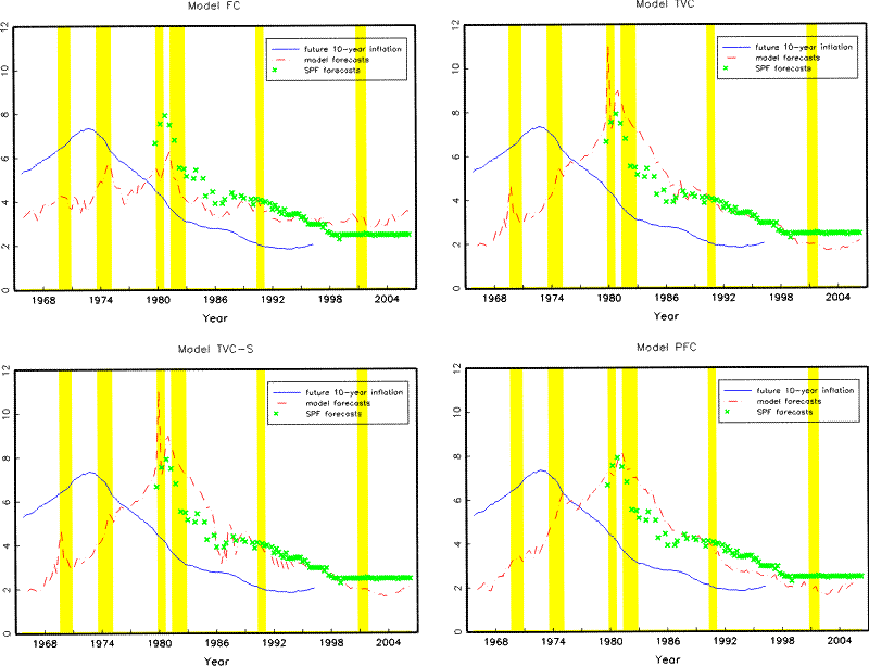
The first three panels in Figure 3 provide a visual comparison of the long-horizon inflation forecasts based on these models against the future realized value. A fixed-coefficient model like Model FC implies that state variables reverts to their time-invariant unconditional means fairly quickly and hence has trouble generating 10-year inflation expectations as variable as what we see from survey forecasts. In particular, the 10-year inflation forecasts during the early 1980s generated by this model only edged slightly higher and quickly came down to its average level, while survey forecasts from that period shot up and stay well above realized inflation for quite some time even as inflation moderated. Model TVC and TVC-S, neither of which uses survey information during this period, are able to match the substantial increase and the subsequent gradual decline of long-term inflation forecasts relatively well.
5.3 Expectations of Future Yields
A remaining question is whether a model that better describes agents' expectations about future macro economy also generates forecasts of future yields that are more consistent with the survey evidence. To answer this question, Table 7 compares model-implied and survey forecasts of 2- and 10-year yields and reports the root mean squared differences relative to a random walk model. Survey forecasts of longer-term yields are available only recently. In particular, forecasts of average 2- and 10-year yields during the next five to ten years are from the Blue Chip survey and are available since 1986Q1, while the SPF forecasts of 10-year yield is available since 1992Q1. Note that these forecasts are not used in estimating any of the models. Evidence based on this short sample period seems to suggest that allowing time variations in the VAR estimates in Model TVC generates forecasts of future yields that are closer to survey forecasts at the 10-year maturity but not at the shorter 2-year maturity. Consistent with Table 6 which suggests that survey information brings the biggest improve at the shorter end of VAR dynamics, the forecasts based on Model TVC-S also shows a smaller departure from survey forecasts at the shorter two-year maturity.
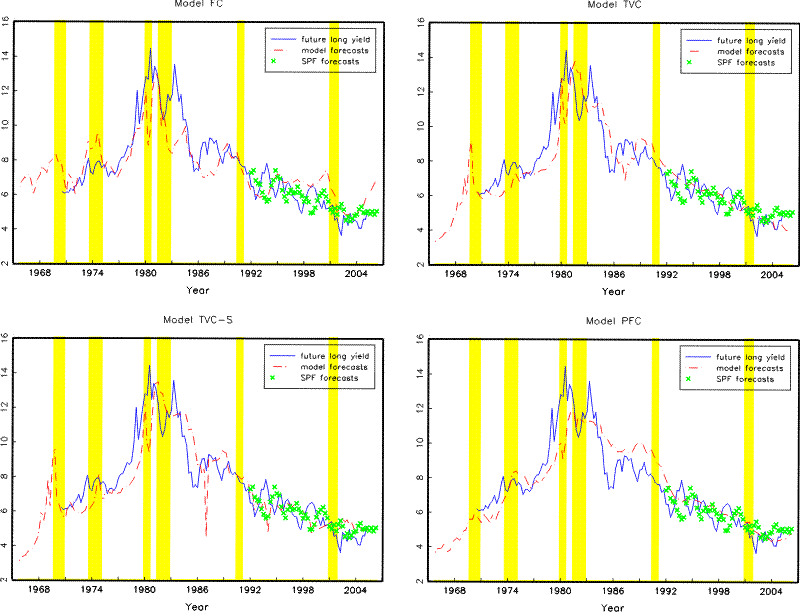
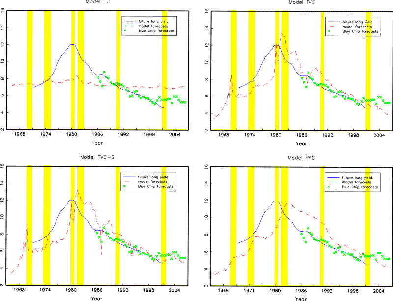
Figure 4 looks at model predictions for long-term interest rates in more details. The top left panel shows that Model FC consistently under-predicts the 10-year yield one year hence for much of the 1980's and almost completely misses the second spike in long yields around 1984. More recently, the model generates forecasts that lies consistently above future realized value throughout the late 1990's and predicts that the 10-year yield will rise quickly above 7% since the last monetary tightening cycle started in 2004, a trend that is absent both in the realized data and in SPF forecasts. In contrast, the top right and the bottom left panels show that Models TVC and TVC-S generate forecasts that correspond generally better with future realized values in all three cases and also with SPF forecasts in the last episode.
Moving towards even longer forecasting horizons, Figure 5 shows that Model FC generates almost no variations in 5- to 10-year ahead, 10-year yield expectations, whereas the Blue Chip survey forecasts declined from around 9% in mid 1980's to about 5.5% by mid 1990's. Both Models TVC and TVC-S are able to capture this decline; Model TVC-S also generates a long-horizon forecast of the 10-year yield that fluctuates about 5.5% since mid 1990's, consistent with the survey evidence.
5.4 Out-of-Sample Forecasting
Another way to test the model is too examine how well it performs in out-of-sample forecasting. It's conceivable that a model with more free parameters, such as the type of models with time-varying coefficients estimated in this paper, could fare better in sample but less well out of sample. To see whether this is the case, Table 8 reports the RMSEs in out-of-sample forecasting of VAR variables and long-term yields based on all three models, where both the VAR coefficients and the term structure parameter estimates are updated recursively based on the current sample, together with the corresponding SPF forecasts. Panel A of Table 8 shows that the two time-varying coefficient models (TVC and TVC-S) indeed perform slightly worse than the fixed-coefficient model (FC) in forecasting VAR variables out of sample, most notably for forecasting inflation. However, they are still comparable to the SPF forecasts.8
Turning to forecasting longer-term yields out of sample, Panel B shows that Model TVC outperforms model FC for maturities of five years and beyond and for horizons above one year, with the RMSE 65% lower when predicting 10-year yield two years hence. Introducing survey information on macro variables post 1986 in Model TVC-S mostly improves on the model's ability to predict the shorter end of the yield curve at the expense of a slightly worse performance when forecasting the long end of the yield curve, although it continues to outperform Model FC for the 10-year bond maturity and at the two-year forecasting horizon.
5.5 Term Structure Implications
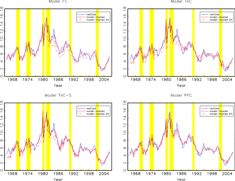
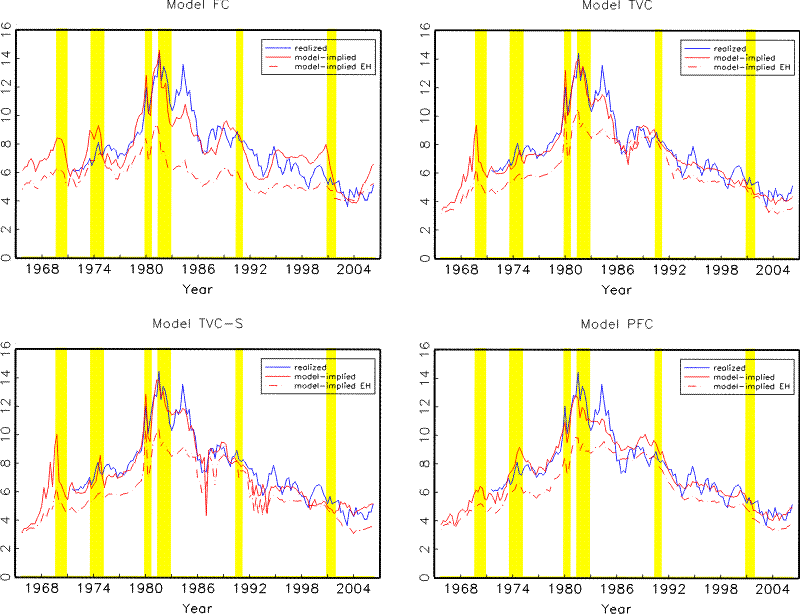
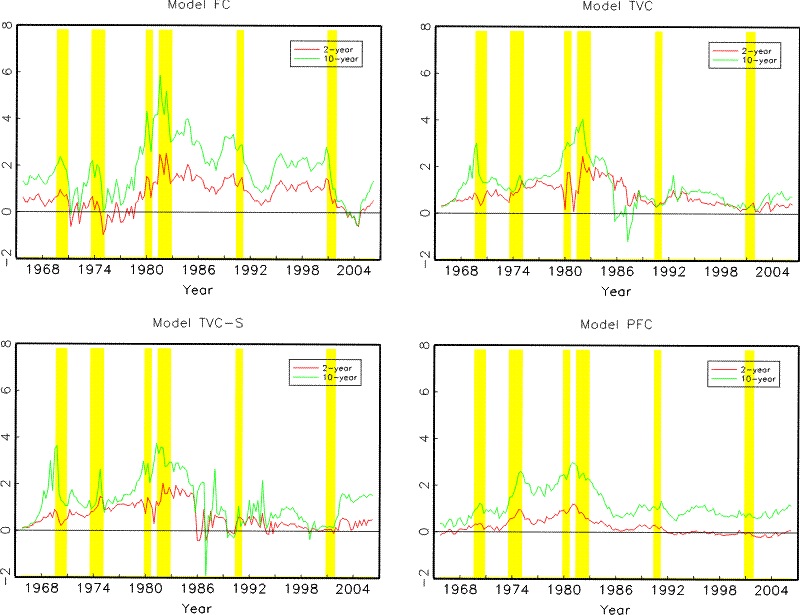
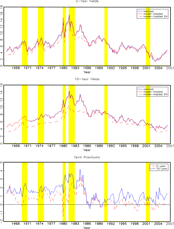
Allowing time variations in VAR parameters might lead to different term structure implications of the model, to which we now turn. Figures 6 and 7 plot the realized and model-implied 2- and 10-year nominal yields, together with the model-implied hypothetical yields when the Expectations Hypothesis (EH) holds. The corresponding term premiums are graphed in Figure 8.
Due to the persistent nature of interest rates, a stationary term structure model most likely will generate a long-term interest rate forecast in the near future that is close to its current value. Therefore, the top left panel of Figure 7 exhibits roughly the same pattern as seen in the top left panel of Figure 4: the ten-year yield as implied by Model FC lies below (above) its realized level in late 1980's (1990's) and is predicted to rise quickly since 2004 rather than fluctuating around the same level as seen in the data. The model-implied 10-year yield also bears too much similarity to the short rate. Comparing the red solid line and the red dashed line shows that the lower level of model-implied yields in the late 1980's largely reflects the expectation that the short rate will trend down and revert back to its lower long-term mean during the next ten years. On the other hand, Models TVC (top right panel) and TVC-S (bottom left panel) imply that the long-term mean of the short rate has shifted higher during this period, which pushes up the EH component and the total level of the long-term yield.
In comparison, the high level of model-implied 10-year yields in the 1990's as implied by Model FC is primarily due to an increase in the term premium rather than in the EH component, which in turn results from a positive correlation between the level of the short rate and the term premium (see Figure 8), as this model predicts that investors become more sensitive to both real GDP growth and inflation risks and demand a higher term premium as the short rate rises. In contrast, Models TVC and TVC-S imply that a higher short rate primarily acts to reduce risk premiums associated with all three shocks, as can be seen from the signs, leading to a lower term premium estimate in the 1990's, as shown in Figure 8, and a better fit with the realized data, as shown in Figure 7.
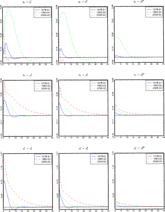
Figure 9 plots the impulse responses of 1-quarter, 1-year and 10-year yields to one standard deviation shocks to real GDP growth, inflation and the nominal short rate on three dates--1978Q1 and 1983Q1, two dates representing the periods immediately before and after the Volcker disinflation, and 2006Q2, the last data point in our sample--all based on Model TVC-S.9 Except for the negative yet imprecisely estimated contemporaneous response of the short rate, yields of all maturities respond to inflation shocks more strongly at the end of 1983 than in early 1978 or early 2006, consistent with the empirical evidence that the Fed combats inflation more vigorously post 1982.10 Shocks to the short rate also have the biggest effect on yields in late 1983, mainly reflecting a larger volatility of short rate shocks and a resulting larger term premium associated with short rate shocks during that period. In comparison, monetary policy during the most recent period is characterized by a response to real GDP growth shocks more aggressive than in previous periods.
Table 9 reports the results from an in-sample variance decomposition of yields of various maturities into components due to time-varying parameters, each state factor, and a remainder term.11 Model FC precludes variations in the parameters and attributes nearly all the variations in yields to movement in the short rate. In contrast, Models TVC and TVC-S attribute a considerable proportion of variations in yields to time variations in parameter estimates, especially at longer maturities. Short rate variations continue to explain most of the remaining movement, but changes in inflation now plays a slightly more important role in driving shorter-maturity yields.
6.1 Shifts in Mean versus Shifts in All Parameters
Kozicki and Tinsley (2001b) show that allowing time-varying endpoints is important for explaining the variations in long-term interest rates. To address the question whether the improvement in performance of Models TVC and TVC-S comes mainly from allowing a time-varying mean, we estimate an alternative model, Model PVC, where we allow time variations in the unconditional mean of the state variables but not in their persistence or volatilities. In particular, we model the shifting endpoints using a discounted weighted average with a rolling sample of 40 quarters and a quarterly gain of 98%, the same way as in Models TVC and TVC-S, but estimate the remaining VAR parameters once using the de-meaned final-vintage data over the full sample. The parameter estimates for this model are reported in Table 10, with the implied unconditional moments of VAR variables plotted as the black dashed lines in Figure 2. The unconditional means are close to those implied by Models TVC and TVC-S,12 while the shock volatilities and the persistence of the variables are close to those implied by Model FC.
The main implications of this model are shown in the bottom left panels of Figures 3 to 8. Here both inflation and the short rate slowly reverts to a time-varying mean that rises over time until around mid 1980s and then declines since then. As can be seen from Figures 3 and 4, the presence of these persistent yet time-varying asymptotes enables this model to capture most of the variations in long-horizon inflation expectations and long yield expectations since the corresponding SPF forecasts became available around 1980 and 1985, respectively. This model also fits two-year yield relatively well while attributing almost all the variations to the EH component, as can be seen from Figure 6. In addition, Figure 7 shows that it is able to capture the downward trend in the 10-year yields since early 1990s. Nevertheless, there are several episodes when this model provides a poor fit with the data. For example, it fails to match the magnitude of the two spikes in long yields during early and mid 1980s, as it by construction rules out the channel through which the rising volatilities of shocks to the real GDP growth and the nominal short rate lead the investors to demand a term premium.
Similarly, in the late 1980's, this model generates implied yields that are too high compared to the realized data, and overstates the subsequent decline in 10-year yield forecasts 5- to 10-year ahead when compared to the Blue Chip survey forecasts (Figure 5). During this period, the 3-month short rate is expected to revert to its unconditional mean of about 8.5% from a level of around 5%, which pushes up the EH component of 10-year yield, while the model-implied term premium is largely unchanged around that time. In comparison, Model TVC-S implies that the short rate is expected to mean-revert at a slower pace in early 1987 than in the previous period, leading to a slightly lower EH component. More importantly, both Model TVC and Model TVC-S imply that volatilities of real GDP growth shocks are revised down during this period, leading to a large reduction in the model-implied term premium in late 1980's.
Finally, repeating the out-of-sample forecasting exercise in Section 5.4 based on the PVC model produces RMSEs for 10-year yields that are uniformly larger than the TVC models discussed above. (Detailed results not shown here for brevity).
These results suggest that allowing for variation in the perceived means of macroeconomic variables is not sufficient to capture the role of evolving beliefs about the structure of the economy on the term structure of interest rates. Rather, the evolving beliefs about the nature of short-term macroeconomic dynamics, as reflected in slope parameters, must also be accounted for to improve our understanding of the term structure.
6.2 Contribution of Additional Latent Factor
So far we've shown that allowing time dependence in the perceived dynamics of underlying state variables helps improve the model's fit with observed longer-term yields; nonetheless, the yield fitting errors are still large compared to those from a typical latent-factor term structure model. In this section we examine whether we can further improve on Model TVC by introducing an additional unobserved factor, as outlined in Section 3.2. Recall that under this specification, the latent factor has no effect on how the macro variables, including the short rate, are perceived to evolve over time, but can affect longer-term yields by influencing the term premium.
The parameter estimates of the resulting model, Model TVC-L, are reported in Table 11. The yield fitting errors are much smaller compared to the corresponding model
without a latent factor, Model TVC, with the RMSE 40% lower at the 10-year maturity. This improvement can also be seen from the top two panels of Figure 10, which shows much smaller discrepancies between model-implied and realized yields at both the 2-year and the 10-year maturities. This better fit has to come through the term premium channel, as the perceived short rate process in this model is identical to that in Model TVC at each point in time. The bottom panel of Figure 10 plots the 2-year and 10-year term premiums. A comparison of these and the corresponding series implied by Model TVC, shown in the top right panel of Figure 8, shows that term premiums exhibit more high-frequency variations in this model, while their rise in the early 1980's and the subsequent decline assume a smaller magnitude. The
10-year term premium appears to be lower after 1985, when it fluctuates around 50 basis points, than before 1980, when it fluctuates around 150 basis points. The price of risk parameters,
![]() , loads positively and significantly on the latent factor for inflation and nominal short rate shocks, as shown in Table 11, implying that a more positive latent factor leads to a more negative price on inflation and nominal short rate risks and reduce the term premium. On the other hand, the loading of the price of real GDP growth risks on the latent
factor is not significantly different from zero.
, loads positively and significantly on the latent factor for inflation and nominal short rate shocks, as shown in Table 11, implying that a more positive latent factor leads to a more negative price on inflation and nominal short rate risks and reduce the term premium. On the other hand, the loading of the price of real GDP growth risks on the latent
factor is not significantly different from zero.
Comparing Panels E and B in Table 9 shows that the latent factor absorbs some of the variations previously attributed to time-varying coefficients, especially at longer maturities, and explains about one quarter of the variations in the 10-year yield. In comparison, when we re-estimate the benchmark model, Model FC, with an additional latent factor, (the FC-L model) the latent factor accounts for about 2/3 of the 10-year yield movement. At the short end of the yield curve, short rate variations continue to play a dominant role, while the latent factor explains about 15% of the 1-year yield movement.
These results suggest that although allowing for evolving beliefs regarding the dynamics of the macroeconomy cannot fully account for the explanatory power of latent factors in fixed-coefficient models, it does go a long way towards such an accounting.
7 Conclusion
In this paper we build a simple model that can accommodate the presence of evolving beliefs regarding macroeconomic dynamics, and examine their role in explaining the term structure of interest rates. In each period, agents re-estimate a VAR on real GDP growth, inflation and the nominal short-term interest rate, and use this recursively estimated VAR to form expectations. Using quarterly-vintages of real-time data and survey forecasts for the United States, we show that allowing for evolving macroeconomic perceptions in this manner generates predictions about the future path of the economy that are more consistent both with survey forecasts and with future realized values, relative to those from a benchmark model that imposes rational expectations and a fixed-coefficient VAR.
We then explore the role of the time-variation in beliefs regarding the structure of the economy for understanding the term-structure of interest rates. To that end, we price zero-coupon bonds of different maturities under the assumption that the investors' risk attitude is driven by expectations about the three macro variables in the following period. We find that when we allow for evolving beliefs about the macroeconomy, the resulting term structure model provides a better fit to the cross section of yields than the benchmark model--especially at longer maturities--and exhibits better performance in out-of-sample prediction of yield movements. Supplementing the data with information from survey forecasts during the first-step VAR estimation further reduces the discrepancies between model-implied forecasts and survey expectations not only for macro variables but also for bond yields at shorter maturities.
These findings demonstrate the usefulness of imposing additional discipline on the estimation of term structure models using information from survey forecasts. Existing work in a latent-factor setting has shown that such information can materially improve estimation of the expected future short rate and the expected excess returns on long-term bonds. In a macro term structure framework, it also helps to ensure that the underlying macroeconomic model correctly approximates the evolving nature of the process governing the formation of expectations about the outlook of the economy by bond market participants at the time when bond yields are observed.
Our main result is that allowing for time variation in the perceived mean, slope and conditional volatilities of macroeconomic variables can greatly facilitate our understanding of the linkages between the macroeconomy and the term structure. In addition, when we introduce an additional latent factor that is uncorrelated with the macro variables, we find that the latent factor accounts for a smaller portion of yield curve variations in our preferred time-varying model than in the benchmark fixed-coefficient model.
Accounting for evolving macroeconomic perceptions, as reflected by parameter variations in the perceived dynamic process governing the economy, can help reconcile the seemingly conflicting evidence that on the one hand, interest rates respond strongly to news about the key macroeconomic variables (as demonstrated by even studies), while on the other hand, yields appear to have low explanatory power for subsequent realizations of the macro variables.
In summary, we conclude that accounting for evolving macroeconomic perceptions is a critical step towards a better understanding of the term structure of interest rates in the context of macro-finance models.
Appendix
A. Data
Real-time data on seasonally adjusted real and nominal GDP is obtained from Federal Reserve Bank of Philadelphia's website for the sample period of 1954Q1 to 2006Q2.13 We construct the implied GDP deflator from these two series and measure inflation as the logarithm of quarterly changes in the implied GDP deflator.
Median SPF forecasts of 3-month T-Bill rate, nominal and real GDP level, GDP deflator and 10-year T-Bond yields are also obtained from Federal Reserve Bank of Philadelphia. SPF forecasts are available starting from 1968Q4 for nominal GDP and GDP deflator, from 1981Q3 for real GDP and 3-month T-Bill rates, and from 1992Q1 for 10-year T-Bond yields. We fill in real GDP forecasts for the period of 1968Q4 to 1981Q2 using forecasts of nominal GDP and GDP deflator. Survey participants forecast the level of each variable for the preceding, the current and the next four quarters, which allow us to construct quarterly growth rate forecasts for real GDP and GDP deflator for the current and the following four quarters. We also use five- to ten-year ahead forecasts of real GDP growth, GDP deflator inflation, and yields of maturities 3 months, 2 and 10 years from Blue Chip Economic Indicators, available twice a year in February and September between 1986Q1 and 2006Q2.14
Nominal yields for the maturities of 3-month and 1 to 5 years from 1965Q4 to 2006Q2 are obtained from CRSP. For longer maturities, we use 7- and 10-year yields based on a zero coupon nominal yield curve fitted at the Federal Reserve Board using the Svensson (1995) method, available since 1961Q3 for the 7-year maturity and since 1971Q4 for the 10-year maturity.15 We select yields at the end of the first month within each quarter to best approximate the release dates of real-time macro data as well as the SPF and Blue Chip forecasts.
B.1 Time-varying  ,
,  and
and 
Assuming that the price of an ![]() -period bond at time
-period bond at time ![]() is an exponential affine
function of the state variables
is an exponential affine
function of the state variables
![\displaystyle =E_{t}\left[ \exp\left( -r_{t}-\frac{1}{2}\lambda_{t}^{\prime}\lambda _{t}-\lambda_{t}^{\prime}\epsilon_{t+1}+A_{n-1,t}+B_{n-1,t}\widetilde{X}% _{t+1}\right) \right]](img90.gif) |
||
![\displaystyle =E_{t}\left[ \exp\left( -e_{1}^{\prime}\widetilde{X}_{t}-\frac{1}% {2}\lambda_{t}^{\prime}\lambda_{t}-\lambda_{t}^{\prime}\epsilon_{t+1}% +A_{n-1,t}+B_{n-1,t}\left( \widetilde{\mu}_{t}+\widetilde{\Phi}_{t}% \widetilde{X}_{t}+\widetilde{\Sigma}_{t}\epsilon_{t}\right) \right) \right]](img91.gif)
|
||
![\displaystyle =\exp\left[ -e_{1}^{\prime}\widetilde{X}_{t}+A_{n-1,t}+B_{n-1,t}\left( \widetilde{\mu}_{t}+\widetilde{\Phi}_{t}\widetilde{X}_{t}\right) +\frac{1}% {2}B_{n-1,t}\widetilde{\Sigma}_{t}\widetilde{\Sigma}_{t}^{\prime}% B_{n-1,t}^{\prime}-B_{n-1,t}\widetilde{\Sigma}_{t}\lambda_{t}\right]](img92.gif)
|
||
 |
||
| |
Therefore
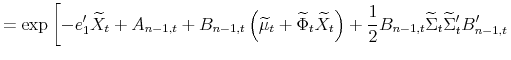
![\displaystyle =A_{n-1,t}+B_{n-1,t}\left[ \widetilde{\mu}_{t}-\widetilde{\Sigma }_{t}\left( \lambda_{0}+\lambda_{1}\varphi_{0,t}\right) \right] +\frac {1}{2}B_{n-1,t}\widetilde{\Sigma}_{t}\widetilde{\Sigma}_{t}^{\prime}% B_{n-1,t}^{\prime},](img97.gif) |
||
with initial conditions
B.2 Time-varying , Fixed and
Assuming that the price of an ![]() -period bond at time
-period bond at time ![]() is an exponential affine
function of the state variables
is an exponential affine
function of the state variables
![\displaystyle =E_{t}\left[ \exp\left( -r_{t}-\frac{1}{2}\lambda_{t}^{\prime}\lambda _{t}-\lambda_{t}^{\prime}\epsilon_{t+1}+A_{n-1}+B_{n-1}\widetilde{X}% _{t+1}+C_{n-1}\widetilde{\mu}_{t}\right) \right]](img102.gif) |
||
![\displaystyle =E_{t}\left[ \exp\left( -e_{1}^{\prime}\widetilde{Y}_{t}-\frac{1}% {2}\lambda_{t}^{\prime}\lambda_{t}-\lambda_{t}^{\prime}\epsilon_{t+1}% +A_{n-1}+B_{n-1}\left( \widetilde{\mu}_{t}+\widetilde{\Phi}\widetilde{X}% _{t}+\widetilde{\Sigma}\epsilon_{t}\right) +C_{n-1}\widetilde{\mu}% _{t}\right) \right]](img103.gif)
|
||
![\displaystyle =\exp\left[ -e_{1}^{\prime}\widetilde{X}_{t}+A_{n-1}+B_{n-1}\left( \widetilde{\mu}_{t}+\widetilde{\Phi}\widetilde{X}_{t}\right) +C_{n-1}% \widetilde{\mu}_{t}+\frac{1}{2}B_{n-1}\widetilde{\Sigma}\widetilde{\Sigma }^{\prime}B_{n-1}^{\prime}-B_{n-1}\widetilde{\Sigma}\lambda_{t}\right]](img104.gif)
|
||
 |
||
| |
where
 |
||
and
![\displaystyle =\left( \delta_{0}-\frac{1}{2}e_{2}^{\prime}\widetilde{\Sigma}% _{t}\widetilde{\Sigma}_{t}^{\prime}e_{2}-e_{2}^{\prime}\left[ \mu -\Sigma\left( \lambda_{0}+\lambda_{1}\varphi_{0}\right) \right] \right) +\left[ \delta_{1}^{\prime}-e_{2}^{\prime}\left( \Phi-\Sigma\lambda _{1}\varphi_{1}\right) \right] X_{t}%](img129.gif)
D. Variance Decomposition
The ![]() -quarter nominal yield is a function of underlying state variables
-quarter nominal yield is a function of underlying state variables
Its variance can be computed as
where we use the equality
The third term on the right hand side can be further decomposed into two components driven by macro and latent factors:
![\displaystyle \rho_{tvp}=\frac{var\left[ a_{n,t}\right] +2cov\left[ a_{n,t}% ,b_{n,t}E\left( X_{t}\right) \right] +var\left[ b_{n,t}E\left( X_{t}\right) \right] }{var\left[ y_{t}^{n}\right] },](img148.gif)
![\displaystyle \rho_{macro}=\frac{cov\left[ E\left( b_{n,t}\right) X_{t},E\left( b_{n,t}^{m}\right) X_{t}^{m}\right] }{var\left[ y_{t}^{n}\right] },](img149.gif)
![\displaystyle \rho_{latent}=\frac{cov\left[ E\left( b_{n,t}\right) X_{t},E\left( b_{n,t}^{l}\right) X_{t}^{l}\right] }{var\left[ y_{t}^{n}\right] },](img150.gif)
References
Ang, A., Boivin, J., and Dong, S. (2007). Monetary policy shifts and the term structure. Working Paper.
Ang, A. and Piazzesi, M. (2003). A no-arbitrage vector autoregression of term structure dynamics with macroeconomic and latent variables. Journal of Monetary Economics, 50(4):745-787.
Bekaert, G., Cho, S., and Moreno, A. (2004). New keynesian macroeconomics and the term structure. Working Paper.
Branch,W. A. and Evans, G.W. (2006). A simple recursive forecasting model. Economics Letters, 91(2):158-166.
Chun, A. L. (2007). Expectations, bond yields and monetary policy. Working Paper.
Clarida, R., Gali, J., and Gertler, M. (2000). Monetary policy rules and macroeconomic stability: Evidence and some theory. Quarterly Journal of Economics, 115(1):147-180.
Cogley, T. (2005). Changing beliefs and the term structure of interest rates: Cross-equation restrictions with drifting parameters. Review of Economic Dynamics, 8(2):420-451.
Cogley, T. and Sargent, T. J. (2002). Evolving post-world war II u.s. inflation dynamics. In Bernanke, B. S. and Rogoff, K., editors, NBER Macroecononic Annual 2001, volume 16, pages 331-373. MIT Press, Boston.
D'Amico, S., Kim, D. H., and Wei, M. (2007). Tips from TIPS: The informational content of Treasury Inflation-Protected Security prices. Working Paper.
Dewachter, H. and Lyrio, M. (2006). Learning, macroeconomic dynamics and the term structure of interest rates. Working Paper.
Gurkaynak, R. S., Sack, B., and Wright, J. H. (2006). The u.s. treasury yield curve: 1961 to the present. Finance and Economics Discussion Series 2006-28, Board of Governors of the Federal Reserve System.
H¨ ordahl, P., Tristani, O., and Vestin, D. (2006). A joint econometric model of macroeconomic and term structure dynamics. Journal of Econometrics, 131(1-2):405-444.
Kim, D. H. and Orphanides, A. (2006). Term structure estimation with survey data on interest rate forecasts. Working Paper.
Kozicki, S. and Tinsley, P. A. (2001a). Shifting endpoints in the term structure of interest rates. Journal of Monetary Economics, 47(3):613-652.
Kozicki, S. and Tinsley, P. A. (2001b). Term structure views of monetary policy under alternative models of agent expectations. Journal of Economic Dynamics and Control, 25(1-2):149-184.
Laubach, T., Tetlow, R. J., and Williams, J. C. (2007). Learning and the role of macroeconomic factors in the term structure of interest rates. Working Paper.
Orphanides, A. and Williams, J. C. (2005a). The decline of activist stabilization policy: Natural rate misperceptions, learning, and expectations. Journal of Economic Dynamics and Control, 29(11):1927-1950.
Orphanides, A. and Williams, J. C. (2005b). Inflation scares and forecast-based monetary policy. Review of Economic Dynamics, 8(2):498-527.
Pennacchi, G. G. (1991). Identifying the dynamics of real interest rates and inflation: Evidence using survey data. The Review of Financial Studies, 4(1):53-86.
Piazzesi, M. and Schneider, M. (2006). Equilibrium yield curves. In NBER Macroeconomics Annual 2006. MIT Press, Boston.
Rudebusch, G. and Wu, T. (2004). A macro-finance model of the term structure, monetary policy, and the economy. Working Paper.
Sargent, T. J. (1999). The Conquest of American Inflation. Princeton University Press, Princeton, N.J.
Stock, J. H. and Watson, M. W. (2007). Why has inflation become harder to forecast? Journal of Money, Creditand Banking, 39(s1):3-33.
Svensson, L. E. O. (1995). Estimating forward interest rates with the extended nelson & siegel method. Quarterly Review, Sveriges Riksbank, 3:13-26.
| Dependent Variable | constant (coefficient) |
|
|
||||
|---|---|---|---|---|---|---|---|
| 0.008 | -0.145 | 0.291 | -0.070 | 0.12 | |||
| (5.885) | (-1.321) | (4.385) | (-0.513) | ||||
| 0.008 | -1.322 | 1.075 | 0.105 | 0.07 | |||
| (3.011) | (-1.988) | (1.323) | (0.317) | ||||
| 0.001 | 0.108 | 0.013 | 0.766 | 0.73 | |||
| (1.060) | (2.728) | (0.562) | (15.672) | ||||
| 0.007 | 0.644 | 0.220 | -0.526 | 0.39 | |||
| (3.777) | (1.533) | (0.428) | (-2.513) | ||||
|
|
0.009 | -0.318 | 0.228 | -0.026 | 0.30 | ||
|
|
(8.406) | (-4.478) | (4.472) | (-0.301) | |||
|
|
0.008 | -1.995 | 1.612 | 0.127 | 0.32 | ||
|
|
(4.523) | (-4.922) | (3.257) | (0.628) | |||
|
|
0.000 | 0.205 | 0.017 | 0.638 | 0.82 | ||
|
|
(0.365) | (6.105) | (0.683) | (15.860) | |||
|
|
0.005 | 0.551 | 0.214 | -0.340 | 0.52 | ||
|
|
(3.300) | (1.664) | (0.531) | (-2.063) |
 from regressions of realized quarterly real GDP growth (
 ,
,  and
and | Model | VAR: Mean | VAR: Slope | VAR: Use survey | VAR: Data Vintage | Latent factor |
|---|---|---|---|---|---|
| FC | fixed | fixed | N | final data | N |
| TVC | discounted rolling average | rolling | N | real-time data | N |
| TVC-S | discounted rolling average | rolling | Y | real-time data | N |
| PFC | discounted rolling average | fixed | N | final data | N |
| TVC-L | discounted rolling average | rolling | N | real-time data | Y |
| FC-L | fixed | fixed | N | final data | Y |
| TVC-S-L | discounted rolling average | rolling | Y | real-time data | Y |
| GDP growth | 3.581 | 0.221 | 0.074 | 0.939 | 0.045 | -0.239 | -1.049 |
| GDP growth (standard deviation) | (0.218) | (0.017) | (0.005) | (0.043) | (0.004) | (0.011) | (0.033) |
| inflation | 0.132 | 0.006 | 0.516 | 0.097 | 0.017 | 0.347 | -0.043 |
| inflation (standard deviation) | (0.149) | (0.000) | (0.019) | (0.014) | (0.002) | (0.012) | (0.004) |
| short rate | 0.086 | 0.047 | 0.184 | 0.846 | 0.006 | -0.065 | 0.031 |
| short rate (standard deviation) | (0.138) | (0.004) | (0.021) | (0.022) | (0.000) | (0.005) | (0.001) |
|
|
|
|
|
||||
|---|---|---|---|---|---|---|---|
| GDP growth | 3.243 | -0.980 | -0.995 | -0.248 | -0.989 | ||
| GDP growth (standard deviation) | (0.227) | (0.072) | (0.019) | (0.015) | (0.071) | ||
| inflation | -0.192 | 1.142 | 2.882 | 0.072 | -0.104 | 0.574 | |
| inflation (standard deviation) | (0.112) | (0.099) | (0.558) | (0.003) | (0.016) | (0.031) | |
| short rate | 0.116 | 0.096 | 0.925 | -1.519 | 0.340 | 0.265 | -0.079 |
| short rate (standard deviation) | (0.090) | (0.088) | (0.237) | (0.071) | (0.013) | (0.016) | (0.009) |
| 1-yr | 2-yr | 3-yr | 4-yr | 5-yr | 7-yr | 10-yr |
|---|---|---|---|---|---|---|
| 0.453 | 0.669 | 0.791 | 0.894 | 0.959 | 1.037 | 1.093 |
| (0.050) | (0.108) | (0.028) | (0.253) | (0.056) | (0.039) | (0.177) |
| GDP growth | 6.844* | 0.105* | -0.389* | 1.200* | 0.037* | -0.300* | -1.514* |
| GDP growth (standard deviation) | (4.098)* | (0.179)* | (0.393)* | (0.719)* | (0.126)* | (0.533)* | (0.652)* |
| inflation | 0.423* | 0.020* | 0.375* | 0.201* | -0.042* | 0.028* | 0.128* |
| inflation (standard deviation) | (1.468)* | (0.075)* | (0.156)* | (0.359)* | (0.046)* | (0.192)* | (0.349)* |
| short rate | 0.719* | 0.026* | 0.218* | 1.003* | 0.024* | -0.063* | -0.242* |
| short rate (standard deviation) | (0.672)* | (0.055)* | (0.198)* | (0.264)* | (0.048)* | (0.135)* | (0.180)* |
 is divided by 400.
|
|
|
|
|
||||
|---|---|---|---|---|---|---|---|
| GDP growth | 2.509* | -1.256 | 0.399 | 0.300 | -0.100 | ||
| GDP growth (standard deviation) | (0.715)* | (0.152) | (0.043) | (0.049) | (0.026) | ||
| inflation | -0.117* | 0.954* | -0.756 | 0.019 | -0.023 | 0.102 | |
| inflation (standard deviation) | (0.180)* | (0.375)* | (0.082) | (0.020) | (0.024) | (0.015) | |
| short rate | 0.120* | 0.041* | 0.711* | 0.288 | -0.225 | -0.223 | 0.114 |
| short rate (standard deviation) | (0.097)* | (0.159)* | (0.455)* | (0.060) | (0.012) | (0.014) | (0.008) |
is divided by 400.| 1-yr | 2-yr | 3-yr | 4-yr | 5-yr | 7-yr | 10-yr |
|---|---|---|---|---|---|---|
| 0.582 | 0.678 | 0.683 | 0.677 | 0.679 | 0.673 | 0.635 |
| (0.058) | (0.196) | (0.358) | (0.314) | (0.376) | (0.181) | (0.084) |
is divided by 400.| GDP growth | 6.482* | 0.111* | -0.370* | 1.217* | 0.038* | -0.254* | -1.513* |
| GDP growth (standard deviation) | (4.325)* | (0.181)* | (0.400)* | (0.732)* | (0.121)* | (0.521)* | (0.654)* |
| inflation | 0.417* | 0.020* | 0.373* | 0.200* | -0.042* | 0.029* | 0.129* |
| inflation (standard deviation) | (1.467)* | (0.074)* | (0.156)* | (0.357)* | (0.047)* | (0.195)* | (0.348)* |
| short rate | 0.635* | 0.026* | 0.220* | 1.008* | 0.022* | -0.060* | -0.237* |
| short rate (standard deviation) | (0.622)* | (0.056)* | (0.198)* | (0.260)* | (0.047)* | (0.137)* | (0.186)* |
is divided by 400.|
|
|
|
|
||||
|---|---|---|---|---|---|---|---|
| GDP growth | 2.509* | -1.240 | 0.234 | 0.237 | -0.061 | ||
| GDP growth (standard deviation) | (0.780)* | (0.120) | (0.033) | (0.037) | (0.021) | ||
| inflation | -0.115* | 0.924* | -0.521 | -0.004 | -0.138 | 0.130 | |
| inflation (standard deviation) | (0.184)* | (0.447)* | (0.054) | (0.015) | (0.017) | (0.011) | |
| short rate | 0.126* | 0.037* | 0.354* | 0.723 | -0.183 | -0.181 | 0.049 |
| short rate (standard deviation) | (0.094)* | (0.161)* | (0.770)* | (0.035) | (0.008) | (0.009) | (0.005) |
is divided by 400.| 1-yr | 2-yr | 3-yr | 4-yr | 5-yr | 7-yr | 10-yr |
|---|---|---|---|---|---|---|
| 0.573 | 0.670 | 0.700 | 0.729 | 0.745 | 0.775 | 0.717 |
| (0.051) | (0.166) | (0.325) | (0.338) | (0.327) | (0.154) | (0.083) |
is divided by 400.| Horizon | Model FC: GDPG | Model FC: inflation | Model FC: 3m yld |
Model TVC: GDPG | Model TVC: inflation | Model TVC: 3m yld |
Model TVC-S: GDPG | Model TVC-S: inflation | Model TVC-S: 3m yld |
|---|---|---|---|---|---|---|---|---|---|
| 1 | 0.671 | 0.769 | 1.266 | 0.752 | 0.809 | 1.799 | 0.685 | 0.788 | 1.675 |
| 2 | 0.686 | 0.806 | 1.373 | 0.767 | 0.939 | 1.443 | 0.665 | 0.917 | 1.163 |
| 4 | 0.586 | 0.787 | 1.311 | 0.759 | 1.015 | 1.163 | 0.670 | 1.002 | 0.904 |
| 40 | n/a | 0.980 | n/a | n/a | 0.806 | n/a | n/a | 0.811 | n/a |
| 20-40 | 0.722 | 0.599 | 0.309 | 0.280 | 0.326 | 0.531 | 0.286 | 0.265 | 0.410 |
| Horizon | Model FC: GDPG | Model FC: inflation | Model FC: 3m yld |
Model TVC: GDPG | Model TVC: inflation | Model TVC: 3m yld |
Model TVC-S: GDPG | Model TVC-S: inflation | Model TVC-S: 3m yld |
|---|---|---|---|---|---|---|---|---|---|
| 1 | 0.645 | 0.802 | 0.501 | 0.726 | 0.733 | 0.718 | 0.726 | 0.733 | 0.718 |
| 2 | 0.691 | 0.801 | 0.695 | 0.780 | 0.870 | 0.504 | 0.780 | 0.870 | 0.504 |
| 4 | 0.571 | 0.768 | 1.011 | 0.823 | 1.027 | 0.717 | 0.823 | 1.027 | 0.717 |
| 40 | n/a | 2.620 | n/a | n/a | 1.220 | n/a | n/a | 1.220 | n/a |
| 20-40 | n/a | n/a | n/a | n/a | n/a | n/a | n/a | n/a | n/a |
| Horizon | Model FC: GDPG | Model FC: inflation | Model FC: 3m yld |
Model TVC: GDPG | Model TVC: inflation | Model TVC: 3m yld |
Model TVC-S: GDPG | Model TVC-S: inflation | Model TVC-S: 3m yld |
|---|---|---|---|---|---|---|---|---|---|
| 1 | 0.757 | 0.686 | 1.391 | 0.877 | 1.129 | 2.100 | 0.656 | 1.071 | 1.978 |
| 2 | 0.597 | 0.765 | 1.652 | 0.707 | 1.312 | 1.701 | 0.408 | 1.242 | 1.406 |
| 4 | 0.519 | 0.724 | 1.905 | 0.655 | 1.103 | 1.601 | 0.385 | 1.056 | 1.282 |
| 40 | n/a | 0.605 | n/a | n/a | 0.701 | n/a | n/a | 0.710 | n/a |
| 20-40 | 0.619 | 0.182 | 0.217 | 0.247 | 0.290 | 0.525 | 0.255 | 0.209 | 0.388 |
| Horizon | Model FC: GDPG | Model FC: inflation | Model FC: 3m yld |
Model TVC: GDPG | Model TVC: inflation | Model TVC: 3m yld |
Model TVC-S: GDPG | Model TVC-S: inflation | Model TVC-S: 3m yld |
|---|---|---|---|---|---|---|---|---|---|
| 1 | 0.691 | 0.729 | 1.266 | 0.698 | 0.466 | 1.374 | 0.369 | 0.415 | 1.167 |
| 2 | 0.901 | 0.891 | 1.091 | 0.865 | 0.495 | 1.319 | 0.404 | 0.434 | 0.938 |
| 4 | 0.828 | 1.074 | 0.675 | 0.691 | 0.564 | 0.911 | 0.346 | 0.497 | 0.524 |
| 40 | n/a | 1.480 | n/a | n/a | 1.104 | n/a | n/a | 1.099 | n/a |
| 20-40 | 1.085 | 1.868 | 0.762 | 0.403 | 0.567 | 0.584 | 0.402 | 0.569 | 0.586 |
| Horizon | Model FC: 2y yld | Model FC: 10y yld | Model TVC: 2y yld | Model TVC: 10y yld | Model TVC-S: 2y yld | Model TVC-S: 10y yld |
|---|---|---|---|---|---|---|
| 1 | n/a | 2.472 | n/a | 1.325 | n/a | 1.399 |
| 2 | n/a | 2.297 | n/a | 1.372 | n/a | 1.332 |
| 4 | n/a | 1.975 | n/a | 1.300 | n/a | 1.111 |
| 20-40 | 0.363 | 0.461 | 0.484 | 0.348 | 0.300 | 0.267 |
| Horizon | Model FC: 2y yld | Model FC: 10y yld | Model TVC: 2y yld | Model TVC: 10y yld | Model TVC-S: 2y yld | Model TVC-S: 10y yld |
|---|---|---|---|---|---|---|
| 1 | n/a | 1.434 | n/a | 1.553 | n/a | 1.510 |
| 2 | n/a | 1.389 | n/a | 1.565 | n/a | 1.490 |
| 4 | n/a | 1.453 | n/a | 1.608 | n/a | 1.553 |
| 20-40 | 0.228 | 0.209 | 0.484 | 0.309 | 0.282 | 0.271 |
| Horizon | Model FC: 2y yld | Model FC: 10y yld | Model TVC: 2y yld | Model TVC: 10y yld | Model TVC-S: 2y yld | Model TVC-S: 10y yld |
|---|---|---|---|---|---|---|
| 1 | n/a | 2.863 | n/a | 1.190 | n/a | 1.338 |
| 2 | n/a | 2.607 | n/a | 1.275 | n/a | 1.254 |
| 4 | n/a | 2.101 | n/a | 1.198 | n/a | 0.947 |
| 20-40 | 0.842 | 0.884 | 0.489 | 0.456 | 0.406 | 0.254 |
| Horizon | Model FC: GDPG | Model FC: inflation | Model FC: 3m yld | Model TVC: GDPG | Model TVC: inflation | Model TVC: 3m yld | Model TVC-S: GDPG | Model TVC-S: inflation | Model TVC-S: 3m yld | SPF: GDPG | SPF: inflation | SPF: 3m yld |
|---|---|---|---|---|---|---|---|---|---|---|---|---|
| 1 | 0.779 | 0.917 | 0.994 | 0.822 | 1.058 | 0.979 | 0.767 | 1.022 | 0.872 | 0.752 | 0.875 | 0.958 |
| 2 | 0.972 | 0.980 | 0.960 | 1.059 | 1.204 | 1.021 | 0.980 | 1.153 | 0.863 | 1.069 | 0.945 | 0.942 |
| 4 | 0.946 | 1.335 | 0.946 | 1.021 | 1.835 | 1.069 | 0.939 | 1.781 | 0.926 | 1.057 | 1.380 | 1.030 |
| 8 | 0.774 | 1.255 | 0.923 | 0.803 | 1.596 | 1.023 | 0.798 | 1.537 | 0.977 | n/a | n/a | n/a |
| Horizon | Model FC: 1-yr | Model FC: 2-yr | Model FC: 5-yr | Model FC: 10-yr | Model TVC: 1-yr | Model TVC: 2-yr | Model TVC: 5-yr | Model TVC: 10-yr | Model TVC-S: 1-yr | Model TVC-S: 2-yr | Model TVC-S: 5-yr | Model TVC-S: 10-yr | SPF: 10-yr |
|---|---|---|---|---|---|---|---|---|---|---|---|---|---|
| 1 | 1.487 | 1.502 | 1.879 | 2.737 | 1.698 | 1.954 | 1.435 | 1.411 | 1.377 | 1.915 | 2.163 | 1.958 | 1.257 |
| 2 | 1.232 | 1.216 | 1.387 | 2.034 | 1.449 | 1.562 | 1.161 | 1.071 | 1.206 | 1.534 | 1.697 | 1.609 | 1.097 |
| 4 | 1.097 | 1.110 | 1.243 | 1.714 | 1.241 | 1.268 | 1.013 | 0.801 | 1.115 | 1.292 | 1.439 | 1.405 | 0.978 |
| 8 | 1.004 | 1.049 | 1.315 | 1.930 | 1.009 | 0.996 | 0.907 | 0.679 | 0.978 | 1.030 | 1.218 | 1.367 | n/a |
| Maturity | TVC | GDP growth | Inflation | Short rate | Latent factor | Residue |
|---|---|---|---|---|---|---|
| 4 | 0.00 | 0.00 | -0.01 | 1.01 | 0.00 | 0.00 |
| 8 | 0.00 | 0.00 | -0.02 | 1.02 | 0.00 | 0.00 |
| 20 | 0.00 | 0.00 | -0.06 | 1.05 | 0.00 | 0.00 |
| 40 | 0.00 | 0.01 | -0.09 | 1.08 | 0.00 | 0.00 |
| Maturity | TVC | GDP growth | Inflation | Short rate | Latent factor | Residue |
|---|---|---|---|---|---|---|
| 4 | 0.16 | -0.00 | 0.04 | 0.48 | 0.00 | 0.33 |
| 8 | 0.43 | -0.00 | 0.02 | 0.22 | 0.00 | 0.33 |
| 20 | 0.71 | 0.00 | 0.01 | 0.06 | 0.00 | 0.22 |
| 40 | 0.85 | 0.00 | 0.00 | 0.02 | 0.00 | 0.13 |
| Maturity | TVC | GDP growth | Inflation | Short rate | Latent factor | Residue |
|---|---|---|---|---|---|---|
| 4 | 0.10 | -0.00 | 0.05 | 0.55 | 0.00 | 0.30 |
| 8 | 0.32 | -0.00 | 0.04 | 0.28 | 0.00 | 0.36 |
| 20 | 0.64 | -0.00 | 0.02 | 0.09 | 0.00 | 0.26 |
| 40 | 0.82 | 0.00 | 0.01 | 0.03 | 0.00 | 0.15 |
| Maturity | TVC | GDP growth | Inflation | Short rate | Latent factor | Residue |
|---|---|---|---|---|---|---|
| 4 | 0.03 | -0.00 | 0.11 | 0.81 | 0.00 | 0.06 |
| 8 | 0.08 | -0.00 | 0.16 | 0.62 | 0.00 | 0.14 |
| 20 | 0.27 | -0.00 | 0.16 | 0.31 | 0.00 | 0.25 |
| 40 | 0.49 | -0.00 | 0.11 | 0.14 | 0.00 | 0.26 |
| Maturity | TVC | GDP growth | Inflation | Short rate | Latent factor | Residue |
|---|---|---|---|---|---|---|
| 4 | 0.06 | -0.01 | 0.05 | 0.54 | 0.13 | 0.23 |
| 8 | 0.14 | -0.00 | 0.03 | 0.29 | 0.22 | 0.32 |
| 20 | 0.28 | -0.00 | 0.03 | 0.10 | 0.27 | 0.33 |
| 40 | 0.43 | -0.00 | 0.02 | 0.03 | 0.22 | 0.30 |
| GDP growth | 4.746* | 0.148 | -0.076 | 0.745 | 0.091 | -0.264 | -0.895 |
| GDP growth (standard deviation) | (0.754)* | (0.155) | (0.048) | (0.352) | (0.020) | (0.210) | (0.677) |
| inflation | 0.411* | -0.014 | 0.596 | 0.125 | 0.008 | 0.211 | -0.066 |
| inflation (standard deviation) | (0.278)* | (0.007) | (0.343) | (0.026) | (0.004) | (0.143) | (0.029) |
| short rate | 0.113* | 0.065 | 0.203 | 0.811 | 0.014 | -0.072 | 0.043 |
| short rate (standard deviation) | (0.199)* | (0.009) | (0.013) | (0.034) | (0.004) | (0.005) | (0.004) |
, and standard deviations of measurement errors are multiplied by 400. is divided by 400.|
|
|
|
|
||||
|---|---|---|---|---|---|---|---|
| GDP growth | 2.925 | -0.251 | -0.220 | 0.153 | -0.098 | ||
| GDP growth (standard deviation) | (0.990) | (0.048) | (0.064) | (0.015) | (0.002) | ||
| inflation | -0.177 | 1.078 | -1.097 | 0.137 | 0.043 | 0.021 | |
| inflation (standard deviation) | (0.238) | (0.212) | (0.114) | (0.030) | (0.004) | (0.002) | |
| short rate | 0.105 | 0.100 | 0.969 | 0.583 | 0.015 | -0.099 | 0.007 |
| short rate (standard deviation) | (0.162) | (0.209) | (0.230) | (0.183) | (0.003) | (0.018) | (0.001) |
, and standard deviations of measurement errors are multiplied by 400. is divided by 400.| 1-yr | 2-yr | 3-yr | 4-yr | 5-yr | 7-yr | 10-yr |
| 0.502 | 0.661 | 0.738 | 0.754 | 0.759 | 0.757 | 0.745 |
| (0.053) | (0.062) | (0.087) | (0.104) | (0.076) | (0.120) | (0.067) |
, and standard deviations of measurement errors are multiplied by 400. is divided by 400.| real GDP growth | 6.844* | 0.105* | -0.389* | 1.200* | 0.037* | -0.300* | -1.514* | 0.000 |
| real GDP growth (standard deviation) | (4.098)* | (0.179)* | (0.393)* | (0.719)* | (0.126)* | (0.533)* | (0.652)* | |
| inflation | 0.423* | 0.020* | 0.375* | 0.201* | -0.042* | 0.028* | 0.128* | 0.000 |
| inflation (standard deviation) | (1.468)* | (0.075)* | (0.156)* | (0.359)* | (0.046)* | (0.192)* | (0.349)* | |
| short rate | 0.719* | 0.026* | 0.218* | 1.003* | 0.024* | -0.063* | -0.242* | 0.000 |
| short rate (standard deviation) | (0.672)* | (0.055)* | (0.198)* | (0.264)* | (0.048)* | (0.135)* | (0.180)* | |
| latent factor | 0.000 | -0.025 | -0.035 | 0.024 | 0.000 | 0.000 | 0.000 | 0.973 |
| latent factor (standard deviation) | (0.002) | (0.003) | (0.002) | (0.000) | (0.000) | (0.000) | (0.003) |
, and standard deviations of measurement errors are multiplied by 400. is divided by 400.|
|
|
|
|
|
|||||
|---|---|---|---|---|---|---|---|---|---|
| real GDP growth | 2.509* | -0.063 | 0.187 | 0.308 | -0.267 | 0.017 | |||
| real GDP growth (standard deviation) | (0.715)* | (0.109) | (0.018) | (0.018) | (0.015) | (0.036) | |||
| inflation | -0.117* | 0.954* | 0.215 | -0.008 | 0.002 | -0.019 | 0.052 | ||
| inflation (standard deviation) | (0.180)* | (0.375)* | (0.089) | (0.010) | (0.014) | (0.017) | (0.017) | ||
| short rate | 0.120* | 0.041* | 0.711* | -1.569 | -0.059 | -0.122 | 0.242 | 0.445 | |
| short rate (standard deviation) | (0.097)* | (0.159)* | (0.455)* | (0.238) | (0.011) | (0.020) | (0.013) | (0.024) | |
| latent factor | 0.000 | 0.000 | 0.000 | 1.000 | 0.000 | 0.000 | 0.000 | 0.000 | 0.000 |
, and standard deviations of measurement errors are multiplied by 400. is divided by 400.| 1-yr | 2-yr | 3-yr | 4-yr | 5-yr | 10-yr |
| 0.316 | 0.251 | 0.202 | 0.156 | 0.120 | 0.108 |
| (0.024) | (0.036) | (0.037) | (0.018) | (0.012) | (0.009) |
, and standard deviations of measurement errors are multiplied by 400. is divided by 400.