Skip to: [Printable Version (PDF)] [Bibliography] [Footnotes]

Finance and Economics Discussion Series: 2010-03 Screen Reader version ^♣

The Impact of Low-Skilled Immigration on the Youth Labor Market

Christopher L. Smith¹

Federal Reserve Board of Governors

December 2009

Keywords: Youth employment, immigration

Abstract:

The employment-to-population rate of high-school aged youth has fallen by about 20 percentage points since the late 1980s. The human capital implications of this decline depend on the reasons behind it. In this paper, I demonstrate that growth in the number of less-educated immigrants may have considerably reduced youth employment rates. This finding stands in contrast to previous research that generally identifies, at most, a modest negative relationship across states or cities between immigration levels and adult labor market outcomes. At least two factors are at work: there is greater overlap between the jobs that youth and less-educated adult immigrants traditionally do, and youth labor supply is more responsive to immigration-induced changes in their wage. Despite a slight increase in schooling rates in response to immigration, I find little evidence that reduced employment rates are associated with higher earnings ten years later in life. This raises the possibility that an immigration-induced reduction in youth employment, on net, hinders youths' human capital accumulation.

I. Introduction

The youth employment rate is at a historic low. By the end of the 1980s, the employment-to-population rate for 16 and 17 year-olds neared forty percent. Twenty years later, it had fallen by half. This decline is especially striking relative to the trend for adults, and much of it is due to a withdrawal of youth from the labor force (figures 1 and 2).

The causes and consequences of this trend are not well understood, as there is little empirical research exploring reasons for the decline and its potential impact on early human capital formation and future earnings capacity. Rising returns to high school and college degrees (which might encourage high school aged youth to spend more time on school work and college preparations) and growth in the availability of college scholarships (Aaronson, Park and Sullivan 2006) imply a downward shift in the supply of youth labor, whereas explanations such as growing competition from substitutable workers imply a downward shift in the demand for youth labor. Youth may face increasing labor market competition due to the polarization of the adult labor market (characterized by the movement of less-educated adult natives into lower paying service occupations, as described in Autor, Katz and Kearney 2006), increases in the labor force participation of EITC eligible women (Neumark and Wascher 2009), and continuing growth in the number of less-educated immigrants. Of course, supply and demand driven explanations are not mutually exclusive (and more labor market competition may in turn cause a shift in youth labor supply), but it is important to understand the forces responsible for falling youth employment in order to understand the potential consequences of this decline. For instance, we might expect that this decline in youth employment indirectly enhances future earnings prospects if it is mostly driven by greater focus on academic pursuits, whereas we might expect it to be less beneficial (or harmful) to future earnings if the decline is due to greater competition in the -educated labor market for less-educated individuals.

Can growth in the number of less-educated immigrants provide a partial explanation? Between 1980 and 2005, the number of adult immigrants with a high school degree or less increased by a factor of more than one-and-a-half, and the immigrant share of the population with no more than a high school degree climbed markedly (from about 7 to 20 percent). And given similarity in the level of formal education and U.S. labor market experience for less-educated immigrants and native youth, there is likely some overlap between the labor markets of these groups. However, most studies find that immigration growth has had little effect on native adult local labor market outcomes (Altonji and Card 1991; Card 1990 and 2001; Lewis 2003 and 2006).² Such research might lead one to conclude that the effects of immigration on youth labor market outcomes are also small. But these studies focus exclusively on the adult labor market,³ and the effects on youth employment may be more dramatic for at least three reasons. First, teens are more likely to be employed in industries or occupations common among immigrants. Second, youth labor supply may be more elastic and respond more strongly to immigration-induced wage changes. Third, teens may be marginal workers who are less attached to their workplace and are easier to replace when preferable adult labor becomes available.

In this paper, I find evidence that immigration reduces native youth employment by a greater amount than it does native adult employment. This finding provides a partial explanation for recent trends in teen employment, although other factors surely also contributed. It also adds to the immigration-impact literature by providing an additional reason why immigration seems to have little effect on native adults: immigrants, on the whole, have not been perfectly substitutable for native adults over the sample period examined, but the effects of immigration on more substitutable groups (teenagers) are larger.

With Census microdata from 1970 to 2000 and American Community Survey data from 2005, I identify the impact of changes in low-skilled immigration on labor market outcomes for youth aged 16 and 17 by using variation in immigrant flows across 741 local labor markets. I attempt to overcome the potential endogeneity of immigrant flows by instrumenting immigration flows into an area with two plausibly exogenous measures of predicted immigration, which are both based on the idea that immigrants of a particular ethnicity tend to settle where that ethnicity has previously settled.

The first contribution of this paper is to demonstrate that an increase in low-skilled immigration has had a greater effect on native youth employment rates than on native adult employment: a 10 percent increase in the number of immigrants with a high school degree or less is estimated to reduce the average total number of hours worked in a year by 3 to 3 percent for native teens and by less than 1 percent for less-educated adults.⁴ These modest effects for adults are fairly similar to other estimates found in the literature, while these large effects for youth represent a new finding. For each additional less-educated immigrant that enters a local labor market, I estimate that the number of employed less-educated native adults falls by 0.13 and the number of employed native youth falls by 0.085. Excluding youth from the analysis therefore underestimates the total impact of immigration on native employment levels by 40 percent. Using estimates of employment and wage effects, I show that teen labor supply may be at least four times as elastic as adult labor supply, providing a partial explanation for why employment effects differ.

This paper's second contribution relates to the long-run effects of immigration on youth. Though I estimate a small increase in schooling rates in response to immigration, I find little evidence that lower teenage employment is associated with higher earnings later in life: a 10 percent reduction in average annual hours worked for 16 and 17 year-olds is associated with a change in annual earnings ten years later of between -2.9% and 1% for males and -2.4% and 0.7% for females. Since I estimate that immigration contributes to recent youth employment declines, and immigration-induced youth non-employment might reduce future earnings, concern about falling youth employment may be justified.

The paper proceeds as follows. In the next section, I provide descriptive evidence for why immigration effects may be particularly large for youth. In section III, I discuss the data and the primary empirical strategy. In section IV, I show that the local labor market impact of immigration appears to be larger for native teens than for adults, and I provide evidence that more elastic youth labor supply is one potential explanation. In section V, I consider the implications of immigration-induced employment declines by estimating the impact of immigration on employment and schooling rates by race, and I show that future earnings are negatively associated with an immigration-induced reduction in youth employment. I conclude in section VI by estimating the contribution of recent immigration to declining youth employment.

II. Labor Market Overlap Between Immigrants and Natives

Why might immigration affect youth employment to a greater extent than adult employment? For one, native teens are more likely than native adults to work in jobs that are commonly held by less-educated immigrants. Table 1 lists the top 20 occupation-industry combinations that employed the greatest number of immigrants with a high school degree or less according to 1980 Census microdata. The table also displays the share of all employed teens and adults without a high school degree employed in that job. Nearly 27 percent of native teen males and 34 percent of native teen females work in the 20 most popular jobs among immigrants, compared to only 8.5 percent of native adult males and 18 percent of native adult females. This contrast is primarily because teen employment is more heavily concentrated in food-service occupations, which comprise a smaller share of total employment for native adults.

Panels A, B, and C of figure 3 display the share of less-educated natives employed in the top 25 immigrant industries, occupations, and industry-occupation categories by age. The probability that an employed native works in an industry or industry-occupation popular among immigrants declines sharply from ages 16-25, and is mostly constant as a function of age for older ages (though it rises slightly for elderly females).

These facts can be explained by a model of local production in which the output of an area is a function of native adult labor, native youth labor, and immigrant adult labor. One plausible production function that broadly matches these stylized facts defines aggregate output as a function of service and manufactured goods, where service goods are produced using native youth labor, less-educated native adult albor, and immigrant labor, and manufactured goods are produced using capital and native labor of both education types. Since native teens are more likely than older natives to work in the same occupations and industries as less-educated immigrants, the elasticity of substitution is probably greater between teens and less-educated immigrants. Under this assumption-and assuming labor supplies for teens and adults are equally elastic-an increase in the number of less-educated immigrants will reduce the wages and employment of teens relative to less-educated adults. However, if teen labor supply is more elastic than adult labor supply, then the wage effect may be greater for native adults even if immigration has a larger overall effect on youth employment levels.

This simple model predicts that the impact of immigration on the native adult labor market is mitigated because native adults and immigrants are not perfectly substitutable (a point made by Ottaviano and Peri 2008). This implication also mirrors conclusions from some recent immigration impact studies, which find that the wage responses to immigration are smallest in the occupations that most heavily require verbal and communication skills-i.e., skills for which natives have a comparative advantage (Cortes 2006 shows this directly; Peri and Sparber 2009 argue this indirectly by showing that natives specialize in communication-intensive jobs in response to increasing immigration).⁵

III. Data and Empirical Strategy

In order to explore implications from the simple model outlined above, one needs precise estimates of the causal impact of immigration on native youth and adult labor market outcomes. To estimate this relationship, I use four decades of census data to measure native employment outcomes and immigration across local labor markets, and implement an instrumental variables strategy that relies on the geographic preferences of previous immigrants.

1. Data

Data come from the 1970, 1980, 1990, and 2000 Decennial Censuses, and the 2005 American Community Use Survey (ACS). I define immigrants as those who report being born in a different country and being either a non-citizen or a naturalized citizen. I define less-educated immigrants and natives as those with a high school degree or less. Teens are individuals aged 16 and 17, and adults are those 22 through 64. Unless otherwise indicated, I drop 18 to 21 year olds since they may be in college, and I'm interested in the comparison between high school aged students and non-student adults. A description of how employment and wage variables are constructed is provided in the data appendix. Census responses are recorded in April of the Census year. ACS responses come from a survey which is conducted throughout the year. ACS data are thus annual averages, while some Census data responses (such as those related to recent employment) refer to a specific period in the year. I include ACS data in order to increase the sample length, and year fixed effects should capture systematic differences between ACS and Census responses (though results are largely robust to the exclusion of ACS data). Census data are used rather than something more frequent, such as CPS data, primarily because geographic nativity information is provided in the CPS beginning only in 1994.

I perform most of the empirical analysis using variation in immigration across commuting zones (which provides another reason for using Census data, as larger sample sizes are needed for precision). This stands in contrast with most other immigration studies, which use city-level variation. One problem with using city-level variation, defining cities as metropolitan statistical areas (MSAs) in the Census, is that MSAs only cover large population centers and thus exclude any variation from more rural areas. The commuting zone concept, on the other hand, is a nationally comprehensive measure of local labor markets. Commuting zones were originally defined in Tolbert and Killian (1987) and Tolbert and Sizer (1996) and are based on commuting patterns as described in Census responses. I assign individuals to commuting zones based on the procedure implemented in Autor and Dorn (2009). An individual's commuting zone is determined by his or her county of current residence at the time of the Census. In some years, the smallest consistent geographic unit in the Census is the public use microarea (PUMA), rather than the county, and PUMAs sometimes cross commuting zones. To deal with this complication (following Autor and Dorn 2009), I reweight individual observations within a PUMA by the fraction of the population that lives in a particular commuting zone.⁶ Summary statistics across industries and commuting zones are provided in appendix tables 1 and 2.

2. Empirical Strategy

I assume that the relationship between individual labor market outcomes (employment rates, hours worked, wages) and less-educated immigrant concentrations in area is:

$$y_{iaszt} =f_{as} (I_{zt},N_{zt})+g(a,s,z,t)+\varepsilon _{iaszt}$$ (1)

where and denote individual 's age and sex, denotes an individual's geographic area, and denotes the year in which the observation was measured. and are the numbers of immigrants and natives in area at time . This general specification allows immigration effects to vary by age (teens or adults) and sex. Many immigration studies assume perfect substitutability between immigrants and natives of a similar education level or skill-type, and take to be the ratio of to , or to (Card 2001 and Borjas 2003, for example), though subsequent studies have relaxed this assumption (Ottaviano and Peri 2009). I do not impose perfect substitutability, and include both the log of the number of immigrants and log of the number of natives as independent variables.⁷ Another reason for not using immigrant shares or relative stocks is because changes in these measures are driven by changes to the number of both immigrants and natives. For instance, growth in the immigrant share of the population without a high school degree has been partially driven by a decline in the number of natives without a high school degree.

This leads to the following regression equation:

$$y_{iaszt} =\beta _{as} \log (I_{zt})+\gamma _{as} \log (\,N_{zt})+\theta _{asz} +\delta _{ast} +\varepsilon _{iaszt}$$ (2)

measures the relationship between log immigrant levels and labor market outcomes. Demographic controls are allowed to be fully flexible, permitting age-sex-area fixed effects. Year fixed effects are also included. I estimate the first-differenced form of (2) separately for males and females at the age-area level, differencing within age-area cells (across time) and weighting by a function of the sum of census person weights by cell in and .⁸ I view the first-differenced specification as preferred because the fixed effects are uninformative by themselves and because my instrumental variables approach is more appropriate for changes in the number of immigrants (explained below). The final estimation equation is:

$$\Delta y_{aszt} =\beta _{as} \Delta \log (I_{zt})+\gamma _{as} \Delta \log (N_{zt})+\varphi _{ast} +\mu _{aszt}$$ (3)

Immigrants' geographic settlement decisions are unlikely to be exogenous to local labor market conditions. In particular, if immigrants tend to settle in areas with better labor market conditions (and assuming that the true causal relationship between immigration and native employment is negative) then OLS estimates of will be biased towards zero. Two solutions have been adopted in the literature. The first solution assumes that national immigrant shares within age and education groups are otherwise exogenous to labor market conditions for that group, and uses national variation in the immigrant share of age-education cells to identify immigration effects (Borjas 2003; Borjas, Grogger and Hanson 2006). Since teens comprise a single age-education cell, this methodology does not permit estimation of national immigration effects on youth. The second solution instruments changes in immigrant stocks with a measure of predicted immigrant stocks that is based on immigrant concentrations in some earlier period (for example, Altonji and Card 1991; Card 2001; Cortes 2008; Lewis 2003 and 2006). The rationale for this strategy is that immigrants of a particular ethnicity tend to live in areas where immigrants of that ethnicity have already chosen to settle (an "enclave effect"). For example, a large share of Southern European immigrants have settled in New York. So, if the inflow of Southern Europeans into the country increases relative to the inflow of other ethnic groups, then New York would be predicted to experience a larger relative increase in immigration.

More formally, letting denote the originating country for an immigrant, the predicted change in immigration for area between and is:

$$pred\mbox{ }\Delta I_{zt} =\sum\limits_o {\frac{I_{z,o,t_0 } }{I_{o,t_0 } }} \Delta I_{o,t}$$ (4)

Predicted net inflows to area depend on the share of all immigrants of ethnicity that lived there in a base period (the first term), interacted with national net increases in ethnicity between and (the second term), summed over all ethnic groups.⁹ The exclusion restriction requires that the ethnicity-specific interaction between national inflows and local immigrant shares, summed across ethnic groups, affects native labor market outcomes only through its relationship to actual immigrant stocks. This is the identification strategy that has been used in many local labor market immigration studies, such as those cited above.

One concern with this identification strategy is that immigrant concentrations in the base period may be correlated with decade-long labor market shocks, even conditional on area-level controls. As an alternative, which is similar in spirit to the instrument described above but has not been implemented in other studies, I form an instrument based only on the ethnic composition of immigrants within a city rather than on the size of a city's ethnic enclave relative to other cities' enclaves. Consider the following expression:

$$\tilde {I}_{zt} =\sum\limits_o {\frac{I_{z,o,t-1} }{I_{z,t-1} }} I_{-z,o,t}$$ (5)

The first term within the summation is the share of 's immigrant population that is of ethnicity , and the second is the total number of immigrants of ethnicity in all areas other than . For example, the first term inside the summation could represent the share of New York's entire immigrant population in 1970 that was Southern European, and the second term is then the number of Southern Europeans in all areas other than New York in 1980. In this way, the instrument is not based on the number of immigrants in area relative to other areas, but rather only on the composition of immigrants in area in some earlier period. This will not accurately predict the number of immigrants in (it will be too large, since is the total number of immigrants of ethnicity in all areas except , but its percentage change between and may predict the actual percentage change in the number of immigrants in . Accordingly, an alternative instrument for the change in the log number of immigrants is then the differenced log form of (5):

$$\Delta \log \left( {\tilde {I}_{zt} } \right)=\log \left( {\sum\limits_o {\frac{I_{zo,t-1} }{I_{zt-1} }} I_{o,t,-z} } \right)-\log \left( {\sum\limits_o {\frac{I_{zo,t-2} }{I_{zt-2} }} I_{o,t-1,-z} } \right)$$ (6)

In words, if the immigrant population in is heavily Southern European, and there is a large influx of Southern Europeans immigrants into the country, then the number of immigrants is predicted to increase more in than in an area for which the immigrant population is predominantly from elsewhere. The exclusion restriction for this instrument requires that the composition of the immigrant population in (rather than the size of the enclave relative to other areas) affects changes in native labor market outcomes only through its effect on changes in immigrant stocks.¹⁰ To differentiate from the first instrument, I denote (5) as the "immigration index," and (6) - the actual instrument - as the change in the log of the immigration index.¹¹

3. First stage estimates and suitability of instruments

To assess the predictive power of these two potential instruments, I estimate the following first-stage type relationship:

$$\Delta \log (I_{zt})=\pi IV_{zt} +\theta \Delta \log (N_{zt})+\varpi _t +\eta _{zt}$$ (7)

Table 2 provides estimates of under various sample selections. Panel A uses predicted immigrant growth rates as the instrument, dividing the expression in (4) by a plausibly exogenous measure of immigrant levels in the previous period.¹² Panel B uses the expression from (6) instead. Estimated over the full sample, the first-stage relationship is strong with either instrument, regardless of the unit of geography considered (columns 1-3): the t-statistic on the first stage relationship is between 3.9 and 11.

The other columns of the table present estimates of after limiting the sample by year or by whether the area is a high or low immigrant area, as measured by whether the area is in the top or bottom quarter of commuting zones ranked by immigrant share in 1970. Predicted immigrant growth rates are negatively related to actual changes in the log of the immigrant stock in later years and in lower immigrant areas. This highlights one problem with this potential instrument: recently, the "new wave" of immigration has been concentrated in areas of the country which have traditionally had a small relative number of immigrants, such as the Midwest and Southeast. In earlier decades, immigrants were more likely to settle where immigrants had already settled, while in the later decades, this was much less the case. The second instrument remains a strong positive predictor of immigrant growth even in these years and areas. In other words, immigrants are settling in different areas than before, but regardless of earlier immigration levels, areas in which the composition of the immigrant population is skewed towards a particular ethnic group experience larger increases in immigration when the number of immigrants from that ethnicity increases nationally. Since the first potential instrument performs poorly in later periods and for low immigrant areas, and because a primary motivation of this paper is to understand recent declines in youth employment, I use the second instrument for the rest of the analysis.

Table 3 provides coefficient estimates from a regression of changes in the log number of actual immigrants (column 1), the predicted immigrant growth rate (column 2), and changes in the log of the immigration index (column 3) on a set of commuting zone-specific control variables and year dummies. The coefficient on the lagged native employment rate is of particular interest, as studies that identify immigration effects using geographic variation are criticized due to the potential endogeneity of immigrant concentrations with local labor market conditions. Indeed, the log number of less-educated immigrants increases more in areas with higher native employment rates in the previous period. There is a strong and negative relationship between predicted growth rates (using the first instrument) and native employment rates in the previous period. The relationship between the change in the log immigration index and earlier native employment rates is positive, small, and imprecise, providing additional justification for using this instrument.

IV. Estimates of the Labor Market Impact of Immigration on Youth

1. The impact of immigration on native employment

Table 4 presents OLS and 2SLS estimates of the impact of immigration on employment outcomes for native teens and native adults without a high school degree. The coefficients presented in the table are estimates of from (3), with standard errors clustered at the commuting zone level provided in parenthesis. All regressions are estimated separately by gender, and each observation is the change between and for a commuting zone-age group cell.¹³ Hence, the dependent variables in table 4 are the change in the fraction of the age group from a particular commuting zone employed in the last week (columns 1-4), the change in the fraction employed in the last year (columns 5-8), and the change in the log average hours worked in the previous year.¹⁴ The endogenous regressor is the change in the log of the number of less-educated immigrants in a commuting zone between two years.¹⁵

Focusing first on teens (panel A), OLS estimates indicate that an increase in immigration is associated with an economically insignificant change in the fraction employed in the previous week or year: a 10 percent increase in the number of less-educated immigrants is associated with a 0.1 percentage point reduction in the fraction of male teens employed in the last week and last year, and an even smaller change in female employment rates (for reference, the average increase in the number of log immigrants was between 1990 and 2000 across commuting zones was about 65 log points-see appendix table 2). Consistent with the idea that immigrants choose where to settle based on local labor market conditions-resulting in a positive bias to OLS estimates-2SLS results indicate that immigration has reduced youth employment by a larger amount. A 10 percent increase in the number of less-educated immigrants is estimated to reduce the fraction of teens employed in the last week by 0.8 (males) and 0.9 (females) percentage point, reduce the fraction of teens employed in the last year by 1.3 (males) and 1.1 (females) percentage points, and reduce average annual hours worked by about 3.6 (males) and 3.1 (females) percent.

In contrast, immigration effects are much smaller in magnitude for adults. Panel B presents similar estimates for when the sample is limited to native adults (22 to 64 years old) with a high school degree or less. OLS estimates are near zero, while 2SLS estimates imply that a 10 percent increase in the number of immigrants reduces the fraction of adults employed in the last week by 0.3 (males) and 0.5 (females) percentage point--which is somewhat larger, though fairly similar statistically, to estimates from Card (2001) of around 0.1 to 0.2 percentage point. An increase in immigration of this amount is also estimated to reduce the fraction employed in the last year by 0.2 (males) and 0.5 (females) percentage point, and reduces average annual hours worked by 0.4 (males) and 0.9 (females) percent.

As a whole, these results imply that the employment effects of immigration are systematically larger for native teens than for native adults. Figure 4 illustrates this point graphically by presenting immigration effects for four different employment outcomes from age-specific 2SLS regressions of (3). Since an equal percentage point effect represents a relatively larger impact for younger workers (since their employment rates are lower), log employment rate measures are used to put estimates in terms of elasticities. Employment elasticities are largest for the youngest individuals, decline in magnitude as a function of age for prime working age individuals, and increase slightly in magnitude for older individuals. For example, a 10 percent increase in the number of immigrants is estimated to reduce the fraction of teens employed in the last week in this sample by about 2.5 percent, but only by 0.5 and 1.0 percent for 40 year old males and females. Comparing figures 3 and 4, the elasticity of immigration on employment is largest for younger workers, elderly workers, and females--which are the groups more commonly employed in occupations popular among less-educated immigrants.

Table 5 explores the robustness of immigration effects on employment rates (employed in the last year) to the years and areas included in the sample. Columns 1 and 6 repeat estimates from columns 6 and 8 of Table 4. Columns 2, 3, 7, and 8 present results from similar 2SLS regressions that use only the earlier and later years of the sample: estimated immigration effects are quite similar across years, though they are more precisely estimated in the earlier period. Columns 4, 5, 9, and 10 estimate immigration effects using only high or low immigrant areas, defined by whether the immigrant share of the less-educated population for the commuting zone in 1970 is in the highest or lowest quarter of all areas. Immigration effects tend to be a bit larger in magnitude for higher immigration areas, though not strikingly so. Regardless of the included years or areas, the percentage point impact of immigration remains at least twice as large for teens than for adults.

2. By excluding youth, how understated are aggregate displacement effects?

Though the previous subsection shows that immigration has a greater impact on youth employment rates, the actual number of youth and adults who are not employed at the time of the survey for every additional immigrant cannot directly be inferred from these estimates. The degree to which total displacement effects are understated by excluding teens depends on the relative size of the teen workforce and the relative magnitude of immigration effects on youth employment.

To calculate displacement effects, I estimate (3) unconditional on gender, with the change in the log of the number of natives who report being employed in the previous week as the dependent variable. I convert this into a displacement effect for each commuting zone-year by multiplying the regression coefficient by the ratio of the number of employed natives to total number of less-educated immigrants (to convert the per-log point effect into a per-person effect). In 2000, on average, for every additional less-educated immigrant who entered a commuting zone, 0.13 fewer native adults were employed in the week preceding the survey, and 0.085 fewer native teens were employed. In other words, for every native adult who was not employed in response, on average about 2/3 teens were also not employed. As estimated from Census microdata, for every native adult with a high school degree or less employed at the time of the 2000 Census, 0.07 native teens age 16 and 17 were employed-so, relative to native adults, teens were non-employed due to immigration at a rate almost 10 times greater (0.66/0.07) than what would be predicted if they were non-employed due to immigration in proportion to their share of employment. Based on these calculations, excluding teens from estimates of the impact of immigration on employment would understate the aggregate impact by about 40 percent (0.085/[0.13+0.085]).

3. Why are immigration effects larger for native youth than for adults?

As discussed in Section II, one explanation for why immigration may have a greater impact on the youth labor market is because the jobs that teens and less-educated immigrants do tend to overlap-that is, native teens and immigrants are more substitutable than are native adults and immigrants. If true, and if teen and adult labor supply elasticities are similar, then immigration should have a larger impact on teen wages than on adult wages. But if teen labor supply is relatively more elastic, the effect on teen wages may be smaller even though the employment effect is larger.

I explore these possibilities in table 6 by re-estimating (3), using the change in the log of the weekly wage (annual wage and salary income divided by weeks worked) as the dependent variable. OLS estimates (columns 1 and 8) imply that wages (for both native teens and adults) and immigration levels are positively associated, while 2SLS estimates (columns 2 and 9) imply a slightly relationship-a 10 percent increase in the number of less-educated immigrants is estimated to reduce teen wages by a statistically insignificant 0.1 (females) to 0.2 (males) percent, and to reduce adult wages by about 0.5 percent.

Are these effects reasonable? One way to gauge this is by calculating the labor supply elasticities that are implied by the effects of immigration on wages and employment. Assuming that any reduction in the number of weeks worked due to immigration is because of an immigration-induced fall in the wage (from moving along the labor supply curve), then the ratio of the effect on weeks worked to the effect on weekly wages is an estimate of the elasticity of labor supply. Columns 3 and 10 estimate the effect of immigration on the log of weeks worked. The implied labor supply elasticity is estimated in separate regressions by replacing the endogenous immigration variable in equation 3 with the change in the log weekly wage for the area-age group-year cell and instrumenting it with the change in the log of the immigration index.¹⁶

To my knowledge, comparable estimates of youth labor supply elasticities have not previously been estimated, though there are reasons to expect that youth labor supply is more elastic than adult labor supply: teens have fewer financial responsibilities that necessitate labor income, and they may have greater competing uses for their time which can be substituted for market labor (extracurricular academic activities, homework, sports, etc.). The estimated elasticities in columns 4 and 11 are indeed large, but they are highly imprecise and seem implausibly large (3.7 for males and 9.9 for females). Labor supply elasticities for adults are much more precise, and are similar to other literature estimates (0.3 for males and 0.2 for females-about what Juhn, Murphy and Topel 2002 estimate for workers in the bottom half of the wage distribution).

Measurement error in imputed wages or immigrant shares may be one explanation for why the wage effects seem implausibly small relative to employment effects for teens, and this might be mitigated by focusing on geographic areas larger than commuting zones. Columns 5-7 and 12-14 repeat the previous analysis at the state level. Though the effects of immigration on employment are similar to those estimated using commuting zones, the effects on wages are larger for both teens and adults. Consequently, estimated labor supply elasticities are now much smaller in magnitude for teens (0.8 for males, 1.4 for females) and more precisely estimated, and a bit smaller for adults (0.2). Although these point estimates are too imprecise to conclude that youth labor supply is more elastic than adult labor supply at traditional confidence levels, they provide at least suggestive support for the hypothesis that a striking difference in labor supply elasticities-in combination with higher substitutability between immigrants and teens-provides a partial explanation for why immigration has a greater effect on youth employment outcomes.¹⁷

V. The Consequences of Immigration for Youths' Later Life Outcomes

The results from the previous section establish that immigration has had a sizeable impact on youth employment. However, inference about the long term consequences of this decline in employment is not straightforward. Existing research is inconclusive regarding the effects of working while in school and the effects of youth employment on later life earnings,¹⁸ and theoretical predictions are ambiguous. On one hand, the long run earnings potential of these youth may be reduced if returns from early work experience are significant. Alternatively, if in response youth substitute their time towards other forms of human capital investment-such as attending academic camps, spending more time on homework, or challenging themselves academically to improve college prospects-then the loss of early-life work experience may in fact have a positive influence on later life labor market outcomes.

To understand these long term consequences, I begin by considering how immigration affects what youth do with their time-in particular, whether teens attend school while working. I record a teen as being enrolled if they report having attended school at any point since February 1^st of the Census year (SCHOOL variable in IPUMS). I estimate equation (3) with 2SLS separately by race and gender, and consider the change in six outcomes: log average annual hours worked, the schooling rate, the fraction who report being in school and not employed, the fraction who report being in school and employed, the fraction who report only being employed, and the fraction who report being neither employed nor being in school (idle). For all outcomes other than annual hours worked, I use only 1970, 1980, 1990, and 2000 Census data (excluding 2005 ACS data), so these outcomes measure school-year attendance and employment.

2SLS regression results are presented in table 7. The elasticity of annual hours worked with respect to immigration is similar in magnitude for white male and female teens and black female teens, but more than twice as large for black males (column 1). Immigration is estimated to have a slightly positive effect on the fraction of female teens who report being in school (unconditional on employment status), and an even smaller effect for males: a 10 percent increase in immigration raises the school attendance rate by about 0.2 percentage point for females, by 0.1 percentage point for white males, and has no effect on schooling for black males. An increase in immigration of this magnitude is estimated to reduce the fraction who were both employed and at school by 0.5 to 0.7 percentage point, to have essentially no impact on the fraction that only worked, to increase the fraction in school but not working by 0.8 to 1.0 percentage point, and slightly to reduce the fraction who were idle by no more than 0.2 percentage point.

What is the overall impact of immigration-induced youth non-employment on future earnings potential? As immigration appears to shift time use from working while in school to being in school and not working, immigration-induced employment declines may actually improve later-life outcomes if the time non-employed is used for additional studying, for school extracurricular activities, or for other human-capital building activities. However, if early work experience has sizeable and long-lasting returns (or, if returns to work experience are greatest for those most at risk of immigration-induced non-employment), then the immigration-induced reduction in employment may have more harmful long term consequences.

One approach to exploring this question would be by using detailed time-use data to relate changes in time-use over decades and across areas with changes in immigration patterns. However, the most detailed time use data with geographic identification is the American Time Use Survey, which is available only since 2003. I instead proceed with a more direct test: what is the relationship between the high school employment rate for a cohort and that cohort's annual earnings 10 years later?

To answer this question, I estimate the following:

$$\begin{array}{c} \mathop {\log ANNINC_{t,s^c,s^b}^{age=\{25\,to\,28\}} }\limits =\delta \log ANNHRS_{t-10,s^b}^{age=\{16,17\}} +\chi \log (I_{s^ct}) \ +\kappa \log (\,N_{s^ct}^ )+\rho _t +\varphi _{s^b} +\phi _{s^c} +\eta _{ts^cs^b} \end{array}$$ (8)

The dependent variable is the log of annual wage and salary income for 25 to 28 year olds who were born in state who lived in state at the time of the Census in year . The first endogenous variable is the log of annual hours worked for 16 and 17 year olds who lived in state ten years earlier. The second endogenous variable is the log number of less-educated immigrants in state in . Hence, this expression is a regression of log annual income on the log annual hours for that cohort (defined by birth year and state of birth) when they were teenagers 10 years earlier. Using 1970-2000 Census data, I am able to include three birth-year cohorts (those aged 16-17 in 1970, 1980, and 1990). I use state variation rather than commuting zone variation because I cannot determine one's commuting zone of birth from Census data. I estimate the equation in levels rather than first differences because some current state-birth year combinations are missing in at least one of the three included decades (the levels specification includes the non-missing values for these groups, whereas the differences specification would drop them). I instrument the log number of immigrants in state at using the log of the immigration index for in , and I instrument log annual hours for 16 and 17 year olds in state in with the log of the immigration index in in .¹⁹

Columns 1, 2, 5, and 6 of table 8 present estimates of the first stage regressions. Column 1 shows that the log of the immigration index is positively associated with the actual log number of immigrants in that year in state (row 2), while there is a slight negative relationship between the log of the index 10 years earlier and the number of immigrants in (row 1). Column 2 shows that the log of the immigration index in in birth state is negatively associated with log annual hours worked for teens in that state in , while there is little relationship between the log index in and state and youth employment in and state . Hence, current values of the immigration instrument predict current levels of immigration, while previous levels of the instrument predict previous levels of youth employment.

Columns 3, 4, 7, and 8 present OLS and 2SLS estimates of equation 8. OLS estimates suggest that cohorts with higher annual average hours worked as teens have lower annual earnings ten years later (columns 3 and 5-a 10 percent increase in annual hours for 16 and 17 year olds is associated with about a 0.5 to 0.9 percent reduction in annual earnings for the same cohort 10 years later). Of course hours worked as youth may be correlated with many unobservables that also affect later life earnings. 2SLS estimates suggest that OLS is downward biased and that the causal impact of youth employment on earnings ten years later is positive: the elasticity of annual wage income to annual hours worked ten years earlier is about 0.09 for males and females. These estimates are rather imprecise (especially for males) and are not statistically different from zero at conventional confidence levels. However, the point estimates are positive and large enough that we can rule out negative elasticities any larger in magnitude than 0.1 for males and 0.07 for females (the 95 percent confidence interval around the point estimates is provided in brackets). Hence, these results should be viewed as speculative evidence that an immigration-induced reduction in youth employment does not have large positive effects on future earnings.

VI. Conclusion

Can growth in the number of less-educated immigrants over the past few decades explain any of the parallel decline in youth employment? Given the magnitude of the employment effects estimated in section III, immigration appears to provide a partial explanation, although other factors likely also played a role. As a back-of-the-envelope estimate of the contribution of immigration, I form a partial-equilibrium counterfactual of the change in youth employment had the number of immigrants with a high school degree or less in 2005 held at 1990 levels. For each commuting zone, I multiply together the change in the log of the number of immigrants between 1990 and 2005 and the effect of immigration on employment rates (columns 2 and 4 from table 4), and subtract this quantity from the commuting zone's youth employment rate in 2005. Aggregating these counterfactual employment rates in 2005 up to the national level implies that the fraction of teens employed in the previous week would have been about 6.5 (males) and 7.1 (females) percentage points higher in 2005 had immigration remained at its 1990 levels. Of course, this calculation is derived from average immigration effects estimated over 5-to-10 year intervals, so it's possible that the true contribution of immigration to declining youth employment between 1990 and 2005 may be somewhat larger or smaller.

Growth in immigration appears to have reduced youth employment-population ratios over the past few decades. Though the slight increase in enrollment rates in response to immigration suggests that some youth are induced to substitute their time from work to schooling, I find little support for the hypothesis that an immigration-induced decline in employment has large positive effects on employment 10 years later. As a whole, these findings constitute suggestive evidence that the recent decline in youth employment is not entirely driven by an increased emphasis on educational and extracurricular activities and that at least part of the decline reflects increased labor market competition from substitutable labor. More work is needed to fully account for the recent employment trends and to explore the welfare consequences of employment declines for which immigration is not directly responsible.

This paper also highlights variation in the effects of immigration by age, echoing recent papers in the immigration literature which characterize the heterogeneity of immigration effects throughout the native population. By focusing only on adults, earlier research may have ignored the subset of the population that appears to be most affected by recent immigration growth. Future immigration studies may wish to take into account the effects on younger individuals as well.

References

Aaronson, Daniel, Kyung-Hong Park, and Daniel Sullivan. 2006. The Decline in Teen Labor Force Participation. Economic Perspectives 2006 Q1:2-18.

Altonji, Joseph G. and David Card. 1991. The Effects of Immigration on the Labor Market Outcomes of Less-Skilled Natives. Chicago: University of Chicago Press, 1991.

Autor, David H. and David Dorn. 2009. Inequality and Specialization: The Growth of Low-Skill Service Jobs in the United States. Working Paper, July 2009.

Autor, David H., Lawrence F. Katz and Melissa S. Kearney. 2006. The Polarization of the U.S. Labor Market. American Economic Review Papers and Proceedings 96, 2:189-194.

Borjas, George. 2003. The Labor Demand Curve is Downward Sloping: Reexamining the Impact of Immigration on the Labor Market. Quarterly Journal of Economics 118, 4: 1335-1374.

Borjas, George. 2005. Native Internal Migration and the Labor Market Impact of Immigration. NBER Working Paper 11610, September 2005.

Borjas, George, Jeffrey Grogger and Gordon H. Hanson. 2006. Immigration and African American Employment Opportunities: The Response of Wages, Employment, and Incarceration to Labor Supply Shocks. NBER Working Paper 12518, September 2006.

Card, David. 1990. The Impact of the Mariel Boatlift on the Miami Labor Market. Industrial and Labor Relations Review 48:245-257.

Card, David. 2001. Immigrant Inflows, Native Outflows, and the Labor Market Impacts of Higher Immigration. Journal of Labor Economics 19: 22-64.

Cortes, Patricia. 2006. Language Skills and the Effect of Low-Skilled Immigration on the U.S. Labor Market. Unpublished MIT Dissertation.

Cortes, Patricia. 2008. The Effect of Low-Skilled Immigration on U.S. Prices: Evidence from CPI Data. Journal of Political Economy 116, 3: 381-422.

DeSimone, Jeff. 2006. Academic Performance and Part-Time Employment Among High School Seniors. Topics in Economic Analysis and Policy 6,1: 1-34.

Hotz, V. Joseph, Lixin Colin Xu, Marta Tienda, and Avner Ahituv. 2002. Are There Returns to the Wages of Young Men from Working While in School? Review of Economics and Statistics 84, 2:221-236.

Jaimovich, Nir, Seth Pruitt and Henry E. Siu. 2009. The Demand for Youth: Implications for the Hours Volatility Puzzle. Board of Governors of the Federal Reserve System, International Finance Discussion Paper Number 964.

Juhn, Chinhui, Kevin M. Murphy, and Robert H. Topel. 1991. Unemployment, Nonemployment, and Wages: Why Has the Natural Rate Increased Through Time? Brookings Papers on Economic Activity, 2: 75-126.

Lewis, Ethan. 2003. Local, Open Economies Within the U.S.: How Do Industries Respond to Immigration? Federal Reserve Bank of Philadelphia Working Paper 04-01, December 2003.

Lewis, Ethan. 2005. Immigration, Skill Mix, and the Choice of Technique. Federal Reserve Bank of Philadelphia Working Paper 05-08, May 2005.

Neumark, David and William Wascher. 2009. Does a Higher Minimum Wage Enhance the Effectiveness of the Earned Income Tax Credit? Working paper, March 2009.

Oettinger, Gerald S. 1999. Does High School Employment Affect High School Academic Performance? Industrial and Labor Relations Review 53, 1: 136-151.

Ottaviano, Gianmarco I. P. and Giovanni Perri. Immigration and National Wages: Clarifying the Theory and Empirics. Working Paper, July 2008.

Peri, Giovanni and Chad Sparber. Task Specialization, Immigration, and Wages. American Economic Review: Applied Economics 1, 3: 135-169.

Ruggles, Steven, et. al. 2009. Integrated Public Use Microdata Series: Version 4.0 [Machine-readable database]. Minneapolis, MN: Minnesota Population Center.

Ruhm, Christopher J. 1997. Is High School Employment Consumption or Investment? Journal of Labor Economics 15,4: 735-776.

Sum, Andrew, Paul Garrington and Ishwar Khatiwada. 2006. The Impact of New Immigrants on Young Native-Born Workers, 2000-2005. Technical Report: Center for Immigration Studies, September 2006.

Tolbert, Charles M. and Molly Sizer Killian. 1987. Labor Market Areas for the United States. U.S. Department of Agriculture, Staff Report No. AGES870721.

Tobert, Charles M. and Molly Sizer. 1990. U.S. Commuting Zones and Labor Market Areas: a 1990 Update. Economic Research Service, Staff Paper No. 9614 1996.

Tyler, John H. 2003. Using State Child Labor Laws to Identify the Effects of School-Year Work on High School Achievement. Journal of Labor Economics, 21, 2: 381-408.

Table 1: Share of employed immigrants, native adults, and native teens in given industry-occupations (1980)

	Less educated immigrants	Native teens, males	Native less educated adults, males	Native teens, females	Native less educated adults, females
Sewing machine operators in the apparel manufacturing industry	4.36	0.03	0.04	0.39	2.14*
Farm workers in the agricultural production (crops) industry	1.83	3.90*	0.83*	1.29*	0.36
Cooks in the eating and drinking places industry	1.74	8.52*	0.44*	4.04*	1.36*
Waiter/waitress in the eating and drinking places industry	1.23	0.97*	0.09	12.51*	2.87*
Construction laborers in the construction industry	1.20	2.07*	1.92*	0.11	0.09
Private household cleaners and servants in the private households industry	1.19	0.11	0.04	0.41	1.24*
Nursing aides, orderlies, and attendants in the hospitals industry	1.00	0.13	0.22	0.56	1.67*
Salespersons in the department stores industry	0.89	0.68*	0.16	2.74*	1.57*
Carpenters in the construction industry	0.81	0.73*	1.94*	0.02	0.03
Housekeepers, maids, etc. in the hotels and motels industry	0.76	0.14	0.04	0.91*	0.76*
Misc. food prep workers in the eating and drinking places industry	0.59	5.46*	0.14	1.84*	0.35
Nursing aides, orderlies, and attendants in the nursing and personal care facilities industry	0.58	0.09	0.05	1.40*	1.58*
Assemblers of electrical equipment in the electrical machinery manuf. industry	0.56	0.10	0.14	0.12	0.58*
Janitors in the services to dwellings and other buildings industry	0.56	0.72*	0.18	0.23	0.23
Housekeepers, maids, etc. in the hospitals industry	0.55	0.13	0.11	0.14	0.45*
Janitors in the elementary and secondary schools industry	0.51	1.61*	0.73*	0.57	0.33
Housekeepers, maids, etc. in the private households industry	0.48	0.01	0.00	0.09	0.24
Cashiers in the grocery stores industry	0.47	1.05*	0.16	3.78*	1.62*
Salespersons in the apparel retail industry	0.46	0.33	0.06	2.41*	0.71*
Supervisors of construction work in the all construction industry	0.42	0.04	1.19*	0.00	0.02
Sum	20.18	26.81	8.50	33.57	18.18

Note: Cells are estimates of the share of the employed population in each industry-occupation group in 1980. Bold cells (also denoted by an asterisk) indicate that the industry-occupation is in the top 20 most commonly held jobs for that age-gender group. Less-educated immigrants and adults are those with a high school degree or less.

Table 2 : First-stage estimates of the relationship between changes in immigration levels and measures of predicted changes where the dependent variable is the change in log number of low-skilled immigrants

	(1)	(2)	(3)	(4)	(5)	(6)
IV 1: Predicted low-skilled immigrant growth rate	0.171	0.198	0.277	-0.436	0.291	-0.554
IV 1: Predicted low-skilled immigrant growth rate standard errors	(0.045)	(0.050)	(0.062)	(0.071)	(0.066)	(0.597)
IV 1: Predicted low-skilled immigrant growth rate: R2	0.485	0.547	0.441	0.443	0.699	0.520
IV 2: Δ log immigration index	0.645	0.657	1.039	0.359	0.723	0.527
IV 2: Δ log immigration index standard errors	(0.083)	(0.059)	(0.157)	(0.072)	(0.099)	(0.089)
IV 2: Δ log immigration index: R2	0.514	0.579	0.488	0.432	0.693	0.548
N	204	2964	1482	1482	744	744
Level of analysis:	STATE	CZONE	CZONE	CZONE	CZONE	CZONE
Included years: 1970-80, 1980-90	X	X	X		X	X
Included years: 1990-2000, 2000-05	X	X		X	X	X
Only high immigrant areas					X
Only low immigrant areas						X

Notes: Each cell displays the coefficient and standard error (clustered at the geographic level, in parentheses) from a regression of the change in log number of low-skilled immigrants on one of two instruments and year fixed effects. Regressions are weighted by a function of the number of low skilled individuals in periods t and t-1 (see text). Regression results in columns 3 and 4 limit the sample by year, and results in columns 5 and 6 limit the sample by the share of immigrants in the population. See text for explanation about how the instruments are constructed.

Table 3: Relationship between changes in immigration and potential instruments and commuting zone characteristics

	change in log number of less-educated immigrants (1)	Predicted less-educated immigration growth rate (2)	change in log immigration index (3)
Native emp. rate, t-1	1.911	-2.181	0.096
Native emp. rate, t-1 standard errors	(0.345)	(0.461)	(0.179)
Immig. emp. rate, t-1	0.540	1.034	0.312
Immig. emp. rate, t-1 standard errors	(0.212)	(0.268)	(0.103)
change in log number of low-skilled natives	1.477	-0.136	0.216
change in log number of low-skilled natives standard errors	(0.134)	(0.243)	(0.081)
Immigrant share of low-skilled population, t-1	-0.051	1.635	0.274
Immigrant share of low-skilled population, t-1 standard errors	(0.085)	(0.153)	(0.087)
Share of native adult pop. without a HS degree, t-1	0.708	-1.975	0.125
Share of native adult pop. without a HS degree, t-1 standard errors	(0.456)	(0.665)	(0.174)
Share of native adult pop. with a college degree, t-1	0.473	-0.407	-0.625
Share of native adult pop. with a college degree, t-1 standard errors	(0.389)	(0.538)	(0.247)
Black share of native adult pop., t-1	0.635	0.045	0.426
Black share of native adult pop., t-1 standard errors	(0.194)	(0.276)	(0.129)
Male share of native adult pop., t-1	1.081	-1.122	6.060
Male share of native adult pop., t-1 standard errors	(2.033)	(2.585)	(1.084)
1990 dummy	-0.179	-0.312	-0.093
1990 dummy standard errors	(0.070)	(0.108)	(0.040)
2000 dummy	0.141	-0.522	0.312
2000 dummy standard errors	(0.133)	(0.165)	(0.052)
2005 dummy	-0.446	-0.796	0.237
2005 dummy standard errors	(0.133)	(0.188)	(0.062)
R2	0.572	0.385	0.544
N	2964	2964	2964

Notes: Table displays estimates of coefficients and standard errors (clustered at the commuting zone level, in parentheses) for regressions of the change in the log number of less-educated immigrants (column 1) or one of two potential instruments (columns 2 and 3) on lagged labor market and demographic characteristics for the commuting zone. Regressions are weighted by a function of the number of low skilled individuals in years t and t-1 (see text). See text for explanation about how the instruments are constructed.

Table 4A : The effects of immigration on native employment for native youth (16-17)

	change in fraction employed last week, OLS, males (1)	change in fraction employed last week, 2SLS, males (2)	change in fraction employed last week, OLS, females (3)	change in fraction employed last week, 2SLS, females (4)	change in fraction employed last year, OLS, males (5)	change in fraction employed last year, 2SLS, males (6)	change in fraction employed last year, OLS, females (7)	change in fraction employed last year, 2SLS, females (8)	change in log average annual hours worked last year, OLS, males (9)	change in log average annual hours worked last year, 2SLS, males (10)	change in log average annual hours worked last year, OLS, females (11)	change in log average annual hours worked last year, 2SLS, females (12)
change in log number of less ed. immigs.	-0.010	-0.079	-0.004	-0.086	-0.009	-0.126	-0.006	-0.111	0.012	-0.355	0.040	-0.310
change in log number of less ed. immigs. standard errors	(0.003)	(0.014)	(0.004)	(0.014)	(0.005)	(0.018)	(0.005)	(0.016)	(0.016)	(0.073)	(0.022)	(0.076)
Mean of the OLS and the 2SLS results	0.301	0.301	0.262	0.262	0.483	0.483	0.397	0.397	5.18	5.18	4.78	4.78

Notes: Table displays estimates of immigration effects and standard errors (clustered at the commuting-zone level, in parentheses) for regressions of the change in the employment rate or log annual hours worked for native youth and less-educated adults on the change in the log number of less-educated immigrants, the change in the log number of less-educated natives, year fixed effects, and commuting zone controls in t-1. Observations are age group/commuting zone/year cells. The number of observations for each regression is 2,964 for panel A and 23,712 for panel B. Regressions are weighted by a function of the cell size in years t and t-1 (see text). 2SLS regressions use the change in the log immigration index as an instrument.

Table 4B : The effects of immigration on native employment for native adults with a high school degree or less (22-64)

	change in fraction employed last week, OLS, males (1)	change in fraction employed last week, 2SLS, males (2)	change in fraction employed last week, OLS, females (3)	change in fraction employed last week, 2SLS, males (4)	change in fraction employed last year, OLS, males (5)	change in fraction employed last year, 2SLS, males (6)	change in fraction employed last year, OLS, females (7)	change in fraction employed last year, 2SLS, females (8)	change in log average annual hours worked last year, OLS, males (9)	change in log average annual hours worked last year, 2SLS, males (10)	change in log average annual hours worked last year, OLS, females (11)	change in log average annual hours worked last year, 2SLS, females (12)
change in log number of less ed. immigs.	-0.003	-0.029	-0.013	-0.047	-0.001	-0.022	-0.013	-0.047	0.000	-0.039	-0.025	-0.094
change in log number of less ed. immigs. standard errors	(0.002)	(0.006)	(0.002)	(0.006)	(0.001)	(0.005)	(0.002)	(0.006)	(0.003)	(0.009)	(0.004)	(0.012)
Mean of the OLS and the 2SLS results	0.798	0.798	0.513	0.513	0.879	0.879	0.600	0.600	7.46	7.46	6.75	6.75

Notes: Table displays estimates of immigration effects and standard errors (clustered at the commuting-zone level, in parentheses) for regressions of the change in the employment rate or log annual hours worked for native youth and less-educated adults on the change in the log number of less-educated immigrants, the change in the log number of less-educated natives, year fixed effects, and commuting zone controls in t-1. Observations are age group/commuting zone/year cells. The number of observations for each regression is 2,964 for panel A and 23,712 for panel B. Regressions are weighted by a function of the cell size in years t and t-1 (see text). 2SLS regressions use the change in the log immigration index as an instrument.

Table 5 : Robustness of estimated immigration effects on native employment (fraction employed in a year) to sample selection

	Males (1)	Males (2)	Males (3)	Males (4)	Males (5)	Females (6)	Females (7)	Females (8)	Females (9)	Females (10)
change in log number of less ed. immigs. for native youth (16-17)	-0.135	-0.170	-0.152	-0.143	-0.140	-0.120	-0.150	-0.147	-0.140	-0.092
change in log number of less ed. immigs. for native youth (16-17) standard errors	(0.019)	(0.020)	(0.064)	(0.018)	(0.036)	(0.018)	(0.020)	(0.065)	(0.020)	(0.031)
Number of cells for native youth (16-17)	2,964	1,482	1,482	744	744	2,964	1,482	1,482	744	744
Mean for native youth (16-17)	0.48	0.51	0.42	0.48	0.40	0.40	0.44	0.42	0.41	0.30
change in log number of less ed. immigs. For native adults with a high school degree or less (22-64)	-0.024	-0.023	-0.036	-0.026	-0.011	-0.047	-0.045	-0.070	-0.041	-0.030
change in log number of less ed. immigs. For native adults with a high school degree or less (22-64) standard errors	(0.005)	(0.005)	(0.014)	(0.005)	(0.008)	(0.007)	(0.005)	(0.019)	(0.009)	(0.010)
Number of cells for native adults with a high school degree or less (22-64)	23,712	11,856	11,856	5,952	5,952	23,712	11,856	11,856	5,952	5,952
Mean for native adults with a high school degree or less (22-64)	0.88	0.87	0.83	0.88	0.85	0.60	0.62	0.68	0.60	0.58
Included years: 1970-80, 1980-90	X	X				X	X
Included years: 1990-2000, 2000-05	X		X			X		X
Only high immig. areas				X					X
Only low immig. areas					X					X

Notes: Dependent variable is the fraction of the cell employed in a year. Table displays estimates from 2SLS regressions that use the change in the log immigration index as an instrument. Estimates of immigration effects are from regressions of the change in the employment rate on the change in the log number of low-skilled immigrants, the change in the log number of low-skilled natives, year fixed effects, and commuting zone controls in t-1. Observations are age group/commuting zone/year cells. Standard errors, clustered at the commuting zone level, are in parentheses. Regressions are weighted by a function of the cell size in years t and t-1 (see text).

Table 6 : The effects of immigration on native wages

	change in log weekly wage, OLS, males (1)	change in log weekly wage, 2SLS, males (2)	change in log weeks worked, 2SLS, males (3)	change in log weeks worked, 2SLS, males (4)	change in log weekly wage, 2SLS, males (5)	change in log weeks worked, 2SLS, males (6)	change in log weeks worked, 2SLS, males (7)	change in log weekly wage, OLS, females (8)	change in log weekly wage, 2SLS, females (9)	change in log weeks worked, 2SLS, females (10)	change in log weeks worked, 2SLS, females (11)	change in log weekly wage, 2SLS, females (12)	change in log weeks worked, 2SLS, females (13)	change in log weeks worked, 2SLS, females (14)
change in log number of less ed. immigs. for native youth (16-17)	0.018	-0.022	-0.082		-0.127	-0.100		0.024	-0.012	-0.116		-0.103	-0.148
change in log number of less ed. immigs. for native youth (16-17) standard errors	(0.010)	(0.031)	(0.029)		(0.044)	(0.054)		(0.011)	(0.029)	(0.030)		(0.060)	(0.069)
change in log weekly wage for native youth (16-17)				3.741			0.787				9.850			1.429
change in log weekly wage for native youth (16-17) standard errors				(5.824)			(0.529)				(23.832)			(1.024)
Number of cells for native youth (16-17)	2,964	2,964	2,964	2,964	204	204	204	2,964	2,964	2,964	2,964	204	204	204
change in log number of less ed. immigs. for native adults with a high school degree or less (22-64)	0.024	-0.056	-0.017		-0.132	-0.027		0.043	-0.054	-0.011		-0.115	-0.021
change in log number of less ed. immigs. for native adults with a high school degree or less (22-64) standard errors	(0.004)	(0.017)	(0.003)		(0.040)	(0.009)		(0.005)	(0.016)	(0.004)		(0.040)	(0.006)
change in log weekly wage for native adults with a high school degree or less (22-64)				0.298			0.200				0.196			0.183
change in log weekly wage for native adults with a high school degree or less (22-64) standard errors				(0.069)			(0.048)				(0.079)			(0.065)
Number of cells for native adults with a high school degree or less (22-64)	23,712	23,712	23,712	23,712	1,632	1,632	1,632	23,711	23,711	23,711	23,711	1,632	1,632	1,632
CZONE or STATE	CZONE	CZONE	CZONE	CZONE	STATE	STATE	STATE	CZONE	CZONE	CZONE	CZONE	STATE	STATE	STATE

Notes: Estimates represent results from two sets of regressions. The first (in the row labeled the change in the number of less-educated immigrants) are from 2SLS regressions of the change in log weekly wages or log weeks worked on the change in the log number of low-skilled immigrants, the change in the log number of low-skilled natives, and year fixed effects, where the change in the log number of immigrants is instrumented by the change in the log immigration index. The second set (in the row labeled the change in log weekly wage) is from 2SLS regressions of the change in log weeks worked on the change in the log weekly wage, the change in the log number of natives, and year fixed effects, where the change in the log weekly wage is instrumented with the change in the log immigration index. Observations are age group/area/year cells. Regressions are weighted by a function of the cell size in years t and t-1 (see text). Weekly wage is imputed as annual earnings divided by weeks worked. Standard errors (clustered at the area level) are reported in parentheses.

Table 7A : The effect of immigration on youth employment and
in-school rates for white males

	Δ Log annual hrs worked (1)	Δ Schooling Rate (2)	Δ Fraction only in school (3)	Δ Fraction in school and employed (4)	Δ Fraction only employed (5)	Δ Fraction idle (6)
change in log number of less ed. immigs.	-0.279	0.011	0.074	-0.063	-0.009	-0.002
change in log number of less ed. immigs. standard errors	(0.054)	(0.004)	(0.013)	(0.013)	(0.003)	(0.002)
Number of cells	2,964	2,223	2,223	2,223	2,223	2,223
Mean	5.307	0.921	0.613	0.308	0.035	0.045

Notes: Table displays estimates of immigration effects and standard errors (clustered at the commuting-zone level, in parentheses) for 2SLS regressions of the change in the listed dependent variable for native youth on the change in the log number of low-skilled immigrants, the change in the log number of low-skilled natives, year fixed effects, and commuting zone controls in t. Observations are commuting zone/year cells. Regressions are weighted by a function of the cell size in years t and t-1 (see text). Regressions use the change in the log immigration index as an instrument. Columns 2 through 6 use Census data from 1970, 1980, 1990, and 2000, while column 1 includes ACS data.

Table 7B : The effect of immigration on youth employment and
in-school rates for white females

	Δ Log annual hrs worked (1)	Δ Schooling Rate (2)	Δ Fraction only in school (3)	Δ Fraction in school and employed (4)	Δ Fraction only employed (5)	Δ Fraction idle (6)
change in log number of less ed. immigs.	-0.262	0.024	0.089	-0.065	-0.010	-0.014
change in log number of less ed. immigs. standard errors	(0.061)	(0.005)	(0.013)	(0.012)	(0.002)	(0.004)
Number of cells	2,964	2,223	2,223	2,223	2,223	2,223
Mean	4.899	0.913	0.649	0.263	0.024	0.063

Notes: Table displays estimates of immigration effects and standard errors (clustered at the commuting-zone level, in parentheses) for 2SLS regressions of the change in the listed dependent variable for native youth on the change in the log number of low-skilled immigrants, the change in the log number of low-skilled natives, year fixed effects, and commuting zone controls in t. Observations are commuting zone/year cells. Regressions are weighted by a function of the cell size in years t and t-1 (see text). Regressions use the change in the log immigration index as an instrument. Columns 2 through 6 use Census data from 1970, 1980, 1990, and 2000, while column 1 includes ACS data.

Table 7C : The effect of immigration on youth employment and
in-school rates for black males

	Δ Log annual hrs worked (1)	Δ Schooling Rate (2)	Δ Fraction only in school (3)	Δ Fraction in school and employed (4)	Δ Fraction only employed (5)	Δ Fraction idle (6)
change in log number of less ed. immigs.	-0.661	0.004	0.066	-0.062	0.002	-0.006
change in log number of less ed. immigs. standard errors	(0.233)	(0.011)	(0.017)	(0.016)	(0.005)	(0.009)
Number of cells	1,835	1,416	1,416	1,416	1,416	1,416
Mean	4.546	0.899	0.746	0.153	0.028	0.073

Notes: Table displays estimates of immigration effects and standard errors (clustered at the commuting-zone level, in parentheses) for 2SLS regressions of the change in the listed dependent variable for native youth on the change in the log number of low-skilled immigrants, the change in the log number of low-skilled natives, year fixed effects, and commuting zone controls in t. Observations are commuting zone/year cells. Regressions are weighted by a function of the cell size in years t and t-1 (see text). Regressions use the change in the log immigration index as an instrument. Columns 2 through 6 use Census data from 1970, 1980, 1990, and 2000, while column 1 includes ACS data.

Table 7D : The effect of immigration on youth employment and
in-school rates for black females

	Δ Log annual hrs worked (1)	Δ Schooling Rate (2)	Δ Fraction only in school (3)	Δ Fraction in school and employed (4)	Δ Fraction only employed (5)	Δ Fraction idle (6)
change in log number of less ed. immigs.	-0.286	0.024	0.074	-0.050	-0.009	-0.015
change in log number of less ed. immigs. standard errors	(0.225)	(0.011)	(0.020)	(0.016)	(0.004)	(0.010)
Number of cells	1,837	1,411	1,411	1,411	1,411	1,411
Mean	4.207	0.891	0.760	0.131	0.018	0.092

Notes: Table displays estimates of immigration effects and standard errors (clustered at the commuting-zone level, in parentheses) for 2SLS regressions of the change in the listed dependent variable for native youth on the change in the log number of low-skilled immigrants, the change in the log number of low-skilled natives, year fixed effects, and commuting zone controls in t. Observations are commuting zone/year cells. Regressions are weighted by a function of the cell size in years t and t-1 (see text). Regressions use the change in the log immigration index as an instrument. Columns 2 through 6 use Census data from 1970, 1980, 1990, and 2000, while column 1 includes ACS data.

Table 8 : The effects of native youth employment on labor earnings 10 years later

	First stage, log number of immigrants (year t, current state of residence), OLS, males (1)	First stage, log annual hours for teens (year t-10, state of birth), OLS, males (2)	second stage, log annual income (year t, state of residence b, current state c), OLS, males (3)	second stage, log annual income (year t, state of residence b, current state c), 2SLS, males (4)	First stage, log number of immigrants (year t, current state of residence), OLS, females (5)	First stage, log annual hours for teens (year t-10, state of birth), OLS, females (6)	second stage, log annual income (year t, state of residence b, current state c), OLS, females (7)	second stage, log annual income (year t, state of residence b, current state c), 2SLS, females (8)
log of immigration index, t-10, state of birth b	-0.158	-0.252			-0.159	-0.261
log of immigration index, t-10, state of birth b standard errors	(0.066)	(0.037)			(0.066)	(0.068)
log of immigration index, t, state of residence c	1.064	0.035			1.066	0.079
log of immigration index, t, state of residence c standard errors	(0.164)	(0.054)			(0.166)	(0.083)
log number of immigrants, year t, state of residence c			0.021	0.009			0.042	0.020
log number of immigrants, year t, state of residence c standard errors			(0.031)	(0.054)			(0.017)	(0.025)
log annual hours for teens, year t-10, state of birth b			-0.088	0.094			-0.054	0.087
log annual hours for teens, year t-10, state of birth b standard errors			(0.027)	(0.101)			(0.017)	(0.078)
95 percent confidence interval for the coefficient on log annual hours			{-0.034, -0.141}	{0.291, -0.104}			{-0.022, -0.087}	{0.240, -0.067}
Number of cells	7,349	7,349	7,349	7,349	7,281	7,281	7,281	7,281

Notes: Columns 1, 2, 5, and 6 display estimates of first stage coefficients for two endogenous variables: the log number of immigrants and the log annual hours worked for 16 and 17 year olds. Columns 3, 4, 7, and 8 display 2SLS coefficients from regressions of log annual wage income for 25-28 year olds on log annual hours for the same birth-state cohort 10 years earlier, the log number of immigrants for the current state of residence, year fixed effects, current state of residence fixed effects, state of birth fixed effects, and controls as described in the text. Standard errors clustered at the current state of residence are displayed in parenthesis. The 95 percent confidence interval for the coefficient on log annual hours is displayed in braces. As instruments, 2SLS regressions use the lagged value log immigration index for an individual's birth state and the contemporaneous value of the log immigration index for one's current state. Observations are state of birth/current state/area/year cells. Regressions are weighted by the sum of person weights for each cell.

Figure 1: Trends in the youth unemployment, labor force participation, and employment-population rates, 1948-2008 (seasonally adjusted)

Note: estimates are published statistics from the Bureau of Labor Statistics. Graph plots the seasonally-adjusted unemployment, labor force participation, and employment-population ratios for all youth age 16-17. Shaded regions indicate recessionary periods as determined by the NBER.

Figure 1 Data

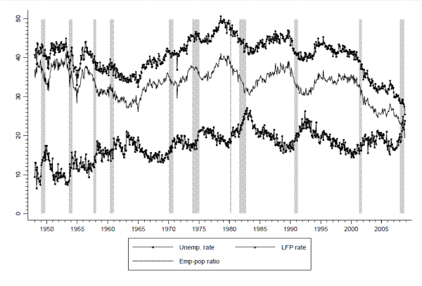
Figure 2: Trends in employment-population ratio for youth and adult males, 1948-2008 (seasonally adjusted)

Note: estimates are published statistics from the Bureau of Labor Statistics. Graph plots the seasonally-adjusted employment-population ratio for all youth age 16-17 and adult males older than 25. Shaded regions indicate recessionary periods as determined by the NBER.

Figure 2 Data

Figure 3: Share of natives in top immigrant industries and occupations, by age and sex

Note: Panel A plots the share of each age group employed in the top twenty most common occupations for immigrants with a high school degree or less in 1980, conditional on employment. Panel B plots a similar share for the twenty most common industries among low-skilled immigrants. Panel C plots a similar share for the seventy-five most common industry-occupation pairs among less-educated immigrants.

Figure 3 Data

Figure 4: Impact of less educated immigration on employment, by age and sex

Note: Plots represent 2SLS estimaqtes of immigration effects from regressions changes in employment measures (by age) on changes in the log number of less-educated adult immigrants (analogous to regression results presented in table 4). Estimates are smoothed across ages using local linear regression with a bandwidth of .3.

Figure 4 Data

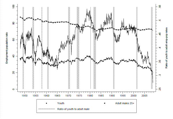
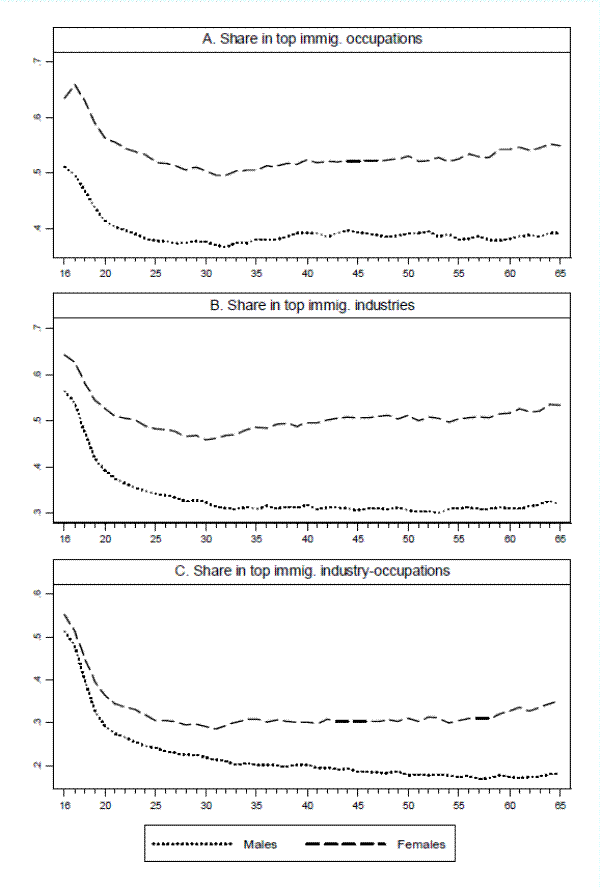
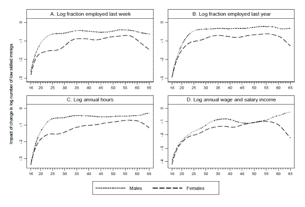
Data Appendix

Census and ACS data come from the Integrated Public Use Microdata Series (IPUMS) public use extracts (Ruggles et al. 2009). 1970 extracts are from the 1% form 1 state and metro samples. 1980, 1990, and 2000 extracts are from the 5% sample. Immigrants are defined as individuals who report being born out of the country and either non-citizens or naturalized citizens. Less-educated individuals are defined as those who report having at most a high school degree (no college). Labor market variables are calculated after first dropping those who report residing in group quarters. An individual is coded as working in the previous week if they report their employment status as at work or having a job but not working. An individual is coded as working in the previous year if he or she reports positive weeks worked in the previous year. Weeks worked in 1970 is reported in intervals rather than the exact number of weeks. For those with positive weeks worked in 1970, I assign the average weeks worked for the interval (conditional on age and gender) as calculated with 1980 data. Weekly wages are calculated as annual wage and salary income divided by weeks worked. Annual hours worked are calculated as weeks worked in the previous year multiplied by usual weekly hours.

Appendix Table 1A : Summary statistics for employment outcomes for
Native teens (age 16 and 17), male

	Fract. employed last week (1)	Fract. with pos. annual weeks worked (2)	Average weeks worked for workers (3)	Average weekly wage (4)	Average annual hours worked (5)	Average annual wage and salary income (6)
1970	0.32	0.52	10.6	$287.8	162.5	$2,440
1980	0.33	0.51	11.7	$228.2	276.6	$2,175
1990	0.32	0.51	11.3	$186.1	241.4	$1,709
2000	0.31	0.45	10.2	$209.1	212.8	$1,744
2005	0.24	0.41	8.0	$172.1	156.7	$1,136

Notes: 1970, 1980, 1990, and 2000 data come from the Decennial Census (IPUMS). 2005 data come from the American Community Survey (IPUMS). Average weeks worked and annual hours worked are averaged over all individuals (including zeros). Average weekly wage is averaged only over those with positive wages. Average annual wage and salary income is averaged over everyone (including zeros). Weekly wage and annual wage and salary income are reported in 2009 dollars.

Appendix Table 1B : Summary statistics for employment outcomes for
Native teens (age 16 and 17), female

	Fract. employed last week (1)	Fract. with pos. annual weeks worked (2)	Average weeks worked for workers (3)	Average weekly wage (4)	Average annual hours worked (5)	Average annual wage and salary income (6)
1970	0.20	0.33	6.0	$251.8	75.8	$1,257
1980	0.29	0.43	9.4	$191.2	195.8	$1,484
1990	0.32	0.48	10.8	$161.8	210.5	$1,444
2000	0.33	0.45	10.5	$189.1	201.4	$1,571
2005	0.28	0.42	9.0	$144.9	161.0	$1,131

Notes: 1970, 1980, 1990, and 2000 data come from the Decennial Census (IPUMS). 2005 data come from the American Community Survey (IPUMS). Average weeks worked and annual hours worked are averaged over all individuals (including zeros). Average weekly wage is averaged only over those with positive wages. Average annual wage and salary income is averaged over everyone (including zeros). Weekly wage and annual wage and salary income are reported in 2009 dollars.

Appendix Table 1C : Summary statistics for employment outcomes for
Native adults (age 22-64), male

	Fract. employed last week (1)	Fract. with pos. annual weeks worked (2)	Average weeks worked for workers (3)	Average weekly wage (4)	Average annual hours worked (5)	Average annual wage and salary income (6)
1970	0.87	0.94	45.3	$877.0	1805.7	$36,274
1980	0.80	0.88	41.4	$863.5	1789.5	$31,965
1990	0.77	0.86	39.5	$848.8	1720.2	$29,730
2000	0.74	0.83	39.1	$891.1	1716.1	$30,291
2005	0.72	0.83	38.0	$868.0	1658.0	$28,893

Notes: 1970, 1980, 1990, and 2000 data come from the Decennial Census (IPUMS). 2005 data come from the American Community Survey (IPUMS). Average weeks worked and annual hours worked are averaged over all individuals (including zeros). Average weekly wage is averaged only over those with positive wages. Average annual wage and salary income is averaged over everyone (including zeros). Weekly wage and annual wage and salary income are reported in 2009 dollars.

Appendix Table 1D: Summary statistics for employment outcomes for
Native adults (age 22-64), female

	Fract. employed last week (1)	Fract. with pos. annual weeks worked (2)	Average weeks worked for workers (3)	Average weekly wage (4)	Average annual hours worked (5)	Average annual wage and salary income (6)
1970	0.44	0.54	21.5	$470.3	670.1	$9,707
1980	0.51	0.59	24.8	$456.4	909.8	$10,837
1990	0.57	0.66	28.3	$499.6	1053.7	$13,210
2000	0.58	0.68	30.2	$579.3	1142.9	$15,702
2005	0.58	0.68	30.2	$565.5	1131.6	$15,656

Notes: 1970, 1980, 1990, and 2000 data come from the Decennial Census (IPUMS). 2005 data come from the American Community Survey (IPUMS). Average weeks worked and annual hours worked are averaged over all individuals (including zeros). Average weekly wage is averaged only over those with positive wages. Average annual wage and salary income is averaged over everyone (including zeros). Weekly wage and annual wage and salary income are reported in 2009 dollars.

Appendix Table 2 : Summary statistics for immigration measures

		Average change in log number of less-educated adult immigrants (in log points) (1)	Average percentage point change in immigrant share of less-educated adult population (2)	Average change in total log number adult immigrants (in log points) (3)	Average percentage point change in immigrant share of total adult population (4)
	1970 to 1980	-44.9	1.7	-31.4	1.9
	1980 to 1990	14.1	4.7	33.7	4.2
	1990 to 2000	64.5	7.1	62.2	5.7
	2000 to 2005	15.7	1.9	18.9	1.6

Notes: 1970, 1980, 1990, and 2000 data come from the Decennial Census (IPUMS). 2005 data come from the American Community Survey (IPUMS). Less educated individuals are defined as those with a high school degree or less. Adults are individuals age 22 to 64 at the time of the Census or ACS survey. Averages are weighted by the number of people (16-64) in the commuting zone in the later year.

Footnotes

1. Revised from earlier version (January 2008). The views in this paper are solely the responsibility of the author, and should not be interpreted as reflecting the views of the Board of Governors of the Federal Reserve System, or any other persons associated with the Federal Reserve System. Thanks to the following individuals for thoughtful comments: David Autor, Josh Angrist, Neil Bhutta, Tal Gross, and seminar participants from MIT, the Federal Reserve Board of Governors, the 2008 annual meeting for the Society of Labor Economics, and numerous other seminars. I especially thank David Autor and David Dorn for providing assistance with commuting zone classification. All errors are my own. Return to Text

2. Estimates of the national impact of immigration on native employment tend to be negative and larger in magnitude. See Borjas (2003) and Borjas (2006). Return to Text

3. One exception is Sum, Harrington, and Kathiwada (2006), which uses 2003 American Community Survey data to estimate the cross-state relationship between the relative size of immigrant inflows into a state and employment rates for young natives (age 16-24). They find that a 1 percentage point increase in a state's population due to immigration is associated with a 1.2 percentage point reduction in the employment rate for young adults. Aaronson, Park and Sullivan (2006) consider immigration as an alternative explanation for recent declines in youth employment by extending the Mariel boatlift analysis from Card (1990) to the youth labor market. They find that teen employment rates in Miami increased more than they did in comparable cities after the influx of low-skilled Cuban immigrants, suggesting against large and negative employment effects for teens. Although this evidence is suggestive, it comes from a single case study, and there may be significant heterogeneity in immigration effects across cities and decades. Return to Text

4. For reference, the size of the less-educated immigrant population increased by more than 200 percent on average across commuting zones between 1980 and 2005. Return to Text

5. The minimum wage introduces one additional complexity. If wages are low enough so that the minimum wage is binding for teens and immigrants, then an increase in immigration may affect youth employment more strongly because their wages are constrained from falling further. This result also assumes that, for a given wage, employers prefer adult immigrants to youth--which might be true because adult immigrants tend to have more work experience, might have stronger work ethic, or may accept greater flexibility in their work schedules (because they can work during the school day and because there are fewer laws constraining their hours of work). Consistent with this, it is well-documented that teens are the first ones fired in a recession: employers seem to utilize teen labor to meet temporary demand shocks, and adjust to negative shocks by firing youth first (for instance, see Jaimovich, Pruitt and Siu 2009). Return to Text

6. For instance, if an individual reports living in a PUMA that crosses two commuting zones, and exactly half of the PUMA population lives in each commuting zone, then the individual is recorded as living in each commuting zone, but his or her sample weight is halved. Return to Text

7. Including native stocks is problematic if the number of natives in an area is also responsive to changes in immigration. In the next section, I demonstrate that this does not seem to be true empirically. Return to Text

8. I weight by , where is the sum of census weights for the age-gender-area-year cell. This formula is derived from calculations for the variance in a first-differenced outcome variable, and assumes that each cell mean is measured with error, that the variance in measurement error within a year is proportional to its weight, and that measurement error is independent across years. Return to Text

9. I divide originating countries into 16 groups based on geographic and cultural similarities. Return to Text

10. This may be violated if, for example, certain industries are more likely to employ immigrants of a particular ethnicity, and these industries experienced a national (decade-long) shock; then, areas with high concentrations of this ethnicity would have greater declines in native employment for reasons other than the increased number of immigrants. Since this analysis is limited to less-educated immigrants, the skill set of the immigrant population should be homogenous enough so that this is not a concern. Return to Text

11. Because I am unable to construct commuting-zone area measures for 1960, I use the contemporaneous - rather than the lagged - ethnic composition to form the index in 1970. Return to Text

12. I divide by , where the first term is the median ratio of immigrants to natives across all areas in 1970 multiplied by the size of the native stock in 1970 in area (a plausibly exogenous measure of the number of immigrants in 1970), and the second term is the predicted increase in immigration from 1970 to from (4). Return to Text

13. Teens constitute a single age group. Adults age 24-64 are divided into groups with five year age intervals. Return to Text

14. For some cells, no individuals report being employed. For these, I record the employment rate as zero, the log employment rate as log(1/n) where n is the cell size, and the log of annual hours worked as zero. Return to Text

15. As controls, I include year fixed effects, the change in the log number of less-educated native adults, the share of natives without a high school degree, the share of natives with a college degree, the share of natives that are black, and the share of natives who are male (the shares are all measured in time . One might worry that the change in the number of natives is endogenous (in particular, that natives leave when immigrants enter, biasing employment effects toward zero). However, 2SLS regressions of the change in the log number of less-educated natives on the log number of less-educated immigrants suggest that, if anything, the number of natives increase in cities that experience a greater increase in immigration (the regression coefficient is 0.06 and the clustered standard error is 0.03). Return to Text

16. This is equivalent to dividing the immigration effect in column 3 by that in column 2 (or column 10 by column 9), but estimating separate labor supply equations instead allows direct estimation of the associated standard errors. Return to Text

17. Another potential explanation is that the minimum wage tends to be more binding for youth than for adults. If: 1) the minimum wage constrains youth wages from falling in response to immigration, 2) both immigrants and youth tend to earn the minimum wage, and 3) employers would prefer hiring less-educated adult immigrants to native youth for a given wage, then immigration may affect youth employment without having an observable impact on their wage. If this were true, then the wage effect of immigration would be larger in states for which the minimum wage was more binding (for example, in areas where a higher fraction of teens were earning wages around the minimum). Empirically, this appears to be the case: regressions of (3) that include the change in immigration interacted with measures of the bindingness of the minimum wage in suggest that wage effects are greater in more binding states (results available upon request). If this differential is due to the minimum wage and not some other inherent difference between states that is correlated with the bindingness of the minimum wage, then the impact of immigration on employment should be smaller in high wage states, since wages are more able adjust. However, the reverse appears to be true, suggesting that the minimum wage may not be an explanation for small wage effects. Return to Text

18. See Tyler (2003), DeSimone (2006) and Oettinger (1999) for estimates of employment effects on grades and test scores (the first finds negative effects, while the latter two find modest positive effects for low levels of school-year employment and negative effects for more substantial employment). See also Ruhm (1997), which finds positive effects of youth employment on future earnings, and Hotz, Xu, Tienda, and Ahituv (2002) which argues that returns appear insignificant after properly controlling for unobserved heterogeneity and sample selection. Return to Text

19. An example may help illustrate the setup. Consider the group of individuals who were 25 to 28 and lived in New York State at the time of the Census, and who were born in Florida. This regression relates log annual earnings for this group in 1980, 1990 and 2000 to log annual hours worked for 16 and 17 year olds in Florida in 1970, 1980, and 1990. Return to Text

^♣ This version is optimized for use by screen readers. Descriptions for all mathematical expressions are provided in LaTex format. A printable pdf version is available. Return to Text

Home | Economic Research and Data | Accessibility | Contact us
Last update: January 11, 2010