Exports, Borders, Distance, and Plant Size
Keywords: Border effect, plant size, exports
Abstract:
The fact that large manufacturing plants export relatively more than small plants has been at the foundation of much work in the international trade literature. We examine this fact using Census micro data on plant shipments from the Commodity Flow Survey. We show the fact is not entirely an international trade phenomenon; part of it can be accounted for by the effect of distance, distinct from any border effect. Export destinations tend to be further than domestic destinations, and large plants tend to ship further distances even to domestic locations, as compared with small plants. We develop an extension of the Melitz (2003) model and use it to set up an analysis with model interpretations of ratios between large plant and small plant shipments that can be calculated with the data. We obtain a decomposition of the overall ratio into a term that varies with distance, holding fixed the border, and a term that varies with the border, holding fixed the distance. The distance term accounts for more than half of the overall difference.
1 Introduction
Large manufacturing plants export relatively more than small plants (Bernard and Jensen (1995)). This fact has been at the foundation of a large and influential literature that analyzes international trade at the plant level, including Melitz (2003); Eaton and Kortum (2002); and Bernard, Eaton, Jensen, and Kortum (2003). The literature focuses on how large plants overcome impediments to international trade, such as investing in foreign distribution channels as emphasized in Melitz (2003).
The starting point of this paper is the observation that the plant-size export relationship may not be entirely an international trade phenomenon. It can also be accounted for by the effect of distance, apart from any border effect. Large plants may tend to ship further distances than small plants, even for internal flows to domestic destinations. Since foreign destinations typically are further than domestic destinations, any advantage large plants might have in long distance shipping would make them more likely to export, even if large plants had no particular advantage in surmounting international trade borders.
This paper presents a straightforward generalization of the Melitz (2003) model in which plants make one investment to overcome distance barriers and a second investment to overcome border barriers. We show how the plant-size/export relationship can be decomposed into two terms. The first term, the size-distance ratio, depends on distance shipped, holding fixed the border. The second term, the size-border ratio, varies the border, holding distance fixed. These ratios--which can be calculated directly from the data--have a theoretical interpretation in the model in terms of barriers to distance and barriers at the border.
Our empirical analysis uses the Commodity Flow Survey (CFS), a micro data set at the U.S. Census Bureau on shipments originating at U.S. manufacturing plants. This data resource is unique in the comprehensive way that it tracks originations and destinations both for domestic shipments and for exports. We use these data to decompose the plant-size/export relationship into its distance and border components. We find that the distance component is more than half of the total overall relationship. The finding is robust over various alternative ways we cut the data. In short, we find that not only are large plants more likely to export, they are also more likely to ship long distances within the United States, compared with small plants. The estimated relationship between plant size and distance shipped internally within the United States is large enough to account for more than half of the plant-size/export relationship, in a sense that we make precise.
It is natural to expect that the same forces that might determine whether or not a plant in Michigan is selling to export markets like Mexico, would also determine whether or not the plant is shipping long distance within the United Statesto places like California or Maine. By the same logic that plants might need to make investments in foreign distribution channels, they also might need to make investments in domestic distribution channels as well. Fully understanding this mechanism is useful if we want to understand trade flows and how they might change with changes in policy. For example, it may not make much difference for a government trade agency to assist a Michigan plant with Spanish-language paperwork needed for exports to Mexico, if the Michigan plant is unable to overcome the internal distance barrier to shipping goods to Texas.
The analysis is closely related to the border study literature initiated by McCallum (1995). (See Anderson and van Wincoop (2003) for a more recent treatment and Anderson and van Wincoop (2004) for a survey.) Our paper follows this literature in the way it disaggregates the geography of a country and distinguishes between internal trade flows within a country and external trade flows across borders. In the literature, to determine the border effect, trade between two locations within the same country at a given distance is compared with trade between locations separated by a border, but otherwise the same distance. Our paper is distinct from this earlier literature because rather than look at the level of trade by distance and border, our paper looks at the changes in trade by distance and border, comparing them with changes in plant size. The fact that we are differencing by plant size means we don't have to get into details about demand (e.g., gravity) that are front and center in the earlier border literature. In what we do, demand differences out. In summary, our paper takes from the border literature its disaggregated geography and uses it to analyze the plant-size/export relationship, which plays a central role in plant-level trade literature. We thereby connect two important literatures.
While we frame the theoretical discussion in terms of an extension of the Melitz (2003) model of investments in distribution channels, as this theory is well known and tractable for our purposes, our empirical results are equally applicable for the theory we develop in Holmes and Stevens (2010). That paper argues that even within narrowly defined industries, small plants tend to perform retail-like functions that are difficult to trade (e.g., custom work), compared with large plants in the same industry. This factor not only explains why a small Michigan plant would be unlikely to do business in Mexico, it also explains why the small Michigan plant would be unlikely to do business in California. Our findings in Holmes and Stevens (2002, 2010) that small plants tend to be geographically diffuse and follow the distribution of population, while large plants tend to be geographically concentrated, is consistent with the shipment distance findings reported here. As the small plants follow the distribution of population, they can meet demand by serving local customers, just like retail stores do. As the large plants may be concentrated in just a few locations, goods must be shipped to distant locations that have no source of local supply.
We mention a few other related papers. Hummels and Hillberry (2003, 2008) were the first to use the micro data version of the CFS. They used these data to conduct a border analysis analogous to what McCallum did for the U.S.-Canada border, only Hummels and Hillberry looked at the effect of state borders within the United States. Our paper shares a common feature with Bernard, Jensen, and Schott (2009) in being a transaction-level analysis of shipments linked to characteristics of the shipment source. (See also Bernard, Jensen, Redding, and Schott (2007).) Their data are based on the administrative records of all international trade transactions that go through customs. There is no analog of a customs house tracking internal shipments across states. The CFS that we use here is a unique resource, as it has both exports and internal shipments as part of one data source.
The rest of the paper proceeds as follows. Section 2 presents the extension of Melitz (2003) in which the decomposition between the distance ratio and the border ratio is developed. Second 3 describes the data. Section 4 presents the empirical results. Section 5 briefly concludes.
2 Theory
We present a generalization of the Melitz (2003) model in which plants make shipments of varying distances both to domestic locations and foreign locations. As in Melitz, plants can make investments to lower the marginal cost of distribution. What is different here is that these investments can be made both for domestic shipments as well as foreign shipments.
We use the model to develop ratios and then take ratios of ratios, setting up the main empirical analysis of the paper. The ratio analysis is useful, because various model terms cancel out in the ratios and enable us to isolate empirical magnitudes that are relevant for sorting out the relative importance of the size/distance relationship and the size/border relationship.
2.1 Description of the Model
There is a discrete set of locations, indexed by ![]() , some of which are domestic and others of which are foreign. We start by describing the environment for a particular plant located at
a particular domestic location and later add more notation to take account of other plants. The demand for the plant's product at a location
, some of which are domestic and others of which are foreign. We start by describing the environment for a particular plant located at
a particular domestic location and later add more notation to take account of other plants. The demand for the plant's product at a location ![]() (which may be different from where the plant
is located) depends on the local price
(which may be different from where the plant
is located) depends on the local price ![]() the plant sets to the location, as well as the population
the plant sets to the location, as well as the population ![]() at the location, and takes the following functional form
at the location, and takes the following functional form
The parameter
Now, consider a particular location that is a distance ![]() miles away from the plant. For simplicity, we temporarily drop the subscript
miles away from the plant. For simplicity, we temporarily drop the subscript ![]() . In selling to this location, the plant faces a distance friction. In addition, if the selling location is in the foreign country, the plant faces a border friction.
. In selling to this location, the plant faces a distance friction. In addition, if the selling location is in the foreign country, the plant faces a border friction.
The extent of the distance friction is summarized by a variable ![]() , which has the standard "iceberg transportation cost"form, so that if the plant intends to deliver one unit to the
location, it has to ship
, which has the standard "iceberg transportation cost"form, so that if the plant intends to deliver one unit to the
location, it has to ship ![]() . We allow the transportation cost
. We allow the transportation cost ![]() to be altered
by the plant making an investment
to be altered
by the plant making an investment ![]() to improve its distribution network to the particular market. In particular, suppose the required investment to attain transportation cost
to improve its distribution network to the particular market. In particular, suppose the required investment to attain transportation cost ![]() depends on the size
depends on the size ![]() of the market as well as the mileage
of the market as well as the mileage ![]() to the market in the following way
to the market in the following way
where
and for
 ,
,  ,
, 
and there exists a lower bound
while
Assumption (3) just says that when the mileage distance is zero, no investment must be made to attain the zero transportation cost limit of
Analogous to the way the distance friction is modeled, the border friction is summarized by a variable ![]() , which also has the iceberg cost format. Holding distance
, which also has the iceberg cost format. Holding distance ![]() fixed, to get one unit over the border, the plant must ship
fixed, to get one unit over the border, the plant must ship ![]() units. Analogous to the
way
units. Analogous to the
way ![]() can be altered, we allow the plant to alter
can be altered, we allow the plant to alter ![]() by making investments. Suppose
there is an ad valorem tariff
by making investments. Suppose
there is an ad valorem tariff ![]() . The plant chooses a level of
. The plant chooses a level of
![]() . (We keep
. (We keep ![]() bounded above
bounded above ![]() because the tariff must be paid, regardless of the investment.) The extent that
because the tariff must be paid, regardless of the investment.) The extent that ![]() is above the tariff reflects other
barriers at the border, such as language or dealing with the complexities of shipping to the foreign country. The plant can lower
is above the tariff reflects other
barriers at the border, such as language or dealing with the complexities of shipping to the foreign country. The plant can lower ![]() by making an investment. Let
by making an investment. Let ![]() be the investment in reducing border costs and assume it takes the form
be the investment in reducing border costs and assume it takes the form
 ,
,and that there is a
but
Assumption (9) says it costs resources to lower the friction. Assumptions (10) and (11) are an Inada condition ensuring an interior choice of
2.2 Optimal Firm Behavior
Given the distance and border frictions ![]() and
and ![]() , the plant has constant marginal
cost of
, the plant has constant marginal
cost of ![]() to deliver one unit to a domestic location and
to deliver one unit to a domestic location and
![]() for a foreign location. (Again,
for a foreign location. (Again, ![]() is the constant marginal cost of
production at the plant's location.) Since demand is constant elasticity, the profit maximizing price if the location is domestic equals a markup over costs,
is the constant marginal cost of
production at the plant's location.) Since demand is constant elasticity, the profit maximizing price if the location is domestic equals a markup over costs,
and if foreign
Next, consider the plant's choice of ![]() and
and ![]() . For a domestic location, the plant
chooses
. For a domestic location, the plant
chooses ![]() to solve
to solve
 ,
,for
The second line follows from straightforward substitution of (12) and (1) into the above. The third line collects the various multiplicative parameters that affect sales. Observe that the population
Analogously, for a foreign destination, ![]() and
and ![]() are chosen to solve,
are chosen to solve,
![\displaystyle N\left\{ \max_{a\geq 1\text{, }b\geq 1+\tau }\theta \left[ ab\right] ^{-\left( \eta -1\right) }-f(a,m)-g(b)\right\} \text{.}](img58.gif)
This structure generalizes the familiar Melitz (2003) environment in a straightforward way. In Melitz, rather than a continuous relationship between the friction ![]() and investment spending
and investment spending
![]() , there is a discontinuous relationship. In particular, suppose the investment cost
, there is a discontinuous relationship. In particular, suppose the investment cost ![]() takes the following form:
takes the following form:
| 0, for |
For this special case of the
Making the relationship between the frictions and investments continuous, and adding both a distance friction as well as a border friction, leads to the same qualitative insights as in Melitz.1 Let
![]() ,
,
![]() , and
, and
![]() denote the solutions to problems (14) and (16) as a function of plant productivity
denote the solutions to problems (14) and (16) as a function of plant productivity ![]() and distance to market
and distance to market ![]() . The following result provides our key comparative statics results about the solution
to the plant's problem.
. The following result provides our key comparative statics results about the solution
to the plant's problem.
Proposition 1. Assume (3) through (11) hold. Then (i) the optimal choice of the frictions
![]() ,
,
![]() ,
,
![]() , all decrease in
, all decrease in ![]() and increase in
and increase in ![]() , (ii) the inequality
, (ii) the inequality
![]() holds, and(iii) as productivity gets arbitrarily large, the frictions go to the lower bounds,
holds, and(iii) as productivity gets arbitrarily large, the frictions go to the lower bounds,
![]()
![]()
![]() ,
,
![]()
![]()
![]() , and
, and
![]() .
.
Proof of (i). We prove the result for the case of a foreign destination; the case of a domestic destination is similar. Let
![]() denote the profit per capita in a foreign market given choices
denote the profit per capita in a foreign market given choices ![]() and
and ![]() , and given productivity
, and given productivity ![]() and market distance
and market distance
![]() . (This is the term in braces in the second line of (16).) Treating
. (This is the term in braces in the second line of (16).) Treating ![]() and
and ![]() as the choice variables, the first-order necessary conditions are
as the choice variables, the first-order necessary conditions are
 |
 |
||
 |
 . . |
Taking cross partials yields
 |
|||
 |
|||
 |
|||
 |
 |
||
 |
0. | ||
 |
0 |
Hence, the objective
Proof of (ii). Observe the domestic market is just like the foreign market except the equivalent border term for the domestic market ![]() without paying any
costs. Next, note assumption (10) implies
without paying any
costs. Next, note assumption (10) implies
![]() . The result then follows from the supermodularity of
. The result then follows from the supermodularity of ![]() in
in ![]() and
and ![]() .
.
Proof of (iii). This follows from the FONC and the Inada assumptions (7), (8),(10), and (11). Q.E.D.
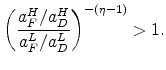
The logic underlying Proposition 1 is exactly the scale economy logic in Melitz. The larger market of a more productive plant will make it more willing to pay fixed cost to lower marginal costs both with regards to the distance friction as well as the border friction. Consider next a given plant selling to two markets the same mileage distance, but one is domestic and the other is foreign. Given the border friction in the latter market, there is greater sales volume in the former market. Hence, a plant will be more likely to invest in reducing the distance friction in a domestic market of a given mileage distance than a foreign market.
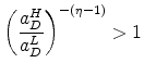
For what we will do below, it is useful to define the following ratio as a function of ![]() and
and ![]()
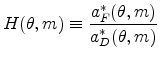 .
.From Proposition 1(ii),
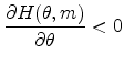 , for
, for 2.3 Ratios
Later in this paper, we will be working with revenue data by plant size class. In this subsection, we show how we can take ratios of revenues across different plant size groupings in such a way that various model parameters cancel out, providing us with useful statistics that can be connected to the model and that provide insight.
Our first step is to derive formulas for revenues. The revenue measures will be net of the transportation cost and border frictions ![]() and
and ![]() , as this corresponds to what we have in the data. Let
, as this corresponds to what we have in the data. Let
![]() be net sales revenue for a plant of productivity
be net sales revenue for a plant of productivity ![]() summed
over all domestic locations
summed
over all domestic locations ![]() miles away. To derive the formula, let
miles away. To derive the formula, let ![]() be
the total population summed over all domestic markets at distance
be
the total population summed over all domestic markets at distance ![]() . Given
. Given ![]() ,
sales per capita in each distance
,
sales per capita in each distance ![]() domestic market is the same in each market. Using formula (12) for price and plugging this into demand (1), it is
straightforward to derive that domestic market per capita revenue given
domestic market is the same in each market. Using formula (12) for price and plugging this into demand (1), it is
straightforward to derive that domestic market per capita revenue given ![]() equals
equals
![]() . Taking into account population, domestic revenue at distance
. Taking into account population, domestic revenue at distance ![]() for a type
for a type ![]() firm equals
firm equals
Note that for simplicity, we leave implicit the dependence of
Now, we define the key ratios. We will refer to domestic locations that are ![]() miles away as "near"locations and examine sales relative to this. Define the Export-Near Ratio to be the ratio of foreign sales at distance
miles away as "near"locations and examine sales relative to this. Define the Export-Near Ratio to be the ratio of foreign sales at distance ![]() relative to domestic near sales. This ratio can be decomposed into a product of the Distance Ratio and the Border Ratio as follows:
relative to domestic near sales. This ratio can be decomposed into a product of the Distance Ratio and the Border Ratio as follows:

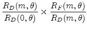
The Distance Ratio takes domestic sales at distance
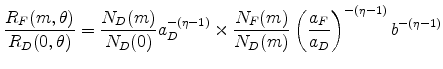 ,
,Next, we compare plants of different ![]() and take ratios of ratios. Let
and take ratios of ratios. Let
![]() be high and low productivity levels and define the Size Export-Near Ratio by taking the ratio of the far-near ratios for the two
productivity types, putting the high type in the numerator. Analogous to (21), it can be decomposed into a product of two terms,
be high and low productivity levels and define the Size Export-Near Ratio by taking the ratio of the far-near ratios for the two
productivity types, putting the high type in the numerator. Analogous to (21), it can be decomposed into a product of two terms,
| Size Export-Near Ratio |  |
||
| Size-Distance Ratio |
for
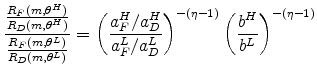
From Proposition 1,
It is useful to discuss what these ratios look like in two extreme cases. The first extreme case is the Border-Investment-Only Case. Here, there are no internal distance frictions within the domestic country
![]() nor within the foreign country
nor within the foreign country ![]() , while there is a friction
at the border. Thus, there is frictionless trade to ship internally to the border, a transactions cost to cross the border, then again frictionless trade within the foreign country. Typical analyses of exports are implicitly working with this special case. For this extreme case, the ratios reduce
to,
, while there is a friction
at the border. Thus, there is frictionless trade to ship internally to the border, a transactions cost to cross the border, then again frictionless trade within the foreign country. Typical analyses of exports are implicitly working with this special case. For this extreme case, the ratios reduce
to,
| Size-Distance Ratio | |||
| Size-Border Ratio | 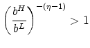 |
so
Thus, differences across plant size in propensity to export are driven entirely by differences at the border.
An opposite extreme case is the Distance-Investment-Only Case. This case allows for there to be a friction at the border (e.g., a tariff or physical processing cost, or something else), but it is not possible to make investments to reduce it. So all firms from all
size classes have the same border friction
![]() , which we assume is greater than one
, which we assume is greater than one
![]() .In this case, the component ratios are
.In this case, the component ratios are
So even in this extreme case where there are no border investments, the Size-Border Ratio exceeds one.
In the analysis below, we will calculate the Size Export-Near Ratio and its multiplicative decomposition into the Size-Distance Ratio and the Size-Border Ratio.
3 The Data
The Census Bureau's Commodity Flow Survey(CFS), conducted in cooperation with the U.S. Department of Transportation, is a survey of the shipments originating in manufacturing, wholesale, and mining establishments. At one extreme, a shipment can include a rail car (or group of rail cars) or a container or a truckload of a particular commodity. At another extreme, a shipment can include a half pound medical device sent overnight via Federal Express. The sample is constructed as follows. First, the Census Bureau selects a sample of plants to be in the survey, using a particular set of sampling weights. Second, the plants in the sample in turn select a random sample of their shipments over the course of a particular week in each quarter of the year. For each shipment in the sample, the origin and destination is reported, as well as the weight (in pounds), the value, the modes of transport, and some additional information.
The CFS is taken every five years in the same years that the Census of Manufacturing (CM) is taken. We use the 1997 CFS. It consists of more than 5 million shipments sampled from 64,000 different plants. We restrict attention to the manufacturing sector and match 2.7 million CFS shipment records to 30,148 manufacturing establishments in the 1997 CM.
Table 1 presents the basic facts about plant size and distance shipped in the 1997 Manufacturing CFS. The shipment shares are calculated using the dollar value of the shipment and the sampling weights. The distance measure is the "great circle"or "as the crow flies"distance between locations.2 The first row uses all the plants in the data. Over the entire sample, the dollar-weighted shipment share going to export destinations equals 0.103. For domestic destinations, the shares are broken down by distance-shipped categories. The shares of shipments going Near (less than 100 miles), Mid-Distance (between 100 and 500 miles), and Far (more than 500 miles),equal 0.261, 0.288, and 0.348, respectively.
The remaining rows of table 1 break the sample up by plant employment size categories. The first thing to note about these shares is the well-known pattern that export shares increase substantially with plant size. (See Bernard and Jensen (1995).) Going from the smallest plant size category to the largest, the export share increases by a factor of more than three, from 0.040 to 0.138.
The second thing to note is that a similar pattern is at work with internal shipments within the United States. Thispattern is the key fact that will be driving our main results in the ratio analysis. The share shipped to far domestic locations increases substantially withplant size. The smallest plant size category sends only a share of 0.194 to far destinations. The largest plant size category ships to this distance at twice this rate (a share equal to 0.338). The last column reports the mean mileage of distance shipped by employment size category. (For exports, distance shipped only includes the U.S. portion of the shipment's journey, as we will further explain.) There is a clear pattern that mean mileage of distance shipped increases with plant size, equaling 327 miles in the smallest category and rising to 589 miles for the largest.
The analysis in the theory holds distance shipped fixed when comparing internal shipments and exports. So we need account for the shipment distances of exports. Note that while exports typically go further distances than domestic shipments, it certainly can happen that an export goes a shorter way than a domestic shipment. For example, Windsor, Ontario, lies right across the Canadian border from Detroit, Michigan. An export from Detroit to Windsor might be only 5 miles. In contrast, a shipment from the East Coast to the West Coast of the United States will travel 3,000 miles.
Each shipment in the CFS has a location code both for origin and destination and a mileage variable is reported between the origin and the destination. However, for exports, the destination code that is given is for the port of exit in the United States. Thus, the reported mileage is not the full mileage to the ultimate destination, rather the mileage for the internal portion of the journey up to the point of exit. In the 1997 CFS, there is a text field in the data that specifies the destination country. We process this text field to classify exports into three destinations: Canada, Mexico, and "Rest of the World." 3
We set up the distance structure of analysis as follows. We group distances of 500 miles and above as being the same and call these distances far. When we look at exports to Canada, we use only observations for plants in the United States that are located at least 500 miles from the Canadian border. Hence, all of these exports must be going at least 500 miles. Analogously, when we look at exports to Mexico, we use only observations for plants that are at least 500 miles from the Mexican border. So all of these exports are necessarily going further than 500 miles. Finally, exports to the rest of the world besides Mexico and Canada go more than 500 miles from all locations in the contiguous United States, so we use all of the plants in the data for these exports.
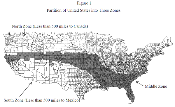
Figure 1 divides the contiguous United States into three zones, based on distance to the Canadian and Mexican borders. We use counties as the underlying geographic unit. The North Zone are those counties located within 500 miles of the Canadian border.4 The South Zone consists of all counties within 500 miles of the Mexican border. The Middle Zone lies in between. The Middle Zone is of particular interest. For any plant located in this zone, all exports necessarily travel more than 500 miles. For plants in the South Zone, if we throw out exports to Mexico, then all the remaining exports necessarily travel more than 500 miles. Analogously, we have this effect for plants in the North Zone when we throw out exports to Canada.
Table 2 provides some summary statistics by the geographic zones. The North Zone contains more than half of the shipment observations in the sample and more than half of the manufacturing plants in the underlying universe of plants. We note that with our 500 mile cutoff distance to Canada, we are using a broad definition of "North"that groups all of Virginia and most of North Carolina and Tennessee into the North Zone. The Middle and South Zones are similar, in accounting for roughly one-fifth of the manufacturing plants and employment in the underlying universe, and roughly one-fifth of the sample shipments. Average plant employment size is 48.7 in the Middle Zone, which is similar to the average in the North Zone and to the overall mean. Plants are somewhat smaller, on average, in the South Zone.
We note that we don't use a higher cutoff to define far shipments, as this would cause us to lose many observations. For example, if we set the cutoff to 1,000 miles and require a location to be more than 1,000 miles from both the Canadian and the Mexican border, then only six counties at the southeastern tip of Florida would qualify.
4.1 Benchmark Results
As explained in the previous section, we group shipment distances further than 500 miles together as being equivalent, a far shipment. We will also group shipment distances of less than 100 miles together and call these near shipments. In
the ratio analysis, we will treat near shipments as corresponding to the mileage ![]() case in the theory.
case in the theory.
Table 3 presents shipment shares by destination category and plant sizefor plants in different geographic zones. For example, Panel A reports the shares for plants in the South Zone (i.e., plants within 500 miles of Mexico). Each panel reports the shipment shares for near and far domestic locations and far foreign locations. To ensure that all the foreign shipments go at least 500 miles, we make certain deletions regarding exports. For Panel A, we delete all exports to Mexico, so the statistic reported in the column labeled "Foreign Far"is the share of all shipments that are exports to countries besides Mexico. That is, all exports necessarily travel more than 500 miles. We don't need to make any deletions for the Middle Zone in Panel B. For the North Zone plants in Panel C, we delete exports to Canada. Finally, the last panel uses all plants across the three zones. For this, we delete all exports to Canada and Mexico for all plants, even those in the Middle Zone, to be consistent.
Note that across all four samples of plants, the domestic near share falls sharply with plant size, while the domestic and foreign far shares both increase sharply with plant size.
Table 4 uses the shares in the various samples of table 3 to construct the ratios defined in the theory for each sample. The Export-Near Ratio is calculated by taking, for each size class, the ratio of foreign far shipments to domestic near shipments The Distance Ratio is domestic far sales divided by domestic near sales. The Border Ratio is the ratio of foreign far to domestic far. The latter holds constant distance, because all shipments in the numerator and denominator exceed 500 miles (and because we are treating distances above 500 miles as the same).
The last three columns contain the ratios across plant size categories of the ratios in the previous three columns. For each row, we are putting the largest size class in the numerator and the size class for the given row in the denominator. For example, consider the 7.14 figure that is reported
in Panel A for the Size Export-Near Ratio for the "1 to 19"employment size class. To calculate this, we start with the Export-Near Ratio of the "1 to 19"class, which is 0.08. (This value says exports are 8 percent as large as domestic near shipments for the smallest plants.) The 0.08 figure is
put in the denominator. Next, we take the Export-Near Ratio of the largest employment class, which equals 0.60. The Size Export-Near Ratio is then
![]() , which says that plants in the largest size class are about seven times more likely than plants in the smallest size class to export instead of shipping to a near domestic
location. In the bottom row, we are taking the largest size class relative to itself, so the size ratios all equal one.
, which says that plants in the largest size class are about seven times more likely than plants in the smallest size class to export instead of shipping to a near domestic
location. In the bottom row, we are taking the largest size class relative to itself, so the size ratios all equal one.
As explained in the theory, the Size Export-Near Ratio can be multiplicatively decomposed into the Size-Distance Ratio and the Size-Border Ratio, where these ratios are given model interpretations. The Size-Distance Ratio separates out the effect of distance, holding fixed that the destination is domestic, so the border is held constant. The Size-Border Ratio holds fixed distance shipped (more than 500 miles), isolating the effect of the border.
Inspection of table 4 reveals two clear patterns. First, both factors--distance and border--contribute to making the size export-near ratio be greater than one. This follows because virtually all the size distance and size border ratios are greater than one.
Second, the size distance ratios are virtually all larger than the size border ratios. In short, distance is doing more than half the work in accounting for why large plants export instead of shipping locally, compared with small plants. For example, consider the Size Export-Near Ratio equal to
7.14 in the first row of Panel A. This can be broken down into distance and border components,
![]() , which correspond to the model objects in (23). Both factors matter, but the distance component is larger.
, which correspond to the model objects in (23). Both factors matter, but the distance component is larger.
The results in table 4 make clear that the "Border Investment Only"special case in (24) where the distance ratio does no work (i.e., it equals one) and the border ratio does all the work (i.e., the size export-near ratio equals the size border ratio) is substantially at odds with the data. In contrast, we cannot rule out the "Distance Investment Only" special case, because even in this special case with no border investments, the Size-Border Ratio is greater than one.
4.2 The Role of Industries
Table 4 shows our result is robust in one dimension. We get a similar result across three different populations of plants from different geographic areas (and is robust when we aggregate the three populations to create a fourth sample). This subsection considers an alternative way to examine robustness related to the role of industries.
We expect that industries differ systematically and that some industries would tend to have high export shares and large plants. So some of the pattern revealed in table 3 that large plants tend to have high export shares can be understood as arising from industry composition. We can ask: What happens within more narrowly defined industries? We take two approaches to answering this question.
4.2.1 First Approach: Industry Controls
First, rather than work with the raw data, we consider what happens when we estimate a linear fixed effects model of the sales distribution and then take fitted values holding industry effects constant. Specifically, consider the following linear model
where
for how the shipment shares vary with plant size, for fixed industry.
Table 5 presents the fitted values (27) for the various samples. The first thing to note is that controlling for industry effects significantly damps the relationship between plant size and exports. For example, in Panel A in the raw data with no industry controls in table 3, the Foreign Far share is 0.040 in the smallest plant size class and rises to 0.152 in the largest plant size class. In table 5 with the industry controls, the relationship is attenuated, going from 0.087 to 0.122. Nevertheless, the point remains that even with detailed industry controls, there is a positive relationship between plant size and exports.
We can also see in table 5 that even after the industry controls are included, there still remains a positive relationship between plant size and the domestic far ratio, though again it is attenuated, just like the export relationship. For example, in Panel A in the raw data from Table 3, the domestic far shares go from 0.261 to 0.443; with the industry controls in table 5, the fitted values go from 0.308 to 0.415.
In the last three columns of table 5, we take the fitted values of the shares and run them through the same ratio calculations as before. The first thing to note is that these ratios are all smaller and closer to one than their counterparts in table 4. This result is simply a reflection of that fact that the industry controls are dampening the size relationships. The key take-away point is that size-distance ratios continue to be larger than the size-border ratios (or if anything, become relatively larger than without the industry controls). Distance plays the larger role in accounting for what is left after industry effects are taken out.
4.2.2 Second Approach: More Narrow Industries
In our second approach, rather than use the whole set of industries at one time with controls like we just did, we break things down into more narrow samples of industries. We still need to group industries in some way because if we get too narrow we start running out of shipment observations. Our strategy is to group industries based on the extent to which the industry produces a good that is tradable.
We use results from Holmes and Stevens (2010) to group industries. That paper uses the 1997 Manufacturing CFS to estimate parameters of the Bernard, Eaton, Jensen, and Kortum (2003, hereafter BEJK) model of trade. We estimated the model for 172 different manufacturing industries at the six-digit NAICS level. The industries for which we estimated the model are those with diffuse demand that approximately follows the distribution of population, such as consumer goods. (The paper provides the details about how the 172 industries were selected, and links to the estimates for each industry.) For each of these industries, we obtain an estimate of a "distance adjustment"at any given mileage distance that is a composite of structural parameters related to the ease of internal trade. The adjustment is such that a value of 1 corresponds to frictionless trade, and a value of 0 corresponds to the impossibility of trade. Define the BEJK Tradability Parameter for each industry to be the estimated distance adjustment for each industry, evaluated at 100 miles. For the results we report here, we group industries by quartiles of the BEJK tradability parameter, with each quartile having 43 industries. The bottom quartile includes very difficult to trade industries like ready-mix concrete, ice, and asphalt paving. The top quartile includes industries like jewelry and medical equipment that have high value to weight.
Table 6 presents the ratio analysis for these four different quartiles of industries. We use plants in the Middle Zone; these plants form the cleanest sample, as we can include all exports. The pattern that we established above continues to hold; the size-distance ratio is larger than the size-border ratio in virtually every case.
4.3 A Comment about How the Results Understate Distance
We make a final comment about how our estimates may understate the role of distance. Recall that when we compare far shipments within the United States with far shipments to foreign locations, we are conditioning on shipment distance being longer than 500 miles, and in that way we are holding distance shipped fixed. However, conditional on a shipment going more than 500 miles, a foreign shipment likely travels further than a domestic shipment. So the size border ratio, as we have calculated it, likely includes some component of distance. That is, the border term is likely overstated, while the distance term is understated. This point only reinforces our conclusion that the distance component is larger than the border component.
5 Conclusion
This paper uses the CFS shipment data to demonstrate that, compared with small plants, large plants are relatively more likely to ship further distances to domestic locations. This result is analogous to the well-known fact that large plants are more likely to be exporters. The paper develops a model to interpret the shipment data, deriving a decomposition between the effect of distance itself and the effect of crossing a border for fixed distance. The main finding is that more than half of the observed plant-size/export relationship can be attributed to the effect of distance itself, as opposed to the effect of the border for fixed distance.
Anderson, James E., and Eric van Wincoop (2003). "Gravity with Gravitas: A Solution to the Border Puzzle," American Economic Review, vol. 93 (1), pp. 170-92.
Anderson, James E., and Eric van Wincoop (2004). "Trade Costs,"Journal of Economic Literature, vol. 42 (3) (September), pp. 691-751.
Arkolakis, Konstantinos (2006). "Market Penetration Costs and the New Consumers Margin in International Trade,"National Bureau of Economic Research Working Paper No. 14214. Cambridge, Mass.: NBER.
Bernard, Andrew B., Jonathan Eaton, J. Bradford Jensen, and Samuel Kortum (2003). "Plants and Productivity in International Trade,"American Economic Review, vol. 93 (4), pp. 1268-90.
Bernard, Andrew B., and J. Bradford Jensen (1995). "Exporters, Jobs, and Wages in U.S. Manufacturing, 1976-1987."Brookings Papers on Economic Activity: Microeconomics, vol. 1995, pp. 67-119.
Bernard, Andrew B., J. Bradford Jensen, and Peter K. Schott (2009). "Importers, Exporters and Multinationals: A Portrait of Firms in the U.S. that Trade Goods,"in Producer Dynamics: New Evidence from Micro Data, eds., Timothy Dunne, J. Bradford Jensen, and Mark J. Roberts, 133-63. Chicago: University of Chicago Press.
Bernard, Andrew B., J. Bradford Jensen, Stephen J. Redding, and Peter K. Schott (2007). "Firms in International Trade,"Journal of Economic Perspectives, vol. 21 (3) (Summer), pp. 105-130.
Eaton, Jonathan, and Samuel Kortum (2002). "Technology, Geography, and Trade,"Econometrica, vol. 70 (5), pp. 1741-79.
Hillberry, Russell, and David Hummels (2003). "Intranational Home Bias: Some Explanations,"Review of Economics and Statistics, vol. 85 (4) (November), pp. 1089-92.
Hillberry, Russell, and David Hummels (2008). "Trade Responses to Geographic Frictions: A Decomposition Using Micro-Data,"European Economic Review, vol. 52, pp. 527-550.
Holmes, Thomas J., and John J. Stevens (2002). "Geographic Concentration and Establishment Scale,"Review of Economics and Statistics, vol. 84 (4) (November), pp. 682-90.
Holmes, Thomas J., and John J. Stevens (2010). "An Alternative Theory of the Plant Size Distribution with an Application to Trade"National Bureau of Economic Research Working Paper No. 15957. Cambridge, Mass.: NBER, April.
McCallum, John (1995). "National Borders Matter: Canada-U.S. Regional Trade Patterns,"American Economic Review, vol. 85 (3), pp. 615-23.
Melitz, Marc (2003). "The Impact of Trade on Intra-Industry Reallocations and Aggregate Industry Productivity."Econometrica, vol. 71 (6) (November), pp. 1695-1725.
Milgrom, Paul, and Chris Shannon (1994). "Monotone Comparative Statics,"Econometrica, vol. 62 (1) (January), pp. 157-180.
U.S. Bureau of the Census (1999). 1997 Commodity Flow Survey, EC97TCF-US.
U.S. Bureau of the Census (2001). 1997 Economic Census. CD-ROM. Washington, DC: U.S. Dept. of Commerce.
| Employment Size Class of Plant | Number of
Sample Shipments |
Shipment Shares by Destination Category; Domestic Destinations by Distance
Shipped; Near (Less than 100 Miles) |
Shipment Shares by Destination Category; Domestic Destinations by Distance Shipped; Mid-Distance
(100 to 500 Miles) |
Shipment Shares by Destination Category; Domestic Destinations by Distance Shipped; Far
(Over 500 Miles) |
Shipment Shares by Destination Category; Foreign Destinations | Mean Distance Shipped
(Miles) |
| All | 2,730,847 | 0.261 | 0.288 | 0.348 | 0.103 | 529.6 |
| 1 to 19 | 203,996 | 0.561 | 0.204 | 0.194 | 0.040 | 327.2 |
| 20 to 99 | 816,199 | 0.382 | 0.288 | 0.276 | 0.053 | 423.8 |
| 100 to 499 | 1,349,775 | 0.254 | 0.318 | 0.342 | 0.086 | 520.4 |
| 500 and above | 360,877 | 0.203 | 0.272 | 0.388 | 0.138 | 588.6 |
Source: Authors' calculations with confidential Census data.
| Variable | All Zones | Southern Zone | Middle Zone | Northern Zone |
| Number of Shipments | 2,730,847 | 449,467 | 575,883 | 1,705,497 |
| Number of Plants | 362,317 | 81,739 | 65,335 | 215,243 |
| Total Employment (millions) | 16.9 | 3.2 | 3.2 | 10.5 |
| Mean Plant Employment | 46.6 | 39.1 | 48.7 | 48.8 |
| Mean Distance to Canada | 491.1 | 983.3 | 724.2 | 233.5 |
| Mean Distance to Mexico | 1,001.2 | 238.1 | 813.0 | 1348.1 |
Source: The 1997 cell counts from the Manufacturing CFS uses the confidential micro data. The manufacturing plant statistics are derived from published county-level data from the 1997 Census of Manufactures.
| Employment Size Class of Plant | Destination Category;
Domestic Near (Less than 100 miles) |
Destination Category;
Domestic Far (More than 500 miles) |
Destination Category;
Foreign Far (More than 500 miles) |
| 1 to 19 | 0.479 | 0.261 | 0.040 |
| 20 to 99 | 0.417 | 0.320 | 0.061 |
| 100 to 499 | 0.308 | 0.377 | 0.089 |
| 500 and above | 0.254 | 0.443 | 0.152 |
| Employment Size Class of Plant | Destination Category;
Domestic Near (Less than 100 miles) |
Destination Category;
Domestic Far (More than 500 miles) |
Destination Category;
Foreign Far (More than 500 miles) |
| 1 to 19 | 0.563 | 0.191 | 0.024 |
| 20 to 99 | 0.356 | 0.285 | 0.042 |
| 100 to 499 | 0.221 | 0.371 | 0.075 |
| 500 and above | 0.134 | 0.495 | 0.098 |
| Employment Size Class of Plant | Destination Category;
Domestic Near (Less than 100 miles) |
Destination Category;
Domestic Far (More than 500 miles) |
Destination Category;
Foreign Far (More than 500 miles) |
| 1 to 19 | 0.591 | 0.171 | 0.034 |
| 20 to 99 | 0.378 | 0.261 | 0.035 |
| 100 to 499 | 0.247 | 0.322 | 0.066 |
| 500 and above | 0.204 | 0.341 | 0.101 |
| Employment Size Class of Plant | Destination Category;
Domestic Near (Less than 100 miles) |
Destination Category;
Domestic Far (More than 500 miles) |
Destination Category;
Foreign Far (More than 500 miles) |
| 1 to 19 | 0.561 | 0.194 | 0.029 |
| 20 to 99 | 0.382 | 0.276 | 0.036 |
| 100 to 499 | 0.254 | 0.342 | 0.062 |
| 500 and above | 0.203 | 0.388 | 0.099 |
![]() For Panel A, Foreign excludes shipments to Mexico. For Panel C, shipments to Canada are excluded. For Panel D, shipments to Mexico and Canada are excluded.
For Panel A, Foreign excludes shipments to Mexico. For Panel C, shipments to Canada are excluded. For Panel D, shipments to Mexico and Canada are excluded.
Source: Authors' calculations with confidential Census data.
| Employment Size Class of Plant | Export-Near Ratio | Distance Ratio | Border Ratio | Size Export-Near Ratio |
Size Distance Ratio |
Size Border Ratio |
|---|---|---|---|---|---|---|
| 1 to 19 | 0.08 | 0.54 | 0.15 | 7.14 | 3.21 | 2.23 |
| 20 to 99 | 0.15 | 0.77 | 0.19 | 4.11 | 2.27 | 1.81 |
| 100 to 499 | 0.29 | 1.22 | 0.24 | 2.09 | 1.43 | 1.46 |
| 500 and above | 0.60 | 1.75 | 0.34 | 1.00 | 1.00 | 1.00 |
| Employment Size Class of Plant | Export-Near Ratio | Distance Ratio | Border Ratio | Size Export-Near Ratio |
Size Distance Ratio |
Size Border Ratio |
|---|---|---|---|---|---|---|
| 1 to 19 | 0.04 | 0.34 | 0.13 | 17.11 | 10.87 | 1.57 |
| 20 to 99 | 0.12 | 0.80 | 0.15 | 6.18 | 4.61 | 1.34 |
| 100 to 499 | 0.34 | 1.68 | 0.20 | 2.15 | 2.20 | 0.98 |
| 500 and above | 0.73 | 3.68 | 0.20 | 1.00 | 1.00 | 1.00 |
| Employment Size Class of Plant | Export-Near Ratio | Distance Ratio | Border Ratio | Size Export-Near Ratio |
Size Distance Ratio |
Size Border Ratio |
|---|---|---|---|---|---|---|
| 1 to 19 | 0.06 | 0.29 | 0.20 | 8.68 | 5.80 | 1.50 |
| 20 to 99 | 0.09 | 0.69 | 0.13 | 5.38 | 2.43 | 2.21 |
| 100 to 499 | 0.27 | 1.30 | 0.20 | 1.86 | 1.29 | 1.45 |
| 500 and above | 0.50 | 1.68 | 0.30 | 1.00 | 1.00 | 1.00 |
| Employment Size Class of Plant | Export-Near Ratio | Distance Ratio | Border Ratio | Size Export-Near Ratio |
Size Distance Ratio |
Size Border Ratio |
|---|---|---|---|---|---|---|
| 1 to 19 | 0.05 | 0.35 | 0.15 | 9.41 | 5.53 | 1.70 |
| 20 to 99 | 0.09 | 0.72 | 0.13 | 5.18 | 2.65 | 1.96 |
| 100 to 499 | 0.25 | 1.35 | 0.18 | 1.99 | 1.42 | 1.40 |
| 500 and above | 0.49 | 1.92 | 0.26 | 1.00 | 1.00 | 1.00 |
![]() The reported size ratios put the largest employment class in the numerator and the size class of the given row in the denominator.
The reported size ratios put the largest employment class in the numerator and the size class of the given row in the denominator.
Source: Ratios are derived from table 3.
| Employment Size Class of Plant | Fitted Domestic Near Share | Fitted Domestic Far Share | Fitted Foreign Far Share | Size Export-Near Ratio |
Size Distance Ratio |
Size Border Ratio |
|---|---|---|---|---|---|---|
| 1 to 19 | 0.379 | 0.308 | 0.087 | 1.82 | 1.75 | 1.04 |
| 20 to 99 | 0.363 | 0.349 | 0.101 | 1.51 | 1.48 | 1.02 |
| 100 to 499 | 0.290 | 0.397 | 0.108 | 1.12 | 1.04 | 1.08 |
| 500 and above | 0.291 | 0.415 | 0.122 | 1.00 | 1.00 | 1.00 |
| Employment Size Class of Plant | Fitted Domestic Near Share | Fitted Domestic Far Share | Fitted Foreign Far Share | Size Export-Near Ratio |
Size Distance Ratio |
Size Border Ratio |
|---|---|---|---|---|---|---|
| 1 to 19 | 0.376 | 0.309 | 0.048 | 3.23 | 2.62 | 1.23 |
| 20 to 99 | 0.259 | 0.369 | 0.063 | 1.70 | 1.51 | 1.13 |
| 100 to 499 | 0.209 | 0.407 | 0.082 | 1.06 | 1.11 | 0.95 |
| 500 and above | 0.195 | 0.422 | 0.081 | 1.00 | 1.00 | 1.00 |
| Employment Size Class of Plant | Fitted Domestic Near Share | Fitted Domestic Far Share | Fitted Foreign Far Share | Size Export-Near Ratio |
Size Distance Ratio |
Size Border Ratio |
|---|---|---|---|---|---|---|
| 1 to 19 | 0.442 | 0.237 | 0.059 | 2.47 | 2.49 | 0.99 |
| 20 to 99 | 0.322 | 0.288 | 0.058 | 1.82 | 1.50 | 1.22 |
| 100 to 499 | 0.238 | 0.328 | 0.080 | 0.99 | 0.97 | 1.02 |
| 500 and above | 0.241 | 0.323 | 0.080 | 1.00 | 1.00 | 1.00 |
| Employment Size Class of Plant | Size Export-Near Ratio |
Size Distance Ratio |
Size Border Ratio |
|---|---|---|---|
| 1 to 19 | 43.18 | 19.48 | 2.22 |
| 20 to 99 | 3.42 | 4.35 | 0.79 |
| 100 to 499 | 1.15 | 2.08 | 0.55 |
| 500 and above | 1.00 | 1.00 | 1.00 |
| Employment Size Class of Plant | Size Export-Near Ratio |
Size Distance Ratio |
Size Border Ratio |
|---|---|---|---|
| 1 to 19 | 12.78 | 8.84 | 1.44 |
| 20 to 99 | 4.40 | 4.31 | 1.02 |
| 100 to 499 | 1.67 | 2.04 | 0.82 |
| 500 and above | 1.00 | 1.00 | 1.00 |
| Employment Size Class of Plant | Size Export-Near Ratio |
Size Distance Ratio |
Size Border Ratio |
|---|---|---|---|
| 1 to 19 | 3.56 | 4.56 | 0.78 |
| 20 to 99 | 1.74 | 1.80 | 0.97 |
| 100 to 499 | 1.55 | 1.54 | 1.01 |
| 500 and above | 1.00 | 1.00 | 1.00 |
| Employment Size Class of Plant | Size Export-Near Ratio |
Size Distance Ratio |
Size Border Ratio |
|---|---|---|---|
| 1 to 19 | 6.13 | 1.99 | 3.08 |
| 20 to 99 | 3.06 | 2.61 | 1.17 |
| 100 to 499 | 2.08 | 2.08 | 1.00 |
| 500 and above | 1.00 | 1.00 | 1.00 |
* The BEJK tradability parameters are estimated in Holmes and Stevens (2010).