Skip to: [Printable Version (PDF)] [Bibliography] [Footnotes]

Finance and Economics Discussion Series: 2011-23 Screen Reader version ^♣

The First Line of Defense: The Discount Window During the Early Stages of the Financial Crisis

Elizabeth Klee*

Board of Governors of the Federal Reserve System

January 25, 2011

Keywords: Discount window, financial crisis, federal funds market

Abstract:

1 Introduction

Direct lending to banks through the discount window is one of the Federal Reserve's oldest tools used to implement monetary policy. Discount window lending can also be used to help combat financial crises, and it was one of the first tools the Federal Reserve used at the start of the financial crisis in August 2007. About two weeks into the financial crisis, the Federal Reserve narrowed the spread between the rate on discount window loans (the discount rate) and the Federal Open Market Committee's (FOMC's) policy rate (the target federal funds rate, or the "target rate") to " promote the restoration of orderly conditions in financial markets."¹ On March 16, 2008, the spread was lowered again, to "bolster market liquidity."² By lowering the discount rate, the Federal Reserve aimed to provide ample liquidity to the federal funds market, which is the overnight U.S. interbank market for funds held in accounts by depository institutions (DIs) at the Federal Reserve, and to keep rates in the federal funds market trading near the target rate. ³

These actions were successful, as shown in figure 1: Lending in the Federal Reserve's main discount window program, the aprimary credit program, stepped up with each fall in the spread. However, conditions in the federal funds market tightened, and the highest federal funds rates banks paid climbed with each change in the spread. In fact, on many days, the highest brokered rate was often above the discount rate. This was a puzzle, given that a bank could borrow directly from the Fed at the discount rate, and so the discount rate should have been a ceiling for rates in the federal funds market.⁴

Why did federal funds trade at higher rates, even as the discount rate fell? One possible explanation is that banks borrowing, or "buying" federal funds have different internal costs costs of using the discount window as a funding source, over and above the rate charged by the Federal Reserve. These costs can be interpreted as a "stigma" of discount window borrowing. As described by Bernanke (2008):

"the efficacy of the discount window has been limited by the reluctance of depository institutions to use the window as a source of funding. The 'stigma' associated with the discount window, which if anything intensifies during periods of crisis, arises primarily from banks' concerns that market participants will draw adverse inferences about their financial condition if their borrowing from the Federal Reserve were to become known."

Banks lending, or "selling", federal funds recognize that some buying banks might have an additional stigma cost of going to the discount window, and consequently, the sellers charge the buyers higher rates than would be predicted simply by using the spread between the primary credit rate and the target rate as a guide for the maximum rate in the market.

This paper develops a theoretical model of trading in the federal funds market that captures characteristics of discount window borrowing and the federal funds market during the first year of the financial crisis, including the narrowing of the spread between the discount rate and the target rate; the increased incidence of high-rate trading; and the decline in participation in the federal funds market. In this model, funds sellers have imperfect information on the stigma costs of funds buyers. These stigma costs can be interpreted as funds buyers having different private costs of using the discount window as a funding source. The source of these costs could be something as simple as a manager of funding operations not wanting to fill out the necessary paperwork to execute a discount window loan, to a broader feeling that banks do not want to be observed borrowing funds from the discount window during a financial crisis. Like other authors, (Armentier et al., (2010)) this paper is agnostic on the source and nature of this cost, but does suggest that some internal costs exist. The model shows that differences in stigma across DIs can cause the federal funds rate to rise, and discount window borrowing to rise when the spread between the discount rate and the target rate narrows. When the discount rate is high relative to the target rate, all banks stay in the funds market and few borrow from the discount window. Sellers cannot differentiate between different types of banks, and therefore all banks pay the same rate. By contrast, after the spread between the discount rate and the target rate narrows, banks that perceive a relatively lower stigma of going to the discount window ("lower-stigma" banks) do so, and exit the federal funds market. Concurrently, banks that perceive a higher stigma of going to the discount window ("higher-stigma" banks) refuse to borrow, and remain in the federal funds market. Sellers recognize that only high-stigma banks are left in the market, and so sellers can charge these banks high rates. This separating equilibrium results in higher traded federal funds rates, lower federal funds market volume, and higher discount window borrowing. Moreover, any increases in discount window stigma, which possibly could have occurred over the first year of the crisis, magnify these outcomes. It is important to note, however, that stigma is not the same as riskiness, and buying banks can experience a rise in stigma costs without an increase in riskiness. Still, this increase in stigma may be correlated with overall indicators of financial risk, as buying banks would be concerned that selling banks would perceive banks as risky if they did go to the discount window.

After developing the model, the paper explores its implications using federal funds market data. The model is evaluated using both aggregate and institution-level data to show how a possible increase in stigma and the separating equilibrium could contribute to higher observed rates in the federal funds market. The data suggest that in aggregate, federal funds volume brokered at rates above the primary credit rate and discount window borrowing both increased during the first stages of the crisis. The empirical model results suggest that funds rates were statistically significantly correlated with some indicators of credit risk, in ways that they were not during normal times. These indicators could be correlated with the stigma of going to the discount window, or be a proxy for the intensification of stigma as the crisis progressed. DI-level data suggest some selection in the federal funds market, in that banks that did not borrow from the discount window paid higher rates in the federal funds market than banks that did both. This selection became stronger as the spread between the primary credit rate and the target rate narrowed, coincident with the intensification of the financial crisis.

This paper is part of a long literature on discount window stigma. Overall, the literature suggest that there is a stigma associated with borrowing from the discount window that perhaps becomes more pronounced during financial crises. Friedman and Schwartz (1963) noted that such a stigma existed in the Great Depression, and may have impeded the Federal Reserve's ability to ease financial market conditions. Other episodes of stigma reportedly stem from strains in the banking industry; Peristiani (1998) explored the rise in discount window stigma during the 1980s, which he attributed to worsening bank conditions. Similar to the analysis here, Ennis and Weinberg (2009) also study the effects of stigma on discount window borrowing during the recent financial crisis, but some of the assumptions and implications of the model are somewhat different.⁵ Finally, in related empirical work, Armentier, Ghysels, Sarkar and Shradder (2010) also show that discount window stigma existed during the financial crisis. However, some of the empirical evidence was based on contemporaneous correlation with falls in stock prices. Due to timing differences between the close of the stock market (4:30 p.m.) and the hour of discount window loans (6:30 p.m.), the causality found in some of the regression output may not be as strong as the results suggest.

Still, other studies suggest a discount window stigma was present even in relatively normal times. In a theoretical model, Clouse and Dow (1999) pointed out that discount window stigma can lead to high rates in the federal funds market. Furfine (2003) investigated whether the stigma from borrowing at the discount window fell after the introduction of the primary credit program in 2003; his estimates led him to the conclusion that discount window borrowing stigma still existed. By contrast, Artuc and Demiralp (2007) found a reduction in discount window stigma as a result of the new regime.⁶

This paper builds on previous work and contributes to the literature in three ways. First, it provides a simple framework to illustrate how changes in the discount rate and increases in stigma can lead to a separating equilibrium in the federal funds market. Second, it evaluates how this stigma may have increased in aggregate in the federal funds market during the recent crisis by examining the correlation of trading at high rates and various indicators of market risk. And third, it confirms the existence of a separating equilibrium in the federal funds market during the financial crisis using DI-level data and panel estimation techniques to control for selection bias. Although previous literature has addressed different parts of the overall question, few studies have tied together both the theoretical implications of a simple model of a stigma with an illustration of its existence in the data.

The paper proceeds as follows. Section 2 provides a brief history of the discount window and a more complete summary of its role in the most recent financial crisis. Section 3 provides a simple example of trading in the federal funds market that motivates the model presented in section 4. Section 5 discusses the empirical strategy and results using aggregate data, and section 6 presents the strategy and results using bank-level data. Section 7 concludes.

2 Background on the discount window

For many years, the discount window was one of the three tools the Federal Reserve used to implement monetary policy; the other two were open market operations and reserve requirements.⁷ The discount window has been used since the beginning of the Federal Reserve System in 1913. Major changes in its administration were implemented during its history; most recently, changes were introduced in 2003 and at the start of the financial crisis.⁸

The next three subsections provide background for the analysis that follows. The first discusses monetary policy implementation, the second provides a brief history of the discount window, and the third reviews discount window developments in the first year of the financial crisis.

2.1 Monetary policy implementation

Traditionally, the Federal Reserve implemented monetary policy by providing an appropriate level of reserve balances so that the federal funds rate would trade close to the target federal funds rate set by the Federal Open Market Committee (FOMC). One way reserve balances are supplied is through open market operations. These open market operations were generally conducted as repurchase agreements backed with primary dealers, using Treasury securities, Agency securities, or Agency mortgage-backed securities (MBS) as collateral. From the 1990s through to 2008, the Open Market Desk at the Federal Reserve Bank of New York would choose the appropriately-sized open market operations to provide a level of reserve balances so that the rate in the market for these balances - the federal funds market - would trade near the target federal funds rate.

The other way that reserve balances can be provided is through discount window borrowing. DIs in sound financial condition can post collateral at the discount window and borrow federal funds. These funds are then credited to the DI's reserve account for the term of the loan, generally overnight.

As a result, in normal times, a DI had two ways to obtain funds to satisfy its reserve requirement, defined as an average level of funds required to be held in a DI's account at the Federal Reserve, and calculated as a percentage of a DI's total deposits. A DI could either "buy" (borrow) funds in the federal funds market or a DI could borrow funds directly from the Federal Reserve at the discount window.⁹ Federal funds loans are unsecured advances of another DI's excess balances held in its account at the Federal Reserve. Federal funds loans are usually overnight, although some are for longer terms.

In some periods, discount window borrowing has been an integral part of the FOMC's policy directive to the Desk, while in other times, its role has been less direct. Under that regime, in the 1970s and 1980s, the FOMC declared a target for "borrowed" reserves, or those obtained from the discount window. Staff at the Open Market Desk and the Federal Reserve Board would forecast the levels of the other balance sheet items on a daily basis, and the appropriate level of open market operations would be decided, to formulate the level of "nonborrowed reserves." This quantity would have to induce the right amount of borrowing of "borrowed reserves," so that the level of "total reserves" would be such that funds would trade near the target federal funds rate. In more recent times, the level of discount window borrowing was not forecasted and was not an active part of the FOMC policy directive.

2.2 History

One of the discount window's main purposes is to provide funds to DIs that cannot obtain them elsewhere. As noted by White (1983), in the early days of the Federal Reserve System, one of the goals of the discount window, and of the System more generally, was to moderate the swings in deposits experienced by DIs outside of the country's major banking centers. Loans outstanding would increase at the beginning of the growing season, while deposits would decline markedly, and after the harvest, loans would be repaid and deposits would increase. This led to a mismatch in timing between assets and liabilities for smaller banks outside of the major cities. As a result, larger banks could provide funds to smaller ones; however, there were still institutions with limited access to broader funding markets. As a result, the discount window and the associated seasonal credit program were established as a backstop funding facility to institutions with limited access to funds through other channels that would experience these swings in assets and liabilities. Although through the second half of the twentieth century fewer banks were dependent strictly on an agrarian economy, the discount window remained available for institutions that lacked other access to funding. In recent decades though, the discount window has been viewed primarily as a backup source of liquidity that is equally available to all banks.

While the function of the discount window has remained fairly constant over its history, its administration has not. According to Madigan and Nelson (2002), from the start of the Federal Reserve System through the mid-1960s, discount window loans were extended at rates equal to or higher than short-term market interest rates. This framework is known as a "penalty rate" regime. However, the regime changed subsequently, and from the mid-1960s through 2002, the rate paid on discount window loans was pegged 25 to 50 basis points below the target federal funds rate. The amount of funds lent through the discount window was controlled through Federal Reserve requirements that DIs borrow only for short-term needs, exhaust other sources of funds, and refrain from arbitrage using funds borrowed from the discount window.¹⁰ There were two major discount window programs. The first, adjustment credit, was for DIs in sound financial condition, while the second, extended credit, was available for DIs with lower credit ratings. It should be noted that extended credit was quite different from adjustment credit. It was typically provided to institutions that were in weak financial condition in close consultation with the institution's primary regulator as a means to facilitate an orderly resolution of the bank's funding problems. Adjustment credit, by contrast, was for healthy institutions with incidental funding needs. In both cases, funds were often offered at a rate below the target federal funds rate; however, there were restrictions on the use of the funds and there was significant administration attached to these borrowings. Limits on lending to at-risk institutions were established by the Federal Deposit Insurance Corporation (FDIC) so that discount window credit would not prop up a failing institution.

On January 9, 2003, the Federal Reserve returned to a penalty-rate regime for discount windows loans. Two programs were established - primary credit and secondary credit. Primary credit is the principal safety valve for ensuring adequate liquidity in the banking system; it is a backup source of short-term funds for DIs in sound financial condition. Normally, primary credit is granted on a "no-questions asked" basis, with minimal administration and no restrictions on its use, including, for arbitraging the federal funds market. Secondary credit is available to DIs not eligible for primary credit, and entails a higher level of administration.¹¹ At the outset of the program, the primary credit rate was 100 basis points above the target federal funds rate and the secondary credit rate was 150 basis points above the target.

2.3 The financial crisis

During the first year of the crisis, the Federal Reserve lowered the relative cost of borrowing at the discount window and increased the length of the term of borrowing on two separate occasions from its usual price of 100 basis points above the target federal funds rate for typically overnight loans. On August 17, 2007, a week or so after the the failure of two hedge funds associated with BNP Paribas, the Federal Reserve Board voted to narrow the spread between the primary credit rate and the target rate to 50 basis points from 100 basis points, the spread that had been in effect since the start of the primary credit program in January 2003. At the same time, the allowable term for primary credit borrowing was increased to 30 days. Approximately seven months later, in the wake of the takeover of Bear Stearns by JPM Chase, the Board narrowed the spread another 25 basis points.

Stigma for borrowing primary credit was reportedly a concern for some DIs. To address this issue, at the end of August 2007, a few large DIs, including Bank of America, Citibank, JP Morgan Chase, and Wachovia, borrowed from the discount window in concert in an attempt to override any discount window stigma that could possibly exist.¹² Nevertheless, total borrowing remained low and only a moderate additional amount in loans was extended.

Still, some stigma appeared to persist. As shown in table 2, the spread between the highest brokered rate and the target rate was typically 38 basis points before August 2007. This average spread jumped to 69 basis points from August 2007 to March 14, 2008, and rose further to 82 basis points from March 17, 2008 to September 10, 2008. Moreover, the relative frequency of observing trades at wide spreads to the primary credit rate increased over the same period, as did the share of volume at high rates. During the baseline period from August 2006 to August 2007, trading occurred at rates 100 basis points above the target rate on 8 percent of the days. This share increased to 12 percent with the advent of the crisis. The share of days with trades in moderately high ranges are perhaps more striking: there were trades brokered at rates 25 to 50 basis points above the target rate on only 10 percent of the days over 2006 and 2007; this figure jumped to nearly half, and then over half of the days with the beginning of the financial crisis.

Only once primary credit borrowing reached a threshold value of about $15 billion outstanding did the federal funds rate begin to soften, as shown in figure 2. The net result of these developments was that, as shown in figure 3, federal funds market volume started to drop, and at the end of the sample period in September 2008, volume was considerably lower than it had been in March. Concurrently, the number of buyers and sellers in the funds market also fell, as shown in figure 4.

To give a broader perspective on how the distribution of rates changed over the first stages of the crisis, figure 5 presents kernel density estimates of the distribution of the deviation from the target weighted by dollar volume for each of the three primary credit regimes. In each regime, the distribution of rates stayed centered at the target federal funds rate. However, relative to the 100 basis points regime, the distribution of rates widened under the 50 basis points regime, suggesting a marked pickup in rate volatility. At the same time, the distribution became slightly more skewed to the right, and the tails fattened, as suggested by an increase in skewness from -10.5 to -2.7. In the 25 basis points regime, volatility actually dips a little bit, perhaps driven by the compression of the left side of the distribution. But, the right side of the distribution continued to shift out, and skewness turned positive, with a value of 3.6.

The summary statistics and distributions explored above present a few salient facts about discount window borrowing and the federal funds market over the first year of the crisis. As the spread between the primary credit rate and the target rate narrowed:

the overall distribution of rates on brokered fed funds trades shifted to the right;
the level of primary credit borrowing increased substantially; and
federal funds volume trended down.

The model in section 4 captures some of these features. But before proceeding to the model, the next section develops a simple illustrative example that shows how these facts can be consistent with each other, if banks have different costs of borrowing funds at the discount window.

3 A simple example

For convenience, as shown in table 1, assume there are three types of banks, equally represented in the funds market, and each with different additional, or "stigma," costs of borrowing from the discount window, above the rate on the loan itself. For this example, all rates and costs will be expressed in basis points. As shown in the column titled "stigma cost," Bank A has no stigma cost for borrowing, while Bank B's cost is 10 basis points, and Bank C's is 40 basis points. The last three columns give the total discount window cost at different levels of the primary credit spread. The total discount window cost is the sum of the stigma cost and the primary credit spread.¹³ Three primary credit spreads are used: 25, 50, and 100 basis points above the target rate. As the primary credit spread increases, so do the discount window costs, and consequently, the total borrowing costs.

Given these costs, it is relatively simple to construct an example where in an environment of firm federal funds market conditions, the effective federal funds rate can actually rise when the primary credit spread declines. As shown in figure 1, suppose that trading in the funds market is 55 basis points firm to the target, and assume that sellers of funds cannot differentiate between a bank with a high stigma cost and a bank with a low stigma cost. If the primary credit spread is 100 basis points, then all three types of banks buy funds in the market, and the rate is 55 basis points. However, if the discount rate is 50 basis points above the target, then Bank A borrows primary credit, but Banks B and C stay in the market. If the sellers of funds have relatively more market power than the buyers (as might be indicated by the fact that funds are trading 55 basis points firm), rates firm another 10 basis points to 60 basis points, the minimum of the two costs of going to the discount window for institutions remaining in the market. In the final example, if the primary credit spread is 25 basis points and rates were trading 55 basis points firm, both banks A and B borrow from the discount window, and only bank C remains in the market. As a result, rates firm even further to 65 basis points.

However, it may still be the case that the cost of funding for these trades falls, despite the increase in rates paid in the federal funds market. As shown in the bottom panel of the figure, assuming that each type of bank is equally represented in the market and each buys or borrows the same amount of funds, the all-in cost of funds is lower in the scenario where the primary credit rate spread is 25 basis points, despite the fact that rates paid in the funds market are highest. With the distribution of costs and types in this scenario, it turns out that the most expensive regime for funding is the scenario where the primary credit spread is 50 basis points, but with other parameter values, this would not necessarily be the case.

This simple example shows that the lower discount window rate acts as a screening device. Sellers can distinguish between banks with high stigma and low stigma by whether these banks are buying federal funds or borrowing from the discount window. This same phenomenon is depicted in figure 6. In the first scenario, the primary credit rate is assumed to be $r_{dw}^{100}=r_{tar}+100$ , where $r_{tar}$ is the target federal funds rate. This is indicated by the dashed blue vertical line on figure 6. The isocost curves for low cost types and high cost types , with associated costs of going to the discount window $\theta _{l}$ and $\theta _{h},$ are labeled, with the slope of the $\theta _{l}$ line less than that of the $\theta _{h}$ . Moreover, assume that the exogenous amount of funds supplied by the Desk are such that funds are currently trading at a rate where both types of buyers achieve their lowest isocost curve at a rate below the primary credit rate, but above the target rate. Sellers cannot distinguish between buyer bank types. As a result, sellers are forced to sell funds to all banks at the same rate. The quantity of funds in the market is such that both the types and the types buy funds in the market at rate $r_{e}$ , rather than go to the discount window. It is important to note, however, that the high aversion banks capture more surplus than the low aversion ones for every level of the market rate.

In the second scenario, assume that the primary credit rate is lowered from $% r_{dw}^{100}$ to $r_{dw}^{50}$ . To keep things simple, continue to assume that, given the quantity of funds in the market, rates initially continue to trade at $r_{e}$ . In this scenario, the $\theta _{l}$ types are better off obtaining funds at the discount window rather than buying them in the market. As a result, these banks drop out of the federal funds market, and borrow funds from the discount window instead. There are two effects of this action. First, the total quantity of balances increases from $Q_{s}$ to $Q_{s}+q_{i}$ . As a result, the market rate for funds falls to $r_{e}^{\prime }$ . Second, the only buyers left are of type $% \theta _{h}$ . Therefore, as long as $Q_{s}+q_{i}<\sum_{i}\left( \bar{q_{i}}% +\hat{q_{i}}\right)$ , seller banks can continue to capture all of the surplus and rates rise to the reservation price for the $\theta _{h}$ banks, as indicated by its isocost curve. Rates rise back up to ${r_{e}^{\ast }}$ , which is higher than $r_{e}$ .

There are a few things to note about this setup. First, this setup relies on the existence of market power for sellers of funds. With perfect competition, the high stigma banks would be the main buyers in the market but sellers would compete aggressively to lend and drive the rate down. This aspect will be modeled more completely in the next section. Second, in theory, a bank with low stigma could borrow from the window at the primary credit rate and lend to the high stigma borrowers. If there were enough sellers competing with each other, this would tend to force the rate down to the primary credit rate. Although this is not addressed explicitly in the model, it should be noted as a possibility. And third, there might be a potential role of adverse selection; that is, the high stigma borrowers might well also be the relatively weak institutions. So, if a lender sees someone willing to buy in the market at a rate above the primary credit rate, they may infer that institution is weak and not be inclined to lend. Although this result is not strictly necessary for the model to work, it is important to keep in mind as a factor influencing rates nonetheless.

4 The model

This section formalizes the simple example explained above. The model highlights the key determinants of trading above the primary credit rate, shows how equilibrium funds rates change with movements in critical parameters, and illustrates how adding reserve balances through discount window borrowing can help to bring down federal funds rates overall. In this way, the model shows how reluctance to borrow from the discount window, or "stigma", can create a separating equilibrium in the federal funds market. The implications of the model will be tested in the empirical sections that follow.

4.1 The setup

To start, assume there is a market with four time periods, roughly corresponding to opening of business (period 0) morning (period 1), afternoon (period 2), and close of business (period 3). This market two sets of agents - the central bank and depository institutions, the latter of which will be called " banks." Banks are indexed by Banks are risk neutral and demand reserve balances in order to send payments via accounts at the central bank and to satisfy reserve requirements. In addition, banks generally hold a bit extra reserve balances as a buffer stock to cover surprises in payment flows; we assume these extra reserve balances are discretionary. To simplify the analysis, the maintenance period is assumed to be one day, in contrast to the 14-day maintenance period in place in the United States. Let $\bar{Q_{i}}$ denote bank 's reserve requirement and let $\hat{Q_{i}}$ denote bank 's desired buffer stock of reserves. In aggregate, the demand for reserves is given by

$\displaystyle Q_{d}^{\ast }=D\left( \sum_{i}\bar{Q_{i}},\sum_{i}\hat{Q_{i}},r\right)$

(1)

where

is the rate paid for funds. The Desk forecasts the supply of balances $Q_{s}^{\ast }$ needed in the market such that when $Q_{s}^{\ast }=Q_{d}^{\ast }$ , $r=r_{tar}$ , where $r_{tar}$ is the target federal funds rate. At the beginning of the day, in period 0, the Desk performs an open market operation so that $E_{t=0}\left( Q_{s}^{\ast }\right) =Q_{d}^{\ast }.$

However, the Desk only makes a forecast of the supply of reserve balances; as such, the actual level of balances may differ. In period 1, the actual supply of balances is realized, $Q_{s}$ . Coincident with the realization of the total supply of funds, the distribution of those funds is also revealed, where $\sum_{i}Q_{i}=Q_{s}$ , and $Q_{i}$ is the total funds held by bank In general, we assume that if, for a given level of $Q_{s}$ , $% Q_{i}<\bar{Q_{i}}+\hat{Q_{i}}$ , then the bank is a buyer of funds, and if $% Q_{i}>\bar{Q_{i}}+\hat{Q_{i}}$ , then it is a seller of funds. The bargaining power of the buyers and sellers is assumed to be determined from the (odds) ratio of $Q_{s}$ to $Q_{s}^{\ast }.$ Let

$\displaystyle \frac{Q_{s}}{Q_{s}^{\ast }}=\frac{q}{\left( 1-q\right) }$

(2)

where the bargaining power of buyers is denoted by

If $% Q_{s}>Q_{s}^{\ast }$ . then the bargaining power of buyers is relatively greater than that of sellers. If $Q_{s}=Q_{s}^{\ast },$ then the bargaining power is equal for buyers and sellers, and funds should trade at the target rate.

After the revelation of the level and distribution of balances in period 1, buyer banks have the option of buying funds in period 2, or borrowing funds from the discount window at the end of the day in period 3. Whether banks buy funds in period 2 and at what rate will in part depend on their willingness to go to the discount window in period 3.¹⁴ This decision to borrow from the discount window in period 3 depends on all costs of going to the discount window, pecuniary and non-pecuniary. Assume that, in addition to the pecuniary costs of going to the discount window, there are also fixed, non-pecuniary costs.¹⁵ Let $\theta _{h}$ denote a high non-pecuniary fixed cost and let $\theta _{l}$ denote a low non-pecuniary cost, with $\theta _{h}>\theta _{l}$ . All market participants know the distribution of the distribution of these costs in the population; let $% p_{h}$ denote the probability of a bank having a high fixed discount window cost. ¹⁶ We assume that $r_{dw}$ $\theta _{k}$ denotes the all-in cost of a type bank in going to the discount window. Note that if $\theta _{k}=0$ , then the cost of going to the discount window is $r_{dw}$ . If $\theta _{k}>0$ , there is a cost of going to the discount window over and above the interest rate costs.¹⁷

4.2 Case 1: Perfect information

In the case of perfect information, sellers of funds can observe the buyer types, and importantly, the fixed cost of borrowing from the discount window. Along the lines of Ennis and Weinberg (2009) and Bech and Klee (2009), we assume that rates in the federal funds market are determined within a Nash bargaining framework. A Nash bargaining framework is described by a pair $\left( A,d\right) \in S.$ $\ A$ is the set of feasible agreements and is the disagreement point or the outcome if the buyer and seller fail to agree. $\$ The disagreement point is a point $d=\left( d_{b},d_{s}\right) ,$ where $d_{b}$ is the outcome for the buyer and $d_{s}$ is the outcome for the seller. In a federal funds transaction, the two parties negotiate over the rate on the loan, which is denoted by As a result, the agreement point is $\left( -r,r\right) ,$ as the buyer pays the seller the interest rate in this negotiation. The disagreement point for the seller is $r_{alt},$ or the next best alternative for the seller. The disagreement point for the buyer is $-r_{De}-\theta _{k},$ or the all-in cost for the buyer of borrowing from the discount window. As mentioned above, is the bargaining power of the buyer.

In a perfect information world, sellers know buyer types and therefore, the disagreement points are known. As a result, we have the following problem for a negotiation between a high cost borrower and a seller:

$\displaystyle \max_{r_{k}}\left( r_{k}-r_{alt}\right) ^{1-q}\left( -r_{k}-\left( -r_{dw}-\theta _{k}\right) \right) ^{q},k=h,l$

(3)

where $r_{alt}$ indicates the next best option for the seller, which is the disagreement point in the bargaining game, and $\left( -r_{dw}-\theta _{k}\right)$ is the all-in cost of going to the discount window, the disagreement point for the buyer, should the negotiation fail.

Evaluating the Nash product gives the following expression

$\displaystyle r_{k}^{\ast }=qr_{alt}+\left( 1-q\right) \left( r_{dw}+\theta _{k}\right)$

(4)

and the effective rate can be calculated as

$\displaystyle r_{eff}^{\ast }=p_{h}\left( qr_{alt}+\left( 1-q\right) \left( r_{dw}+\theta _{h}\right) \right) +\left( 1-p_{h}\right) \left( qr_{alt}+\left( 1-q\right) \left( r_{dw}+\theta _{l}\right) \right)$

(5)

There are some interesting implications from these expressions. First, not surprisingly, as

increases or $p_{h}$ decreases, the effective rate falls. Second, even under perfect information, if stigma in the federal funds market rises (as evidenced through an increase in $\theta _{h}$ or $% \theta _{l})$ , then the effective rate necessarily increases. And third, a decrease in the discount window rate will bring down the effective rate. In this way, the Fed's lowering of the spread between the target rate and the discount window rate has the effect of easing monetary policy, even if discount window loans are zero. Moreover, to the extent that the lowering of the discount rate is expected to endure, expected future federal funds rates should also decline. As a result, additional stimulus is provided through a term structure channel.

As stated above, in period 3, banks borrow from the discount window in the amount of $\max \left[ Q_{s}^{\ast }-Q_{s},0\right] .$ As a result, we have the weighted average rate for the total cost of funding

$\displaystyle r_{funding}=r_{eff}Q_{s}+r_{dw}\max \left[ Q_{s}^{\ast }-Q_{s},0\right]$

(6)

This is another example of how lowering the discount rate can also lower the total cost of funding.

4.3 Case 2: Imperfect information

The case of imperfect information is a bit more involved. In this scenario, the seller does not know whether the buyer has a high cost of going to the discount window or a low cost. As a result, in the negotiation, the seller will make offers that reflect the expectation of the cost of borrowing from the discount window. The Nash bargaining problem is therefore

$\displaystyle \max_{r}\left( r-r_{alt}\right) ^{1-q}\left( -r-p_{h}\left( -r_{dw}-\theta _{h}\right) -\left( 1-p_{h}\right) \left( -r_{dw}-\theta _{l}\right) \right) ^{q}$

(7)

and the implied agreement is

$\displaystyle r^{\ast }=qr_{alt}+\left( 1-q\right) \left( p_{h}\left( r_{dw}+\theta _{h}\right) +\left( 1-p_{h}\right) \left( r_{dw}+\theta _{l}\right) \right)$

(8)

However, it is possible that a low cost type may disagree and borrow from the discount window instead. There are values of the parameters such that $% r^{\ast }>r_{dw}+\theta _{l},$ e.g.

$\displaystyle qr_{alt}+\left( 1-q\right) \left( p_{h}\left( r_{dw}+\theta _{h}\right) +\left( 1-p_{h}\right) \left( r_{dw}+\theta _{l}\right) \right) >r_{dw}+\theta _{l}$

(9)

Rearranging shows that for this to be true, it must be the case that

$\displaystyle \frac{p_{h}\left( 1-q\right) \theta _{h}-q\left( r_{dw}-r_{alt}\right) }{% 1-\left( 1-p_{h}\right) \left( 1-q\right) }>\theta _{l}$

(10)

Let $\theta _{l}^{\ast }$ be the non-pecuniary cost of going to the discount window such that

$\displaystyle \frac{p_{h}\left( 1-q\right) \theta _{h}-q\left( r_{dw}-r_{alt}\right) }{% 1-\left( 1-p_{h}\right) \left( 1-q\right) }=\theta _{l}^{\ast }$

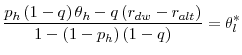(11)

or the point at which a bank is indifferent between going to the discount window and staying in the federal funds market. It is fairly easy to see that this critical value increases with a step-up in stigma, that is,

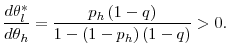$\displaystyle \frac{d\theta _{l}^{\ast }}{d\theta _{h}}=\frac{p_{h}\left( 1-q\right) }{% 1-\left( 1-p_{h}\right) \left( 1-q\right) }>0.$

(12)

It is then possible to see how the decision to go to the discount window changes with respect to the discount window rate. Interestingly, we see that

$\displaystyle \frac{d\theta _{l}^{\ast }}{dr_{dw}}=-\frac{q}{1-\left( 1-p_{h}\right) \left( 1-q\right) }<0$

(13)

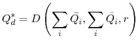
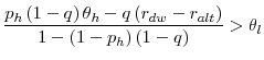
That is, if the discount window rate moves up, the critical value of the fixed cost for staying in the market goes down. Conversely, if the discount window rate goes down, the critical value for staying in the market goes up. In this way, a change in the discount window rate can create a separating equilibrium, where if there is a high discount window rate relative to the effective rate, then all banks stay in the federal funds market, but if the discount window rate falls, then those banks with the lowest fixed cost of going to the discount window do so, and only those with higher fixed costs stay in the market. Interestingly, this expression depends negatively on the discount window rate. That is, if the discount window rate is high, it is less likely to be satisfied and thus it is more likely that low fixed cost types are in the market. However, if the discount window rate is low, then it is more likely that the low cost types go to the discount window. As a result, the low types disagree, and drop out of the market. This implies that a fall in in the discount window rate can cause the number of participants in the federal funds market to decrease and cause discount window borrowing to increase.

If the low cost types borrow from the discount window and drop out of the market, then there are two opposing effects on the bargaining power of the remaining institutions. First, the increase in balances due to the discount window borrowing lowers the bargaining power of the sellers. However, at the same time, the existence of only the high cost types in the market raises the bargaining power of the sellers. To see how the bargaining power changes, the exit of some banks to the discount window in the proportion $\left( 1-p_{h}\right)$ implies that the effective amount of balances in the market is

$\displaystyle Q_{s}^{h}=Q_{s}+p_{l}Q_{s}$

(14)

Feeding this through into our expression for the relative bargaining power in the federal funds market shows that

$\displaystyle \frac{Q_{s}^{h}}{Q_{s}^{\ast }}=\frac{\left( 1+p_{l}\right) Q_{s}}{% Q_{s}^{\ast }}$

(15)

If $\frac{q}{\left( 1-q\right) }$ was the relative bargaining power of the buyers versus the sellers, this now becomes

$\displaystyle \frac{Q_{s}^{h}}{Q_{s}^{\ast }}=\frac{\frac{q\left( 1+p_{l}\right) }{1+qp_{l}% }}{1-\frac{q\left( 1+p_{l}\right) }{1+qp_{l}}}=\frac{z}{1-z}$

(16)

Because the distribution of types in the population is public knowledge, the bargaining problem continues only with the high cost types, and the new effective rate is

$\displaystyle r_{eff}^{\ast }=zr_{alt}+\left( 1-z\right) \left( r_{dw}+\theta _{h}\right)$

(17)

which, after a little algebra, can be shown to be higher than the effective rate in the perfect information case. It is also lower than the rate that the high cost types would pay at the discount window, assuming that

does not equal zero. In this way, a lowering of the primary credit rate can cause decreased participation in the federal funds market, higher federal funds rates, and increased primary credit borrowing. However, it also implies that total balances increase. Moreover, the total cost of borrowing is

$\displaystyle r_{funding}=r_{eff}^{\ast }Q_{s}+r_{dw}p_{l}Q_{s}$

(18)

which, with reasonable parameter values, could be lower than in the case where all banks stayed in the market, but funds rates were lower.

5 Empirical findings - aggregate data

As presented in the model above, there are likely two forces at work causing increased volume in trading above the primary credit rate. The first phenomenon is increased stigma. This would cause the fixed costs of going to the discount window to increase, and as a result, for any given spread of trading to the target rate, one would expect to see less discount window borrowing and more federal funds purchases than otherwise. The second is selection. Holding the distribution of costs of going to the discount window constant, one would still expect to see increased trading above the primary credit rate as the spread between the discount rate and the target rate is narrowed, if some portion of the distribution of costs is above the discount rate. No change in general credit conditions would be necessary to observe this phenomenon. If this were the case, then it is likely that there would be increased trading at selected spreads to the primary credit rate that is dependent on general measures of risk. In addition, if the influence of these measures of risk changes over time, one could interpret this as an indication of increased stigma.

The model above presents how either increases in stigma, or the decrease in the discount window rate which causes selection, can cause rates in the federal funds market to rise. The question is whether there was a secular increase in stigma during the crisis, or whether the phenomenon of increasing rates was simply a function of the selection bias inherent in the narrowing of the spread between the primary credit rate and the target federal funds rate. The analysis below suggests that it was likely a combination, and two empirical approaches are used to answer these questions. The first uses aggregate data, and addresses the question of whether a rise in stigma contributed to trading above the primary credit rate. The second uses DI-level data to evaluate whether there was selection bias in the federal funds market, independent of the any general increase in stigma that might have occurred. Each of these specifications are addressed in turn below.

5.1 Specification

"Stigma" is an unobservable cost of going to the discount window. Theoretical models and casual observation suggest that this cost could increase with a decrease in the health of banks, as they would become more reluctant to borrow from the discount window. To investigate this hypothesis a bit more closely, this section investigates the daily distributions of the federal funds rate to determine whether there was an increase in trading at relatively higher rates that is correlated with indicators of aggregate credit risk.

To this end, the following model is specified that examines the determinants of trading at selected spreads to the target rate. Let $V_{t}$ represent total federal funds market volume on date , and let $V_{it}$ represent volume brokered at selected ranges to the target rate. Furthermore, let $E\left( V_{it} \right )= \mu_{it}$ , where $\mu_{it}$ is specified as

$\displaystyle \mu_{it}=x_{t}\beta_{i} = \beta _{0}+\beta _{1ij}risk_{t}+\beta _{2ij}fftar_{t}+\beta _{3i}calendar_{t}$

(19)

The mean volume brokered at a particular spread to the target rate depends on number of factors, along with a vector of weights $\beta$ to be estimated below. The $\beta$ coefficients are allowed to vary both by the spread to the target for the trading volume,

, as well as the primary credit spread in effect,

, at time

. The factors used include $risk_{t}$ , which is a vector of indicators of general financial risk, $% fftar_{t}$ is the federal funds target rate, and $calendar_{t}$ is a vector of calendar effects.

With this specification in mind, there are two characteristics of the dependent variable that influence the chosen functional form. First, the dependent variable is strictly non-negative, suggesting that a transformation of the variable is appropriate. Second, there are a number of observations with the value of zero for which there is significant economic meaning, ruling out the usual log transformation. To address these issues, one can think of the dependent variable as the outcome of an experiment where, out of total brokered volume, volume brokered at rates a particular spread above the target rate "successes" and all other volume are "failures", or in other words, the outcome of a data generating process having a binomial distribution. The functional form becomes

$\displaystyle E\left(V_{it}\vert x_t,V_t \right) = V_{t} \Pr \left(x_t\beta_{i}\right)$

(20)

where $V_{it}$ is the volume brokered above a particular spread to the target federal funds rate, $V_{t}$ is total daily volume, and $\Pr ( )$ is the probability of success. The functional form of $\Pr ( )$ or "link function" is chosen to be a complementary log-log function, appropriate for modeling the maximum of a distribution. Newey-West errors that are corrected for heteroskedasticity and autocorrelation are used to control for these possible problems.

The analysis focuses on three ranges for brokered rates: trading that occurs more than 100 basis points above the target rate; greater than 50 basis up to 100 basis points above the target rate; and greater than 25 basis points up to 50 basis points. These series are plotted in figure 7. In addition to investigating volume at different spreads to the target rate, the $\beta_{ij}~$ coefficients allow for testing whether the effects of aggregate risk indicators change with the spread of the primary credit rate to the target rate. To this end, the sample is split into three periods: a baseline period from August 2006 to August 14, 2007, the day before the narrowing of the spread between the target and the primary credit rate; the period between August 17 and March 14, 2008, the day before the second spread narrowing; and March 17, 2008 to September 10, 2008. The sample has 525 daily observations.

If it were the case that stigma intensified, one might expect to see that aggregate indicators of risk or a deteriorating economy, were correlated with trading above the primary credit rate. Selected financial market variables that are used as explanatory variables in the analysis below are plotted in figure 8. These measures were all relatively elevated at some point in the sample, although not necessarily at the same time.

5.2 Results

As shown in table 3, there is some correlation between episodes of high-rate trading and measures of financial market volatility, and moreover, this correlation intensified as the crisis deepened and the spread of the discount rate to the target federal funds rate narrowed. Furthermore, the analysis also indicates that some factors associated with negative sentiment for the banking industry are also associated with high rate trading in the federal funds market. These results are consistent with the existence of stigma in obtaining a discount window loan. However, there are some differences in the correlations according to the portion of the federal funds distribution under investigation. These differences could be consistent with some selection issues, and are highlighted below.

More specifically, the results suggest that strained conditions in funding markets and negative sentiment towards banking organizations are associated with a greater share of volume brokered above the primary credit rate. As shown in the first line of the table, there is a positive correlation between the spread of the Treasury GC repo rate to the target federal funds rate and trading at selected spreads to the target in the first part of the sample. Some evidence suggests that repo rates and funds rates tend to move together over time, which explains their positive correlation. As the first year of the crisis wore on, however, the correlation between high rate trading and repo rates became slightly negative. In general, repo rates tend to fall with heightened demand for safe collateral, which occurs during periods of market stress. Taken together, then, the coefficient suggests that unsecured trading occurred at high rates at the same time that high-quality collateral was in demand.

Turning to the next set of coefficients, the results suggest that increases in the Libor-OIS spread was generally associated with higher rate trading in the federal funds market, but the effect differed according to the time period. In particular, the marginal effects suggest that overall, trading increased at rates greater than 100 basis points above the target rate, and rates 25 to 50 basis points above the target, but less so for the portion trades brokered at 50 to 100 basis points and above the target rate. However, the effects were somewhat modest, and the marginal effects attenuated as the crisis wore on. There are a few possible explanations for this result. First, the Libor panel incorporates rates only from a small sample of banks that also participate in the federal funds market. As a result, tensions for these particular institutions may not be a proxy for circumstances of all banks in the federal funds market.¹⁸ And third, the wide spread between Libor and OIS may have damped the marginal effect, suggesting that the elasticity of fed funds rates with respect to the Libor-OIS spread is not constant.

Overall stock price volatility as proxied by the S&P 500 VIX index appears to be correlated with high rate trading in the federal funds market, particularly for trades in the 25-50 basis point range and more so as the crisis intensified. In particular, there is some evidence of a correlation between high rate trading and stock price volatility at the upper end of the funds rate distribution that apparently moved little over the course of the crisis. However, as the crisis wore on, there was an increased correlation between stock price volatility and trading in the 25-50 basis point range.

Finally, the correlation between the CDS index and high rate trading was positive at the very top of the funds rate distribution, but negative for trading in the 50-100 basis point and 25-50 basis point ranges. This asymmetry could be consistent with stigma and selection in the federal funds market. That is, as the creditworthiness of borrowers declined, those institutions in better condition either borrowed from the discount window or were able to buy funds at rates below the primary credit rate. By contrast, less creditworthy institutions that remained in the federal funds market were forced to "pay up", and rates for these types of institutions increased.

The next rows control for various calendar effects. As shown repeatedly in other contexts, federal funds tend to trade firm on days when Fannie Mae and Freddie Mac make principal and interest payments on their mortgage-backed securities (MBS), on quarter-end dates, and on settlement days. Finally, the error in forecasting select factors on the Fed's balance sheet is not statistically significantly correlated with increased volume brokered at relatively high rates above the target rate. ¹⁹

To summarize, the results presented here suggest that some pickup in high rate trading was due to overall increases in financial risk. At the same time, the effects of increases in financial risk appear nonlinear, both across time and for the impact on different portions of the trading distribution. Selection in the funds market could contribute to this outcome. To this end, the next section examines the second hypothesis of the model, that is, whether there was selection in the federal funds market that resulted in an increased share of trading above the primary credit rate.

6 Empirical findings - bank-level data

The model above shows that funds rates paid are likely correlated with discount window borrowing. However, a simple regression with borrowing as an independent variable will not be appropriate, as the model illustrates that rates and borrowing are likely endogenously determined. Also, funds market participation likely exhibits selection: banks with higher stigma costs are more likely to remain in the federal funds market. The empirical strategy used below follows a framework outlined by Semykina and Wooldridge (2010) to control for these factors. Before proceeding to the selection results, the next two subsections provide information on the data construction, and to give a point of comparison, baseline panel regression estimates. The third and fourth subsections describe the test for endogeneity and selection, and the correction for endogeneity and selection, respectively.

6.1 Data construction

The data are constructed by combining DI-level daily data on rates paid in the federal funds market, reserve requirements, account activity, and borrowings from the discount window with daily information on key market variables, in addition to quarterly information from the Call and other regulatory reports issued on a less-frequent basis. Each piece is discussed in turn.

The data on federal funds rates is constructed using proprietary transaction-level data from the Fedwire Funds Service, using an algorithm pioneered by Furfine (1999) to match and form plausible overnight funding transactions, likely related to the federal funds market.²⁰ Similar data were used by Bartolini, Hilton and McAndrews (2010) and Afanso, Kovner, and Schoar (2010), to mention a few. Our sample is drawn from the universe of matched transactions from August 1, 2006 to September 11, 2008. The transaction data set contains basic transfer information, including the amount of the transaction, the implied interest rate of the identified transaction, and the seller and buyer in the trade. From there, these data are summarized on a daily basis, and the high rate on the day and the total funds bought are calculated.

Other DI-account activity variables are also constructed from proprietary Federal Reserve databases. The daylight overdraft information is also calculated from the same Fedwire funds transfer database. Peak daylight overdrafts, the variable used in the analysis, is the maximum amount a DI overdrafts its account at the Federal Reserve on a particular day. The data on reserve account balances are constructed from the Federal Reserve's database of DIs that report reserve balance and related information on the weekly "Report of Transaction Accounts, Other Deposits, and Vault Cash."²¹ Information on primary credit and TAF borrowings are also constructed from Federal Reserve internal databases.

The daily data are then paired with DI-level information from the Call and other regulatory reports that are issued on a less frequent basis, to capture key balance sheet and reserves-related items. Also included are some of the broader financial market indicators studied in section 5. After the combination of both datasets, the data are summarized by week and the estimation procedure is applied to the aggregated data. For the purposes of testing for selection, the sample is split into three periods: August 2006 to August 2007, when the primary credit rate was set 100 basis points above the target rate; August 2007 to March 2008, with a 50 basis point spread; and March 2008 to September 2008, with a 25 basis point spread. The sample ends at September 11, 2008, immediately before the failure of Lehman Brothers.

6.2 Baseline panel estimates and results

Before proceeding to the selection tests, it is instructive to have baseline panel regression results as a comparison. To this end, a panel regression of the form below is estimated:

$\displaystyle ffhighdev_{it}=c_{i} + \alpha_{t}primary_{it} + \beta_{t}TAF_{it} + \gamma days_{it} + x_{it}\delta + q_{t}\zeta + \epsilon_{it}.$

(21)

Summary statistics of all variables are in table 4. The dependent variable of interest is $ffhighdev_{it}$ , or the average of daily deviations of the highest observed rate for funds bought from the effective rate. Because the discount window generally served as a marginal source of funds in the sample period, the highest rate paid each day is probably the closest proxy to an actual reservation price. Comparing the highest rate paid to the effective rate gives an idea of a buying bank's rate paid relative to the market average. Averaging over a period shows how much a DI on average pays more than the market for its most expensive funds. It is constructed by calculating on a daily basis the deviation of entity 's highest rate paid in the federal funds market from the effective rate on the day. This rate is then averaged across the period corresponding to the spread of the primary credit rate to the target rate. As a result, the dependent variable measures the average of the peak rates paid, relative to the prevailing market average.

The first independent factor is $primary_{it}$ , which is the sum of primary credit borrowing by the DI over the specified period. The coefficient on this factor is permitted to vary over primary credit regimes. According to the model presented above, rates paid by these institutions should be lower than for institutions that did not go to the discount window. Also included in the list of independent variables is $TAF_{it}$ , which is the level of term auction credit held by the DI over the relevant week.

The next set of factors control for DI characteristics. The variable $days_{it}$ represents the number of days the DI participated in the federal funds market during that week. More or less frequent purchases may affect rates paid. The vector $x_{it}$ contains bank-specific information that varies over time, including information on assets and profitability measures. Should banks exhibit weakness on these counts, then it is likely that federal funds lenders would demand higher rates than would otherwise be the case.

As for the specification, a Hausman test rejects the hypothesis that a random effects model is sufficient to control for individual-level effects. As a result, fixed effects are assumed in the estimation.

The first column of table 5 presents the results. Primary credit borrowing does not appear to be significantly correlated with rates paid on federal funds. By contrast, daylight overdraft activity is correlated with higher fed funds rates, suggesting that banks with elevated funding demands are forced to pay more to obtain funds. TAF borrowing is also not significantly correlated with rates paid in the federal funds market, and the level of balances is also not correlated.

Some of the broad financial market variables are significantly correlated with rates paid in the federal funds market. Although the CDS index is somewhat surprisingly negatively correlated with trading in the federal funds market, the spread of the repo rate to the target rate, the Libor-OIS spread, the S&P 500 VIX and bank stock returns all have intuitive signs, as suggested from the aggregate analysis. As risk spreads widen, volatility increases, and stock returns fall, rates paid in the federal funds market rise.

The intercept terms, reported in the last three lines of the table, suggest that the high rates became higher as time wore on. In the 25 basis point regime, high rates were about 11 basis points higher on average than in the 100 basis point regime, after controlling for the factors listed above.

Despite these results, there is potentially endogeneity and selection in the model, which we address in the next section.

6.3 Estimation framework for testing and correction

Although the results in the previous section are informative, as illustrated by the model above, discount window borrowing is likely endogenous: Banks do not obtain discount window credit until federal funds rates go above their reservation price for borrowing at the discount window. As a result, parameter estimates on the effect of discount window borrowing are likely to be biased.

Semykina and Wooldridge (2010) develop a panel data estimator that controls for both endogenous regressors and selection bias. In the spirit of a traditional Heckman selection model, the diagnostic and estimation procedure is in three steps. Using the notation in Semykina and Wooldridge, in the first step, a probit model is estimated for each time period:

$\displaystyle Pr\left(s_{it}=1\vert z_{i}\right) = \Phi\left(z_{it}\delta^{a}_t+\bar{z}_{i}\xi_{t}^{a}\right)$

(22)

where $s_{it}$ equals 1 if the institution borrowed from the discount window, $z_{it}$ is a vector of exogenous variables, and $\bar{z_{i}}$ is the mean of these variables for each over all . Importantly, the $z_{it}$ should be observed regardless of whether the institution borrowed from the discount window. The means of exogenous variables $z_{it}$ control for unobserved fixed effects and are used to correct for possible selection bias.

The inverse Mills' ratios are then calculated, which take the form $\hat{\lambda}_{it}=\lambda \left(z_{it}\hat{\delta}_{t}^a + \bar{z_{i}}\hat{\xi}_{t}^a\right)$ . These will be used as a control function in the second stage.

Once the Mills' ratios are formed for each , the Mills' ratios are formed, the selection bias test can be executed. A fixed effects model two-stage least squares model is estimated only on the sample of institutions that borrowed from the discount window,

$\displaystyle ffhighdev_{it}=c_{i} + \alpha primary_{it} + x_{it}\beta_{t} + \gamma pcspread_{t} + \rho_{spread}\hat{\lambda}_{it} + \epsilon_{it1}.$

(23)

The coefficients $\rho$ differ by primary credit regime. Moreover, a subset $z_{it1} \subset z_{it}$ is used as instruments in the estimation. In this case, daylight overdrafts are the instrument for primary credit borrowing included in the $z_{it1}$ vector, and TAF borrowing is excluded from $z_{it1}$ but included in $z_{it}$ . This construct conforms to the Semykina and Wooldridge (2010) requirements that one instrumental variable is necessary to control for the endogenous regressor, and another is necessary to control for the selection. In the first stage, TAF borrowing, which was longer-term and for set periods, affects the probability of borrowing from the discount window in a given week. Daylight overdrafts, by contrast, occur during the operating day, and could be associated with the level of marginal discount window borrowing. Presumably, funds sellers would not know funds' buyers TAF or daylight overdraft activity, but both should be correlated with the decision to borrow from the discount window, or the level of discount window borrowing.

Selection bias is indicated by significant coefficients on the $\hat{\lambda}_{it}$ terms. If they are significant, pooled two-stage least squares is run on the following specification, which controls for both selection and endogeneity:

$\displaystyle fhighdev_{it}=c_{i} + \alpha primary_{it} + x_{it}\beta_{t} + \gamma pcspread_{t} + \bar{z}_{i}\eta + \rho_{spread}\hat{\lambda}_{it} + \epsilon_{it1}$

(24)

The $\alpha$ coefficient on the term should indicate the true relationship between rate paid on federal funds and discount window borrowing, while the $\rho_{spread}$ coefficients indicate the degree of selection according to time period.

6.4 Results

Selection in the federal funds market appears to have intensified as the spread between the primary credit rate and the target rate fell. As shown in the second column of table 5, the coefficient on $\rho_{25}$ terms suggest banks that borrowed from the discount window paid lower rates in the federal funds market. Put another way, an unobserved factor suggesting a higher propensity to borrow from the discount window is correlated with lower rates paid in the federal funds market. If this factor is "stigma," then lower stigma leads to lower fed funds rates paid. Consistent with the model's predictions, then, banks that were willing to borrow from the discount window did not pay as high rates for funds. The coefficient suggests that borrowing from the discount window was associated with about a 25 basis point decrease in the average high rate paid. In addition, there appears to be positive selection in the federal funds market when the spread is 100 basis points. Because this was the spread in a period of relative calm, it may be the case that borrowing from the window occurred on days with specific calendar-related pressures in the funds market, pushing up the correlation between funds rate trading and primary credit borrowing. The magnitude of the coefficient suggests that banks paid an average of about 30 basis points higher for high rate funds if going to the discount window during normal times. During the 50 basis point regime, the effect of going to the discount window on high rates paid was not significant.

However, examining the selection terms by themselves does not give a complete picture. As indicated by the coefficient on primary credit, borrowing $1 billion in primary credit is associated with a 32 basis point lower peak federal funds rate. Taken with the selection terms, the results suggest that borrowing from the discount window substantially reduced funding costs during the 25 basis point regime, somewhat damped them during the 50 basis point regime, and probably had a minimal net effect in the 100 basis point regime.

The final step of the estimation procedure corrects for both the endogeneity of primary credit, and the selection for federal funds rates. These results are presented in the final column of table 5. The coefficient on the primary credit term is negative and significant at the 7 percent level, suggesting that banks that borrowed primary credit paid lower federal funds rates. The point estimate suggests that for each $1 billion borrowed, peak rates fell by about 12 basis points. Taken with the highly statistically significant and negative coefficients on the selection terms, rates appear to be substantially lower for banks willing to go to the discount window. Indeed, during the 25 basis point regime, the net effect of borrowing $1 billion from the discount window was a peak funds rate that was about 40 basis points lower. Overall, the results are consistent with the model and suggest that DIs that borrowed from the discount window paid lower rates in the federal funds market, and this phenomenon became stronger as the primary credit rate spread narrowed and the crisis intensified.

One caveat to these results is that many of the control variables appear to be insignificant for the estimates that are corrected for selection. Some collinearity between the correction terms and the explanatory variables may explain this phenomenon.

Another caveat is the choice of dependent variable. Although the high rate paid on the day is a metric that is consistent with the model presented above, there may be some biases due to data limitations and also to using an extreme value of a distribution,. Other plausible suggestions include the 90th percentile of trades, expressed as a deviation from the effective rate, and measured over a week. Results with this dependent variable are shown in the final column of table 5. Specifically, while the coefficients on the selection terms remain significant and of consistent magnitude, the coefficient on the level of primary credit borrowing is no longer significant. The coefficients suggest that borrowing from the discount window led to rates that were about 7 to 9 basis points lower at the 90th percentile of the rate distribution. Although this is a lower point estimate than at the top of the distribution, one would expect this result a priori, as the 90th percentile is necessarily lower than the top of the distribution.

Although some point estimates are lower, factors including the number of days in the funds market becomes negative and significant, and some of the financial variables, including the spread of the repo rate to the target rate, become significant. In particular, an increase in the number of days in the federal funds market decreases the rate paid by about 2 basis points. This coefficient suggests that there could be some important relationship lending activities in the funds market, either brought about through size effects or through repeated interactions. In addition, the spread of the repo rate to the target rate remains negative and significant, suggesting that as collateralized lending becomes more important, the relative price of uncollateralized lending increases.

7 Conclusion

This paper presents a theoretical framework and empirical results that can explain the increase in trading in the federal funds market above the primary credit rate as the spread between the target rate and the primary credit rate narrowed in the first stages of the financial crisis. If banks differ on their aversion to obtaining funds from the discount window, a lower spread of the primary credit rate over the target rate can help sellers of funds price discriminate in a way that is not possible when the spread between the primary credit rate and the target is wider. And, although this price discrimination may have led to more high rate trading and trading above the primary credit rate, the welfare of sellers of federal funds may have increased. If welfare is measured by overall funding costs, the calculations in this paper suggest that these funding costs could have been trimmed as a result of the narrowing of the spread between the primary credit rate and the target rate.

Furthermore, the lowering of the primary credit rate may have helped trading in the federal funds market to continue despite the financial crisis, as sellers of funds were more able to price discriminate. Three salient empirical facts help to show this point: (1) as the spread between the primary credit rate and the target rate narrowed, the number of primary credit borrowers and the level of primary credit increased, while the number of participants in the federal funds market decreased; (2) on an aggregate level, trading above the primary credit rate is correlated with various measures of banking industry stress; and (3) on an institution-level, there is evidence of selection in the federal funds market - as the spread between the primary credit rate and the target rate narrowed, banks that did not go to the discount window paid significantly higher rates in the federal funds market.

By and large, most of the time fed funds were brokered below the primary credit rate and occasions where funds were brokered above the primary credit rate were infrequent. But it is still instructive to study these rare episodes of above-rate trading to understand the workings of this unsecured, overnight, interbank market.

Bibliography

Afanso, Gara, Kovner, Anna, and Schoar, Antoinette. , 2010.

"Stressed, not Frozen: The Federal Funds Market in the Financial Crisis," Federal Reserve Bank of New York Staff Report No. 437, March.

Armentier, Olivier, Ghysels, Eric, Sarkar, Asani, and Shradder, Jeffrey. 2010.

"Bank borrowing from the discount window and the TAF during the crisis," manuscript, Federal Reserve Bank of New York, August.

Artuc, Erhan, and Demiralp, Selva. 2010.

"Discount Window Borrowing after 2003: The Explicit Reduction in Implicit Costs," Journal of Banking and Finance, vol. 34, no. 4, p. 825-33.

Artuc, Erhan, and Demiralp, Selva. 2010.

"Provision of Liquidity through the Primary Credit Facility during the Financial Crisis: A Structural Analysis," FRBNY Economic Policy Review, August 2010, p. 43-53.

Bartolini, Leonardo, Hilton, Spence, and McAndrews, James J. 2010.

"Settlement Delays in the Money Market," Journal of Banking and Finance, vol. 34, no. 5, p. 934-945, May.

Bech, Morten L. and Klee, Elizabeth. 2009.

"The Mechanics of a Graceful Exit: Interest on Reserves and Segmentation in the Federal Funds Market," Federal Reserve Bank of New York Staff Report 416, December.

Bernanke, Ben S. , 2008.

"Liquidity Provision by the Federal Reserve," Remarks At the Federal Reserve Bank of Atlanta Financial Markets Conference, Sea Island, Georgia, May 18.

Calomiris, Charles. 1994.

"Is the Discount Window Necessary? A Penn Central Perspective," Federal Reserve Bank of St. Louis Review, p. 31-55, May-June.

Clouse, James and Dow, James P. 1999.

"Fixed Costs and the Behavior of the Federal Funds Rate," Journal of Banking and Finance, vol. 23, p. 1015-1029.

Dow, James P. 2001.

"The Recent Behavior of Adjustment Credit at the Discount Window," Journal of Macroeconomics, vol. 23, p. 199-211.

Ennis, Huberto, and Weinberg, John A. 2009.

"A Model of Stigma in the Fed Funds Market," working paper, Federal Reserve Bank of Richmond, June.

Furfine, Craig. 1999.

"The Microstructure of the Federal Funds Market," Financial Markets, Institutions, and Instruments, vol. 8, no. 5, p. 24-44.

Furfine, Craig. 2003.

"Standing Facilities and Interbank Borrowing: Evidence from the Fed's new discount window," International Finance, vol. 6, no. 3,pl 329-347.

Friedman, Milton, and Schwartz, Anna J. 1963.

A Monetary History of the United States. Princeton: Princeton University Press.

Goodfriend, Marvin. 1983.

"Discount window borrowing, monetary policy, and the post-October 6, 1979 Federal Reserve operating procedure," Journal of Monetary Economics, p. 343-356, September.

Madigan, Brian and Nelson, William. 2002.

"Proposed Revision to the Federal Reserve's Discount Window Lending Programs," Federal Reserve Bulletin, p. 312-319, July.

Peristiani, Stavos. 1998.

"The Growing Reluctance to Borrow at the Discount Window: An Empirical Investigation," The Review of Economics and Statistics, p. 611-620.

Semykina, Anastasia, and Wooldridge, Jeffrey M. , 2010.

"Estimating panel data models in the presence of endogeneity and selection," Journal of Econometrics, forthcoming.

Thornton, Daniel L. 2008.

"Walter Bagehot, the discount window and TAF," Economic Synopses, Federal Reserve Bank of St. Louis, no. 27.

White, Eugene N. 1983.

The Regulation and Reform of the American Banking System, 1900-1929. Princeton: Princeton University Press.

Wooldridge, Jeffrey., 1995.

"Selection Corrections for Panel Data Models Under Conditional Mean Independence Assumptions," Journal of Econometrics, vol. 68, p. 115-132, July.

**Figure 1:** **Primary credit and the federal funds rate, monthly averages**
Accessible Version

**Figure 2:** **Primary credit, total balances, and high fed funds rate**
Accessible Version

**Figure 3:** **Primary credit and federal funds volume**
Accessible Version

**Figure 4:** **Primary credit and fed funds market participation**
Accessible Version

**Figure 5:** **Distribution of brokered federal funds rates**
Accessible Version

**Figure 6:** **Lowering the primary credit rate**
Accessible Version

**Figure 7:** **Trading above the target rate**

Accessible Version

**Figure 8:** **Selected financial market indicators**

Accessible Version

Table 1 (part 1 of 3): Discount window cost

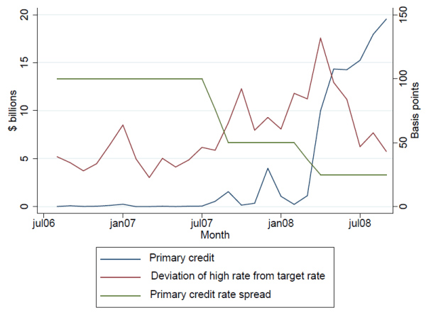
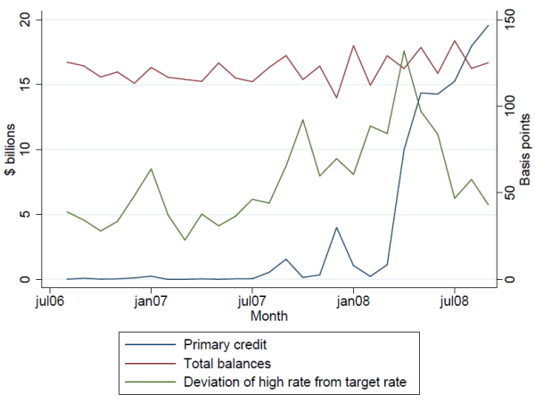
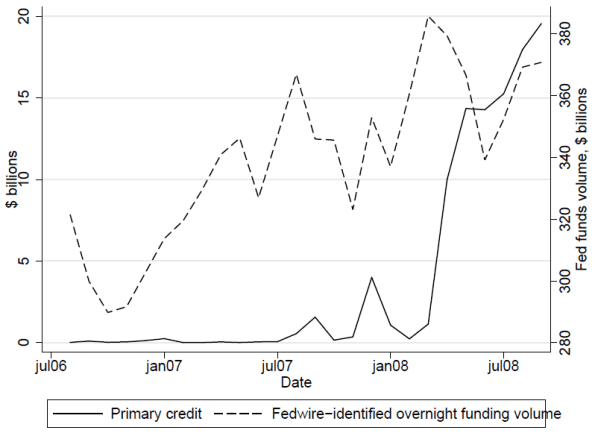
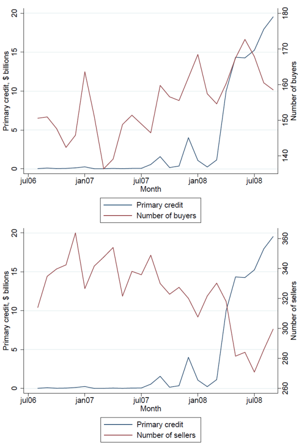
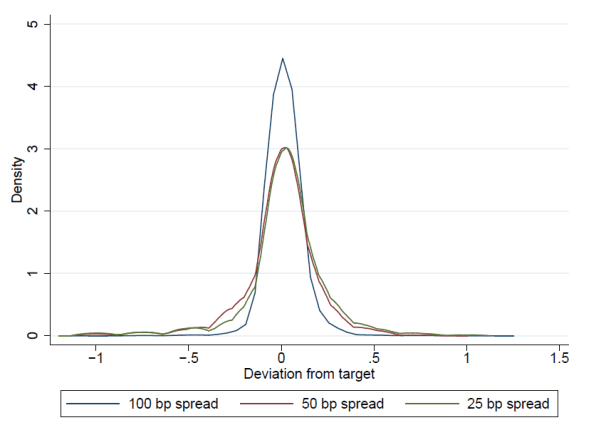
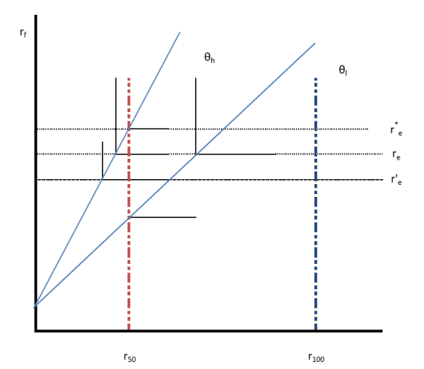
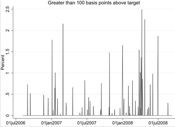
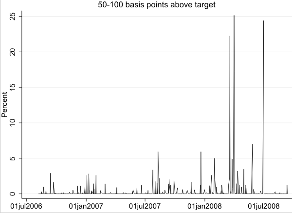
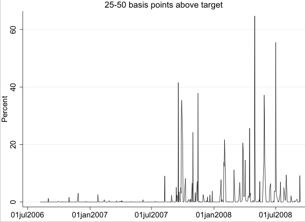
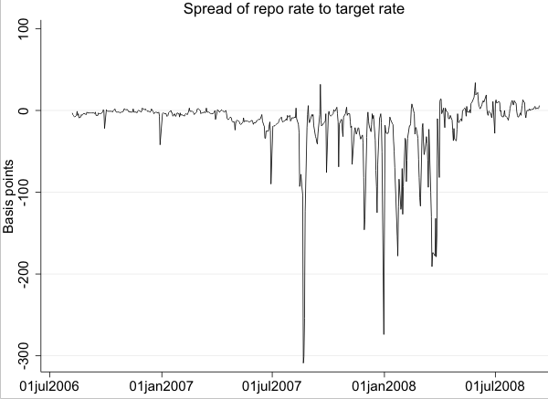
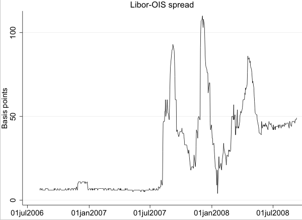
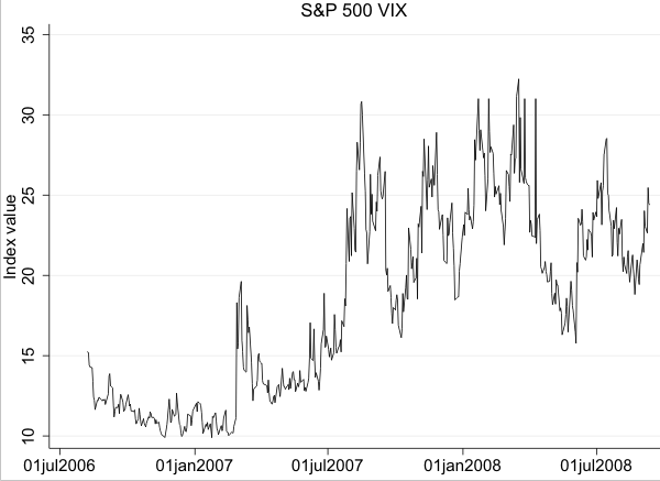
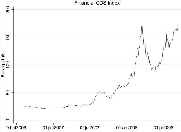
DI	Stigma cost	Discount window cost when primary credit spread is*: 100	Discount window cost when primary credit spread is*: 50	Discount window cost when primary credit spread is*: 25
A	0	100	50	25
B	10	110	60	35
C	40	140	90	65

*Discount window cost=primary credit spread + stigma cost

Total borrowing cost=target federal funds rate + discount window cost

Table 1 (part 2 of 3): Discount window cost Suppose federal funds is trading 55bp above the target rate ...

DI	Stigma cost	When the spread is X, borrow from window or buy in market?: 100	When the spread is X, borrow from window or buy in market?: 50	When the spread is X, borrow from window or buy in market?: 25
A	0	Market	Window	Window
B	10	Market	Market	Window
C	40	Market	Market	Market

Table 1 (part 3 of 3): Discount window cost ... what happens to the federal funds market and to funding costs?

	100	50	25
Average rate for trades	55	60	65
Funds market volume (percent)	100	66	33
Average funding costs*	55	57	38

*Average funding costs are only for these high-rate trades.

All values expressed in basis points

Window = Borrow from discount window

Market = Buy funds in market

Table 2: **Trading at high rates in the federal funds market (Percent)**
	Average spread between high and target rate	Percent of days: 100	Percent of days: 50-100	Percent of days: 25-50	Percent of brokered volume: 100	Percent of brokered volume: 50-100	Percent of brokered volume: 25-50
Aug 1, 2006 to Aug 14, 2007	38	8	19	10	0.04	0.14	0.06
Aug 17, 2007 to March 14, 2008	69	12	29	42	0.05	0.30	1.76
March 17, 2008 to Sep 10, 2008	82	12	25	56	0.12	0.79	3.10

Table 3: **Federal funds trading at selected spreads above target rate**
	Above 100bp: Parm.	Above 100bp: Marg. eff.	50-100bp: Parm.	50-100bp: Marg. eff.	25-50bp: Parm.	25-50bp: Marg. eff.
Spread of repo rate to target rate	1.778	0.115	5.016	2.385	16.227	27.688
Spread of repo rate to target rate (Newey-West Error)	(1.52)	(0.10)	(0.45)	(0.16)	(2.99)	(5.22)
Spread of repo rate to target rate, August 17-March 14	-2.411	-0.156	-5.047	-2.400	-16.292	-27.800
Spread of repo rate to target rate, August 17-March 14 (Newey-West Error)	(1.41)	(0.09)	(0.40)	(0.16)	(2.99)	(5.20)
Spread of repo rate to target rate, March 14-September 11	-1.854	-0.120	-5.689	-2.705	-16.882	-28.806
Spread of repo rate to target rate, March 14-September 11 (Newey-West Error)	(1.71)	(0.11)	(0.54)	(0.16)	(3.03)	(5.32)
Libor-OIS spread	-23.087	-1.493	4.693	2.232	11.906	20.316
Libor-OIS spread (Newey-West Error)	(9.93)	(0.65)	(0.58)	(0.29)	(1.89)	(3.10)
Libor-OIS spread, August 17-March 14	20.356	1.316	-4.187	-1.991	-13.525	-23.078
Libor-OIS spread, August 17-March 14 (Newey-West Error)	(10.02)	(0.65)	(0.67)	(0.33)	(1.98)	(3.20)
Libor-OIS spread, March 14-September 11	24.016	1.553	-7.750	-3.685	-11.173	-19.065
Libor-OIS spread, March 14-September 11 (Newey-West Error)	(10.45)	(0.68)	(0.96)	(0.36)	(2.31)	(3.74)
S&P 500 VIX	12.017	0.777	2.819	1.340	-12.001	-20.477
S&P 500 VIX (Newey-West Error)	(6.02)	(0.39)	(4.07)	(1.93)	(7.92)	(13.37)
S&P 500 VIX, August 17-March 14	-10.631	-0.687	12.424	5.908	8.662	14.781
S&P 500 VIX, August 17-March 14 (Newey-West Error)	(5.78)	(0.38)	(3.97)	(1.89)	(9.13)	(15.38)
S&P 500 VIX, March 14-September 11	-10.670	-0.690	-1.924	-0.915	26.406	45.058
S&P 500 VIX, March 14-September 11 (Newey-West Error)	(5.61)	(0.36)	(4.07)	(1.95)	(8.82)	(14.57)
CDS index	-19.895	-1.286	4.932	2.345	6.791	11.588
CDS index (Newey-West Error)	(6.58)	(0.44)	(1.72)	(0.84)	(2.54)	(4.27)
CDS index, August 17-March 14	21.179	1.369	-5.507	-2.619	-8.669	-14.792
CDS index, August 17-March 14 (Newey-West Error)	(6.39)	(0.43)	(1.71)	(0.84)	(2.51)	(4.22)
CDS index, March 14-September 11	16.211	1.048	-5.281	-2.511	-9.507	-16.221
CDS index, March 14-September 11 (Newey-West Error)	(6.30)	(0.42)	(1.76)	(0.80)	(2.60)	(4.33)
Target federal funds rate	1.571	0.102	0.015	0.007	-1.603	-2.735
Target federal funds rate (Newey-West Error)	(0.34)	(0.02)	(0.12)	(0.06)	(0.34)	(0.64)
Target federal funds rate, August 17-March 14	-0.951	-0.061	-0.261	-0.124	1.248	2.129
Target federal funds rate, August 17-March 14 (Newey-West Error)	(0.40)	(0.03)	(0.07)	(0.03)	(0.16)	(0.33)
Target federal funds rate, March 14-September 11	2.128	0.138	2.481	1.180	-0.343	-0.586
Target federal funds rate, March 14-September 11 (Newey-West Error)	(0.87)	(0.05)	(0.47)	(0.17)	(0.62)	(1.07)
Calendar effects, Month begin	-13.276	-0.858	1.991	0.947	2.181	3.722
Calendar effects (Newey-West Error)	(0.81)	(0.07)	(0.41)	(0.19)	(0.24)	(0.34)
Calendar effects, P&I day	0.615	0.040	0.425	0.202	1.004	1.713
Calendar effects, P&I day (Newey-West Error)	(0.28)	(0.02)	(0.18)	(0.09)	(0.11)	(0.16)
Calendar effects, Month end	1.276	0.082	1.325	0.630	1.774	3.026
Calendar effects, Month end (Newey-West Error)	(0.52)	(0.03)	(0.15)	(0.08)	(0.38)	(0.59)
Calendar effects, Quarter end	1.702	0.110	2.438	1.159	0.194	0.332
Calendar effects, Quarter end (Newey-West Error)	(0.94)	(0.06)	(0.35)	(0.13)	(0.92)	(1.58)
Calendar effects, Settlement day	1.997	0.129	0.446	0.212	0.254	0.434
Calendar effects, Settlement day (Newey-West Error)	(0.39)	(0.03)	(0.31)	(0.15)	(0.11)	(0.18)
Calendar effects, FOMC meeting	-0.847	-0.055	2.204	1.048	1.388	2.368
Calendar effects, FOMC meeting (Newey-West Error)	(1.06)	(0.07)	(0.29)	(0.13)	(0.16)	(0.32)
Factors miss	-0.168	-0.011	-0.010	-0.005	0.264	0.451
Factors miss (Newey-West Error)	(0.18)	(0.01)	(0.05)	(0.02)	(0.10)	(0.17)
Constant	-11.862		-9.208		-0.326
Constant (Newey-West Error)	(1.24)		(0.57)		(1.67)
N	525		525		525

Dependent variable is daily brokered volume in $billions.

Newey-West heteroskedastic-autocorrelated corrected errors in parentheses.

significant at 5 percent level.

Table 4: **Summary statistics**
	Mean	Std. dev.	Min	Max
100bp regime	0.50	0.50	0	1
50bp regime	0.28	0.45	0	1
25bp regime	0.23	0.42	0	1
Primary credit	0.01	0.34	0	17.5
100bp regime	0.00	0.01	0	1.16
50bp regime	0.00	0.09	0	15
25bp regime	0.01	0.33	0	17.5
Peak daylight overdrafts	0.31	2.82	0	96.58
TAF borrowing	0.14	1.82	0	73.19
Daily total balances	0.01	0.08	0	7.18
Days in market	0.62	1.48	0	5
Funds bought	0.31	2.82	0	92.92
Assets	1.42	23.42	0	1392.27
Required reserves	0.03	0.25	0	7.89
CDS financial index	0.60	0.45	0.21	1.69
Spread of repo rate to target rate	-15.75	33.13	-221	26.25
Libor-OIS spread	27.72	24.69	5.41	106.90
S&P 500 VIX	18.12	5.78	10.19	30.02
Return on bank stocks	-0.30	1.41	-8.67	3.81
N	120464

Table 5: **Controlling for selection bias in discount window borrowing**
	Panel	Selection test	Corrected estimates	Corrected estimates (90th percentile)
Primary credit	2.842	-32.364**	-12.083+	-0.850
Primary credit (Standard Error)	(4.98)	(12.23)	(6.87)	(1.84)
Primary credit, 50bp regime	-2.048
Primary credit, 50bp regime (Standard Error)	(5.13)
Primary credit, 25bp regime	-2.407
Primary credit, 25bp regime (Standard Error)	(4.90)
Peak daylight overdrafts	0.838**
Peak daylight overdrafts (Standard Error)	(0.24)
TAF borrowing	-0.024
TAF borrowing (Standard Error)	(0.06)
Daily total balances	-1.554	-36.269+	-14.744	-0.719
Daily total balances (Standard Error)	(1.89)	(21.77)	(16.68)	(6.24)
Days in market	-0.096	5.658	0.473	-2.177**
Days in market (Standard Error)	(0.11)	(3.52)	(1.01)	(0.42)
Funds bought	0.239	-2.921+	-1.179	-0.184
Funds bought (Standard Error)	(0.15)	(1.53)	(1.07)	(0.36)
Assets	-0.001	-0.099	-0.066	-0.008
Assets (Standard Error)	(0.00)	(0.07)	(0.06)	(0.02)
Required reserves	3.516	38.295	39.492	13.043
Required reserves (Standard Error)	(3.22)	(23.83)	(25.17)	(8.24)
CDS financial index	-4.845**	-20.566	-13.366+	-5.305+
CDS financial index (Standard Error)	(0.47)	(13.70)	(7.65)	(2.92)
Spread of repo rate to target rate	-0.054**	0.150	0.011	-0.076**
Spread of repo rate to target rate (Standard Error)	(0.00)	(0.11)	(0.06)	(0.03)
Libor-OIS spread	0.015**	-0.103	-0.002	0.069
Libor-OIS spread (Standard Error)	(0.01)	(0.18)	(0.11)	(0.05)
S&P 500 VIX	0.290**	0.742	0.216	0.600
S&P 500 VIX (Standard Error)	(0.04)	(1.13)	(0.55)	(0.38)
Return on bank stocks	-0.135**	0.666	-0.148	0.068
Return on bank stocks (Standard Error)	(0.06)	(1.47)	(0.80)	(0.36)
Selection terms, 100bp regime		30.581**	11.435	-1.460
Selection terms, 100bp regime (Standard Error)		(13.71)	(8.02)	(2.34)
Selection terms, 50bp regime		-2.046	-11.713**	-8.955**
Selection terms, 50bp regime (Standard Error)		(7.15)	(5.10)	(2.63)
Selection terms, 25bp regime		-25.929**	-24.780**	-6.981**
Selection terms, 25bp regime (Standard Error)		(10.77)	(11.62)	(3.43)
Fixed effects, TAF			0.074+	0.600
Fixed effects, TAF (Standard Error)			(0.04)	(1.21)
Fixed effects, Days in market			-0.005	-2.177**
Fixed effects, Days in market (Standard Error)			(0.01)	(0.42)
Fixed effects, Funds bought			2.312	0.249
Fixed effects, Funds bought (Standard Error)			(1.60)	(0.64)
Fixed effects, Assets			0.046	0.005
Fixed effects, Assets (Standard Error)			(0.03)	(0.01)
Fixed effects, Required reserves			-0.000	0.000
Fixed effects, Required reserves (Standard Error)			(0.00)	(0.00)
Fixed effects, Daily total balances			-25.355	-6.293
Fixed effects, Daily total balances (Standard Error)			(28.72)	(13.72)
Constant	2.021**	-39.438	-20.226	7.577
Constant (Standard Error)	(0.76)	(27.07)	(19.96)	(6.65)
Constant, 50bp regime	6.351**	90.681**	63.867**	18.951+
Constant, 50bp regime (Standard Error)	(0.50)	(34.81)	(25.64)	(10.40)
Constant, 25bp regime	10.686**	144.678**	100.504**	20.351
Constant, 25bp regime (Standard Error)	(0.65)	(50.63)	(45.44)	(13.72)
Adjusted R-squared	0.168		.
N	21,363	641	641	641

Dependent variable is the deviation of the average observed high rate paid for federal funds from the effective rate.

Cluster-robust standard errors in parentheses on panel and selection estimates.

Bootstrapped standard errors on corrected estimates.

+ significant at 10 percent level; ** significant at 5 percent level.

Footnotes

* Board of Governors of the Federal Reserve System, Mail Stop 59, 20th and C Streets, Washington, DC 20551. Tel: (202) 721-4501. Email: [email protected]. The views expressed in this paper are those of the author and not necessarily those of the Board of Governors, other members of its staff or the Federal Reserve System. Thanks to Seth Carpenter, Jim Clouse, Jane Ihrig, Ruth Judson, Ed Nelson and Viktors Stebunovs for helpful comments. Amanda McLean and Ari Morse provided excellent research assistance. Return to Text

1. Federal Reserve Board Press Release, August 17, 2007. Return to Text

2. Federal Reserve Board Press Release, March 16, 2008. Return to Text

3. The Federal Reserve implements monetary policy by influencing conditions in the federal funds market so that the average rate in that market (the "effective" federal funds rate) trades close to the target rate. Return to Text

4. Although there were some instances of trading above the primary credit rate before the beginning of the financial crisis, the incidence was much less frequent. Return to Text

5. Calomiris (1994) empirically examines a related issue, the spreads on commercial paper as a result of the Fed's discount window lending during the Penn Central crisis. The lending in question, however, was to a non-DI, and in today's parlance, would have likely fallen under the auspices of the Commercial Paper Funding Facility (CPFF) or a direct loan to a non-bank counterparty, rather than the investigation of Fed lending to DIs that is examined here. Return to Text

6. Artuc and Demiralp (2010) extended this work to investigate the effectiveness of discount window credit in the financial crisis; they concluded that it helped to dampen federal funds market volatility. Return to Text

7. Technically, clearing balance requirements can also be considered a policy tool for the period studied in this paper. Return to Text

8. More recently, there have been additions to the set of tools available for monetary policy implementation such as the payment of interest on required reserve balances and excess balances. This paper does not address these changes. Return to Text

9. These claims implicitly abstract from the ability of a DI to change its balance sheet composition so as to affect its reserve requirement. For example, instead of buying federal funds, a DI could satisfy its reserve requirement by attracting new deposits, selling a security, or terminating a loan. All of these balance sheet management measures can bring new cash to the DI so as to make it easier to satisfy a reserve requirement. Return to Text

10. The discouragement of longer-term borrowing has been evident for much of the discount window's history; this characteristic was not unique to the period discussed here. Return to Text

11. For more details, refer to http://www.frbdiscountwindow.org/programs.cfm?hdrID=14 Return to Text

12. Sidel, Robin, Ip, Greg, and Bauerlein, Valerie. 2007. "Banks Step Up to Fed's Window," The Wall Street Journal, August 23, p. A3. Return to Text

13. The total borrowing cost is the discount window cost plus the target federal funds rate. For simplicity, one can assume that the target rate is the same in all cases; as such, all calculations depend only on the spread. Return to Text

14. Moreover, there is no discounting between period 2 and period 3. Return to Text

15. Goodfriend (1983) modeled the decision to borrow from the discount window in part as a function of these costs. Return to Text

16. Implicitly, this assumes that there is no correlation between seller and buyer status and willingness to go to the discount window, that is, $\Pr \left( \theta _{i}=\theta _{h}\vert q_{i}<\bar{q}_{i}+\hat{q}_{i}\right) =\Pr \left( \theta _{i}=\theta _{h}\vert q_{i}>\bar{q}_{i}+\hat{q}_{i}\right)$ Return to Text

17. The model could be extended to include banks that actually derive utility from going to the discount window, but we do not address this point here. Return to Text

18. The reporting of these rates came under question during the period studied in this paper; news reports suggested that banks were under-reporting rates. Refer to Carrick Mollenkamp and Mark Whitehouse, "Study casts doubt on key rate: WSJ analysis suggests banks may have reported flawed interest rate data for Libor," The Wall Street Journal, May 29, 2008, p. A1 Return to Text

19. Each day, staff at the Federal Reserve Bank of New York and the Federal Reserve Board forecast the level of balances supplied by various factors on the balance sheet, including check float, currency in circulation, and the Treasury's cash balance at the Federal Reserve. The "forecast miss" is the error in this forecast, in billions of dollars. Return to Text

20. The algorithm matches an outgoing Fedwire funds transfer sent from one account and received by another with a corresponding incoming transfer on the next business day sent by the previous day's receiver and received by the previous day's sender. This pair of transfers is considered a federal funds transaction if the amount of the incoming transfer is equal to the amount of the outgoing transfer plus interest at a rate consistent with the rates reported by major federal funds brokers. However, because we have no independent way to verify if these are actual federal funds transactions, our identified trades and characteristics of these trades are subject to error. Return to Text

21. This reporting form is known as the FR2900, and can be found on the Federal Reserve's website. Return to Text

^♣ This version is optimized for use by screen readers. Descriptions for all mathematical expressions are provided in LaTex format. A printable pdf version is available. Return to Text