Skip to: [Printable Version (PDF)] [Bibliography] [Footnotes]

Finance and Economics Discussion Series: 2011-56 Screen Reader version ^♣

The Usefulness of Core PCE Inflation Measures¹

Alan Detmeister²

Friday, 20 January 2012

Keywords: Inflation, core prices.

Abstract:

This paper examines a number of alternative PCE price inflation measures including overall PCE inflation, PCE inflation excluding food and energy, trimmed mean PCE inflation, component-smoothed inflation, variance-weighted inflation, inflation with weights based on disaggregated regressions, and survey measures of inflation expectations. When averaging across a handful of specifications based on the primary uses of a core inflation measure three conclusions arise: 1. Inflation rates for nearly all the measures best track ex-post trend inflation or predict future overall inflation when they are averaged over a considerable number of months. Overall PCE price inflation should be averaged over 18 months or longer. A shorter averaging period is appropriate for core measures, often on the order of 12 months. 2. Even after appropriately averaging each index, core inflation indexes generally perform better than overall inflation. 3. Exclusion indexes, such as PCE excluding food and energy, perform slightly worse than many other possible core inflation measures; trimmed mean PCE, or a variance-weighted index, may be better choice for a summary inflation measure

JEL Classification:E31, E37

Introduction

Consumer welfare depends on overall consumer prices, but price changes for the aggregate basket of goods and service purchased by consumers vary widely from quarter to quarter and from year to year. Faced with this volatility, many economists and policymakers have sought a measure which reduces the transitory volatility of overall inflation while maintaining its essential properties. The core inflation measures resulting from this quest perform a variety of roles including: a real-time summary measure of current inflation excluding transitory factors, a guide for future movements in overall inflation, and, in some countries, an intermediate target for monetary policy. A measure which performs well in one of these roles may not be well suited for the other roles. Nonetheless, for clarity of communication a single measure of inflation may be preferred to several measures each focused on a different role.

Just as there are multiple uses of core inflation measures, there are multiple ways to construct one. The most popular US core inflation measure, consumer price inflation excluding food and energy, is an exclusion index-it excludes some items and takes the weighted average inflation rate of the remaining items. Alternative approaches to constructing core inflation abound. These include, but are not limited to, trimmed means, persistence weighting, variance weighting, component smoothing, exponential smoothing, and dynamic factors.

From an empirical perspective these various core inflation measures are useful only if they provide something that cannot be found in the overall inflation measure, for example, if the core measure is a better predictor of future overall inflation, or if the core measure better matches in real time an ex-post measure of current trend overall inflation. If the core measure cannot perform these tasks better than overall inflation over a significant period of time then there is little reason to use it.

This note examines a number of measures of core inflation to provide guidance to the media, policymakers, and researchers about which measures may be the most useful to follow. In many ways this note is an expansion of Rich and Steindel (2007) and other examinations of US core inflation measures.³ Rich and Steindel selected a small group of the most common exclusion and trimmed mean inflation indexes and compared the ability of these measures to track trend and predict future overall inflation using quarterly data. They concluded that no one index is clearly preferred over the other indexes. This note builds on Rich and Steindel's results, and results from other core inflation comparisons, by examining a larger set of core inflation measures over a wider span of sampling intervals and time periods. Combining results across many different specifications leads to three main conclusions:

Most of the measures perform substantially better in predicting future overall inflation or in tracking an ex-post measure of trend inflation when their inflation rates are averaged over a number of months. For overall PCE inflation the appropriate interval is on the order of 18 months or more. For the best-performing measure, the Dallas Fed trimmed mean, the preferred sampling interval is the inflation rate over the most recent 15 months. This result casts doubt on the information content of one-, three-, and perhaps even six-month inflation rates.
At most intervals, particularly short sampling intervals, nearly all of the core measures track ex-post trend inflation or predict future inflation considerably better than overall PCE. Even when appropriately averaged most of the tested core inflation measures still perform better than overall PCE inflation, though the difference is much smaller. This suggests that core inflation measures remain a useful concept.
Exclusion indexes, including PCE excluding food and energy, perform somewhat worse than other core measures, but the difference is often small. Nonetheless, this suggests that if we desire a single core inflation measure then there may be better choices than PCE excluding food and energy. The trimmed mean and variance weighted measures perform particularly well.

Types of core inflation measures

Since at least the 1970s, the overall consumer price index published by the Bureau of Labor Statistic in the US has been recognized to be susceptible to swings caused by large movements in a few items. Up and down swings in the prices of a handful of items leads to substantial short-term volatility in the inflation index. Over the past few decades a large number of different core inflation measures have been advanced to reduce this transitory volatility while still maintaining the signal of longer-run inflation movements.

For the most part, these core measures of inflation are rule-based recombinations of the price changes observed in the overall price index and serve as a tool for communicating the stance of current or future inflation in real-time. This paper will follow that convention and define a core inflation measure as a rule-based recombination of the data used to construct the PCE price index that can be followed each month as the data is released.⁴ Thus a core inflation measure is not the outcome of a model which includes information not in the primary consumer price data, such as asset prices, wages, exchange rate changes, estimates of the output gap, or the judgmental forecasts of experts. Inclusion of information from those items may help provide a better forecast of inflation, but, by their very nature and complexity, they would be less useful in communication. As a result, a core inflation measure is not substitute for a fully-specified forecast of inflation, though it is sometimes used as one informally.

As noted above, the most common core inflation measures are exclusion indexes. They are constructed by identifying a handful of items which are considered to be the cause of the excess volatility and then building a new price index which excludes those same items throughout history. The most popular exclusion index is consumer price inflation excluding food and energy, though official agencies in the United States construct many additional exclusion indexes, and other countries sometimes use different exclusion indexes.⁵

The most common core inflation measures after exclusion indexes are central tendency statistical measures such as the trimmed mean and weighted median. These indexes were developed by Bryan and Pike (1991) and Bryan and Cecchetti (1994) for the US CPI and later by Dolmas (2005) for the US PCE price index. These indexes are based on the idea that given the structure of the price changes, large changes in a few items can cause excess movement in the average price level. As a result, the items with the largest positive and negative prices change in the month are removed. These indexes differ from exclusion indexes in that the items removed can change each month, whereas the same items are removed every month in exclusion indexes. Following the recommendations of Cecchetti and Bryan, the Federal Reserve Bank of Cleveland each month removes the 16 percent of consumption bundle with the largest price increases and the 16 percent of the consumption bundle with the largest price decreases (or smallest price increases) when creating the trimmed mean price index for the US CPI. Different trim points are used by the Federal Reserve Bank of Dallas when creating the trimmed mean PCE index. In contrast, the weighted median inflation rate removes all except the single item at the center of the distribution of price changes.

Several additional methods of creating core inflation have been suggested. Some of these are based on re-weighting items in the index in a less discrete fashion than the exclusion and trim measures, which simply include or exclude an item. For example, a variance-weighted inflation index lowers the weight placed on highly volatile items and raises the weights placed on low volatility ones. A regression-based price index uses component weights determined by a regression for predicting overall inflation from the disaggregated components. The cost-of-nominal distortions price index (CONDI) places more weight on items which tend to change price less frequently.

Some other methods do not reweight the subcomponents of the inflation index but merely smooth the inflation rate over time following a formula. Examples following this technique that are examined in this roundup include Cogley's exponentially-smoothed inflation (Cogley 2002), and the prediction of Stock and Watson's UC-SV model (Stock and Watson 2008), both of which are weighted averages of past overall inflation. A component smoothed index smoothes the price changes of the individual items over time before the individual items are aggregated to find a top line inflation index. Highly volatile items are smoothed more than low volatility items.

Table 1 lists the various inflation measures examined in this note with a very brief description of each. A more detailed description of some of the measures is contained in the appendix. Silver (2007) and Wynne (2008) provide additional background on different types of core inflation measures.

This list of core measures examined in this note is large, but it is not comprehensive. Measures not listed on table 1 or examined in this note include indexes based on persistence weights, which have not fared well in other comparisons Clark 2001; Cutler 2001; Bilke and Stracca 2007; Smith 2007); and measures which are likely to be too complex for use in communication with the general public such as dynamic factor indexes (Cecchetti 1997; Kapetanios 2004; Reis and Watson 2007; Giannone and Matheson 2007), common trends (Bagliano and Morana 2003), forecasts from multi-equation models of overall inflation (Folkertsma and Hubrich 2001; Domenech and Gomez 2006; Velde 2006) and other techniques (Arrazola and de Hevia 2002).

Also included in the round-up of measures in this note are values from inflation expectations surveys. Specifically, inflation expectations from the Reuters/University of Michigan Survey of Consumers are examined. Other inflation expectations surveys lack the history or frequency needed for inclusion here. Unlike the other measures examined in this note, inflation expectations are not re-combinations of actual inflation data and hence are not truly core inflation measures, but rather they are averages of what individuals expect inflation to be. Nonetheless, the growing prominence of inflation expectations as an anchor for the inflation process suggests that including expectations in this round-up is merited. Additional support for including expectations comes from Ang, Bekaert, and Wei's (2007) finding that survey measures of inflation expectations out-perform some conventional measures of core inflation.

This note focuses on inflation in the United States personal consumption expenditures price index (PCE prices) published by the Department of Commerce's Bureau of Economic Analysis.⁶ Much of the data used in constructing the PCE price index comes directly from to the more well-known Consumer Price Index (CPI) published by the Department of Labor's Bureau of Labor Statistics, and the two price indexes generally follow each other, so the main results of this paper would likely apply to CPI inflation measures as well.

In constructing the different core inflation measures used in this paper, out-of-sample methods are used whenever possible.⁷

An overview of the individual tests of core inflation

Different studies have proposed a large number of desirable criteria for a core inflation measures, but this study confines the evaluation criteria to three varieties of tests of tracking trend inflation or predicting future inflation. These tests derive from the most common uses for a core inflation measure, and therefore are the most important criteria on which to judge a core inflation measure.⁸

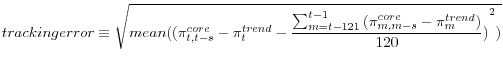
1. The first test flows from the use of core inflation to measure the current inflation rate purged of transitory factors. In this context underlying inflation (and hence the core inflation measure) should closely track an ex-post estimate of trend inflation. Such ex-post estimates of trend inflation are generally constructed using a band-pass filter, a Hodrick-Prescott filter, or a 36-month centered moving average of headline inflation.⁹

2. The second test derives from the use of core inflation measures to informally suggest where overall inflation will move to in the coming period. In this context headline inflation is considered to be volatile and mean-reverting to underlying inflation. As a result underlying inflation (and hence the core inflation measure) should be a good predictor of future overall inflation.

3. The third test derives from the Phillips curve often used in more formal inflation forecasting. Like the second test this one also uses core inflation to predict overall future inflation, but it adds variables (like the unemployment rate gap and import prices) to explicitly account for factors which may cause underlying inflation to change over time.

Within each of these tests the fit of the core measure is examined over different time periods and various sampling intervals. These sampling intervals range from the rate of change in the core measure over one month up to its change over 24 months.

Results for each of these tests are shown for the most common core inflation measures before the tests are averaged and a wider array of core measures are examined.

Test 1: Tracking trend inflation

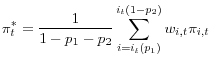
The ability of the core measures to track trend inflation can be quantified by the root mean square error of the core inflation measure from trend inflation. It is unclear, however, how to treat a long-standing bias in the core measure when constructing goodness-of-fit measures, such as when a core measure persistently has an inflation rate 1 percentage point lower than overall inflation. Using the root mean square error to measure fit would always penalize for bias even though relatively constant and predictable bias between the core inflation indicator and overall inflation would only require the user to add an adjustment factor. On the other hand, using the standard deviation of the difference between the core measure and trend inflation would correct for the average bias over the time period, even if that bias were not predictable at the time.

This note takes an intermediate approach by assuming that users of the core inflation measure can adjust for bias by looking at the average difference between overall inflation and core inflation over the preceding 10 years. Thus in this note the ability of the core measure to track a measure of trend inflation is given by the root mean square error adjusted for expected bias:

$\displaystyle tracking error\equiv \sqrt{mean({({\pi }^{core}_{t,t-s}-{\pi }^{trend}_t-{{\frac{\sum^{t-1}_{m=t-121}{({\pi }^{core}_{m,m-s}-{\pi }^{trend}_m)}}{120}}})}^2)}$

(1)

where ${\pi }^{trend}_t$ denotes the trend inflation rate at time t, and ${\pi }^{core}_{t,t-s}$ denotes the inflation rate in the core measure between time t and t-s (defined as ${{{\frac{{\rm 1200}}{{\rm s}}{\rm *}}}\ln \left({{\frac{{price level}_t}{{price level}_{t-s}}}}\right) }$ ).¹⁰ For most core measures the qualitative results would be unchanged if either of the other two approaches of treating bias were followed.¹¹

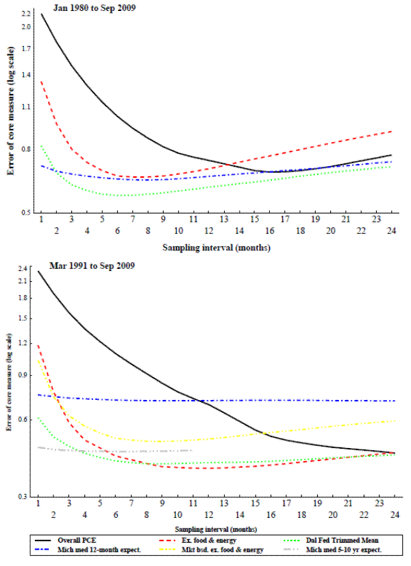
Figure 1 displays the standard error of some prominent core inflation indexes using a centered 36-month moving average of headline PCE inflation as trend inflation, Figure 2 shows the same data, but uses a Baxter-King band pass filter to measure trend inflation.¹² The vertical axes in the figures use a logarithmic scale to emphasize the percentage, rather than the absolute, differences in fit across the core inflation indexes. The horizontal axis in each panel lists the number of months used in constructing the core measure's inflation rate (i.e., the sampling interval, s in formula 1). The two panels of each figure cover the time periods starting in 1980 and in 1991, with the core inflation measures being constructed through the summer of 2009, which is the most recent data available while still allowing enough additional data points to construct relatively reliable benchmarks for the comparison.¹³

Figures 1 and 2 show that of these common measures, the trimmed mean (the dotted line) performs generally better than the other measures at tracking trend inflation over most intervals, but the preference for that measure diminishes as the interval lengthens out. In the more recent time period (the bottom panel) there is little difference between the trimmed mean and prices excluding food and energy once the interval is around 9 months or longer. Overall inflation also performs quite well with the Baxter-King filter in the longer time period when the interval is around twelve months, but it performs less well at short intervals and when the 36-month moving average is used as to measure trend inflation. The performance of survey measures of inflation expectations, unlike the indexes constructed actual price data, do not improve much with intervals over a few months. Finally, the best interval for almost all of the measures tends to be longer in the more recent period, starting in 1991, than in the full sample, starting in 1980. This is likely a result of inflation in the past 20 years having been low with very little long-run trend.

Test 2: Predicting future inflation

The ability of the core inflation measure to predict future inflation is tested in the same way as the ability of the measures to track trend inflation. The only difference is the benchmark is now future inflation rather than trend inflation.¹⁴ Two different measures of future inflation are tested: overall inflation during the next twelve months, and overall inflation in the second half of the next 24 months (i.e. inflation 12 to 24 months ahead). Forecast horizons shorter than 12-months are not examined as those horizons would promote core measures that are good at predicting the transitory movements that core inflation measures are intended to filter out.

Results for the core measures ability to predict future inflation at these two horizons are shown in the two panels of figure 3 and of figure 4. They are similar to the results for the core measures ability to track trend inflation, though overall inflation performs somewhat worse relative to the other core measures, particularly in the longer period. Michigan median inflation expectations for the next twelve months perform fairly well at predicting future inflation in the longer period, but not so well in the more recent period. On the other hand Michigan median inflation expectations for the next five to ten years predict inflation very well in the more recent period, but data is not available far enough back to evaluate it over the longer period. As before overall PCE tends to require longer sampling intervals than the alternative inflation measures.

Test 3: Predicting inflation in a Phillips curve regression

A more general test of the forecasting ability of alternative core inflation measures runs a regression which includes some variables to explicitly account for movements in underlying inflation:

$\displaystyle {\pi }_{t+12,t}=\alpha +\beta {\pi }^{core}_{t,t-s}+\theta X_t+{\varepsilon }_t$

This test broadens the framework used in the second test by allowing $\beta$ to take on values different from 1, and allowing for the additional right-hand side variables, X. These changes create a simplified version of the expectations-augmented Phillips curve often used in inflation forecasting, with expected inflation equal to $\beta {\pi }^{core}_{t,t-s}$ . For this note the X variables added to the regression are the unemployment rate gap and share-weighted non-fuel import and oil price changes, as well as their lagged prices changes¹⁵:

$\displaystyle \theta X_t{\rm =}{\gamma }_{{\rm 1}}\left({unemployment{\rm }rate}_{t{\rm +}12,t}{\rm -}{nairu}_{t{\rm +}12,t}\right){+ \gamma }_{{\rm 2}}\left({unemployment{\rm }rate}_{t,t-12}{\rm -}{nairu}_{t,t-12}\right){\rm +}{\gamma }_{{\rm 3}}\left(w^{energy}_{t{\rm +}12,t}{\pi }^{oil}_{t{\rm +}12,t}\right){\rm +}{\gamma }_{{\rm 4}}\left(w^{energy}_{t,t{\rm -}12}{\pi }^{oil}_{t,t{\rm -}12}\right){\rm +}{\gamma }_{{\rm 5}}\left(w^{imports}_{t{\rm +}12,t}{\pi }^{imports}_{t{\rm +}12,t}\right){\rm +}{\gamma }_{{\rm 6}}\left(w^{imports}_{t,t{\rm -}12}{\pi }^{imports}_{t,t{\rm -}12}\right)$

A series of regressions using rolling ten-year windows, with starting and ending dates incremented one month at a time, are run to create out-of-sample forecasts for inflation over the next twelve-months. The first time period is shortened to begin at the start of 1985 to allow for enough data to obtain coefficient estimates.¹⁶

Results for this out-of-sample Phillips curve test are shown in figure 5. The errors in this figure are noticeably smaller than the comparable errors in the previous test, shown on figure 3, which do not include the additional right hand side Phillips curve variables. Since out-of-sample forecasts are used here, the reduction in errors is not simply a result of adding variables to improve regression fit. However, they are based on future values of the unemployment rate, oil prices, and import prices. These variables, while they cause changes in overall inflation, would not be available in real-time to a forecaster.

Figure 5 suggests that longer sampling intervals for the core measures are strongly preferred in Phillips curves. A long sampling interval is consistent with the usual practice of including multiple lags of inflation among the exogenous variables in a Phillips curve. Among the different measures shown in this figure the overall PCE inflation, PCE inflation excluding food and energy, and the Dallas Fed trimmed mean all perform roughly similarly. Michigan median 12-month inflation expectations, however, perform poorly over the longer sampling intervals.

Combining results from different tests and time periods

A next step is to combine the different tests and time periods to find a core measure at an interval which performs generally well over the many uses of a core inflation measure. While these combined results are dependent on the weights given to the various benchmarks and time periods they should still give a rough idea of which core measures work well and which do not.

The combination is created by taking geometric average of the error of the inflation measure under 15 different specifications, where the errors were defined earlier. The specifications comprise the 5 benchmarks from figures 1 through 5 (a centered 36-month moving average of overall inflation, a Baxter-King band-pass filtered version of overall inflation, overall inflation over the next 12 months, overall inflation in the 12 months following the next 12 months, and a Phillips curve for overall inflation in the next 12 months), and three time periods (January 1980 to September 2009¹⁷, March 1991 to September 2009, and January 2000 to September 2009).

The choice of time periods results in performance since 2000 being weighted more heavily than earlier performance. Such a weighting is appropriate if there have been structural changes in inflation data. One reason to think that there have been such changes is the continual updating of the methodology and structure for the CPI data which underlie most of the PCE prices series. For example, the third time period was chosen to correspond with the period following the major CPI revision in 1999.

Figures 6 through 9 display the average performance over the 15 specifications for the core inflation measures listed in table 1. As before, a logarithmic vertical axis is used to emphasis differences across the measures. For comparison across the types of core measures figure 10 takes some of the best performing measures from each type and displays them on a non-logarithmic axis.

Figure 6 displays the results for overall PCE inflation and various exclusion methods.¹⁸ Overall PCE performs by far the worst of the various measures at short sampling intervals. The performance of overall PCE inflation improves significantly as it is averaged over periods up to about 18 months. At that point its standard error is still above that of all of the exclusion indexes; however, the difference is relatively small. The exclusion indexes, except for including only services, all perform rather similarly and the performance of all of them improves until the interval reaches around 9 months.

The trimming-based measures, figure 7, do much better than exclusion indexes at short sampling intervals, but still improve with averaging the inflation rate up to about 7 or 8 months. All the trimmed measures perform similarly, with a very slight preference for the Dallas Fed trimmed mean.

Also on figure 7 are the Michigan 12-month-ahead inflation expectations measures. Other expectations measures do not go far enough back to be included in this round-up. These measures perform well at the one-month interval, but do not improve much with longer sampling intervals. By the nine-month interval the expectations measures perform notably worse than the trimmed measures. Median inflation expectations perform better than mean expectations.

Figure 8 shows the results from methods that recombine the current inflation rates of the various components using other weighting schemes. In variance weighting, components with more variable relative prices or inflation rates receive a correspondingly lower weight. In many ways this idea is a more refined version of the trim- and exclusion- based measures depending on how the variance is calculated. Here the variance is calculated from relatively recent price changes, so the variance of an item is allowed to change over time. This makes the variance-weighted indexes more similar to the trim-based measures than to exclusion indexes, and many of the variance weighted measures perform similarly to the trimmed-based measures. Results for two of these variance-weighted measures tested are shown in figure 8. Using the variance of price changes to set the item weight tends to work slightly better than using the variance of the relative price level or the variance of the change in the price change, but the results are not dramatically different. (For space reasons, only one of these additional permutations is shown.) Also on figure 8 are the results from Eusepi, et al's cost of nominal distortions price index (CONDI), which essentially gives greater weight to items who frequency of price change is lower (among other factors). This index performs similarly many of the exclusion-based price indexes. The final type of measures shown in figure 8 use component weights from a regression of the disaggregated components on overall PCE inflation. These regression-based models do not to fit terribly well, and lengthening the interval had little effect on their performance.

Among the techniques that are based on smoothing inflation over time, shown on figure 9, the results from a couple low-order ARIMAs using rolling 15-year windows perform well. The other smoothing techniques also perform decently, but not as good as the ARIMAs. Component smoothed inflation and exponentially smoothed inflation performed slightly worse than the UC-SV measure. It is notable, though not surprising, that the smoothing methods, other than the ARIMA(2,0,1), do not require a long interval. Presumably this is because they are already averaged over time.

Figure 10 displays some of the best performing measures in each category, along with overall PCE and an average of the three most common PCE inflation measures (overall PCE, prices excluding food and energy, the Dallas Fed trimmed mean). As noted above the best interval for overall PCE inflation seems to be at least 18 months, and the average error keeps falling slightly through 20 months.

On average across all the intervals, excluding food and energy performs somewhat worse than the potential other indexes, and overall PCE performs considerably worse than any of the measures including excluding food and energy. This suggests that core inflation measures are useful and there may be better measures of core inflation than excluding food and energy.

One the other hand, when each measure is examined at its best interval the difference across measures is much less pronounced. Overall PCE inflation still performs the worst, then excluding food and energy performs next worst, and the other measures perform better than these two measures, but the difference is small. The error from using excluding food and energy at its best interval (0.79 at an interval of 13 months) is only slightly higher than the error when using the best measure, the Dallas Fed trimmed mean at its best interval (0.77 at an interval of 15 months), and only slightly lower than using overall PCE inflation at its best interval (0.82 at an interval of 20 months). Assessing whether the differences across measures are statistically significant in a formal test would be difficult since the 15 different specifications are not independent.¹⁹

Also as can be seen on figure 10 combining inflation measures only leads to a small improvement. The averaging of overall inflation, excluding food and energy, and the trimmed mean performs only a couple basis point better at most intervals than simply using the trimmed mean. The small improvement when averaging suggests that the measures tend to make similar errors when tracking underlying inflation or predicting future inflation.

Are the core measures useful in other time periods?

As noted in the introduction, a core measure is only useful if it can perform the goals of tracking current trend inflation or predicting future overall inflation better than overall inflation itself over a significant period of time. The results above show that this may be the case, but they could merely be the result of the aggregation placing a large amount of weight on the post-2000 time period. To demonstrate that this is not the case, figures 11 through 14 take most of the measures from figure 10 and display how they fit a geometric average of the 5 benchmarks over rolling 10-year windows using a interval of 3 months (figure 11), 6 months (figure 12), 12 months (figure 13), or each index's best interval from the previous section (figure 14). One substitution is made from figure 10: the Dallas Fed trimmed mean is replaced by the average trimmed mean because the Dallas Fed does not publish their measure prior to 1977. Over the period where both trimmed mean measures are available they perform quite similarly.

Over this longer sample, the trimmed mean, the variance weighted, and the average of overall PCE, PCE excluding food and energy, and the trimmed mean all perform similarly regardless of the interval used. These three measures generally perform notably better than excluding food and energy or overall PCE prices at sampling intervals of 6 months or less. At a twelve month interval there some periods where overall PCE inflation performs the best, while at each index's best interval the differences across measures is relatively small and swamped by the difference in performance of all the measures across time.

Conclusion

There is no universally "best" core inflation measures, just as prior studies have found. Nonetheless, a number of conclusions can still be drawn from the results here:

First, short sampling intervals should be avoided. Almost all the inflation measures, except survey-based measures and already smoothed indexes, must be averaged over a significant time interval to best track underlying inflation or predict future inflation. The best interval depends on the measure and the time period, but at present for overall PCE inflation sampling intervals shorter than 18 months should be avoided. For other measures of PCE prices inflation the best sampling intervals in the tests here were often around 12 months.

Second, at sampling intervals of 12 months or less since the mid-1980s overall PCE inflation performs worse at predicting future inflation or matching ex-post measures of trend inflation than many other core measures including excluding food and energy, variance weighted inflation, or the Dallas Fed trimmed mean. Even when each measure is evaluated at its best interval, overall PCE inflation still performs slightly worse than the majority of potential core measures, though the difference may not be statistically or economically significant.

Third, trimmed mean or variance weighted price indexes perform slightly better than exclusion indexes such as PCE prices excluding food and energy, particularly at short intervals. Though, again, the difference between measures when each is evaluated at its best interval may not be statistically or economically significant. However, it does suggests that if we desire a single real-time measure of core inflation there may be better choices than simply excluding food and energy.

Appendix: Description of the core inflation measures

This appendix gives an overview of some of the core inflation measures examined in this note.

Exclusion Indexes

Inflation indexes resulting from removing certain items throughout history are referred to as exclusion indexes. To account for the removed items, the weights of the items remaining in the index are scaled up and their relative weights are unaffected. Exclusion indexes are the most popular measures of core inflation for their simplicity and transparency: They are easily constructible in real time, communicable to the public, and replicable with published inflation data. Clark (2001) prefers CPI prices excluding energy in his overview of core inflation measures.

One variant of deciding what items should be excluded is to include only "sticky" prices (Aoki 2001). Following a similar procedure to that used by Bryan and Meyer (2010) for the US CPI, a sticky price index for this note is created by examining a list of the frequency of price changes from Bils and Klenow (2004) and excluding the 30 percent of the consumption basket with the most frequent price changes.

Statistical Central Tendency Measures

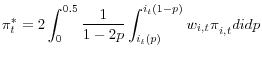
When the cross-sectional distribution of price change has fat tails, the mean may be very sensitive to outliers. As a result, Bryan and Pike (1991) and Bryan and Cecchetti (1994) advocated the use of weighted medians and trimmed means to measure underlying inflation. These indexes exclude different items each month depending on their place in the cross-sectional distribution of price changes. The monthly price change for the index is determined by ordering the items by their price change over the month, from most negative to most positive, and then removing the components in the tails of the distribution up to a certain share of the consumption basket. The price change is then computed from the remaining items. The basic formula for these types of measures is:

$\displaystyle {\pi }^*_t={{\frac{1}{1-p_1-p_2}\sum^{i_t\left(1-p_2\right)}_{i=i_t\left(p_1\right)}{w_{i,t}{\pi }_{i,t}}}}$

where $\pi$ ${}_{i,t}$ is the inflation rate of the i ${}^{th}$ item in the ordered cross sectional inflation distribution, $\rho$ ${}_{1}$ is trim on the lower side, $\rho$ ${}_{2}$ is the trim on the upper side, $i_t\left(p\right)$ is the item at the p-point in the cross sectional inflation distribution at time t, $w_{i,t}$ is the weight of item i in the consumption basket at time t, and ${\pi }_{i,t}$ is the inflation rate of item i in month t. Twelve-month changes are constructed as the cumulation of the one-month changes.

Dolmas (2005) created a version of the trimmed mean for the PCE price index, which is published monthly by the Dallas Federal Reserve Bank. Dolmas' version is not symmetric; it uses $\rho$ ${}_{1}$ =.194, $\rho$ ${}_{2}$ =.254. Thus, the measure excludes 44.8 percent of the consumption basket. In the weighted median $\rho$ ${}_{1}$ = $\rho$ ${}_{2}$ =.5, so only the inflation rate of the item at the very middle of the cross-sectional distribution is used. Smith (2004) finds this index performs quite well.

The trimmed mean requires the designer to determine cut-off points. For the Dallas Fed trimmed mean the cut-off points were designed so that the measure would best fit benchmarks over the years 1977 to 2004. To avoid possible contamination from the cut-off points being determined ex-post, an alternative version that averages across all possible symmetric trims from no trim ( $\rho$ ${}_{1}$ = $\rho$ ${}_{2}$ =0) to the largest possible trim ( $\rho$ ${}_{1}$ = $\rho$ ${}_{2}$ =.5) was constructed for this paper. This average trimmed mean takes a more agnostic view of the appropriate cut-off points. In contrast to the normal trimmed mean or weighted median, this formulation does not completely ignore the information in the tails, but instead down-weights those observations. The formula for this type of measure is:

$\displaystyle {\pi }^*_t=2\int^{0.5}_0{{{\frac{1}{1-2p}\int^{i_t\left(1-p\right)}_{i_t\left(p\right)}{{w_{i,t}\pi }_{i,t} di dp}}}}$

The average trimmed mean measure performs quite similarly to the normal trimmed mean produced by the Dallas Fed except for being somewhat more biased. ${}^{ }$ ²⁰

The trimmed measures used here all trim based on the one-month price changes. However, there is no reason that longer sampling intervals, such as price changes over three or twelve month periods, could not be used to determine which items to trim.

Trimmed mean of volatile components

The trimmed mean of volatile components (TMVC) proposed in Pedersen (2009) combines aspects of the trimmed mean approach and the exclusion index approach. The TMVC removes a fixed share of the consumption basket each month based on the volatility of the inflation rate of the item. Like the other central tendency measures, items are ranked according to certain criteria and a fixed percentage of the consumption basket is removed, the items removed each month may vary, and information on inflation from the current month is used in constructing the ranking. Like the exclusion index approach, the history of the items does matter. Pedersen ranks CPI components by the variance of their monthly inflation rates over the past 6 to 24 months and then removes the most volatile components. He finds the best indexes for the placecountry-regionUnited States exclude between 3 and 47 percent of the consumption basket. The TMVC specification used in this paper removes the most volatile 25 percent of the consumption basket based on monthly inflation over the prior 24 months (including the most recent observation). The same 205-component disaggregation of overall PCE as used in the average trimmed mean is used to construct the TMVC.

Variance-weighted (Neo-Edgeworth Indexes)

Instead of completely removing volatile components, a neo-Edgeworth index down-weights the volatile components (Diewert 1995). Often each item is weighted by the inverse of its variance. In fact, if each component had equal shares in the consumption basket, there were no long-run relative price changes across the components, and shocks to a component's price change were not correlated across components or across time, then weighting each item by the inverse of that item's variance would be optimal. However, these restrictions are not observed in practice.

Variance-weighted price indexes may give a lot of weight to items that have a low variance but make up a small share of the consumption bundle. To reduce this problem, rather than strictly using the inverse of the monthly variance of the item's price change to weight the item, the inverse of 1 plus the monthly variance of the item's price change is multiplied by the item's nominal share. These weights are normalized to sum to one across all items. The variance of the monthly percentage change in price for each component is taken over backward-looking 60-month windows.

The same 205-component disaggregation of PCE prices used for constructing a number of the other core measures was used to construct the variance-weighted indexes.

A large number of additional formulations of variance-weighted inflation were also tested. The formulations differed by what variance was constructed and by the weight given to past observations in constructing that variance. First, beyond just taking the variance of the one-month price change of the component, three additional variances were constructed: 1. The variance of the one-month price change of the component relative to the one-month price change of overall PCE, 2. The variance of the component price level relative to the price level of overall PCE, and 3. The variance of the change in the monthly inflation rate (i.e. the second moment of the price level). As before these were multiplied by the items nominal share.

Further formulations were constructed by changing the treatment of older observations for each of these three variance measures. Older observations were down-weighting when constructing the variance in geometrically-declining fashion. Monthly discount rates ranging from 0.05 percent (very slowly declining weights on past observations) to 50 percent (very little weight on past observations) were evaluated.

In nearly all cases the different permutations had only a small effect on the results, leaving the majority of variance weighted measures to perform similarly.

Smoothed versions of headline inflation

The indexes above all rely on looking at the disaggregated components. On the other hand much work has been done simply focusing on ways of pulling a trend out of the headline inflation and eschewing any information in the components.

Cogley (2002) suggests exponentially smoothing headline inflation. This method sets the core inflation rate to a long moving average of past inflation: ${\pi }^*_t=\alpha \sum^{\infty }_0{{\left(1-\alpha \right)}^j{\pi }_{t-j}}$ . This can also be written as core inflation equals weighted average of current inflation and lagged core inflation, ${\pi }^*_t=\alpha {\pi }_t+\left(1-\alpha \right){\pi }^*_{t-1}$ , or as an IMA(1,1) process, ${\pi }_{t+1}-{\pi }_t={\varepsilon }_{t+1}-{\left(1-\alpha \right)\varepsilon }_t$ where ${\pi }^*_t= E_t\left({\pi }_{t+1}\right)={\pi }_{t+1}-{\varepsilon }_{t+1}$ . Cogley suggests setting $\alpha$ equal to .875 for quarterly CPI inflation (i.e. a 12.5 percent quarterly discount rate).

Stock and Watson (2008) suggest what amounts to a generalization of Cogley's procedure that allows the moving average term in the IMA(1,1) to vary over time following an approximate logarithmic random walk. ${}^{ }$ ²¹ They find that their unobserved components-stochastic volatility (UC-SV) model fits quarterly inflation quite well, and it out-performs traditional Phillips curves since 1985.

They suggest that the projection from an IMA(1,1) using rolling 10-year windows performs only slightly worse than their UC-SV model. Similarly, for the monthly data used in this paper rolling 15-year windows of many ARIMAs with at least one MA term, at least one autoregressive or degree of integration, but no more than 1 degree of integration, perform quite well.

Component Smoothed Inflation

Rather than throwing away the underlying component data and simply smoothing headline inflation, Gillitzer and Simon (2006) suggest smoothing individual components by a degree appropriate for that item and then aggregating these smoothed components. This concept has a couple of advantages: First, the concept is easily grasped by the lay person: certain items are volatile, therefore these items need to be smoothed more than other items. Second, each item receives its normal weight in the consumption basket. This makes the index relatively immune to both the populist complaint that "the central bank throws out the items which are increasing when looking at inflation", and problems associated with diverging trend inflation rates across components, which can cause the index to be biased one way or the other.

Component smoothing has not been widely explored, and there are many potential alternative methods for smoothing the components that might improve the technique but have not yet been examined. These possible methods include using a simple average of the component over the prior x-months, applying Stock-Watson's UC-SV model to each item, or allowing changes in the degree of smoothing to be correlated across items. The technique used for smoothing in this paper differs from Gillitzer and Simon. Here the degree of smoothing is determined for each item by a single exponential smoother calibrated to predict the item's twelve-month-ahead inflation rate over the previous ten years. The smoothing component varies across the items from .01 to .16 with a median value of .07, which implies the median item is smoothed with a mean lag of 14 months.

The level of component disaggregation is likely to be important for the fit of a component smoothed index. This uses the same 205-component disaggregation of PCE to construct component smoothed inflation that was used to construct the weighted median, the TMVC, and variance-weighted inflation.

Regression weights

Smith (2007) suggests that the forecast from a regression of headline inflation on the lagged disaggregated components of inflation provides a good measure of core inflation. Specifically, the basic regression form is:

$\displaystyle {\pi }_{t,t-12}=c+{\theta }_1{\pi }_{1,t-12,t-24}+{\theta }_2{\pi }_{2,t-12,t-24}+{\theta }_3{\pi }_{3,t-12,t-24}+{\theta }_4{\pi }_{4,t-12,t-24}+\dots +{\varepsilon }_t{\rm }{\rm }$

, where ${\pi }_{t,t-12}$ is headline inflation rate over the past twelve months, and ${\pi }_{i,t-12,t-24}$ is the inflation rate of the i ${}^{th}$ component over the twelve months prior to the past twelve months. Using the coefficients from this regression a forecast for headline inflation over the next twelve months, ${\pi }_{t+12,t}$ is constructed and considered the estimate of core inflation at time t.

Following Smith's basic methodology 48 regression-based variants were constructed. Most of these results are not shown for space reasons. The variants differed according to:

1. The degree of disaggregation: Both a 17-component disaggregation of PCE prices based on NIPA table 2.3.4 and 51-component disaggregation suggested by Smith were used. The 17-component disaggregation performed somewhat better than the 51-item disaggregation.

2. Whether the inflation rates of the components were multiplied by their share in the consumption basket in the regression. This allows the contribution of an item's inflation to headline inflation to evolve as expenditure patterns change over time. This multiplication did improve the results slightly.

3. Whether the observations were equally weighted (with a start date of 1972) or instead older observations were down-weighted in a geometrically declining fashion (with a start date of 1959). One fixed weighted and eleven geometrically declining permutations, with discount rates of 0.05 percent to 5 percent per month, were constructed. There was no clear preference for either discounting or fixed weighting.

Additional variants, such as restricting the regression constant to zero, the sum of the coefficients to 1, and the coefficients to be non-negative, were not examined.

References

Ang, Andrew, Geert Bekaert, and Min Wei (2007),

"Do Macro Variables, Asset Markets, Or Surveys Forecast Inflation Better?" Journal of Monetary Economics vol. 54, no. 4, pp. 1163-1212.

Aoki, Kosuke (2001), "Optimal Monetary Policy Responses to Relative-Price Changes," Journal of Monetary Economics, vol. 48, no. 1, pp. 55-80.

Arrazola, Maria, and Jose de Hevia (2002), "An Alternative Measure of Core Inflation," Economics Letters, vol. 75, no. 1, pp. 69-73.

Bagliano, Fabio C., and Claudio Morana (2003), "Measuring US Core Inflation: A Common Trends Approach," Journal of Macroeconomics, vol. 25, no. 2, pp. 197-212.

Bilke, Laurent, and Livio Stracca (2007), "A Persistence-Weighted Measure of Core Inflation in the Euro Area," Economic Modelling, vol. 24, no. 6, pp. 1032-1047.

Bils, Mark, and Peter J. Klenow (2004), "Some Evidence on the Importance of Sticky Prices," Journal of Political Economy, vol. 112, no. 5, pp. 947-985.

Blinder, Alan, and Ricard Reis (2005), "Understanding the Greenspan Standard," The Greenspan Era: Lessons for the Future, A symposium sponsored by the Federal Reserve Bank of Kansas City, Jackson Hole, Wyoming, August 25-27, 2005.

Brischetto, Andrea, and Anthony Richards (2007), "The Performance of Trimmed Mean Measures of Underlying Inflation," RBA Research Discussion Paper 2006-10: Revised, Reserve Bank of Australia. Presented at Federal Reserve Bank of Dallas, Conference on Price Measurement for Monetary Policy, May 24-25, 2007.

Bryan, Michael F., and Brent Meyer (2010), "Are Some Prices in the CPI More Forward Looking than Others? We Think So," Economic Commentary, Federal Reserve Bank of Cleveland, May 19.

Bryan, Michael F., and Brent Meyer (2011), "Should We Even Read the Monthly Inflation Report? Maybe not. Then again...," Atlanta Fed Macroblog June 1, 2011.

Bryan, Michael F., and Christopher Pike (1991), "Median Price Changes: An Alternative Approach to Measuring Current Monetary Inflation," Economic Commentary.

Bryan, Michael F., and Stephen G. Cecchetti (1994), "Measuring Core Inflation," in Mankiw, N. G. ed., Monetary Policy. Studies in Business Cycles, vol. 29; Chicago and London:; University of Chicago Press, pp. 195-215.

Catte, Pietro, and Torsten Slok (2005), "Assessing the Value of Indicators of Underlying Inflation for Monetary Policy," OECD Economics Department Working Papers:461.

Cecchetti, Stephen G. (1997), "Measuring Short-Run Inflation for Central Bankers," Federal Reserve Bank of St. Louis Review, vol. 79, no. 3, pp. 143-155.

Clark, Todd E. (2001), "Comparing Measures of Core Inflation," Federal Reserve Bank of Kansas City Economic Review, vol.86, no. 2, pp. 5-31.

Clinton, Kevin (2006), "Core Inflation at the Bank of Canada: A Critique,"Queen's University Department of Economics Working Paper 1077.

Cogley, Timothy (2002), "A Simple Adaptive Measure of Core Inflation," Journal of Money, Credit, and Banking, vol. 34, no. 1, pp. 94-113.

Crone, Theodore, N. Neil K. Khettry, Loretta J. Mester, and Jason A. Novak (2011), "Core Measures of Inflation as Predictors of Total Inflation,"Federal Reserve Bank of Philadelphia Research Department Working Paper No. 11-24. June.

Cutler, Joanne (2001), "Core Inflation in the UK," Bank of England, External MPC Unit Discussion Papers, No. 3.

Diewert, W. E. (1995), "On the Stochastic Approach to Index Numbers," University of British Columbia, UBC Departmental Archives.

Dolmas, Jim, and Mark A. Wynne (2008), "Measuring Core Inflation: Notes from a 2007 Dallas Fed Conference," Staff Papers, Federal Reserve Bank of Dallas, no. 4.

Dolmas, Jim (2005), "Trimmed Mean PCE Inflation," Federal Reserve Bank of Dallas, Working Papers: 05-06, pp. 1-29.

Domenech, Rafael, and Victor Gomez (2006), "Estimating Potential Output, Core Inflation, and the NAIRU as Latent Variables," Journal of Business and Economic Statistics, vol. 24, no. 3, pp. 354-365.

Eckstein, Otto (1981), Core Inflation. Englewood Cliffs, NJ: Prentice-Hall.

Eusepi, Stefano, Bart Hobjin, and Andrea Tambalotti (2011), "CONDI: A Cost of Nominal Distortions Index," American Economic Journal: Macroeconomics Vol 3, July. pp 53-91.

Folkertsma, C. K., and K. Hubrich (2001), "Performance of Core Inflation Measures," De Economist, vol. 149, no. 4, pp. 455-508.

Freeman, Donald G. (1998), "Do Core Inflation Measures Help Forecast Inflation?", Economic Letters, vol. 58, no. 2, pp. 143-147.

Giannone, Domenico, and Troy Matheson (2007), "A New Core Inflation Indicator for New Zealand," C.E.P.R. Discussion Papers 6469.

Gillitzer, Christian, and John Simon (2006), "Component-Smoothed Inflation: Estimating the Persistent Component of Inflation in Real Time," Reserve Bank of Australia, RBA Research Discussion Papers.

Kapetanios, George (2004), "A Note on Modelling Core Inflation for the UK using a New Dynamic Factor Estimation Method and a Large Disaggregated Price Index Dataset," Economic Letters, vol. 85, no. 1, pp. 63-69.

Meyer, Brent H., and Mehmet Pasaogullari (2010), "Simple Ways to Forecast Inflation: What Works Best?", Economic Commentary, Federal Reserve Bank of Cleveland, December 6.

Pedersen, Michael (2009), "An Alternative Core Inflation Measure," German Economic Review vol. 10, no. 2, pp. 139-164.

Quah, Danny, and Shaun P. Vahey (1995), "Measuring Core Inflation?" Economic Journal vol. 105, no. 432, pp. 1130-1144.

Reis, Ricardo, and Mark W. Watson (2007),"Relative Goods' Prices and Pure Inflation," NBER Working Paper, no 13615.

Rich, Robert, and Charles Steindel (2007), "A Comparison of Measures of Core Inflation," FRBNY Economic Policy Review, December.

Robalo Marques, Carlos, Pedro Duarte Neves, and Luis Morais Sarmento (2003), "Evaluating Core Inflation Indicators," Economic Modelling, vol. 20, no. 4, pp. 765-775.

Rowe, Nick (2011), "No, Atlanta and St. Louis Fed, you can't test whether core is useful that way," A Worthwhile Canadian Initiative: Blog post of June 2, 2011.

Silver, Mick (2007), "Core Inflation: Measurement and Statistical Issues in Choosing among Alternative Measures," IMF Staff Papers, vol. 54, no. 1, pp. 163-190.

Smith, Julie K. (2007), "Better Measures of Core Inflation," Presented at Conference on Price Measurement for Monetary Policy, Federal Reserve Bank of Dallas, May 24-25, 2007.

Smith, Julie K. (2004), "Weighted Median Inflation: Is this Core Inflation?" Journal of Money, Credit, and Banking, vol. 36, no. 2, pp. 253-263.

Stock, James H., and Mark W. Watson (2008), "Phillips Curve Inflation Forecasts," NBER Working Paper, no. 14322.

Velde, Francois R. (2006), "An Alternative Measure of Inflation," Federal Reserve Bank of Chicago Economic Perspectives, vol. 30, no. 1, pp. 55-65.

Wynne, Mark A. (2008), "Core Inflation: A Review of some Conceptual Issues," Federal Reserve Bank of St. Loius Review, vol. 90, no. 3, part 2, pp. 205.

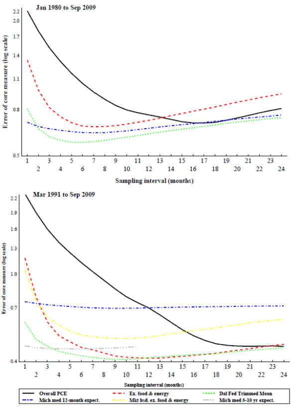
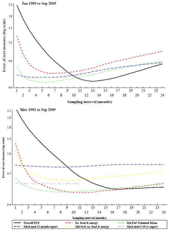
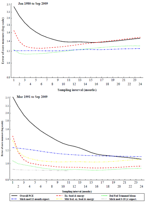
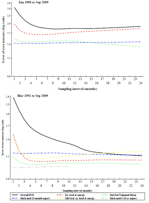
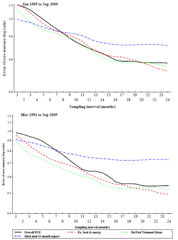
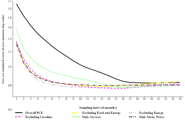
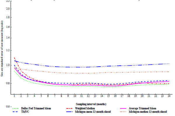
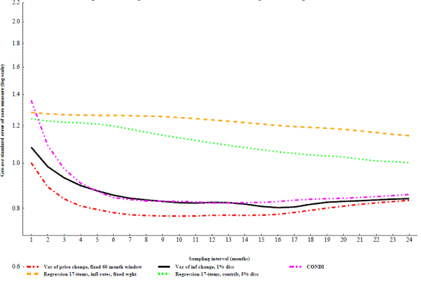
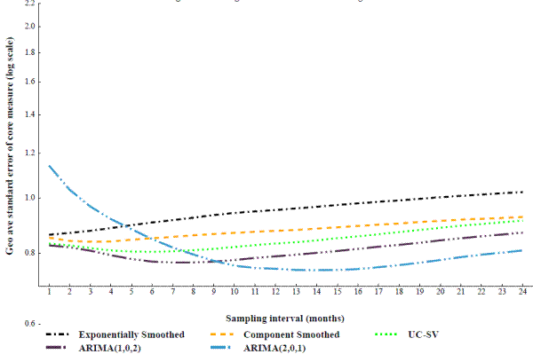
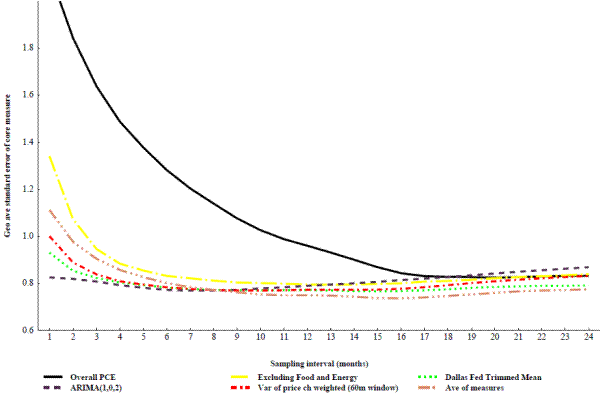
Figure 11: Average Performance of Selected Core Inflation Measures at 3-month Sampling Interval.

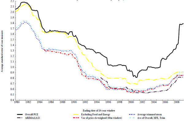Figure 11 Data

Figure 12: Average Performance of Selected Core Inflation Measures at 6-month Sampling Interval.

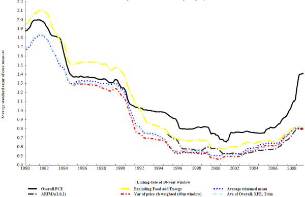Figure 12 Data

Figure 13: Average Performance of Selected Core Inflation Measures at 12-month Sampling Interval.

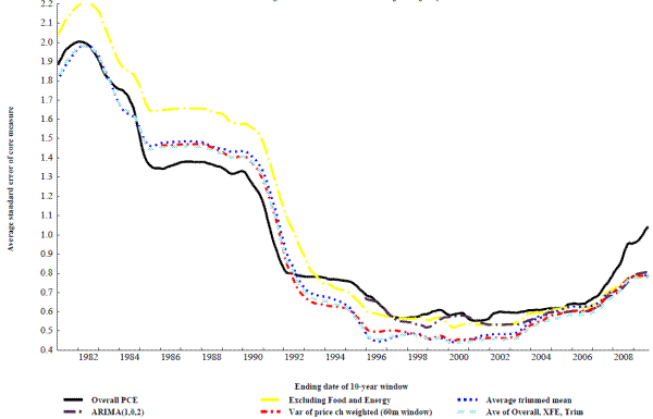Figure 13 Data

Figure 14: Average Performance of Selected Core Inflation Measures at Each Measure's Best Sampling Interval.

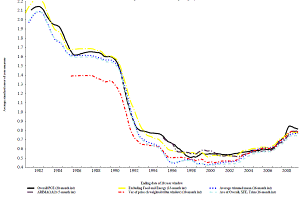Figure 14 Data

Figure A1: Tracking a Christiano-Fitzgerald band-pass filter of overall PCE inflation.

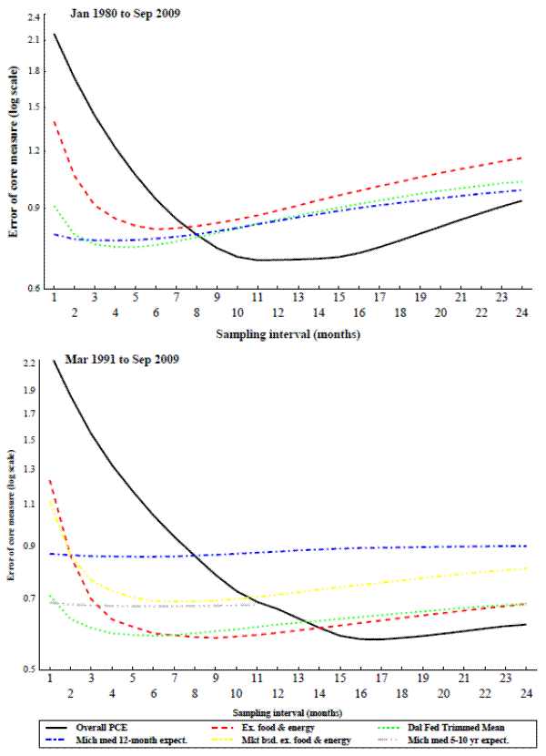Figure A1 Data

Figure A2: Tracking a Hodrick-Prescott filter of overall PCE inflation.

Figure A2 Data

Figure A3: Measures of Trend PCE Inflation.

Figure A3 Data

Footnotes

1. The views expressed herein are those of the author and do not necessarily reflect those of the Federal Reserve Board or its staff. For helpful comments and assistance I thank Monica Savukinas, Deb Lindner, David Lebow Dan Sichel, Peter Tulip, John Roberts, Michael Kiley, Julie Smith, Jim Dolmas, Joseph Chien, Robert Rich, Michael Pedersen, Mark Wynne, Bart Hobjin and numerous Federal Reserve Board staff. Return to Text

2. Email: [email protected] Return to Text

3. Other empirical comparisons of US core inflation measures include: Bryan and Cecchetti (1994), Cecchetti(1997). Freeman (1998), Clark (2001), Cogley (2002), Robalo Marques, et al. (2003), Smith (2004), Catte and Slok (2005), Brischetto and Richards (2007), Meyer and Pasaogullari (2010), and Crone et al. (2011). Return to Text

4. This definition of core inflation measures as including only actual price data is more restrictive than found in some places in the literature, and would exclude some measures that have been marketed as core measures, notably Eckstein's definition of core inflation as an average of unit labor costs and the cost of capital (Eckstein 1981), and Quah and Vaney's bivariate VAR of inflation and industrial production (Quah and Vahey 1995). However, this line is drawn to distinguish a concept of core inflation from more fully articulated inflation forecasts. For more on other aspects of the lack of definition in the core inflation literature see the report by Dolmas and Wynne on a 2007 core inflation conference (Dolmas and Wynne 2008). Return to Text

5. For example, the Bank of Canada's core price index excludes indirect taxes and eight of the most volatile components (fruit, fruit preparations and nuts, vegetables and vegetables preparations, mortgage interest costs, natural gas, fuel oil and other fuels, gasoline, inter-city transportation, and tobacco products and smokers' supplies), while the Bank of Japan uses an exclusion index that only removes fresh food. Return to Text

6. The choice of using the PCE price index, rather than the CPI, was driven by PCE item structure. When the BEA revises the PCE item structure the revision of categories is carried throughout the history of the index. In the CPI, such category changes are only done on a forward going basis. A uniform disaggregation of sub-headline price categories throughout the history of the price index greatly simplifies the construction the various alternative core inflation measures. Return to Text

7. Specifically, out-of-sample in this context means that the core inflation measure for a given date is constructed using only information from that date and previous dates. However, all measures are constructed and compared using an early-November 2011 vintage of data. Thus the tests are not "real-time" comparisons. The ex-post measures of trend inflation used to test the core measures against are not constructed on an out-of-sample basis, and use information from the full data sample. Return to Text

8. Other attributes that have been suggested for a core inflation measure include that the core inflation measure should not undergo large revisions, should not be affected by non-core inflation, should be highly correlated with money growth, and should be unbiased when compared to total inflation. Return to Text

9. These ex-post measures of trend inflation are not potential core inflation measures themselves, because they can not be reliably constructed in real time (i.e. they have end point problems). Return to Text

10. The bias adjustment is calculated over the available data when less than 10-years of data for the core measure is available. For survey-based inflation expectations ${\pi }^{core}_{t,t-s}$ is the average value reported between time periods

and

. This timing slightly handicaps the survey measures, because it does not take into account that survey data for month

is usually known before the actual PCE inflation data for month

is released. Return to Text

11. The most notable difference between the results which penalize for bias and those which do not is the performance of the survey-based measures, which would suffer considerably in the post-1991 period if bias were penalized. Another difference that would occur under either of the other two treatments of bias would be slightly stronger preference for the Dallas Fed Trimmed mean, though part of this could simply be the result of the trim points in the Dallas Fed measure being determined ex-post to fit data that largely overlaps with the data used here. Return to Text

12. Results using a couple of other common measures of trend inflation are similar and are shown in the appendix. Trend inflation is measured by a Christiano-Fitzgerald band-pass filter in appendix figure A1 and by a Hodrick-Prescott filter in appendix figure A2. Appendix figure A3 shows the path of the various measures of trend inflation along with actual inflation over the next 12 months. Return to Text

13. These time periods were chosen as the longest periods available that would include Michigan inflation expectations over the next 12 months (the period starting in 1980) and Michigan five-to-ten-year ahead inflation expectations (the period starting in 1991). To reduce endpoint problems with the filters the final 24 months (October 2009 to September 2011) are discarded. Similarly, in a later test, the comparison of the core inflation to inflation 24 months in the future, requires 24-months of data after the last period of the core inflation measures. Return to Text

14. The form of predicting future inflation used here differs slightly from other papers in the core inflation literature which tend to use a form of the regression ${\pi }_{t+12,t}=\alpha +\beta {\pi }^{core}_{t,t-s}+{\varepsilon }_t$ (Blinder and Reis (2005), and Crone, et al. (2011)) or ${\pi }_{t+12,t}- {\pi }_{t,t-s}=\alpha +\beta ({\pi }^{core}_{t,t-s}-{\pi }_{t,t-s})+{\varepsilon }_t$ (Clark (2001), Cogley (2002), Rich and Steindel (2007)). The form used in this paper differs by constraining the coefficient to 1 and constraining the constant to the average difference between total inflation and the core measure over the past ten years. These constraints are imposed to more accurately reflect the way a core inflation measure is likely to be used by non-inflation forecasters. (Inflation forecasters, other the other hand, are likely to use a more-fully specified model, perhaps something akin to the third test in this note.) More broadly, using core inflation measures to predict inflation has been criticized through a variant of the Lucas critique: if the central bank uses the core measure to predict inflation and the central bank is able to control inflation with only random error then the core measure should lose its ability to predict inflation and the best predictor of inflation should be the central bank's target (Clinton 2006, Rowe 2011). Since assumptions surrounding this critique are fairly strong (particularly since the FOMC does not release an inflation target), the critique is ignored here, as it is in most of the core inflation literature. Return to Text

15. The weights for energy prices, $w^{energy}_{t{\rm ,s}}$ , are final energy goods and services personal consumption expenditures as share of overall personal consumption expenditures. This serves as a proxy for the overall energy share in consumption input costs. The weights for imports, $w^{imports}_{t{\rm ,s}}$ , are nonpetroleum imports as a share of personal consumption expenditures. Return to Text

16. For the initial few years of the first time period the rolling window is shorter than ten years as the start data of the first window is set to 1979, to align with the start date of some of the core measures. The start date remains at 1979 until there is 10 years of data available. Return to Text

17. As in the previous section the first time period starts in January 1985 for the Phillips curve benchmark. Return to Text

18. Market-based PCE measures as constructed by the BEA does not extend far enough back for inclusion here. Return to Text

19. Crone, et al. (2011) find that the difference in errors between core measures and overall inflation is often not statistically significant, though their methodology differs from that here. Return to Text

20. To construct the average trimmed mean a 205-component breakdown of PCE prices, derived from BEA table 2.4.4U, is used. This breakdown is the most disaggregated possible from publicly available data in which every category contains monthly observations back to 1959. When a component in table 2.4.4U did not have data back to 1959, the lowest subaggregate with data back to 1959 was used instead of the individual component indexes comprising the subaggregate. A handful of items enter PCE with a negative weight. These items are treated the same as any other except that their weights are negative. This differs from Dolmas who removes components with negative weights before creating the trimmed mean PCE price index. Tests using an older vintage of data suggest that the inclusion or exclusion of these items has little effect on the resulting index. Return to Text

21. Specifically the UC-SV model can be written as an IMA(1,1) with a time-varying coefficient on the moving average component: ${\pi }_{t+1}-{\pi }_t={\varepsilon }_{t+1}-{{\theta }_t\varepsilon }_t$ . Since any moving average model can be rewritten as an autoregressive model with infinite lags, this model can be rewriting in its AR representation: ${\pi }_{t+1}=\left(1-{\theta }_t\right){\pi }_t+{\theta }_t\left(1-{\theta }_{t-1}\right){\pi }_{t-1}+{\theta }_t{\theta }_{t-1}\left(1-{\theta }_{t-2}\right){\pi }_{t-2}+{\theta }_t{\theta }_{t-1}{\theta }_{t-2}\left(1-{\theta }_{t-3}\right){\pi }_{t-3}+\dots +{\varepsilon }_{t+1}$ Increasing $\theta$ puts less weight on recent lags of inflation and more weight on older lags. Return to Text

^♣ This version is optimized for use by screen readers. Descriptions for all mathematical expressions are provided in LaTex format. A printable pdf version is available. Return to Text

The Usefulness of Core PCE Inflation Measures1

Introduction

References

Description of PCE Price Inflation Measures and Their Average Inflation Rates

Figure 1: Tracking centered 36-month moving average of overall PCE inflation.

Figure 2: Tracking a Baxter-King band-pass filter of overall PCE inflation.

Figure 3: Predicting inflation in the next twelve months.

Figure 4: Predicting inflation 12-to-24 months ahead.

Figure 5: Predicting inflation in the next 12 months using Phillips curve.

Figure 6: Average Performance of Exclusion Methods.

Figure 7: Average Performance of Trim Methods and Inflation Expectations.

Figure 8: Average Performance of Variance and Regression-Weighted Methods.

Figure 9: Average Performance of Smoothing Methods

Figure 10: Average Performance of Selected Core Inflation Measures.