Skip to: [Printable Version (PDF)] [Bibliography] [Footnotes]

Finance and Economics Discussion Series: 2012-13 Screen Reader version ^♣

The Relationship Between Information Asymmetry and Dividend Policy

Cindy M. Vojtech¹

March 2012

Keywords: Dividends, earnings management, information asymmetry, Sarbanes-Oxley act, financial disclosure

Abstract:

This paper examines how the quality of firm information disclosure affects shareholders' use of dividends to mitigate agency problems. Managerial compensation is linked to firm value. However, because the manager and shareholders are asymmetrically informed, the manager can manipulate the firm's accounting information to increase perceived firm value. Dividends can limit such practices by adding to the cost faced by a manager manipulating earnings. Empirical tests match model predictions. Dividend-paying firms show less evidence of earnings management. Furthermore, nondividend payers changed earnings announcement behavior more than dividend payers following the Sarbanes-Oxley Act, a law that increased financial disclosures.

JEL Classification: G30, G35, G38, K22, M41, M43

1 Introduction

The use of dividends is a common practice by U.S. public firms, totaling around $690 billion in 2010.² From a tax perspective, paying dividends is inefficient because managers can use the same cash to invest in firm growth, generating capital gains.³ This paper provides an explanation of dividend behavior by showing how dividend policy helps mitigate agency problems. Dividend policy limits a manager's discretion over accounting reports; dividends therefore make reported earnings more informative.

A manager of a public company makes many investment decisions that are not seen by shareholders. Shareholders do not generally see the individual projects adopted or specific assets purchased by a manager nor can shareholders see all of the investment opportunities available to a manager. Financial reports are a primary source of information about the performance of firm investments, but the manager influences that information.

Starting with Easterbrook (1984) and Jensen (1986), researchers began explaining dividend policy as a result of agency problems. Agency problems arise because the manager has incentives beyond simply maximizing shareholder value. Dividends pull "free cash flow" out of the firm so that the manager has less funds to misinvest (Jensen, 1986).

Gordon & Dietz (2006) and Chetty & Saez (2007) developed incentive conflict models and showed that agency models perform better than other types of dividend models by having predictions that were more aligned with the empirical data. These agency models can predict behavior around tax changes, explain the heterogeneity of payout policies across firms, and explain how high levels of ownership by the management and the board of directors (hereafter, "board") influence payout policy. This paper contributes to the literature by showing theoretically and empirically how information asymmetry interacts with mechanisms that mitigate agency problems.

In order to align the incentives of managers with shareholder interests, managerial compensation is linked to firm value. However, the manager and shareholders are asymmetrically informed. As a result, the manager can manipulate the firm's accounting information to increase perceived firm value. Because the board selects the dividend, my model shows how dividends can induce managers to reveal more information in accounting reports. Dividends lower the available funds for new investment, which raises the marginal product of firm capital. Because earnings manipulation is assumed to have real cost, any manipulation reduces funds further, causing a drop in future profits proportional to the marginal product of capital. Dividends make the manipulations more expensive, inducing more-accurate reporting.

I test my model by examining how proxies of earnings management (EM) are affected by dividend policy. EM is the purposeful movement of earnings from one period to another for a private benefit.⁴ More EM is possible when there is more information asymmetry. According to my model, dividend payers should use less EM; the empirical tests match this prediction. Dividend payers have less evidence of EM than nondividend payers. This paper is the first to empirically test for EM by U.S. firms across dividend policy type and to document a difference in the size of apparent EM behavior.⁵

The model predictions also hold when there is an exogenous shock to financial disclosure. The Sarbanes-Oxley Act of 2002 (SOX) was designed to decrease the size of the information gap between the manager and shareholders by increasing financial disclosures and by establishing severe penalties for managers if reports do not "fairly represent" the financial condition of the firm. Tests using EM proxies show that nondividend payers appear to have changed earnings announcement behavior more than dividend payers following the passage of SOX. This behavior suggests that dividends had indeed been useful in limiting earnings management.

The proxies for EM used in this paper rely on a large accounting and finance literature. Prior researchers have developed ways to proxy for EM by estimating discretionary accruals (DA). Positive (negative) DA indicate inflating (deflating) earnings. Because there is no consensus on the best method for estimating DA, several methods for measuring EM are used in this paper.

The next section reviews the stylized facts of dividend behavior and EM behavior and provides more background on SOX. Section 3 develops a model with several testable predictions regarding the interaction among dividends, information asymmetry, and EM. Section 4 tests these predictions by first estimating DA with various methods and then using these EM proxies in regressions. Section 5 provides the conclusion.

2 Stylized Facts and Background

2.1 Dividend Behavior

In an effort to explain dividend behavior, researchers have proposed several theories. Many theories can be categorized as explaining dividend payment as either an agency cost or as a signal of quality (manager or earnings). Overall, the predictions of agency models better match empirical data than those of signaling models (Gordon and Dietz [2006] and Chetty and Saez [2007]). Agency models predict dividend increases after dividend tax decreases, when firms are likely to start paying dividends, and can explain the heterogeneity of payment policies across firms.

The application of signaling models is varied. Both Bhattacharya (1979) and Miller & Rock (1985) develop theoretical models that connect dividends with future earnings; however, empirical support of this relationship is weak. DeAngelo, et al. (1996) did not find evidence that dividends could identify firms with superior earnings. This result should not be surprising given that dividends tend to be stable while earnings are more volatile. Brav, et al. (2005) also reject the signaling explanation based on their survey data.

Generally, dividends can be paid because the company has a history of being profitable. DeAngelo, et al. (2006) find that established firms with high retained earnings-to-equity ratios are more likely to pay dividends. Fama & French (2001) find that dividend payers tend to be large, highly profitable, slow growth, and established firms.

However, signaling models can explain some important relationships seen in the data. Dividends are not only backward-looking. This paper contributes to the literature by building upon agency models and showing how dividends can signal true earnings. My model and results are related to the empirical findings of Skinner & Soltes (2011). These authors show that dividends provide information about longer-run expected earnings, which reported earnings are permanent.

My model is also related to that of John & Knyazeva (2006), who explain payout policies from the perspective of agency problems but frame payout policies as a type of precommitment. Because firms with weak governance have potentially large agency problems, managers commit to dividend payments to satisfy the market. Dividends impose a major commitment given the negative market reaction to a dividend omission or decrease. My model uses dividends as a commitment device, but the board makes the commitment.

2.2 Reported Earnings Behavior

A large amount of the information that current and prospective shareholders receive about a firm comes from financial statements. Generally Accepted Accounting Principles (GAAP) are used for financial statements of U.S. public firms. Under GAAP, the manager has the flexibility to influence such things as when bad customer credit is written off, how inventory is expensed, how capital goods are depreciated, and how to value pension liabilities. The manager can also influence the timing of real transactions through means such as deciding when new investments are made and pushing through large-volume sales near the end of a reporting period.

Earnings management (EM) involves any combination of these tactics with the purpose of achieving an earnings target. Given managerial incentives, the earnings target is the one that maximizes the combined value of such things as bonuses, stock options, and share holdings. Notice that managers' and shareholders' incentives are only aligned in the last item, assuming that both the manager and shareholders sell their shares at the same time.

Many methods of EM are not illegal, and researchers generally believe that EM is utilized in varying degrees by many firms. Manager decisions regarding EM are motivated by capital market events such as initial public offerings (IPOs), secondary offerings, or management buyouts (Perry and Williams [1994], Teoh, Welch, and Wong [1998], and Teoh, Wong, and Rao [1998]). EM decisions are also influenced by the use of options and firm value in managerial compensation packages and by the manager's desire to remain employed. These decisions in turn affect how managers inform shareholders about the firm's financial performance (Healy [1985], Chaney and Lewis [1995], Aboody and Kasznik [2000], and Healy and Palepu [2001]).

Chaney & Lewis (1995) have a model similar to the one presented here. Managers have compensation tied to firm value, have private information on firm value, and can announce earnings away from true earnings. Chaney and Lewis do not allow dividends, but the authors recognize that dividends could be used as a cost of EM.

2.3 Background on the Sarbanes-Oxley Act of 2002

SOX significantly increased the reporting requirements of U.S. public firms. The stated motivation behind SOX was to improve the quality of information disclosed to investors. According to the title page of the act, SOX is "an act to protect investors by improving the accuracy and reliability of corporate disclosures made pursuant to the securities laws, and for other purposes" (U.S. Congress, 2002).

To improve corporate disclosures, SOX implemented several changes, including a requirement for the manager to certify financial statements, a requirement that all audit committee members of the board be independent, and a requirement for firms to disclose details of their internal controls.⁶ This paper will not test the separate features of SOX but will assume that overall the law decreased the information asymmetry between the manager and shareholders.⁷

A key component of SOX, section 302, requires CEOs and CFOs to certify firm financial reports. If the certification is proven to be incorrect, the officers are liable for a $5 million fine or 20 years in jail.⁸ While the language of the law only prohibits "untrue" statements and requires "fair" presentation, the severity of the punishments and the uncertainty of enforcement could make managers push for more conservative estimates in the publishing of financial reports. Securities and Exchange Commission litigation is more likely when earnings are overstated (Watts, 2003b,a). This asymmetry in enforcement and overall uncertainty could lead to a significant change in reported earnings behavior.

President George W. Bush signed SOX into law on July 30, 2002, in the midst of several corporate financial restatements and several allegations of fraud. The uproar over these announcements could have also suppressed aggressive accounting. Furthermore, the dissolution of Arthur Anderson may have led the remaining auditors to be more assertive in their auditing work.

Prior research and the tests reported in this paper suggest that there has been a change in reported earnings around the time SOX was passed. Earnings management behavior decreased. Cohen, et al. (2008) find an increase in the absolute value of discretionary accruals before SOX followed by a reversal of the trend after SOX. Lobo & Zhou (2006) focus on the manager's choice to lower earnings after the passage of SOX and find evidence that managers significantly decreased discretionary accruals in the post-SOX period, suggesting less inflation of earnings.

3 Model

3.1 Overview and Set-up

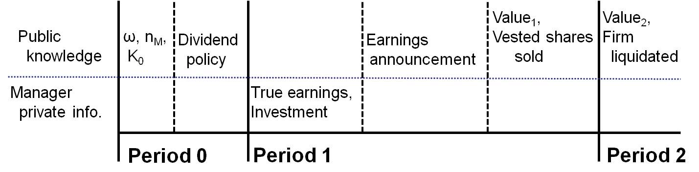
In this model, there are three periods (0, 1, 2) and two players: the manager and the shareholders. All players are risk neutral.

The manager's objective is to maximize the value of the manager's compensation package. The shareholders are represented by the board. The board and the shareholders are considered as the same player because the board and the shareholders have the same objective of maximizing the value of the firm. The board helps monitor the manager by setting the firm dividend policy.

In period zero, the board and the manager establish a contract covering the next two periods. The contract specifies an allocation of shares for the manager to be paid at the end of the first period. A portion of these shares $\omega$ will vest and will be sold after the announcement of first-period earnings.⁹ The balance of shares ( $1-\omega$ ) cannot be sold until the end of the second period, when the firm is liquidated. All shares are assumed to retain dividend rights.¹⁰ The terms of the manager's contract are public knowledge and cannot be renegotiated.

Once the contract is set, the board commits to a dividend policy. The policy designates a specific level of dividends.

The manager's contract also includes the assignment of an initial capital stock , which determines the distribution of earnings in period one. Only the manager sees true earnings. The manager has the option of using firm cash flows for productive investment or for EM, announcing earnings different from true earnings. Announcing higher earnings can potentially raise the value of the shares sold after the earnings announcement. However, the board has already established a dividend policy. Because dividends are paid out of firm cash flows, dividends limit the resources available for EM and therefore limiting the amount of price manipulation that managers can exert on firm value. Figure 1 shows the order of events for this model.

All manager compensation is equity-based. The manager can only earn more by increasing firm value.¹¹ While this form of compensation aligns the interests of the manager with shareholders, the agency problems are not entirely solved. The manager has more information about the true performance of firm operations and has control over the release of firm information. This information asymmetry could allow the manager to push the market value away from true value.¹² While this model only uses shares for compensation, the incentives are similar to managers with option portfolios. Managers will want to improve firm valuations around the time when options are exercisable.¹³

To simplify the analysis, this model does not allow for the possibility of share repurchases and does not allow for further financing from debt or equity. This model generally follows the "new view" modeling assumption that investment is done primarily out of retained earnings.¹⁴ For purposes of modeling dividend behavior, this funding assumption follows the empirical evidence that dividend payers tend to be large, highly profitable, and established firms.

3.2 True Earnings, Earnings Announcements, and Firm Valuation

Shareholders develop expectations of firm earnings based on observing industry performance and knowing initial capital. Their unconditional expectation of earnings can be denoted as $f(K_{t-1})$ , where $K_{t-1}$ is the level of capital in period and $f(\cdot)$ is the production function of the firm.

The true earnings of the firm are only known by the manager. True earnings for period one and period two, and the change in capital over time, are

$\displaystyle \pi_1$	$\displaystyle =$	$\displaystyle f(K_0)+\varepsilon_1$
$\displaystyle \pi_2$	$\displaystyle =$	$\displaystyle f(K_1)$
$\displaystyle K_1$	$\displaystyle =$	$\displaystyle (1-\delta)K_0+I_1,$	(1)

where $\delta \in [0,1)$ is the depreciation rate of capital and $\varepsilon_1$ is a production shock seen only by the manager. When period two starts, only the manager knows the amount of additional investment in capital

. Only production from period one capital determines period two earnings. At the end of the second period, the firm is liquidated.

The production function has the following properties: $f \in C^\infty$ ; $f(K)\geq 0$ ; ; ; and . The production shock has two possible values: $\varepsilon_{1,H}$ (high) and $\varepsilon_{1,L}$ (low). The probability of a low shock is $\rho$ .

After seeing true earnings in the first period, the manager must announce a level of earnings . The announcement can be different than the true earnings, but there is a cost of lying. The relationship between announced earnings and true earnings for the two periods can be written as

$\displaystyle a_1$	$\displaystyle =$	$\displaystyle \pi_1+\nu$
	$\displaystyle =$	$\displaystyle f(K_0)+\varepsilon_1+\nu$
$\displaystyle a_2$	$\displaystyle =$	$\displaystyle \pi_2-\nu$
	$\displaystyle =$	$\displaystyle f(K_1)-\nu.$

Empirically, the manager has flexibility in controlling reported earnings through accounting rules and the timing of real transactions. As suggested by the formulas above, many of these practices just change how things are counted so the timing of earnings moves from one period to another. The inflation (deflation) $\nu$ in period one is reversed in period two. However, these efforts distract the manager from identifying optimal projects, creating real costs.

These real costs lower the amount of investment which, in turn, lowers period two earnings.¹⁵ The cost has the following properties: $c \in C^\infty$ ; $c(\nu)\ge 0$ ; ; ; and . Notice that the same cost is incurred whether the manager is inflating or deflating earnings.¹⁶ The cost of changing earnings also increases at an increasing rate.

The cash flow generated by the firm is assumed to be equal to the true earnings of the firm minus the taxes payable based on announced earnings. The cashflow constraint is therefore

$\displaystyle D_1+I_1+c(\nu)$

$\displaystyle =$

$\displaystyle f(K_0)+\varepsilon_1-\tau a_1,$

(2)

where

is the dividend paid in the first period and $\tau$ is the corporate tax rate. Cash flow can be used for the dividend, for investment, or for covering the costs associated with inflating (or deflating) earnings.¹⁷

The model assumes that reported earnings are taxable. While not explicitly true for U.S. firms, this assumption avoids the potential problem that outsiders can use the information in GAAP accounting statements and tax statements to better understand the level of EM.¹⁸

Given the order of the decisions, investment is a residual. Period one capital can be calculated by combining equation 1 and equation 2:

$\displaystyle K_1$

$\displaystyle =$

$\displaystyle (1-\delta)K_0+f(K_0)+\varepsilon_1-\tau a_1-c[a_1-f(K_0)-\varepsilon_1]-D_1.$

(3)

If shareholders have perfect information about firm earnings, firm value in period zero is determined by the present value of the firm's expected payouts. To simplify the analysis, the differential tax treatment between dividends and capital gains are dropped. Let be the discount factor based on the net-of-tax rate of return an investor can get on a similar risk asset. Under perfect information, the firm value in period zero equals

$\displaystyle V_0^*$	$\displaystyle =$	$\displaystyle E_0\Big[d D_1+ d^2V_2^* \Big]$
$\displaystyle E_0[V_2^*]$	$\displaystyle =$	$\displaystyle E_0\Bigg[(1-\tau)f\Big((1-\delta)K_0+f(K_0)+\varepsilon_1-\tau a_1-c(\nu)-D_1\Big)$
		$\displaystyle +\tau\nu\Bigg].$	(4)

Equation (4) shows that even if shareholders were perfectly informed, managers will report earnings that differ from true earnings in order to minimize the present value of corporate tax payments. Let $a_1=a_{1,\theta}^*$ be the optimal announcement strategy given a $\theta$ production shock (high or low) and perfect information. The first order condition is

$\displaystyle \frac{\partial V_2^*}{\partial a_1}$

$\displaystyle =$

$\displaystyle -(1-\tau)f'(K_1)[\tau+c']+\tau=0.$

Deflating earnings by one dollar will increase the value of the firm if the after-tax marginal product of $\tau$ more dollars of capital from tax savings covers both the marginal cost of EM from moving that dollar and the delayed tax payment. If there was no corporate tax and if shareholders have perfect information, there would be no reason to misreport. See appendix A for details on the characteristics of the solution for the perfect information problem.

However, shareholders do not have perfect information about true earnings. They will use the announced earnings to update their beliefs about whether the firm received a low ( $\hat{\rho}$ ) or high $(1-\hat{\rho})$ production shock.¹⁹

$\displaystyle V_1(a_1)$

$\displaystyle =$

$\displaystyle D_1+\hat{\rho} V_{1,L}(a_1)+(1-\hat{\rho}) V_{1,H}(a_1),$

where $V_{1,\theta}(a_1)$ is the firm value in period one given that the manager reports earnings of

and has a $\theta$ -type production shock.

Shareholders can value each production shock type firm independently,

$\displaystyle V_{1,\theta'}(a_1)$	$\displaystyle =$	$\displaystyle dV_{2,\theta'}$
	$\displaystyle =$	$\displaystyle d\Big[(1-\tau)f\Big((1-\delta)K_0+f(K_0)+\varepsilon_{1,\theta'}-\tau a_1 -c[a_1-f(K_0)-\varepsilon_{1,\theta'}]-D_1\Big)$
		$\displaystyle +\tau[a_1-f(K_0)-\varepsilon_{1,\theta'}]\Big],$

where $\theta'$ is the production shock type that shareholders infer. Notice that earnings announcement depends on the production shock $\varepsilon_1$ .

3.3 Managerial Incentives

The manager uses the earnings announcement to maximize the payoff from the compensation package. The optimal earnings announcement for a manager with $\theta$ -type production shock will depend on the type $\theta'$ shareholders infer. There will be two levels of earnings announcements in a separating equilibrium, and one announcement in a pooling equilibrium. Shareholders will value a firm assuming a low production shock for any off-the-equilibrium-path announcements. The manager's maximization formula is

$\displaystyle U_{1,\theta}(a_1,\theta')$

$\displaystyle =$

$\displaystyle n_M D_1 +n_M \Big(\omega V_{1,\theta'}(a_1)+d(1-\omega)V_{2,\theta}(a_1)\Big).$

Perfect Information
Define $\hat{a}_{1,\theta}$ as a manager's announcement strategy. If shareholders know the production shock $\varepsilon_1$ perfectly, every manager will have an announcement strategy that is optimal for tax purposes $\hat{a}_{1,\theta}=a_{1,\theta}^*$ . There is no incentive to change earnings further.

Imperfect Information
If shareholders do not know the value of the production shock, managers will want to use the first-best announcement strategy.²⁰

Low Production Shock Manager
Under a separating equilibrium, managers with a low production shock know that shareholders will correctly infer from the earnings announcement that there was a low production shock. These managers will therefore optimize firm value conditional on a low shock.

$\displaystyle U_{1,L}(\hat{a}_{1,L},L)$

$\displaystyle \geq$

$\displaystyle U_{1,L}(a_{1,L},L).$

The best strategy in this case is to choose the tax optimizing announcement $\hat{a}_{1,L}=a_{1,L}^*$ .

A separating equilibrium is supported only if a manager facing a low production shock cannot do better by mimicking the announcement made by a high-shock manager. The low-shock manager will not imitate as long as

$\displaystyle U_{1,L}(a_{1,L}^*,L)$

$\displaystyle \geq$

$\displaystyle U_{1,L}(\hat{a}_{1,H},H).$

(5)

High Production Shock Manager
Because $U_{1,L}(\hat{a}_{1,H},H)$ is a declining function in $\hat{a}_{1,H}$ , this incentive constraint (equation 5) defines the minimum value that the high-shock manager can announce that will prevent mimicking. This level is denoted as $a_{1,H}^{min}$ .

Ignoring this incentive constraint, a manager with a high-type shock can choose the tax optimizing announcement and not worry about the low type mimicking. Any further exaggeration of earnings would lower investment, lowering firm value.

$\displaystyle \hat{a}_{1,H}$

$\displaystyle =$

$\displaystyle a_{1,H}^*$

However, supporting the separating equilibrium requires that

$\displaystyle U_{1,H}(a_{1,H}^{min},H)$

$\displaystyle \geq$

$\displaystyle U_{1,H}(a_{1,H}^{*},L).$

The announcement by a high-shock manager then satisfies

$\displaystyle \hat{a}_{1,H}$

$\displaystyle =$

$\displaystyle \max \Big(U_{1,H}(a_{1,H}^{min},H),\;U_{1,H}(a_{1,H}^{*},L)\Big).$

There are also pooling equilibria if the incentive constraints do not hold. A manager with a high-type shock will make the tax optimizing earnings announcement, and that announcement can be mimicked by a manager with a low-type shock. See appendix A for more details on the model solution.

3.4 Board Dividend Policy

Because the board is trying to maximize firm value, the dividend policy is designed to optimize ex ante value. The optimal dividend depends on the value of the firm in the expected equilibrium: separating or pooling. The dividend is set to help minimize exaggerated earnings announcements.

Complete Information
Optimal investment depends on the marginal product of firm capital. Under perfect information (equation 4), the first order condition for the board's maximization problem becomes²¹

$\displaystyle \frac{\partial V_0^*}{\partial D_1}: 1$

$\displaystyle =$

$\displaystyle d(1-\tau)E_0[f'(K_1)].$

Dividends will be used to pull cash out of the firm if the discounted after-tax marginal return is less than one. Let

equal the after-tax rate of return available for a similar risk asset. Then the board will use dividends to manage firm capital such that

$\displaystyle E_0[f'(K_1)] \geq 1+r.$

(6)

This equation will hold as an inequality when all earnings are left in the firm to be invested in capital. This relationship is well established in the dividend model literature.²² Given the cash flow constraint, the only role of the dividend is to determine the level of new investment.

Incomplete Information
Because the dividend policy is announced before the earnings announcement, the board will set the policy using the initial probabilities of the production shock. To optimize dividends, the board will recognize how the dividend affects the nature of the equilibrium.

The effect of dividends on firm value has two channels. There is direct effect and an indirect effect through a change in earnings announcement.

$\displaystyle V_1$	$\displaystyle =$	$\displaystyle D_1+\rho V_{1,L}(a_{1,L}(D_1),D_1)+(1-\rho)V_{1,H}(a_{1,H}(D_1),D_1)$
$\displaystyle \frac{\partial V_1}{\partial D_1}$	$\displaystyle =$	$\displaystyle 1+\rho \Big(\frac{\partial V_{1,L}}{\partial a_{1,L}}\frac{\partial a_{1,L}}{\partial D_1}+\frac{\partial V_{1,L}}{\partial D_1}\Big) + (1-\rho) \Big(\frac{\partial V_{1,H}}{\partial a_{1,H}}\frac{\partial a_{1,H}}{\partial D_1}+\frac{\partial V_{1,H}}{\partial D_1}\Big) =0$	(7)

If there is a pooling equilibrium, the board will simply use equation 6 to set dividends, where there is a strict inequality when . Because the board maximizes ex ante firm value, the ex post investment will be too high if the production shock is high, and the ex post investment will be too low if the production shock is low.

If a separating equilibrium exists such that both manager types announce the tax-optimizing level of earnings, the board will again use equation 6 to set the dividend, where there is a strict inequality when . Notice that the first term in each set of parenthesis (equation 7) equals zero due to the envelope rule.

If a separating equilibrium is supported by high types announcing exaggerated earnings $a_{1,H}^{min}$ , earnings higher than the optimal for tax purposes, the value of the firm is not optimized $\Big(\frac{\partial V_{1,H}}{\partial a_{1,H}^{min}}\frac{\partial a_{1,H}^{min}}{\partial D_1} >0\Big)$ . In these cases, dividends have an added benefit on firm value. Dividends lower announcements, lowering EM costs.

$\displaystyle U_{1,L}(a_{1,L}^*,L)$	$\displaystyle \equiv$	$\displaystyle U_{1,L}(a_{1,H}^{min},H)$
$\displaystyle \frac{\partial a_{1,H}^{min}}{\partial D_1}$	$\displaystyle =$	$\displaystyle \frac{\frac{\partial U_{1,L}(a_{1,L}^*,L)}{\partial D_1}-\frac{\partial U_{1,L}(a_{1,H}^{min},H)}{\partial D_1}}{\frac{U_{1,L}(a_{1,H}^{min},H)}{\partial a_{1,H}^{min}}}<0$

Proof of this relationship is in appendix A. Because low types have a higher marginal product of capital, mimicking low types face higher costs to exaggerating earnings and are harmed more by dividends. A higher dividend causes the incentive constraint to hold at a lower value for $a_{1,H}^{min}$ . Less value is lost because the self-selection constraint becomes less binding.

3.5 Sudden Decrease in the Size of Information Asymmetry

Now assume there is a large decrease in the amount of information asymmetry between the manager and shareholders. Auditors could have become instantaneously more vigilant or law changes could make EM more costly. SOX and the overall change in the corporate environment in the early 2000s have aspects of these two pressures. These forces would cause the EM cost function to increase to $\tilde{c}$ such that: $\tilde{c}(x)\geq c(x)$ , $\forall\; x$ ; $\tilde{c} \in C^\infty$ ; $\tilde{c}(0)=0$ ; $\tilde{c}(-x)=\tilde{c}(x)$ ; and $\tilde{c}gt;0$ .

Under this new information regime, EM is more expensive. The new regulations force more reporting and make it harder to change the timing of earnings. As a result, managers report earnings closer to the truth.

The information shock affects all firms, but managers at dividend paying firms were already being constrained by board dividend policy. As shown in the last subsection (3.4), a manager at a nondividend paying firm has more freedom to manage earnings. As a result, the information regime change is more likely to constrain the earnings announcement of managers at nondividend paying firms than dividend paying firms.

3.6 Predictions

Based on the model described above, the following relationships are predicted. These relationships will be tested in the next section (4).

P1: If dividends help limit the use of EM, managers at dividend paying firms will show less EM behavior than those at nondividend paying firms.

P2: If SOX or the overall change in the accounting environment increased the amount of financial disclosure in company financial statements, the information asymmetry between shareholders and the manager should have decreased. Given that EM is a proxy for the size of the information gap, the amount of EM should have decreased following SOX.

P3: Given that managers at dividend paying firms are more constrained in their use of EM, the drop in EM will be less for dividend paying firms than nondividend paying firms following the passage of SOX.

4 Testing for Earnings Management

4.1 Data

The data for all of the analyses in this paper come from the COMPUSTAT North America Fundamentals Annual database and the Center for Research in Security Prices (CRSP) database available through Wharton Research Data Services. The COMPUSTAT database contains market and financial data on public U.S. firms. The CRSP database has daily stock price and dividend data for U.S. firms. Only data on the public firms trading on the NYSE, AMEX, or NASDAQ are used for this paper. In statistical terms, the general data set is an unbalanced panel because firms enter and leave the data set as firms get listed on these exchanges, delist, go bankrupt, or are acquired.²³

Following past research, the samples exclude financial companies and utilities because these industries have regulations on capital. These regulations influence earnings motives and the ability to return earnings to shareholders through dividends (Chetty and Saez [2005]).²⁴

4.2 Estimates of Discretionary Accruals

An extensive amount of accounting research has focused on ways to model or detect EM. Because modeling techniques can only proxy for actual EM, using these methods is a test of both the detection model and the use of EM. Despite these limitations, expected accrual models are widely adopted by researchers.²⁵ Because there is no consensus on the best model to use, several methods of proxying for EM are used in this paper.

The seminal work by Jones (1991) showed a method to estimate the amount of manipulation by comparing a firm's reported accruals to expected accruals. Several papers since then have improved upon this method. Four primary models are reported in this paper: three models are variations of the Jones model and one model is a performance matching model suggested by Kothari, et al. (2005).

The overall goal of these expected accrual models is to obtain a measure of discretionary accruals (DA), accruals that are more easily controlled by managers. Any change in total accruals (TA) comes from changes in DA and normal accruals (NA), accruals that come about through standard firm operations and that are less open to control.

$\displaystyle \Delta TA_t = (DA_t-DA_{t-1})+(NA_t-NA_{t-1})$

Jones modeled expected accruals based on observable firm characteristics. The first model in this paper will follow her basic technique and include a constant in the regression to help reduce heteroskedasticity not handled by deflating the variables with lagged assets and to help control for problems related to an omitted scale variable (Brown, Lo, and Lys [1999] and Kothari, Leone, and Wasley [2005]). The primary regression is²⁶

$\displaystyle \frac{TA_{i,t}}{A_{i,t-1}(6)} = \alpha_{0}+\alpha_{1}\Big(\frac{1}{A_{i,t-1}(6)}\Big)+\beta_{1}\Big(\frac{\Delta REV_{i,t}(12)}{A_{i,t-1}(6)}\Big) +\beta_{2}\Big(\frac{PPE_{i,t}(7)}{A_{i,t-1}(6)}\Big)+\varepsilon_{i,t}.$

(8)

The level of total accruals required by firm depends on firm size measured by lagged total assets (), on the change in firm revenues ( $\Delta REV$ ), and on the firm's fixed capital, proxied by property, plant, and equipment (). Everything is scaled by lagged total assets. Regressions are run at the industry level (two-digit SIC) for each year. Each year-industry regression must have at least ten firm-year observations to be included in this analysis.²⁷

Total accruals for all the models reported in this paper are defined following Dechow, et al. (1995) and Kothari, et al. (2005) (KLW).²⁸

$\displaystyle TA$	$\displaystyle =$	$\displaystyle [\Delta$ Current Assets $\displaystyle (4)-\Delta$ Cash $\displaystyle (1)]$
		$\displaystyle -[\Delta$ Current Liabilities $\displaystyle (5)-\Delta$ Current Maturities of LT Debt $\displaystyle (34)]$
		$\displaystyle -$ Depreciation and Amortization Expense $\displaystyle (14)$

DA are estimated by taking the difference between reported accruals and expected accruals.

$\displaystyle \hat{DA}_{i,t}$	$\displaystyle =$	$\displaystyle \hat{\varepsilon}_{i,t}$
	$\displaystyle =$	$\displaystyle \frac{TA_{i,t}}{A_{i,t-1}}-\hat{\alpha}_{0}-\hat{\alpha}_{1}\Big(\frac{1}{A_{i,t-1}}\Big) -\hat{\beta}_{1}\Big(\frac{\Delta REV_{i,t}}{A_{i,t-1}}\Big) -\hat{\beta}_{2}\Big(\frac{PPE_{i,t}}{A_{i,t-1}}\Big)$

Positive DA are evidence of inflating earnings. Negative DA are evidence of deflating earnings.

The second Jones model ("Modified Jones") works the same except the regression formula (equation 8) has a change in the revenue term to $\beta_{1}\Big(\frac{\Delta REV_{i,t}(12)-\Delta REC_{i,t}(2)}{A_{i,t-1}(6)}\Big)$ , where is accounts receivable (Dechow, Sloan, and Sweeney [1995]). By taking out the change in receivables, this form of the model assumes that changes in credit sales are discretionary. This type of model is better suited to detect EM achieved through methods such as volume sales near the end of a reporting period.²⁹

The third Jones model ("Jones with ROA") is another variation of the total accruals regression formula. It includes return on assets (ROA) on the right-hand side.³⁰ KLW argue that including ROA helps improve specifications where there are periods of abnormal returns. However, KLW also point out that there are many reasons to expect that ROA does not affect accruals linearly. According to their tests, a model matching on performance (current year ROA) performs the best.

This performance-matching model ("Performance KLW") is the fourth DA measure reported in this paper. The Performance KLW DA for firm in year is defined as the Jones DA for firm in year minus the Jones DA for the firm with the closest ROA in the same 2-digit SIC code and the same year.³¹ Effectively, this proxy of EM defines DA relative to a firm's closest industry peer by ROA.

The dividend model in this paper predicted that dividend paying firms will have lower levels of EM than nondividend paying firms and that EM will fall after SOX. Because DA is positive or negative depending on whether the manager is inflating or deflating earnings, evidence of earnings management will be proxied by the absolute value of DA.

Given a hypothesis about managing earnings for a specific event, some researchers use an alternative strategy of modeling accruals by using a pre-event estimation period. SOX is a testable event, but it also changed the disclosure rules. Using a pre-event estimation technique assumes a non-time varying relationship between normal accruals and firm characteristics. It is likely that SOX changed these relationships, making the results from a pre-event estimation strategy biased. Comparing firm accrual behavior within the year will help identify those firms that had abnormal changes in accruals versus peers in the same period.

4.3 Initial Results of Discretionary Accruals Testing

Figure 2 shows how the median absolute value of DA has changed between 1980 and 2008 using the four primary models described in section 4.2. Before taking the absolute value, each DA measure has been winsorized at the top and bottom 1 percent of the distribution. Across all models, nondividend payers consistently have a higher level of absolute DA. Nondividend payers show more evidence of EM than dividend payers. This difference remains the case as the composition of firms in the sample changes, as shown in the bottom panel.³²

Figure 3 focuses on the time period around the passage of SOX. The vertical line separates the pre-SOX and post-SOX periods. Recall that SOX was passed in July 2002. Given that all the firms in this sample have a December fiscal year end, December 2002 was the first financial report under the new law. Not all of the aspects of SOX were phased in by this point, but the officers did have to certify their financial reports.

For each model, dividend payers have roughly the same median absolute value of DA throughout the period, but there is a drop in the same measure for nondividend payers between the pre- and post-SOX periods. The graphs suggest that the peak of EM behavior was around 2000, well before SOX. This early change in behavior may have been in response to a changing environment. The stock market had peaked, and the Arthur Andersen-Enron case was unfolding. According to all of the models, median absolute DA for nondividend payers fell both in 2001 and in 2002. These results are consistent with other research on DA and SOX (Cohen, Dey, and Lys [2008] and Lobo and Zhou [2006]).

Overall, this initial DA evidence supports the three predictions developed from the theoretical model. Dividend payers use less EM than nondividend payers (P1). Firms use less EM after SOX (P2). SOX changed the behavior of nondividend payers more than dividend payers (P3).

4.4 Regressions with Discretionary Accruals

To further examine a possible behavior change following SOX and the relationship between dividends and EM, this section reports regressions of absolute DA on payout policy and firm characteristics.

Table 1 shows the summary statistics of the data used in the DA models and for the regressions in this section. The time window is narrowed to the four annual reports before and after SOX (data from December 1998 to December 2005). Table 2 shows the DA measures broken down for all firms, for nondividend payers, and for dividend payers. Notice that the means of the discretionary accruals for all firms (first four rows in table 2) are near zero. These means should be zero by design because the discretionary accrual is the regression residual. However, these data have been winsored at the bottom and top 1 percent.

As expected based on the prior graphs, the mean and median of absolute DA for nondividend payers are higher than those of dividend payers. The mean/standard deviation ratio is shown in the last column of table 2. According to all models, dividend payers have lower relative variation in the absolute level of DA.

The baseline regression is constructed to test the three predictions.

$\displaystyle abs(DA_{i,t})$	$\displaystyle =$	$\displaystyle \alpha+\beta_1$ Dividend payer $\displaystyle _{i,t}+\beta_2$ SOX $\displaystyle _t*$ Dividend payer $\displaystyle _{i,t}$
		$\displaystyle +$ year dummies	(9)

Dividend payer $_{i,t}$ and SOX

are dummy variables. Dividend payer $_{i,t}$ equals one if the firm

paid a dividend in year

and equals zero otherwise. SOX

equals one for all periods after the passage of SOX, where December 2002 is the first such period. The baseline model specification (equation 9) also includes year dummies.

According to the theoretical model, dividend payers use less EM. Because absolute DA is a proxy for EM, dividend payers should have lower absolute DA (P1). The expected sign of the coefficient on Dividend payer $_{i,t}$ is negative. The theoretical model shows that managers should use less EM after SOX due to its higher cost. Absolute DA should be lower following SOX (P2). Therefore, the coefficients for the year dummies should be lower for years following SOX than for those pre-SOX. Given that dividend payers are already constrained by the dividend, SOX should not affect DA behavior as much as for nondividend payers (P3). The interacted term should counteract the year dummies, making the expected sign on the interacted term positive.

Table 3 reports the results of the baseline regression. The successive columns separately test the four primary DA measures. The signs of all the primary coefficients are as expected and statistically significant, and the year dummy coefficients follow the expected pattern. The difference between the 2001 and 2002 dummy variables is 1 percent across all models, and tests of whether the coefficients are equal are rejected. Also notice that absolute DA fell by roughly 2 percent between 2000 and 2001. However, dividend payers did not experience the same drop. As expected, the coefficient on the interacted term offsets the SOX decrease. The coefficient is about 3 percent for all of the models, more than offsetting the SOX drop. This excess may be due to the previously mentioned 2-percent drop between 2000 and 2001. Recall that the DA measures are scaled by assets. The units are DA as a share of assets. These regression results suggest that nondividend payers shrank the composition of their assets consisting of DA by 1 percent after SOX.

The theoretical model also showed that the amount of earnings management depends on the marginal product of firm capital. The marginal product of capital can be proxied by firm characteristics such as size, life cycle, and profitability. The next set of specifications use the four firm characteristic variables Fama & French (2001) included in their study on dividend payers.³³

$\displaystyle abs(DA_{i,t})$	$\displaystyle =$	$\displaystyle \alpha+\beta_1$ Dividend payer $\displaystyle _{i,t}+\beta_2$ SOX $\displaystyle _t*$ Dividend payer $\displaystyle _{i,t}$
		$\displaystyle +\beta_3$ NYSE market capitalization $\displaystyle _{i,t}+\beta_4\frac{\mbox{Value}_{i,t}}{\mbox{Assets}_{i,t-1}}$
		$\displaystyle +\beta_5$ Asset growth $\displaystyle _{i,t} + \beta_6\frac{\mbox{Earnings}_{i,t}}{\mbox{Assets}_{i,t-1}}$
		$\displaystyle +$ year dummies	(10)

NYSE market capitalization is a proxy of size. It is equal to the percentage of NYSE firms that have the same or a lower market capitalization (takes a value between zero and one). The Value/Lagged assets measure, also known as the market-to-book ratio, is similar to Tobin's q. Young firms that are expected to grow and become more profitable in the future are highly valued by the market. These firms tend to trade at a higher ratio than older firms; it is a proxy for life cycle. Asset growth is another proxy for life cycle under the assumption that younger firms grow faster than older firms. Earnings/Lagged assets is a profitability measure and provides another measure for the opportunity cost of capital.³⁴

The expected sign on NYSE market capitalization is positive. Larger firms tend to be more mature and have a lower opportunity cost of earnings management. It may also be easier for large firms to move earnings. The signs on the life-cycle variables of market-to-book and asset growth are expected to be negative. Younger firms should have a high marginal product of capital. The expected sign of the profitability measure is also negative. Profitable firms have a higher opportunity cost, making EM more expensive for the manager.

Table 4 reports the regression results of this new specification with firm characteristics. The sign and significance of the coefficient on Dividend payer and that on the interacted term remain. However, the coefficient on Dividend payer changes from roughly -3 percent in the baseline to -2 percent. The expected patterns on the year dummy coefficients remain. These coefficients suggest that DA fell 1 percent between 2001 and 2002 and fell 1 to 2 percent between 2000 and 2001.

Three of the four coefficients on the firm characteristic variables are statistically significant, but two of them have signs that are opposite to expectations: NYP and Value/Lagged assets. Larger firms (NYP) should have relatively low marginal product of capital and, therefore, cheaper EM. These firms should have more evidence of EM than smaller firms. Firms with high Value/Lagged assets, and therefore, more expensive EM, should tend to be firms with expectations of strong growth and less evidence of EM. These results suggest the opposite. Possible reasons for these results are that larger firms may be more closely scrutinized, making EM more difficult. Firms with high Value/Lagged assets are likely to be younger firms and likely to have more intangible assets. Both of these characteristics are related to having more hidden information, making earnings announcements affect stock prices more and, therefore, creating stronger incentives for the manager.

While the firm characteristics help control for firms that are likely to pay dividends, it is likely that other firm characteristics affect both dividend payment and DA. To help control for unobservables, the next set of regressions use firm fixed effects and are shown in table 5.

The signs on Dividend payer and the interacted term continue to match expectations. Only the interacted term coefficient is statistically significant, and it remains around 1 percent. By using fixed effects, these coefficients are identified by firms that switch dividend policy. Yet, the point estimate on Dividend payer suggests that firms switching to pay a dividend have lower DA. While each year there are firms that switch to become dividend payers, many firms became dividend payers following the dividend tax reform in 2003.³⁵

The expected patterns on the year dummy coefficients also remain. These coefficients suggest that DA fell 1 percent both between 2001 and 2002 and between 2000 and 2001. The signs of the coefficients on the firm characteristics generally follow expectations when they are statistically significant with the exception of Value/Lagged assets.

As suggested by the graphs in figure 3 and the regression tests, absolute DA began falling in 2001. This early change in behavior may have been a result of a change in the corporate environment. Managers were using less aggressive accounting because of such things as the Arthur Andersen-Enron scandal. As a robustness check, I change the SOX cutoff from 2002 to 2001 and rerun the tests. For space reasons, the regression results are not reported in this paper, but the general results still hold. The signs for the primary variables of Dividend payer and the interacted term match expectations. Both coefficients are statistically significant in the baseline regression and a regression with firm characteristic variables. The Dividend payer coefficient is not statistically different from zero when fixed effects are used. The expected patterns on the year dummy coefficients also remain; the dummies for 1999 and 2000 are statistically different and higher than 2001 and later.

There is still a concern about the unobserved characteristics of firms. The dividend literature suggests that dividend payers are different types of firms than nondividend payers. Perhaps the same characteristics related to dividend payment are related to DA but are not tied to the mechanisms in my model, or the same characteristics related to dividend payment are related to predictable accruals. As a robustness check, I try to identify nondividend paying firms that most look like dividend payers and compare the DA of those firms to those of dividend paying firms. To identify nondividend paying firms that look like dividend payers, I use the logit model used by Fama & French (2001).

$\displaystyle logit($ Dividend payer $\displaystyle =1)$	$\displaystyle =$	$\displaystyle \alpha+\beta_1$ NYSE market capitalization $\displaystyle _{i,t}$
		$\displaystyle +\beta_2\frac{\mbox{Value}_{i,t}}{\mbox{Assets}_{i,t-1}} +\beta_3\mbox{Asset growth}_{i,t}$
		$\displaystyle +\beta_4\frac{\mbox{Earnings}_{i,t}}{\mbox{Assets}_{i,t-1}}+\mbox{industry dummies}$	(11)

I run equation 11 separately for each year. The estimated coefficients are then used to generate probabilities of being a dividend payer. Those firm observations that have an estimated probability greater than 0.5 are then used for DA regression testing. Table 6 summarizes the results of these logit regressions. Notice that around 200 nondividend paying firms are included each year.

The DA regression results are shown in table 7. For three of the four models, the primary conclusions still hold: dividend paying firms use less EM, evidence of EM fell after SOX, and nondividend paying firms changed their behavior more than dividend paying firms.³⁶

5 Concluding Remarks

The challenge of optimizing manager behavior for shareholder value has two primary parts. First, the manager has different incentives than shareholders--agency problems. Second, the manager knows much more about the financial viability of the firm than shareholders--information asymmetry. Both of these elements need to be incorporated into dividend models to understand the dynamics of payout selection. Conflicting incentives explain manager behavior given compensation packages and ownership structure, but incentives alone do not explain payout dynamics following tougher reporting standards or explain how shareholders might learn more about the extent of agency problems.

The model presented in this paper was designed to explore the relationships among dividend policy decisions, information asymmetry, and managerial incentives. The model shows and the tests confirm that EM behavior is different depending on payout policy. According to the DA tests, dividend payers did not appear to change their reporting behavior as much as nondividend payers after the passage of SOX. Furthermore, dividend payers consistently have lower absolute DA. This lower absolute DA is evidence that dividend payers inflate and deflate earnings less than nondividend payers.

The model presented here posits that dividends help limit the discretion of management, leading to more-truthful earnings reports. The dividend commitment is possible through a board that is perfectly aligned with shareholders. Further work is needed to evaluate how board composition relates to monitoring levels and payout policy.³⁷ Overall, the findings presented here suggest that dividend policies are effective at limiting information asymmetries.

Bibliography

D. Aboody & R. Kasznik (2000).

`CEO Stock Option Awards and the Timing of Corporate Voluntary Disclosures'.
Journal of Accounting & Economics 29:73-100.

A. J. Auerbach (1979).

`Wealth Maximization and the Cost of Capital'.
The Quarterly Journal of Economics 93(3):433-446.

A. J. Auerbach & K. A. Hassett (2005).

`The 2003 Dividend Tax Cuts and the Value of the Firm: An Event Study. Working Paper, NBER, No. 11449'.

J. C. Bettis, et al. (2000).

`Corporate Policies Restricting Trading by Insiders'.
Journal of Financial Economics 57(2):191-220.

S. Bhattacharya (1979).

`Imperfect Information, Dividend Policy, and "The Bird in the Hand" Fallacy'.
The Bell Journal of Economics 10(1):259-270.

D. F. Bradford (1981).

`The Incidence and Allocation Effects of a Tax on Corporate Distributions'.
Journal of Public Economics 15(1):1-22.

A. Brav, et al. (2005).

`Payout Policy in the 21st Century'.
Journal of Financial Economics 77:483-527.

S. Brown, et al. (1999).

`Use of

in Accounting Research: Measuring Changes in Value Relevance over the Last Four Decades'.
Journal of Accounting & Economics 28(2):83-115.

P. K. Chaney & C. M. Lewis (1995).

`Earnings Management and Firm Valuation under Asymmetric Information'.
Journal of Corporate Finance 1(3-4):319-345.

R. Chetty & E. Saez (2005).

`Dividend Taxes and Corporate Behavior: Evidence From the 2003 Dividend Tax Cut'.
The Quarterly Journal of Economics 120(3):791-833.

R. Chetty & E. Saez (2007).

`An Agency Theory of Dividend Taxation. Working Paper, NBER, No. 13538'.

I.-K. Cho & D. M. Kreps (1987).

`Signaling Games and Stable Equilibria'.
The Quarterly Journal of Economics 102(2):179-222.

J. C. Coates IV (2007).

`The Goals and Promise of the Sarbanes-Oxley Act'.
Journal of Economic Perspectives 21(1):91-116.

D. A. Cohen, et al. (2008).

`Real and Accrual-Based Earnings Management in the Pre- and Post-Sarbanes-Oxley Periods'.
The Accounting Review 83(3):757-787.

N. D. Daniel, et al. (2008).

`Do Firms Manage Earnings to Meet Dividend Thresholds?'.
Journal of Accounting & Economics 45:2-26.

H. DeAngelo, et al. (1996).

`Reversal of Fortune: Dividend Signaling and the Disappearance of Sustained Earnings Growth'.
Journal of Financial Economics 40:341-371.

H. DeAngelo, et al. (2006).

`Dividend Policy and the Earned/Contributed Capital Mix: A Test of the Life-Cycle Theory'.
Journal of Financial Economics 81:227-254.

P. M. Dechow & I. D. Dichev (2002).

`The Quality of Accruals and Earnings: The Role of Accrual Estimation Errors'.
The Accounting Review 77:35-59.

P. M. Dechow & C. M. Schrand (2004).

Earnings Quality.
The Research Foundation of CFA Institute, Charlottesville, VA.

P. M. Dechow, et al. (1995).

`Detecting Earnings Management'.
The Accounting Review 70(2):193-225.

F. H. Easterbrook (1984).

`Two Agency-Cost Explanations of Dividends'.
American Economic Review 74(4):650-659.

M. Erickson, et al. (2004).

`How Much Will Firms Pay for Earnings That Do Not Exist? Evidence of Taxes Paid on Allegedly Fraudulent Earnings'.
The Accounting Review 79(2):387-408.

E. F. Fama & K. R. French (2001).

`Disappearing Dividends: Changing Firm Characteristics or Lower Propensity to Pay?'.
Journal of Financial Economics 60:3-43.

R. Gordon & M. Dietz (2006).

`Dividends and Taxes. Working Paper, NBER, No. 12292'.

P. M. Healy (1985).

`The Effect of Bonus Schemes on Accounting Decisions'.
Journal of Accounting & Economics 7:85-107.

P. M. Healy & K. G. Palepu (2001).

`Information Asymmetry, Corporate Disclosure, and the Capital Markets: A Review of the Empirical Disclosure Literature'.
Journal of Accounting & Economics 31:405-440.

M. C. Jensen (1986).

`Agency Costs of Free Cash Flow, Corporate Finance, and Takeovers'.
American Economic Review 76(2):323-329.

K. John & A. Knyazeva (2006).

`Payout Policy, Agency Conflicts, and Corporate Governance. Working Paper, New York University, New York, NY'.

J. J. Jones (1991).

`Earnings Management During Import Relief Investigations'.
Journal of Accounting Research 29(2):193-228.

E. Kasanen, et al. (1996).

`Dividend-Based Earnings Management: Empirical Evidence from Finland'.
Journal of Accounting & Economics 22(1-3):283-312.

B. Kay & C. M. Vojtech (2011).

`How Do Firms Switch Among Tools Used to Monitor Agency Problems? Working Paper, University of California-San Diego, La Jolla, CA'.

S. P. Kothari, et al. (2005).

`Performance Matched Discretionary Accrual Measures'.
Journal of Accounting & Economics 39:163-197.

G. J. Lobo & J. Zhou (2006).

`Did Conservatism in Financial Reporting Increase After the Sarbanes-Oxley Act? Initial Evidence'.
Accounting Horizons 20(1):57-73.

D. J. Lucas & R. L. McDonald (1990).

`Equity Issues and Stock Price Dynamics'.
Journal of Finance 45(4):1019-1043.

M. H. Miller & K. Rock (1985).

`Dividend Policy Under Asymmetric Information'.
Journal of Finance 40(4):1031-1051.

K. J. Murphy (1999).

Executive Compensation, in: Ashenfelter,O., Card,D. (Eds.), vol. 3 of Handbook of Labor Economics, pp. 2485-2563.
Elsevier, Amsterdam.

S. E. Perry & T. H. Williams (1994).

`Earnings Management Preceding Management Buyout Offers'.
Journal of Accounting & Economics 18:157-179.

S. Savov (2006).

`Earnings Management, Investment, and Dividend Payments. Working Paper, University of Mannheim, Mannheim, Germany'.

K. Schipper (1989).

`Commentary on Earnings Management'.
Accounting Horizons 3(4-5):91-102.

D. J. Skinner & E. Soltes (2011).

`What Do Dividends Tell Us About Earnings Quality?'.
Review of Accounting Studies 16(1):1-28.

S. H. Teoh, et al. (1998a).

`Earnings Management and the Underperformance of Seasoned Equity Offerings'.
Journal of Financial Economics 50:63-99.

S. H. Teoh, et al. (1998b).

`Are Accruals During Initial Public Offerings Opportunistic?'.
Review of Accounting Studies 3:175-208.

U.S. Congress (2002).

`Sarbanes-Oxley Act of 2002'.

R. L. Watts (2003a).

`Conservatism in Accounting Part I: Explanations and Implications'.
Accounting Horizons 17(3):207-221.

R. L. Watts (2003b).

`Conservatism in Accounting Part II: Evidence and Research Opportunities'.
Accounting Horizons 17(4):287-301.

**Figure 1:** Order of Events for Model

**Figure 2:** Discretionary Accruals, by Model and by Payer Type [DA/Lagged assets]

**Figure 3:** Discretionary Accruals, by Model and by Payer Type [DA/Lagged assets]

Table 1: Summary Statistics for Primary Variables
Variable	Mean	Median	Std. dev.
Total accrual/ Lagged assets	-0.055	-0.047	0.643
1/ Lagged assets	0.017	0.004	0.050
Sales Chg/ Lagged assets	0.156	0.075	1.679
(Sales Chg - Rec Chg)/ Lagged assets	0.130	0.063	1.553
PPE/ Lagged assets	0.588	0.446	0.567
ROA	-0.012	0.054	0.245
NYSE market capitalization	0.350	0.282	0.301
Value/ Lagged assets	2.991	1.694	6.517
Asset growth	0.234	0.063	2.310
Earnings/ Lagged assets	-0.011	0.057	0.330

Statistics based on data between 1998 and 2005 from 12,334 firm-year observations. Total accrual $= [\Delta$ Current Assets $(4)-\Delta$ Cash $(1)]-[\Delta$ Current Liabilities $(5)-\Delta$ Current Maturities of LT Debt

Depreciation and Amortization Expense

. COMPUSTAT data items are in parenthesis. See appendix B for more details on variable definitions and on the specific COMPUSTAT variables used.

Table 2: Summary Statistics of DA Model Results, by Payer Type (Discretionary accruals (scaled by lagged assets))
Variable	Mean	Median	Std. dev.	Mean/Std. dev.
All-12,334 firm-year observations: Jones	0.0015	0.0036	0.1409	0.011
All-12,334 firm-year observations: Modified Jones	0.0016	0.0030	0.1422	0.011
All-12,334 firm-year observations: Jones with ROA	0.0009	0.0009	0.1335	0.007
All-12,334 firm-year observations: Performance KLW	0.0015	0.0000	0.1974	0.007
All-12,334 firm-year observations: abs(Jones)	0.0634	0.0379	0.1258	0.504
All-12,334 firm-year observations: abs(Modified Jones)	0.0643	0.0386	0.1269	0.507
All-12,334 firm-year observations: abs(Jones with ROA)	0.0621	0.0377	0.1182	0.525
All-12,334 firm-year observations: abs(Modified Jones with ROA)	0.0628	0.0381	0.1192	0.527
All-12,334 firm-year observations: abs(Performance KLW)	0.0933	0.0577	0.1739	0.537
All-12,334 firm-year observations: abs(Perform KLW Modified)	0.0946	0.0584	0.1753	0.540
Nondividend payers-8,991 firm-year observations: abs(Jones)	0.072	0.043	0.144	0.500
Nondividend payers-8,991 firm-year observations: abs(Modified Jones)	0.073	0.044	0.145	0.504
Nondividend payers-8,991 firm-year observations: abs(Jones with ROA)	0.070	0.043	0.135	0.522
Nondividend payers-8,991 firm-year observations: abs(Performance KLW)	0.104	0.065	0.198	0.525
Dividend payers-3,343 firm-year observations: abs(Jones)	0.0402	0.0280	0.0430	0.933
Dividend payers-3,343 firm-year observations: abs(Modified Jones)	0.0408	0.0283	0.0443	0.921
Dividend payers-3,343 firm-year observations: abs(Jones with ROA)	0.0396	0.0280	0.0419	0.947
Dividend payers-3,343 firm-year observations: abs(Performance KLW)	0.0649	0.0433	0.0721	0.900

Table 2 (con't)
Summary Statistics of DA Model Results, by Payer Type

Dividend paying status is based on whether a dividend is paid in year

. Discretionary accruals from the Jones model are estimated for each industry and year using the residual from the following regression: $\frac{TA_{i,t}}{A_{i,t-1}(6)} = \alpha_{0}+\alpha_{1}\Big(\frac{1}{A_{i,t-1}(6)}\Big)+\beta_{1}\Big(\frac{\Delta REV_{i,t}(12)}{A_{i,t-1}(6)}\Big) +\beta_{2}\Big(\frac{PPE_{i,t}(7)}{A_{i,t-1}(6)}\Big)+\varepsilon_{i,t}$ ; where $TA_{i,t}= [\Delta$ Current Assets $(4)-\Delta$ Cash $(1)]-[\Delta$ Current Liabilities $(5)-\Delta$ Current Maturities of LT Debt

Depreciation and Amortization Expense

.
COMPUSTAT data items are in parenthesis. $\Delta REV_{i,t}$ is change in sales, and $PPE_{i,t}$ is property, plant and equipment. DA from the Modified Jones model changes the revenue term to $\beta_{2}\Big(\frac{\Delta REV_{i,t}(12)-\Delta REC_{i,t}(2)}{A_{i,t-1}(6)}\Big)$ to the first equation, where

is accounts receivable. DA from the Jones Model with ROA are similar to the Jones model except for the inclusion of current year's ROA as an additional explanatory variable. To obtain the Performance KLW model DA for firm

the Jones model DA of the firm with the closest ROA that is in the same industry as firm

. DA variables are winsorized at the 1st and 99th percentiles before taking the absolute value. Statistics based on DA between 1998 and 2005.

The table reports the coefficients from the following regression: $abs(DA_{i,t}) = \alpha+\beta_1$ Dividend payer $_{i,t}+\beta_2$ SOX

Dividend payer $_{i,t} +$ year dummies; where $abs(DA_{i,t})$ is the absolute value of discretionary accruals estimated by various models separately shown in each column.

Table 3: Baseline Regression
VARIABLES	Exp. sign	(1) abs(Jones)	(2) abs(Jones Mod)	(3) abs(Jones w/ ROA)	(4) abs(KLW Perform)
Dividend payer	-	-0.0307***	-0.0313***	-0.0296***	-0.0309***
Dividend payer (Standard Error)		(0.00177)	(0.00181)	(0.00169)	(0.00224)
SOX*Div. payer	+	0.0114***	0.0114***	0.0106***	0.00877***
SOX*Div. payer (Standard Error)		(0.00214)	(0.00219)	(0.00204)	(0.00280)
Yr_99		0.00268	0.00158	0.00182	-0.00347
Yr_99 (Standard Error)		(0.00200)	(0.00208)	(0.00199)	(0.00279)
Yr_00		0.00866***	0.00680***	0.00676***	0.00183
Yr_00 (Standard Error)		(0.00234)	(0.00240)	(0.00223)	(0.00308)
Yr_01		-0.00934***	-0.00993***	-0.00875***	-0.0140***
Yr_01 (Standard Error)		(0.00198)	(0.00204)	(0.00186)	(0.00275)
Yr_02		-0.0175***	-0.0193***	-0.0169***	-0.0230***
Yr_02 (Standard Error)		(0.00213)	(0.00219)	(0.00206)	(0.00285)
Yr_03		-0.0169***	-0.0180***	-0.0155***	-0.0217***
Yr_03 (Standard Error)		(0.00225)	(0.00233)	(0.00217)	(0.00300)
Yr_04		-0.0200***	-0.0208***	-0.0159***	-0.0259***
Yr_04 (Standard Error)		(0.00217)	(0.00223)	(0.00215)	(0.00290)
Yr_05		-0.0183***	-0.0200***	-0.0158***	-0.0254***
Yr_05 (Standard Error)		(0.00220)	(0.00226)	(0.00216)	(0.00295)
Constant		0.0735***	0.0760***	0.0716***	0.103***
Constant (Standard Error)		(0.00174)	(0.00180)	(0.00168)	(0.00229)
Observations		12,334	12,334	12,334	12,334
Number of id		2,595	2,595	2,595	2,595
R-squared		0.058	0.057	0.053	0.039
Adj. R-squared		0.0574	0.0565	0.0523	0.0380

Robust standard errors in parentheses are clustered at the firm level. *** p

0.01, ** p

0.05, * p

0.10

Table 3 (con't)
Baseline Regression

Dividend paying status is based on whether a dividend is paid in year

Depreciation and Amortization Expense

the Jones model DA of the firm with the closest ROA that is in the same industry as firm

. DA variables are winsorized at the 1st and 99th percentiles before taking the absolute value. Statistics based on DA between 1998 and 2005.

The table reports the coefficients from the following regression: $abs(DA_{i,t}) = \alpha+\beta_1$ Dividend payer $_{i,t}+\beta_2$ SOX

Dividend payer $_{i,t}+\beta_3$ NYSE market capitalization $_{i,t}+\beta_4\frac{\mbox{Value}_{i,t}}{\mbox{Assets}_{i,t-1}} +\beta_5\mbox{ Asset growth}_{i,t} + \beta_6\frac{\mbox{Earnings}_{i,t}}{\mbox{Assets}_{i,t-1}} +\mbox{ year dummies}$ ; where $abs(DA_{i,t})$ is the absolute value of discretionary accruals estimated by various models separately shown in each column.

Table 4: Regression with Firm Characteristics
VARIABLES	Exp. sign	(1) abs(Jones)	(2) abs(Jones Mod)	(3) abs Jones w/ ROA)	(4) abs(KLW Perform)
Dividend payer	-	-0.0186***	-0.0189***	-0.0177***	-0.0174***
Dividend payer (Standard Error)		(0.00184)	(0.00190)	(0.00176)	(0.00234)
SOX*Div. payer	+	0.00994***	0.00989***	0.00918***	0.00711**
SOX*Div. payer (Standard Error)		(0.00210)	(0.00215)	(0.00201)	(0.00277)
NYP	+	-0.0235***	-0.0248***	-0.0233***	-0.0260***
NYP (Standard Error)		(0.00235)	(0.00243)	(0.00228)	(0.00289)
Value / Lagged assets	-	0.00135***	0.00137***	0.00125***	0.00149***
Value / Lagged assets (Standard Error)		(0.000188)	(0.000182)	(0.000171)	(0.000212)
Asset growth	-	-4.96e-05	-6.80e-05	-9.99e-05	-0.000461
Asset growth (Standard Error)		(0.00102)	(0.00104)	(0.000860)	(0.000627)
Earnings / Lagged assets	-	-0.0212***	-0.0210***	-0.0215***	-0.0250***
Earnings / Lagged assets (Standard Error)		(0.00335)	(0.00358)	(0.00328)	(0.00545)
Yr_99		0.00161	0.000523	0.000891	-0.00462*
Yr_99 (Standard Error)		(0.00197)	(0.00206)	(0.00197)	(0.00277)
Yr_00		0.00744***	0.00560**	0.00557**	0.000481
Yr_00 (Standard Error)		(0.00231)	(0.00238)	(0.00219)	(0.00305)
Yr_01		-0.00896***	-0.00950***	-0.00847***	-0.0138***
Yr_01 (Standard Error)		(0.00197)	(0.00203)	(0.00184)	(0.00271)
Yr_02		-0.0161***	-0.0179***	-0.0157***	-0.0216***
Yr_02 (Standard Error)		(0.00213)	(0.00219)	(0.00204)	(0.00285)
Yr_03		-0.0163***	-0.0175***	-0.0150***	-0.0211***
Yr_03 (Standard Error)		(0.00220)	(0.00228)	(0.00213)	(0.00295)
Yr_04		-0.0192***	-0.0200***	-0.0151***	-0.0251***
Yr_04 (Standard Error)		(0.00212)	(0.00219)	(0.00211)	(0.00286)
Yr_05		-0.0176***	-0.0193***	-0.0151***	-0.0246***
Yr_05 (Standard Error)		(0.00216)	(0.00222)	(0.00211)	(0.00290)
Constant		0.0743***	0.0769***	0.0725***	0.104***
Constant (Standard Error)		(0.00190)	(0.00196)	(0.00181)	(0.00246)
Observations		12,334	12,334	12,334	12,334
Number of id		2,595	2,595	2,595	2,595
R-squared		0.104	0.102	0.099	0.072
Adj. R-squared		0.103	0.101	0.0981	0.0710

Robust standard errors in parentheses are clustered at the firm level. *** p0.01, ** p0.05, * p0.10

Table 4 (con't)
Regression with Firm Characteristics

Dividend paying status is based on whether a dividend is paid in year

Depreciation and Amortization Expense

the Jones model DA of the firm with the closest ROA that is in the same industry as firm

. DA variables are winsorized at the 1st and 99th percentiles before taking the absolute value. Statistics based on DA between 1998 and 2005.

The table reports the coefficients from the following regression: $abs(DA_{i,t}) = \alpha_i+\beta_1$ Dividend payer $_{i,t}+\beta_2$ SOX

Table 5: Regression with Firm Characteristics and Fixed Effects
Fixed Effects VARIABLES	Exp. sign	(1) abs(Jones)	(2) abs(Jones Mod)	(3) abs Jones w/ ROA)	(4) abs(KLW Perform)
Dividend payer	-	-0.00404	-0.00446	-0.00424	-0.00181
Dividend payer (Standard Error)		(0.00414)	(0.00423)	(0.00380)	(0.00551)
SOX*Div. payer	+	0.0110***	0.0113***	0.0113***	0.00911***
SOX*Div. payer (Standard Error)		(0.00260)	(0.00266)	(0.00247)	(0.00342)
NYP (Standard Error)	+	0.0423***	0.0456***	0.0325***	0.00267
NYP (Standard Error)		(0.00894)	(0.00933)	(0.00874)	(0.0122)
Value / Lagged assets	-	0.000716***	0.000690***	0.000598***	0.00107***
Value / Lagged assets (Standard Error)		(0.000246)	(0.000233)	(0.000225)	(0.000320)
Asset growth	-	0.000483	0.000606	0.000518	4.93e-05
Asset growth (Standard Error)		(0.000963)	(0.000978)	(0.000863)	(0.000829)
Earnings / Lagged assets	-	-0.0197***	-0.0199***	-0.0153***	-0.0169*
Earnings / Lagged assets (Standard Error)		(0.00527)	(0.00594)	(0.00443)	(0.00894)
Yr_99		-0.00254	-0.00368	-0.00258	-0.00735**
Yr_99 (Standard Error)		(0.00229)	(0.00240)	(0.00228)	(0.00325)
Yr_00		0.00412	0.00225	0.00172	-0.00366
Yr_00 (Standard Error)		(0.00269)	(0.00276)	(0.00255)	(0.00364)
Yr_01		-0.0107***	-0.0114***	-0.0107***	-0.0166***
Yr_01 (Standard Error)		(0.00243)	(0.00249)	(0.00228)	(0.00341)
Yr_02		-0.0174***	-0.0193***	-0.0181***	-0.0247***
Yr_02 (Standard Error)		(0.00270)	(0.00277)	(0.00258)	(0.00361)
Yr_03		-0.0197***	-0.0211***	-0.0194***	-0.0262***
Yr_03 (Standard Error)		(0.00281)	(0.00288)	(0.00269)	(0.00374)
Yr_04		-0.0234***	-0.0244***	-0.0205***	-0.0303***
Yr_04 (Standard Error)		(0.00271)	(0.00279)	(0.00266)	(0.00371)
Yr_05		-0.0227***	-0.0244***	-0.0213***	-0.0309***
Yr_05 (Standard Error)		(0.00283)	(0.00292)	(0.00277)	(0.00380)
Constant		0.0518***	0.0531***	0.0544***	0.0943***
Constant (Standard Error)		(0.00356)	(0.00372)	(0.00347)	(0.00481)
Observations		12,334	12,334	12,334	12,334
Number of id		2,595	2,595	2,595	2,595
R-squared		0.405	0.402	0.401	0.330
Adj. R-squared		0.245	0.242	0.240	0.151

Robust standard errors in parentheses are clustered at the firm level. *** p0.01, ** p0.05, * p0.10

Table 5 (con't)
Regression with Firm Characteristics and Fixed Effects

Dividend paying status is based on whether a dividend is paid in year

Depreciation and Amortization Expense

the Jones model DA of the firm with the closest ROA that is in the same industry as firm

. DA variables are winsorized at the 1st and 99th percentiles before taking the absolute value. Statistics based on DA between 1998 and 2005.

The table reports the estimated probability from the following logit regression:

Dividend payer $=1) = \alpha +\beta_1$ NYSE market capitalization $_{i,t} +\beta_2\frac{\mbox{Value}_{i,t}}{\mbox{Assets}_{i,t-1}} +\beta_3\mbox{Asset growth}_{i,t}+\beta_4\frac{\mbox{Earnings}_{i,t}}{\mbox{Assets}_{i,t-1}}+\mbox{industry dummies}$ . Results are reported separately for each year (1998-2005). Observations are excluded if they do not have sufficient data to construct the accrual measures shown in table 7.

Table 6: Estimated Probabilities and Pseudo R-squareds from Logit Regressions
	1998 Nondiv. payer	1998 Div. payer	1999 Nondiv. payer	1999 Div. payer	2000 Nondiv. payer	2000 Div. payer	2001 Nondiv. payer	2001 Div. payer	2002 Nondiv. payer	2002 Div. payer	2003 Nondiv. payer	2003 Div. payer	2004 Nondiv. payer	2004 Div. payer	2005 Nondiv. payer	2005 Div. payer
Pseudo R-sqr.		0.362		0.364		0.368		0.344		0.332		0.311		0.294		0.309
All observations: Observations	3869	1394	3685	1297	3518	1124	3049	1034	2888	974	2648	1035	2526	1101	2393	1154
All observations: Average	0.156	0.562	0.156	0.557	0.146	0.542	0.158	0.534	0.160	0.525	0.183	0.531	0.202	0.537	0.211	0.563
If probability 0.5: Observations	263	812	249	746	213	613	218	561	196	513	227	550	242	614	259	694
If probability 0.5: Average	0.676	0.776	0.672	0.769	0.668	0.766	0.655	0.751	0.664	0.748	0.651	0.742	0.654	0.732	0.663	0.740

The table reports the coefficients from the same regression as in table 4 except firm-year observations are limited to those that had an estimated probability of greater than 0.5 from the logit regression results shown in table 6.

Table 7: Regression with Firms Estimated to Have Paid a Dividend
VARIABLES	Exp. sign	(1) abs(Jones)	(2) abs(Jones Mod)	(3) abs(Jones w/ ROA)	(4) abs(KLW Perform)
Dividend payer	-	-0.0129***	-0.0137***	-0.0118***	-0.00806
Dividend payer (Standard Error)		(0.00351)	(0.00367)	(0.00356)	(0.00495)
SOX*Div. payer	+	0.0110***	0.0123***	0.00989**	0.00237
SOX*Div. payer (Standard Error)		(0.00394)	(0.00409)	(0.00390)	(0.00590)
NYP	+	-0.00714	-0.00766*	-0.00569	-0.00189
NYP (Standard Error)		(0.00441)	(0.00447)	(0.00432)	(0.00630)
Value / Lagged assets	-	-0.00118	-0.00122	-0.00126	-0.000789
Value / Lagged assets (Standard Error)		(0.000898)	(0.000940)	(0.000942)	(0.00130)
Asset growth	-	0.0139**	0.0144**	0.0111*	0.0117
Asset growth (Standard Error)		(0.00681)	(0.00716)	(0.00636)	(0.00882)
Earnings / Lagged assets	-	0.0363**	0.0362*	0.0578***	0.0598***
Earnings / Lagged assets (Standard Error)		(0.0179)	(0.0199)	(0.0152)	(0.0222)
Yr_99		-0.00453	-0.00558*	-0.00427	-0.0116**
Yr_99 (Standard Error)		(0.00293)	(0.00307)	(0.00285)	(0.00451)
Yr_00		-0.00573*	-0.00628*	-0.00548*	-0.0117**
Yr_00 (Standard Error)		(0.00334)	(0.00348)	(0.00323)	(0.00512)
Yr_01		-0.00795***	-0.00883***	-0.00711**	-0.0161***
Yr_01 (Standard Error)		(0.00295)	(0.00307)	(0.00289)	(0.00450)
Yr_02		-0.0202***	-0.0228***	-0.0188***	-0.0221***
Yr_02 (Standard Error)		(0.00446)	(0.00464)	(0.00430)	(0.00661)
Yr_03		-0.0249***	-0.0264***	-0.0215***	-0.0271***
Yr_03 (Standard Error)		(0.00439)	(0.00458)	(0.00439)	(0.00666)
Yr_04		-0.0239***	-0.0253***	-0.0212***	-0.0238***
Yr_04 (Standard Error)		(0.00421)	(0.00441)	(0.00414)	(0.00657)
Yr_05		-0.0236***	-0.0257***	-0.0231***	-0.0258***
Yr_05 (Standard Error)		(0.00434)	(0.00454)	(0.00428)	(0.00647)
Constant		0.0574***	0.0599***	0.0527***	0.0765***
Constant (Standard Error)		(0.00494)	(0.00516)	(0.00470)	(0.00665)
Observations		2,581	2,581	2,581	2,581
Number of id		656	656	656	656
R-squared		0.067	0.068	0.082	0.042
Adj. R-squared		0.0627	0.0630	0.0773	0.0370

Robust standard errors in parentheses are clustered at the firm level. *** p

0.01, ** p

0.05, * p

0.10

Table 7 (con't)
Regression with Firms Estimated to Have Paid a Dividend

Dividend paying status is based on whether a dividend is paid in year

Depreciation and Amortization Expense

the Jones model DA of the firm with the closest ROA that is in the same industry as firm

. DA variables are winsorized at the 1st and 99th percentiles before taking the absolute value. Statistics based on DA between 1998 and 2005.

A. Model Details

Maximizing firm value through earnings announcement policy
The first order conditions for the situation of perfect information were given above. Now, the second order conditions are tested.

$\displaystyle \frac{\partial^2 V_{2,\theta}}{\partial^2 a_1}$	$\displaystyle =$	$\displaystyle (1-\tau)f[\tau +c']^2-(1-\tau)f'c$
		Since $\displaystyle f<0,\; f'>0,\;$ and $\displaystyle cgt;0$
$\displaystyle \frac{\partial^2 V_{2,\theta}}{\partial^2 a_1}$	$\displaystyle <$	0
$\displaystyle \frac{\partial^2 V_{2,\theta}}{\partial a_1 \partial\varepsilon_1}$	$\displaystyle =$	$\displaystyle -(1-\tau)f[\tau +c'][1 +c']+(1-\tau)f'c >0$
$\displaystyle \frac{\partial a_1}{\partial \varepsilon_1}$	$\displaystyle =$	$\displaystyle \frac{f[\tau +c'][1 +c']-f'c}{f[\tau +c']^2-f'c}$

From the first order condition

$\displaystyle \tau+c'$	$\displaystyle =$	$\displaystyle \frac{\tau}{(1-\tau)f'} >0$
	$\displaystyle \Rightarrow$	$\displaystyle 1+c'> \tau+c'>0$
	$\displaystyle \Rightarrow$	$\displaystyle \frac{\partial a_1}{\partial \varepsilon_1} >0$

Conditions for a signaling equilibrium for announced earnings
To check the necessary conditions for announcement strategies that maximize compensation, test the first order conditions and cross partials. The subscripts on utility denote partial derivatives.

$\displaystyle U_{V_1}$	$\displaystyle =$	$\displaystyle n_M\omega > 0$
$\displaystyle U_{V_1\varepsilon_1}$	$\displaystyle =$	0
$\displaystyle U_{a_1}$	$\displaystyle =$	$\displaystyle \omega\frac{\partial V_{1,\theta'}}{\partial a_1} +d(1-\omega)\frac{\partial V_{2,\theta}}{\partial a_1}=0$
$\displaystyle U_{a_1\varepsilon_1}$	$\displaystyle =$	$\displaystyle \omega\frac{\partial^2 V_{1,\theta'}}{\partial a_1\partial\varepsilon_1} +d(1-\omega)\frac{\partial^2 V_{2,\theta}}{\partial a_1\partial\varepsilon_1}$
Because		$\displaystyle \frac{\partial^2 V_{1,\theta'}}{\partial a_1\partial\varepsilon_1}>0,\quad \frac{\partial^2 V_{2,\theta}}{\partial a_1\partial\varepsilon_1}>0$
	$\displaystyle \Rightarrow$	$\displaystyle U_{a_1\varepsilon_1} > 0$

To satisfy the single crossing condition assumption, it must be that $U_{a_1\varepsilon_1}U_{V_1}>U_{V_1\varepsilon_1}U_{a_1}$ .

$\displaystyle U_{a_1\varepsilon_1}U_{V_1}-U_{V_1\varepsilon_1}U_{a_1}$

$\displaystyle =$

$\displaystyle \Big[\omega\frac{\partial^2 V_{1,\theta'}}{\partial a_1\partial\varepsilon_1} +d(1-\omega)\frac{\partial^2 V_{2,\theta}}{\partial a_1\partial\varepsilon_1}\Big] n_M\omega-0>0$

The second order condition must also be tested.

$\displaystyle U_{a_1a_1}$	$\displaystyle =$	$\displaystyle \omega\frac{\partial^2 V_{1,\theta'}}{\partial^2 a_1} +d(1-\omega)\frac{\partial^2 V_{2,\theta}}{\partial^2 a_1}$
Because		$\displaystyle \frac{\partial^2 V_{1,\theta'}}{\partial^2 a_1}<0,\quad \frac{\partial^2 V_{2,\theta}}{\partial^2 a_1}<0$
	$\displaystyle \Rightarrow$	$\displaystyle U_{a_1a_1} < 0$

Proof that a higher dividend lowers the earnings announcement by an exaggerating high type
To simplify notation, let

$\displaystyle U_{1,L}\Big(a_{1,L}^*(D_1),L,D_1\Big)=U_{1,L}(L)\;$ and $\displaystyle \:U_{1,L}\Big(a_{1,H}^{min}(D_1),H,D_1\Big)=U_{1,L}(H).$

To check how announcements will change, differentiate the incentive constraint with respect to a change in the dividend. Denote period one capital as $K_{Hmin}$ if the firm received a high shock and the manager needed to exaggerate earnings, as $K_{Lmin}$ if the firm received a low shock and the manager is mimicking, and as $K_{L*}$ if the firm received a low shock and the manager makes the announcement optimal for taxes.

$\displaystyle U_{1,L}(L)$	$\displaystyle \equiv$	$\displaystyle U_{1,L}(H)$
$\displaystyle \frac{\partial U_{1,L}(L)}{\partial a_{1,L}^(D_1)}\frac{\partial a_{1,L}^(D_1)}{\partial D_1} +\frac{\partial U_{1,L}(L)}{\partial D_1}$	$\displaystyle =$	$\displaystyle \frac{\partial U_{1,L}(H)}{\partial a_{1,H}^{min}(D_1)}\frac{\partial a_{1,H}^{min}(D_1)}{\partial D_1} +\frac{\partial U_{1,L}(H)}{\partial D_1}$
Envelope rule		$\displaystyle \frac{\partial U_{1,L}(L)}{\partial a_{1,L}^(D_1)}\frac{\partial a_{1,L}^(D_1)}{\partial D_1} =0$
$\displaystyle \frac{\partial a_{1,H}^{min}(D_1)}{\partial D_1}$	$\displaystyle =$	$\displaystyle \frac{\frac{\partial U_{1,L}(L)}{\partial D_1}-\frac{\partial U_{1,L}(H)}{\partial D_1}}{\frac{U_{1,L}(H)}{\partial a_{1,H}^{min}(D_1)}}$
Because		$\displaystyle f'(K_{Hmin})\leq f'(K_{Lmin}) < f'(K_{L*})$
	$\displaystyle \Rightarrow$	$\displaystyle \frac{\partial U_{1,L}(L)}{\partial D_1}-\frac{\partial U_{1,L}(H)}{\partial D_1} > 0$
Because		$\displaystyle f'>0;\quad f<0$
	$\displaystyle \Rightarrow$	$\displaystyle \frac{U_{1,L}(H)}{\partial a_{1,H}^{min}(D_1)} < 0$
	$\displaystyle \Rightarrow$	$\displaystyle \frac{\partial a_{1,H}^{min}(D_1)}{\partial D_1} < 0$

B. Data Appendix

The sampling method used in this paper generally follows the practices of Fama & French (2001) and DeAngelo, et al. (2006). The broadest initial COMPUSTAT sample uses firm-year data from 1979 to 2008. Firms must be publicly traded on the NYSE, AMEX, or NASDAQ. Utilities and financial firms are excluded (SIC codes 4900-4949 and 6000-6999).

Observations must have data for total assets (6,at);³⁸ stock price at the end of the year (199,prcc_f); common shares outstanding (25,csho); income before extraordinary items (18,ib); interest expense (15,xint); dividends per share by ex date (26,dvpsx_f); and (a) preferred stock liquidating value (10,pstkl), (b) preferred stock redemption value (56,pstkrv), or (c) preferred stock carrying value (130,pstk). Firms must have book equity as defined below. Observations are also required to have total assets at the beginning of the year. Observations with total assets below $500,000 or book equity below $250,000 were excluded. To ensure that firms are publicly traded, the firms must have share codes of 10 or 11 in the CRSP database by fiscal year-end.

Discretionary Accrual Data
Observations must also have the data needed for the discretionary accrual regressions: change in sales (12,sale); change in receivables (2,rect); plant, property, and equipment, gross (7,ppegt); change in current assets (4,act); change in cash (1,che); change in current liabilities (5,lct); change in current maturities of long-term debt (34,dlc); and depreciation and amortization expense (14,dp). Ten firm-year observations for a two-digit SIC code are needed to run the discretionary accrual regression. Due to this constraint, only firms with fiscal year-ends the same as the calendar year-end are used.

$\begin{description*} \item[\textit{Derived Variables}] \item[Dividend Payer] = 1... ...tem[Return on assets (ROA)] = $\frac{E_t}{0.5*(A_t+A_{t-1})}$ \end{description*}$

Footnotes

1. Division of Monetary Affairs, [email protected]. I owe special thanks to my adviser Roger Gordon for his guidance and encouragement. The paper has benefitted from comments and helpful feedback from Silke Forbes, Nikolay Halov, Garey Ramey, and seminar participants at the University of California, San Diego and at the 2010 Southwest Finance Association Conference. All remaining errors are my own. The views expressed in this paper are solely the responsibility of the author and should not be interpreted as reflecting the views of the Board of Governors of the Federal Reserve System or of anyone else associated with the Federal Reserve System. Return to Text

2. This figure is based on firms that are in the COMPUSTAT database. Return to Text

3. The dividend tax rate has generally been higher than the capital gains tax rate that applies when shareholders sell their shares. Dividends also create a tax event for all taxable shareholders. Return to Text

4. This definition is based on Schipper (1989). Return to Text

5. Researchers have looked at EM behavior by dividend payers. Kasanen, et al. (1996) look at dividend payers in Finland and find evidence that firms use EM to meet dividend-based targets for earnings. Daniel, et al. (2008) look at dividend payers in the U.S. and find evidence that dividend payers use EM to meet debt covenant targets so that dividends can be paid. Chaney & Lewis (1995) mention in a footnote that dividends could be used as a cost to over-reporting but do not model or test the idea. Savov (2006) uses a sample of German companies to test the relationship among EM, investment, and dividends. Regressions of EM proxies on dividends and other firm characteristics show a negative relationship between dividends and EM, but results are not statistically significant. Return to Text

6. SOX also mandated the creation of a quasi-government agency to oversee the audit industry, but on June 28, 2010, the Supreme Court ruled 5-to-4 that this mandate was unconstitutional. The ruling only affected that agency, the Public Company Accounting Oversight Board (PCAOB), and directed the PCAOB to be placed under the control of the Securities and Exchange Commission. Return to Text

7. See Coates IV (2007) for a more detailed discussion of the various components of SOX. Return to Text

8. U.S. Congress (2002) Sec. 906. Return to Text

9. Because all managers sell these shares, this event does not provide shareholders with additional information. Empirically, managers tend to hold a large amount of equity ownership. While there are restrictions about when trades can be executed, managers are able to sell options, and they are generally free to sell shares. However, Bettis, et al. (2000) find that many firms have explicit blackout periods. Other firm-level policies may include ownership requirements that mandate a minimum ownership level. Firms may also place restrictions on the size of transactions or have an approval process. Return to Text

10. Similar assumptions are adopted by Miller & Rock (1985) and Chaney & Lewis (1995). Managerial compensation is linear in the value of the firm with exogenous weights. The expected value of the early vesting shares can be considered as the labor market price the firm must pay for the manager. It is set equal to an outside option the manager has when signing the contract. Return to Text

11. It is important to note that manager compensation is not linked to an effort or ability type. All hired managers are equally capable of identifying new investments for the firm. Return to Text

12. This model is not designed to find the optimal contract for shareholder wealth maximization. Rather, the managerial compensation design is meant to mimic compensation structures seen in the data. Actual contracts tie pay to performance or to long-term results much less than optimal contract models suggest. Based on contract theory, the optimal contract for a risk-neutral agent with unobserved actions is to "sell the firm to the manager." Lucas & McDonald (1990) offer several explanations why contracts can limit but not eliminate problems associated with information asymmetry, including timing considerations. For a comprehensive survey of managerial compensation practices see Ashenfelter & Card (1999). Return to Text

13. The use of options in compensation also changes the risk profile of the compensation package. This model has no incentive or mechanism for the manager to increase or decrease risk. Return to Text

14. The "new view" model is described in Auerbach (1979) and Bradford (1981). Return to Text

15. The cost of EM can also be understood as using programs such as volume discounts to improve sales, which undercut future sales or incurring extra fees to get additional capacity on line. Return to Text

16. In reality, it may be cheaper to deflate earnings because auditors may be less worried about "conservative" practices (Watts, 2003b,a). Return to Text

17. Some methods of EM may speed up the receipt of cash, for instance, volume sales near the end of the period. However, most of the earnings gains from volume sales come in the form of credit sales, which provide no cash. EM methods such as changing inventory methods, writing off debt, or changing the composition of depreciated assets do not provide cash except to the extent that taxes change. Return to Text

18. See Erickson, et al. (2004) for a more extensive discussion of tax earnings versus GAAP earnings. These authors study firms that restated earnings when original reports were higher. They find evidence that firms overstating earnings paid higher taxes. However, these cases are tied to allegations of fraud. The use of fraud is outside the scope of this paper. Return to Text

19. Equilibrium types will be discussed later, but note that if there is a pooling equilibrium, nothing is learned from the earnings announcement. If there is a separating equilibrium, the announcement reveals the production shock. Return to Text

20. Attention focuses on stable equilibria by restricting out-of-equilibrium beliefs, which eliminate many unintuitive equilibria. This solution strategy is discussed by Cho & Kreps (1987). Return to Text

21. To simplify the analysis, depreciation is not assumed to have different tax treatment. Return to Text

22. See Gordon & Dietz (2006) and Chetty & Saez (2007) for further discussion. Return to Text

23. See appendix B for more details on the data sets and on the specific COMPUSTAT and CRSP variables used. Return to Text

24. The specific SIC codes excluded are 4900-4949 and 6000-6999, matching Fama & French (2001); Chetty & Saez (2005); and DeAngelo, et al. (2006). Return to Text

25. See Dechow & Dichev (2002); Kothari, et al. (2005); Dechow, et al. (1995); Dechow & Schrand (2004); and Cohen, et al. (2008) for more discussion. Return to Text

26. The parenthetical numbers in the formulas for this section are the COMPUSTAT annual data numbers. Return to Text

27. Due to this constraint, analysis is limited to firms that have a fiscal year end date of December 31. Return to Text

28. Further EM testing that is not reported here include using the total accrual definition used by Cohen, et al. (2008): Earnings before extraordinary minus operating cash flows. I also test alternative definitions of industries: three-digit SIC or the 49 industry definitions created by Eugene Fama and Kenneth French (see http://mba.tuck.dartmouth.edu/pages/faculty/ken.french/data_library.html). These alternative testing results are qualitatively similar to those reported in this paper. Return to Text

29. This EM tactic is also known as "channel stuffing." Return to Text

30. This model is also tested but not reported using the Modified Jones variation. The results are similar to those reported in this paper. Return to Text

31. This model is also tested but not reported using the Modified Jones variation. The results are similar to those reported in this paper. Return to Text

32. Due to the required data to run the DA regressions, many firm-year observations are dropped from the original database. These excluded firms are generally smaller and younger firms that are more likely to be nondividend payers. The exclusions create a nonrepresentative sample of the market, including a relatively high composition of dividend payers. Given the prediction of the model that nondividend payers are more likely to use EM, results from tests using a sample composed of more established firms are likely to be conservative. Return to Text

33. Because the theoretical model did not have any causal predictions between EM and dividends, the test can be reversed to regress the likelihood of being a dividend payer on absolute DA and firm characteristics. For instance, the logit regressions run by Fama & French (2001) could be replicated and include absolute DA on the right-hand side. This type of test shows the same qualitative results. Larger absolute DA lowers the likelihood of being a dividend payer. Return to Text

34. Variable definitions are in appendix B. Return to Text

35. Prior to the 2003 law change, dividends were taxed at the personal income rate of the investor (a high of 35 percent), and the top capital gains tax rate was 20 percent. The 2003 dividend tax reform created a top dividend tax rate of 15 percent and lowered the top capital gains tax rate to match (Auerbach & Hassett, 2005). Return to Text

36. The primary conclusions still hold if the probability cut off is changed from 0.5 to 0.75. However, this change shrinks the number of nondividend paying firms to approximately 50 each year. Return to Text

37. Kay & Vojtech (2011) examine this relationship by examining the relationship between board composition and other monitoring devices such as dividends, CEO ownership, incentive pay, and leverage. They find some evidence that dividends, CEO ownership, and leverage are substitutes for the monitoring provided by independent board members. Return to Text

38. The parenthetical notation contains the COMPUSTAT annual number code and the WRDS data code, respectively. Return to Text

^♣ This version is optimized for use by screen readers. Descriptions for all mathematical expressions are provided in LaTex format. A printable pdf version is available. Return to Text