Indeterminacy with Inflation-Forecast-Based Rules in a Two-Bloc Model^*

Nicoletta Batini ^† (Bank of England), Paul Levine ^‡ (University of Surrey), and
Joseph Pearlman ^§ (London Metropolitan University)

International Finance Discussion Papers numbers 797-807 were presented on November 14-15, 2003 at the second conference sponsored by the International Research Forum on Monetary Policy sponsored by the European Central Bank, the Federal Reserve Board, the Center for German and European Studies at Georgetown University, and the Center for Financial Studies at the Goethe University in Frankfurt.

NOTE: International Finance Discussion Papers are preliminary materials circulated to stimulate discussion and critical comment. The views in this paper are solely the responsibility of the author and should not be interpreted as reflecting the views of the Board of Governors of the Federal Reserve System or any other person associated with the Federal Reserve System. References in publications to International Finance Discussion Papers (other than an acknowledgment that the writer has had access to unpublished material) should be cleared with the author or authors. Recent IFDPs are available on the Web at http://www.federalreserve.gov/pubs/ifdp/. This paper can be downloaded without charge from the Social Science Research Network electronic library at http://www.ssrn.com/.

Abstract:

We examine the performance of forward-looking inflation-forecast-based rules in open economies. In a New Keynesian two-bloc model, a methodology first employed by Batini and Pearlman (2002) is used to obtain analytically the feedback parameters/horizon pairs associated with unique and stable equilibria. Three key findings emerge: first, indeterminacy occurs for any value of the feedback parameter on inflation if the forecast horizon lies too far into the future. Second, the problem of indeterminacy is intrinsically more serious in the open economy. Third, the problem is compounded further in the open economy when central banks respond to expected consumer, rather than producer price inflation.

Keywords: Taylor rules, inflation-forecast-based rules, indeterminacy, open economy

JEL Classification: E52, E37, E58

NON-TECHNICAL SUMMARY

These rules are of special interest because similar reaction functions are used in the Quarterly Projection Model of the Bank of Canada (see Coletti et al. (1996)), and in the Forecasting and Policy System of the Reserve Bank of New Zealand (see Black et al. (1997)) - two prominent inflation targeting central banks. Besides, estimates of IFB-type rules appear to offer a good description of the actual monetary policy in the US and Europe of recent years.

However, IFB rules have been criticized on various grounds. One recurrent crit- icism by much of the literature has to do with the fact that forward-looking Taylor-type rules tend to lead to real indeterminacy. This implies that when a shock displaces the economy from its equilibrium, there are many possible paths for the real variables leading back to equilibrium. The fact that these rules may introduce indeterminacy and generate so called 'sunspot equilibria' is of interest because sunspot fluctuations-i.e. persistent movements in inflation and output that materialize even in the absence of shocks to preferences or technology-are typically welfare reducing and can potentially be quite large. In practice, the problem of real indeterminacy with these rules seems to take two forms: if the response of interest rates to a rise in expected inflation is insufficient, then real interest rates fall thus raising demand and confirming any exogenous expected inflation. But indeterminacy is also possible if the rule is overly aggressive. Most of the literature in this area assumes that the economy is closed.

In this paper we extend this literature by studying the uniqueness and stability conditions for an equilibrium under IFB rules for various feedback horizons in open economies. In particular, we study determinacy under these rules in a New Keynesian sticky-price two-bloc model similar to Benigno and Benigno (2001) - BB henceforth - and Clarida et al. (2002) - CGG (2002) henceforth. We modify the BB/CGG (2002) model to include habit formation in consumption and price indexing, changes that help to improve the ability of the model to capture the inflation and output dynamics observed in the Euro area and the US. We also generalize the model to allow for the possibility that agents in the two blocs exhibit home bias in consumption patterns. This produces short-run and long-run deviations from consumption-based purchasing power parity, and improves the model's ability to replicate the large and protracted swings in the real euro/dollar rate observed since the launch of the euro. Analyzing a two-bloc model is particularly interesting because it allows us to explore the implications for rational-expectations equilibria of concurrent monetary policy strategies of the European Central Bank (ECB) and the Federal Reserve.

Three key findings emerge from this paper. First, we find that indeterminacy occurs for any value of the feedback parameter on inflation in the forward-looking rule if the forecast horizon lies too far into the future. This reaffirms, for the open-economy case, results found in the literature for the closed-economy case. Second, we find that the problem of indeterminacy is intrinsically more serious in an open than in a closed economy. Third, we find that the probability of indeterminacy is compounded further in the open economy when central banks in the two blocs respond to expected consumer, rather than expected producer price, inflation. Since both the ECB and the Federal Reserve focus primarily on consumer price inflation, and not on producer price inflation, our results on the poor performance of consumer price based rules have important normative implications.

1 Introduction

Under inflation targeting, the task of the central bank is to alter monetary conditions to keep inflation close to a pre-announced target. Since current inflation is usually predetermined by existing price contracts and so cannot be readily affected via monetary impulses, one class of rules widely proposed under inflation targeting are `inflation-forecast-based' (IFB) rules (Batini and Haldane (1999)). IFB rules are `simple' rules as in Taylor (1993), but where the policy instrument responds to deviations of expected, rather than current inflation from target. In most applications, the inflation forecasts underlying IFB rules are taken to be the endogenous rational-expectations forecasts conditional on an intertemporal equilibrium of the model. These rules are of specific interest because similar reaction functions are used in the Quarterly Projection Model of the Bank of Canada (see Coletti et al. (1996)), and in the Forecasting and Policy System of the Reserve Bank of New Zealand (see Black et al. (1997)) - two prominent inflation targeting central banks. As shown in Clarida et al. (2000) - CGG (2000) henceforth- and Castelnuovo (2003), estimates of IFB-type rules appear to be a good fit to the actual monetary policy in the US and Europe of recent years.¹

However, IFB rules have been criticized on various grounds. Svensson (2001, 2003) criticizes Taylor-type rules in general and argues for policy based on explicit maximization procedures: we discuss his critique in section 5. Much of the literature, however, focusses on a more specific possible with Taylor-type rules -that of equilibrium indeterminacy when they are forward-looking. Nominal indeterminacy arising from an interest rate rule was first shown by Sargent and Wallace (1975) in a flexible price model. In sticky-price New Keynesian models this nominal indeterminacy disappears because the previous period's price level serves as a nominal anchor. But now a problem of real indeterminacy emerges taking two forms: if the response of interest rates to a rise in expected inflation is insufficient, then real interest rates fall thus raising demand and confirming any exogenous expected inflation (see CGG (2000) and Batini and Pearlman (2002)). But indeterminacy is also possible if the rule is overly aggressive (Bernanke and Woodford (1997); Batini and Pearlman (2002); Giannoni and Woodford (2002)).² Here we extend this literature by studying the uniqueness and stability conditions for an equilibrium under IFB rules for various feedback horizons in open economies. ³

In a New Keynesian closed-economy model, Batini and Pearlman (2002) illustrate analytically that long-horizon IFB rules (with or without additional feedbacks on the output gap) and with interest rate smoothing can lead to indeterminacy.⁴ This paper employs the same root locus methodology to show analytically the feedback parameters/horizon pairs that are associated with unique and stable equilibria in a New Keynesian sticky-price two-bloc model similar to Benigno and Benigno (2001) - BB henceforth- and Clarida et al. (2002) - CGG (2002) henceforth. We modify the BB/CGG (2002) model to include habit formation in consumption and price indexing, changes that help to improve the ability of the model to capture the inflation and output dynamics observed in the Euro area and the US. We also generalize the model to allow for the possibility that agents in the two blocs exhibit home bias in consumption patterns. This produces short-run and long-run deviations from consumption-based purchasing power parity, and improves the model's ability to replicate the large and protracted swings in the real euro/dollar rate observed since the launch of the euro. Analyzing a two-bloc model is particularly interesting because it allows us to explore the implications for rational-expectations equilibria of concurrent monetary policy strategies of the European Central Bank (ECB) and the Federal Reserve. In addition, by assuming that the two blocs are identical in both fundamental parameters and in policy, we can use the Aoki (1981) decomposition of the model into sum and differences forms; we can then examine whether findings in the literature on the stability and uniqueness of equilibria based on a closed-economy assumption translate to the open-economy case.

Three key findings emerge from this paper. First, we find that indeterminacy occurs for any value of the feedback parameter on inflation in the forward-looking rule if the forecast horizon lies too far into the future. ⁵ This reaffirms, for the open-economy case, results found in the literature for the closed-economy case. Second, we find that the problem of indeterminacy is intrinsically more serious in an open than in a closed economy. Third, we find that the probability of indeterminacy is compounded further in the open economy when central banks in the two blocs respond to expected consumer, rather than expected producer price, inflation.

The plan of the paper is as follows. Section 2 offers an overview of the main related papers. Section 3 sets out our two-bloc model. Section 4 compares IFB rules with monetary policy based on explicit optimization and addresses the `Svensson Critique'. Section 5 uses the root locus analysis technique to investigate the stability and uniqueness conditions for IFB rules based on producer price or consumer price inflation, allowing for the possibility of home consumption bias. Section 6 offers some concluding remarks and some possible directions for future research.

2 Recent Related Literature

So far, research on monetary policy strategy has identified a series of circumstances under which forward-looking optimal and simple IFB-type rules might result in multiple equilibria or instability. One of the earliest contributions on indeterminacy under inflation-targeting forward-looking rules is Bernanke and Woodford (1997). Assuming that agents form their expectations rationally, they showed that the equilibrium associated with forward-looking optimal inflation-targeting rules under commitment may not be unique when the central bank targets current (exogenously-determined) private-sector forecasts of inflation, either those made explicitly by professional forecasters or those implicit in asset prices. In this sense, their finding squares with the more general one in Sargent and Wallace (1975), who showed that any policy rule responding uniquely to exogenous factors may induce multiple rational-expectations equilibria.

Subsequent work by Svensson and Woodford (2003), again assuming rational expectations and commitment on the side of the central bank, revealed however that forward-looking optimal inflation targeting based instead on endogenously-determined forecasts as opposed to exogenous, private-sector forecasts might not necessarily lead to superior results. As their work emphasizes, the purely forward-looking procedure, often assumed in discussions of inflation forecast targeting, prevents the target variables from depending on past conditions. In other words, the target variables are not `history-dependent'.⁶ This feature makes the rules sub-optimal, perhaps seriously so (Currie and Levine (1993)), and can lead to indeterminacy of the equilibrium (Woodford (1999)). Work on simple IFB rules also revealed that with these rules (i) responding to exogenous, private-sector forecasts, (ii) lacking `history dependence', and/or (iii) disregarding the way in which the private sector forms expectations when agents are not fully rational can result in multiple or unstable equilibria (see Svensson and Woodford (2003); and Evans and Honkapoja (2001, 2002)).

Perhaps the best-known theoretical result in the literature on IFB rules is that to avoid indeterminacy the monetary authority must respond aggressively, that is with a coefficient above unity, but not excessively large, to expected inflation in the closed-economy context (see, among others, CGG (2000) and, in the small-open-economy context, see De Fiore and Liu (2002)). Bullard and Mitra (2001) reaffirmed this result in a closed-economy model where private agents form forecasts using recursive learning algorithms.

Empirically, CGG (2000) found that the Federal Reserve appears to have indeed responded to expected inflation either one-quarter or one-year-ahead. Furthermore, the coefficient for the interest rate response to expected inflation has been considerably greater than 1 during the Volcker-Greenspan era. They also found that the same coefficient was significantly less than 1 in the pre-Volcker era, a possible cause, they argue, of the poor macroeconomic outcomes at the time. Estimates of an IFB rule augmented with an output gap feedback for the euro area by Castelnuovo (2003), using area-wide synthetic data going back to 1980 Q1, suggest that at an aggregate level, European monetary authorities have also responded to expected inflation one-year-ahead with a coefficient well above unity. This result would explain the successful disinflation observed in Europe in the 1980s, and accords with findings in Faust et al. (2001) on estimates of a similar reaction function for the Bundesbank over a slightly shorter period.⁷

The case for an aggressive rule however has been questioned by a number of recent theoretical studies. First, the result depends entirely on: (a) the way in which money is assumed to enter preferences and technology; and (b) how flexible prices are. In the closed-economy context, both Carlstrom and Fuerst (2000) and Benhabib et al. (2001) showed, for example, that with sticky prices the result is overturned when money enters the utility function either as in Sidrauski-Brock or via more realistic cash-in-advance timing assumptions.⁸ With these assumptions, if the monetary authority responds aggressively to future expected inflation it makes indeterminacy more likely, whereas if it does so to past inflation it makes determinacy less likely.

Second, the result rests on the assumption that, in its attempt to look forward, the central bank responds only to next quarter's inflation forecast, not to forecasts at later quarters. However, real-world procedures typically involve stabilizing inflation in the medium-run, one to two years out. It follows that the above result may not translate into sound policy prescriptions for inflation targeters. Complementing numerical results by Levin et al. (2001)-LWW henceforth- Batini and Pearlman (2002) showed analytically that IFB rules may lead to indeterminacy in the standard IS-AS optimizing forward-looking model used, for example, by Woodford (1999). They also showed that this problem is alleviated if: (i) the central bank responds to averages of expected inflation, instead of expected one-period inflation at a specific horizon; (ii) the response is very gradual (i.e., when interest rate smoothing is high); or (iii) if the rule is augmented with a response to the output gap. Below we build on this work to study indeterminacy with IFB rules responding beyond one quarter in the context of a dynamic two-bloc New-Keynesian model. In doing so we consider the impact of various degrees of openness and price flexibility on our indeterminacy results, but stick to the conventional timing used in most open-economy optimizing-agents models whereby real money entering the utility function refers to end-of-period balances.⁹

3 The Model

Our model is essentially a generalization of CGG (2002) and BB to incorporate a bias for consumption of home-produced goods, habit formation in consumption, and Calvo price setting with indexing of prices for those firms who, in a particular period, do not re-optimize their prices. The latter two aspects of the model follow Christiano et al. (2001) and, as with these authors, our motivation is an empirical one: to generate sufficient inertia in the model so as to enable it, in calibrated form, to reproduce commonly observed output, inflation and nominal interest rate responses to exogenous shocks.

There are two equally-sized¹⁰ symmetric blocs with the same household preferences and technologies. In each bloc there is one traded risk-free nominal bond denominated in the home bloc's currency. The exchange rate is perfectly flexible. A final homogeneous good is produced competitively in each bloc using a CES technology consisting of a continuum of differentiated non-traded goods. Intermediate goods producers and household suppliers of labor have monopolistic power. Nominal prices of intermediate goods, expressed in the currency of producers, are sticky.

The monetary policy of the central banks in the two blocs takes the same form; namely, that of an IFB nominal interest rate rule with identical parameters. The money supply accommodates the demand for money given the setting of the nominal interest rate according to such a rule. Since the paper is exclusively concerned with the possible indeterminacy or instability of IFB rules, we confine ourselves to a perfect foresight equilibrium in a deterministic environment with monetary policy responding to unanticipated transient exogenous TFP shocks.¹¹ The decisions of households and firms are as follows:

3.1 Households

A representative household in the `home' bloc maximizes

$\begin{displaymath} \mathcal{E}_{0}\sum_{t=0}^{\infty }\beta ^{t}\left[ \frac{ (... ...1-\varphi }-\kappa \frac{N_{t}(r)^{1+\phi }}{ 1+\phi }\right] \end{displaymath}$

(1)

where $\mathcal{E}_{t}$ is the expectations operator indicating expectations formed at time

, $C_{t}(r)$ is an index of consumption, $N_{t}(r)$ are hours worked, $H_{t}$ represents the habit, or desire not to differ too much from other consumers, and we choose it as $H_{t}=hC_{t-1}$ , where $C_{t}$ is the average consumption index and $h \in [0,1)$ . When

, $\sigma >1$ is the risk aversion parameter (or the inverse of the intertemporal elasticity of substitution)¹². $M_{t}(r)$ are end-of-period nominal money balances. An analogous symmetric intertemporal utility is defined for the `foreign' representative household and the corresponding variables (such as consumption) are denoted by $C_{t}^{\ast }(r)$ , etc.

The representative household must obey a budget constraint:

$\begin{displaymath} P_{t}C_{t}(r)+D_{t}(r)+M_{t}(r)=W_{t}(r)N_{t}(r)+(1+i_{t-1})D_{t-1}(r)+M_{t-1}(r)+\Gamma _{t}(r) \end{displaymath}$

(2)

where $P_{t}$ is a price index, $D_{t}(r)$ are end-of-period holdings of riskless nominal bonds with nominal interest rate $i_{t}$ over the interval

. $W_{t}(r)$ is the wage and $\Gamma _{t}(r)$ are dividends from ownership of firms. In addition, if we assume that households' labour supply is differentiated with elasticity of supply $\eta$ , then (as we shall see below) the demand for each consumer's labor is given by

$\begin{displaymath} N_{t}(r)=\left( \frac{W_{t}(r)}{W_{t}}\right) ^{-\eta }N_{t} \end{displaymath}$

(3)

where $W_{t}=\left[\int_0^1 W_t(r)^{1-\eta} dr \right]^{ \frac{1}{1-\eta}}$ is an average wage index and $N_{t}=\int_0^1 N_t(r) dr$ is aggregate employment.

We assume that the consumption index depends on the consumption of a single type of final good in each of two identically sized blocs, and is given by

$\begin{displaymath} C_{t}(r)=C_{Ht}(r)^{1-\omega }C_{Ft}(r)^{\omega } \end{displaymath}$

(4)

where $\omega \in \lbrack 0,\frac{1}{2}]$ is a parameter that captures the degree of `openness'. If $\omega =0$ we have autarky, while the other extreme of $\omega =\frac{1}{2}$ gives us the case of perfect integration. For $\omega <\frac{1}{2}$ there is some degree of `home bias'.¹³ If $P_{Ht}$ , $P_{Ft}$ are the domestic prices of the two types of good, then the optimal intra-temporal decisions are given by standard results:

$\displaystyle P_{Ht}C_{Ht}(r)$	$\textstyle =$	$\displaystyle (1-\omega )P_{t}C_{t}(r)$	(5)
$\displaystyle P_{Ft}C_{Ft}(r)$	$\textstyle =$	$\displaystyle \omega P_{t}C_{t}(r)$	(6)

with the consumer price index $P_{t}$ given by

$\begin{displaymath} P_{t}=kP_{Ht}^{1-\omega }P_{Ft}^{\omega } \end{displaymath}$

(7)

where $k=(1-\omega )^{-(1-\omega )}\omega ^{-\omega }$ . Assume that the law of one price holds i.e. prices in home and foreign blocs are linked by $P_{Ht}=S_{t}P_{Ht}^{\ast },P_{Ft}=S_{t}P_{Ft}^{\ast }$ where $P_{Ht}^{\ast }$ and $P_{Ft}^{\ast }$ are the foreign currency prices of the home and foreign-produced goods and $S_{t}$ is the nominal exchange rate. Let $P_{t}^{\ast }=k{P_{Ht}^{\ast }}^{\omega }{P_{Ft}^{\ast }}^{1-\omega }$ be the foreign consumer price index corresponding to (7). Then it follows that the real exchange rate $E_{t}=\frac{S_{t}P_{t}^{\ast }}{P_{t}}$ and the terms of trade $\mathcal{T}=\frac{P_{Ht}}{P_{Ft}}$ are related by the

$\begin{displaymath} E_{t}\equiv \frac{S_{t}P_{t}^{\ast }}{P_{t}}=\mathcal{T}^{2\omega -1} \end{displaymath}$

(8)

Thus (since $2\omega -1\leq 0$ ), as the real exchange rate appreciates (i.e., $E_{t}$ falls) the terms of trade improve, except at the extreme of perfect integration where $\omega =\frac{1}{2}$ . Then

and the law of one price applies to the aggregate price indices.

In a perfect foresight equilibrium, maximizing (1) subject to (2) and (3) and imposing symmetry on households (so that $C_{t}(r)=C_{t}$ , etc) yields standard results:

$\displaystyle 1$	$\textstyle =$	$\displaystyle \beta(1+i_t)\left(\frac{C_{t+1}-H_{t+1}}{C_t-H_t}\right)^{-\sigma}\frac{P_t}{P_{t+1}}$	(9)
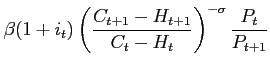
$\displaystyle \left(\frac{M_t}{P_t}\right)^{-\varphi}$	$\textstyle =$	$\displaystyle \frac{(C_t-H_t)^{-\sigma}}{\chi P_t}\left[ \frac{i_t}{1+i_t} \right]$	(10)
$\displaystyle \frac{W_t}{P_t}$	$\textstyle =$	$\displaystyle \frac{\kappa}{(1-\frac{1}{\eta})}N_t^\phi (C_t-H_t)^\sigma$	(11)

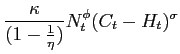
(9) is the familiar Keynes-Ramsey rule adapted to take into account of the consumption habit. In (10), the demand for money balances depends positively on consumption relative to habit and negatively on the nominal interest rate. Given the central bank's setting of the latter, (10) is completely recursive to the rest of the system describing our macro-model and will be ignored in the rest of the paper. 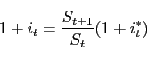(11) reflects the market power of households arising from their monopolistic supply of a differentiated factor input with elasticity $\eta$ . As labour becomes more homogeneous, this elasticity rises and the real wage households can command then falls.

Households can accumulate assets in the form of either home or foreign bonds. Uncovered interest rate parity then gives

$\begin{displaymath} 1+i_t=\frac{S_{t+1}}{S_{t}}(1+i_t^*) \end{displaymath}$

(12)

where

is the interest rate paid on nominal bonds denominated in foreign currency.

3.2 Firms

Competitive final goods firms use a continuum of non-traded intermediate goods according to a constant returns CES technology to produce aggregate output

$\begin{displaymath} Y_{t}=\left( \int_{0}^{1}Y_{t}(m)^{(\zeta -1)/\zeta }dm\right) ^{\zeta /(\zeta -1)} \end{displaymath}$

(13)

where $\zeta$ is the elasticity of substitution. This implies a set of demand equations for each intermediate good

with price $P_{Ht}(m)$ of the form

$\begin{displaymath} Y_{t}(m)=\left( \frac{P_{Ht}(m)}{P_{Ht}}\right) ^{-\zeta }Y_{t} \end{displaymath}$

(14)

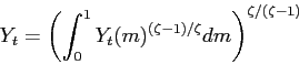
where $P_{Ht}=\left[ \int_0^1 P_{Ht}(m)^{1-\zeta} dm \right]^{ \frac{1}{1-\zeta}}$ . $P_{Ht}$ is an aggregate intermediate price index, but since final goods firms are competitive and the only inputs are intermediate goods, it is also the domestic price level.

In the intermediate goods sector each good is produced by a single firm using only differentiated labour with another constant returns CES technology:

$\begin{displaymath} Y_{t}(m)=A_{t}\left( \int_{0}^{1}N_{tm}(r)^{(\eta -1)/\eta }dr\right) ^{\eta /(\eta -1)} \end{displaymath}$

(15)

where $N_{tm}(r)$ is the labour input of type

by firm

and $A_{t}$ is an exogenous shock capturing shifts to trend total factor productivity (TFP) in this sector. Minimizing costs $\int_{0}^{1}W_{t}(r)N_{tm}(r)dr$ and aggregating over firms leads to the demand for labor as shown in (3). In a equilibrium of equal households and firms, all wages adjust to the same level $W_{t}$ and it follows that

$\begin{displaymath} Y_{t}=A_{t}N_{t} \end{displaymath}$

(16)

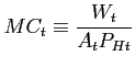
For later analysis it is useful to define the real marginal cost as the wage relative to domestic producer price. Using (11) and (16) this can be written as

$\displaystyle MC_{t} \equiv \frac{W_{t}}{A_{t}P_{Ht}}$

$\textstyle =$

$\displaystyle \frac{\kappa }{(1-\frac{1}{\eta })A_{t}}\left( \frac{Y_{t}}{A_{t}... ...) ^{\phi }(C_{t}-H_{t})^{\sigma }\left( \frac{P_{Ft}}{P_{Ht}}\right) ^{\omega }$

(17)

Now we assume that there is a probability of $1-\xi$ at each period that the price of each intermediate good is set optimally to $P_{Ht}^{0}(m)$ . If the price is not re-optimized, then it is indexed to last period's aggregate producer price inflation.¹⁴ With indexation parameter $\gamma \geq 0$ , this implies that successive prices with no reoptimization are given by $P_{Ht}^{0}(m),\,\,P_{Ht}^{0}(m)\left( \frac{P_{H,t+1}}{P_{Ht}}\right) ^{\gamma },\,\,P_{Ht}^{0}(m)\left( \frac{P_{H,t+2}}{P_{Ht}}\right) ^{\gamma },... \,\,\,$ . For each intermediate producer the objective is at time to choose $\{P_{Ht}(m)\}$ to maximize discounted profits

$\begin{displaymath} \mathcal{E}_{t}\sum_{k=0}^{\infty }\left(\frac{\xi}{1+i_t} \... ...t+k}}{P_{Ht}}\right) ^{\gamma }-\frac{W_{t+k}}{A_{t}} \right] \end{displaymath}$

(18)

given

(since firms are atomistic), subject to (14). The solution to this is

$\begin{displaymath} \mathcal{E}_{t}\sum_{k=0}^{\infty }\left(\frac{ \xi}{1+i_t} ... ...amma }-\frac{1}{ (1-1/\zeta) }\frac{W_{t+k}}{A_{t}}\right] =0 \end{displaymath}$

(19)

and by the law of large numbers the evolution of the price index is given by

$\begin{displaymath} P_{H,t+1}^{1-\zeta }=\xi \left( P_{Ht}\left( \frac{P_{Ht}}{P... ... ^{\gamma }\right) ^{1-\zeta }+(1-\xi )(P_{Ht}^{0})^{1-\zeta } \end{displaymath}$

(20)

3.3 The Equilibrium and the Trade Balance

In equilibrium, goods markets, money markets and the bond market all clear. Equating the supply and demand of the home consumer good and using (5) and the foreign counterpart of (6) we obtain

$\displaystyle Y_t$

$\textstyle =$

$\displaystyle C_{Ht}+C_{Ht}^*=\frac{P}{P_H} \left[(1-\omega) C+ \omega E C^* \right]$

(21)

Given interest rates

(expressed later in terms of a IFB rule) the money supply is fixed by the central banks to accommodate money demand. By Walras' Law we can dispense with the bond market equilibrium condition. Then a perfect foresight equilibrium is defined at

as sequences

, $C_{Ht}$ , $C_{Ft}$ , $P_{Ht}$ , $P_{Ft}$ ,

, $P_{Ht}^O$ , 12 foreign counterparts

, etc,

, and

, given past price indices and exogenous TFP processes. These 26 endogenous variables in total are given by 12 equations: (2), (5), (6), (7), (9), (10), (11), (19), (20), (21), and their foreign counterparts, and (8) and (12).

Combining the Keynes-Ramsey equations with the UIP condition we have that

$\begin{displaymath} \frac{P_{t}^{\ast }}{P_{t}}\left( \frac{C_{t}-hC_{t-1}}{C_{t... ...1}-hC_{t}}{C_{t+1}^{\ast }-hC_{t}^{\ast }}\right) ^{-\sigma } \end{displaymath}$

(22)

Let $z_{t}=\frac{S_{t}P_{t}^{\ast }}{P_{t}}\left( \frac{C_{t}-hC_{t-1}}{ C_{t}^{\ast }-hC_{t-1}^{\ast }}\right) ^{-\sigma }$ . Then (22) implies that $z_{t+1}=z_{t}$ . We consider a linearization in the vicinity of a symmetric steady state, $\bar{z}=1$ . From the transient nature of the shocks it follows that this steady state remains unchanged and hence $z_{t}=1$ in any stable rational expectations equilibrium. Therefore¹⁵

$\begin{displaymath} \left( \frac{C_{t}-hC_{t-1}}{C_{t}^{\ast }-hC_{t-1}^{\ast }}... ...) ^{-\sigma }=\frac{P_{t}}{S_{t}P_{t}^{\ast }}=\frac{1}{E_{t}} \end{displaymath}$

(23)

The model as it stands with habit persistence (), $\sigma >1$ and $\omega \in \lbrack 0,\frac{1}{2})$ exhibits net foreign asset dynamics. This can be shown by writing the trade balance $\mbox{TB}_{t}$ in the home bloc as exports minus imports denominated its own currency:

$\begin{displaymath} \mbox{TB}_{t}=P_{Ht}C_{Ht}^{\ast }-P_{Ft}C_{Ft}=\omega \left... ...t }-P_{t}C_{t}\right) =\omega P_{t}(E_{t}C_{t}^{\ast }-C_{t}) \end{displaymath}$

(24)

using (5) and (6), the law of one price $P_{Ht}=S_{t}P_{Ht}^{\ast }$ , and recalling the definition $E_{t}\equiv \frac{ S_{t}P_{t}^{\ast }}{P_{t}}$ . Therefore there are net foreign asset dynamics unless $C_{t}=E_{t}C_{t}^{\ast }$ . This is only compatible with (23) if either $\omega =\frac{1}{2}$ (no home bias), in which case $E_{t}=1$ , and we start off with balanced trade; or if $\sigma =1$ and

(no habit persistence).¹⁶

3.4 Linearization

We linearize around a baseline symmetric steady state in which consumption and prices in the two blocs are equal and constant. Then inflation is zero, $E_{t}=\bar{E}=1$ and hence from (24) trade is balanced. Output is then at its sticky-price, imperfectly competitive natural rate and from the Keynes-Ramsey condition (9) the nominal rate of interest is given by $\bar{\imath}=\frac{1}{\beta }-1$ . Now define all lower case variables (including $i_{t}$ ) as proportional deviations from this baseline steady state¹⁷. Home producer and consumer inflation are defined as $\pi _{Ht}\equiv\frac{P_{Ht}-P_{H,t-1}}{P_{H,t-1} }\simeq p_{Ht}-p_{H,t-1}$ and $\pi _{t}\equiv\frac{P_{t}-P_{t-1}}{P_{t-1} }\simeq p_{t}-p_{t-1}$ respectively. Similarly, define foreign producer inflation and consumer price inflation. Combining (19) and (20), we can eliminate $P_{Ht}^{0}$ to obtain in linearized form

$\begin{displaymath} \pi _{Ht}=\frac{\beta }{1+\beta \gamma }\mathcal{E}_{t}\pi _... ...1}+\frac{(1-\beta \xi )(1-\xi )}{(1+\beta \gamma )\xi }mc_{t} \end{displaymath}$

(25)

The linearized version of the real marginal cost for producers of intermediate goods in the home bloc, (17), is given by

$\begin{displaymath} mc_{t}=-(1+\phi )a_{t}+\frac{\sigma }{1-h}(c_{t}-hc_{t-1})+\phi y_{t}+\omega (s_{t}+p_{Ft}^{\ast }-p_{Ht}) \end{displaymath}$

(26)

The first term on the right-hand-side of (26) is a TFP shock. The second term is a risk-sharing effect: a rise in habit-adjusted consumption leads to an increase in the real wage (see (11)) and hence the marginal cost. The last term is a terms of trade effect, which implies that marginal costs falls if the terms of trade, $p_{Ht}-s_{t}-p_{Ft}^{\ast }$ in linearized form, rises.

Linearizing the remaining equations (8), (9), (12), (21) and (23) yields¹⁸

$\displaystyle \pi_t-\pi^*_t$	$\textstyle =$	$\displaystyle 2\omega(s_t-s_{t-1})+(1-2\omega)(\pi_{Ht}-\pi^*_{Ft})$	(27)
$\displaystyle c_t-\frac{h}{1+h}c_{t-1}$	$\textstyle =$	$\displaystyle \frac{1}{1+h}\mathcal{E}_t c_{t+1}-\frac{1-h}{(1+h)\sigma}(i_t-\mathcal{E}_t \pi_{t+1})$	(28)
$\displaystyle \mathcal{E}_t\Delta s_{t+1}$	$\textstyle =$	$\displaystyle i_t-i^*_t$	(29)
$\displaystyle y_t$	$\textstyle =$	$\displaystyle (1-\omega)c_t+\gamma c^_t-2\omega(1-\omega)(p_{Ht}-s_t-p^_{Ft})$	(30)
$\displaystyle \sigma(c^_t-c_t-h(c^_{t-1}-c_{t-1}))$	$\textstyle =$	$\displaystyle -e_t=(1-2\omega)(p_{Ht}-s_t-p^*_{Ft})$	(31)

Note that (30) and its foreign counterpart imply that $y_{t}+y_{t}^{\ast }=c_{t}+c_{t}^{\ast }$ . Also note that for the case when there is no home bias, $\omega =1/2$ . Then (27) reduces to relative purchasing power parity for consumer price inflation.

Turning to spillover effects in our linearized form of the model, consider the case of no home bias. Then from (30) and (26) we obtain

$\begin{displaymath} mc_{t}=\frac{\sigma }{2(1-h)}\left[ y_{t}-hy_{t-1}+y_{t}^{\a... ...ht] +\phi y_{t}+\frac{1}{2}\left[ y_{t}-y_{t}^{\ast } \right] \end{displaymath}$

(32)

It follows that the elasticity of marginal cost for intermediate goods home producers with respect to domestic and foreign current output, given output at time

, are given by $\kappa \equiv \frac{\partial mc_{t}}{\partial y_{t}}$ and $\kappa _{0}\equiv \frac{\partial mc_{t}}{\partial y_{t}^{\ast }}$ where

$\displaystyle \kappa$

$\textstyle =$

$\displaystyle \frac{\sigma}{2(1-h)}+\frac{1}{2}+\phi\,; \quad \quad \kappa_0=\frac{\sigma}{2(1-h)}-\frac{1}{2}$

(33)

(33) indicates that the risk-sharing effect exceeds the terms of trade effect and there is positive spillover from output onto the marginal cost of the second bloc--implying a negative spillover on output--iff $\frac{ \sigma }{1-h}>1$ in the short-run (i.e., given output in period

). ¹⁹Iff $\frac{\sigma }{1-h}=1$ , the risk-sharing and terms of trade effect cancel and there are no spillover effects. Empirical estimates discussed in Appendix C suggest that $\sigma >1,$ so under this calibration in our model spillover effects on output are negative. The effect of introducing habit is to enhance the risk-sharing effect and enhance these negative short-run spillovers.

3.5 Sum and Difference Systems

Since the economies are symmetric, the easiest way of analyzing them is to use the sum and difference systems, as introduced by Aoki (1981). We denote all sums of home and foreign variables with the superscript , while we denote differences by . The first thing to note when inspecting the equations above is that the sum system is independent of home bias, and can be written as

$\displaystyle \pi_t^S$	$\textstyle =$	$\displaystyle \frac{\beta}{1+\beta\gamma}\mathcal{E}_t\pi_{t+1}^S+\frac{\gamma}{1+\beta\gamma} \pi_{t-1}^S$
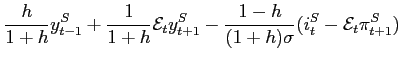
	$\textstyle +$	$\displaystyle \frac{(1-\beta\xi)(1-\xi)}{(1+\beta\gamma)\xi}[(\phi+\frac{\sigma}{1-h}) y_t^S-\frac{\sigma h}{1-h}y_{t-1}^S-(1+\phi)a_t^S]$	(34)
$\displaystyle y^S_t$	$\textstyle =$	$\displaystyle \frac{h}{1+h}y^S_{t-1}+\frac{1}{1+h}\mathcal{E}_ty^S_{t+1}-\frac{1-h}{(1+h)\sigma} (i_t^S-\mathcal{E}_t\pi^S_{t+1})$	(35)

where $\pi^S=\pi_H+\pi_F^*$ ,

, and we note that $\pi_H+\pi_F^*=\pi+\pi^*$ .

However the difference system does depend on the home bias parameter, $\omega$ , Writing $\pi^D=\pi_H-\pi_F^*$ , , etc., it can be written as

$\displaystyle \pi^D_t$	$\textstyle =$	$\displaystyle \frac{\beta}{1+\beta\gamma}\mathcal{E}_t\pi_{t+1}^D+\frac{\gamma}{1+\beta\gamma} \pi_{t-1}^D+\frac{(1-\beta\xi)(1-\xi)}{(1+\beta\gamma)\xi}mc^D_t$	(36)
$\displaystyle mc_t^D$	$\textstyle =$	$\displaystyle -(1+\phi)a^D_t+\frac{\sigma}{1-h}(c^D_t-hc^D_{t-1})+\phi y^D_t+2{\bf\omega} (s_t+p^*_{Ft}-p_{Ht})$	(37)
$\displaystyle c^D_t$	$\textstyle =$	$\displaystyle hc^D_{t-1}+\frac{(2\omega-1)}{\sigma}(p_{Ht}-s_t-p^*_{Ft})$	(38)
$\displaystyle y^D_t$	$\textstyle =$	$\displaystyle (1-2\omega)c^D_t-4\omega(1-\omega)(p_{Ht}-s_t-p^*_{Ft})$	(39)
$\displaystyle \mathcal{E}_t\Delta s_{t+1}$	$\textstyle =$	$\displaystyle i^D_t$	(40)

For the case of no home consumption bias ( $\omega =\frac{1}{2}$ ) taking first differences of (39) and using (40) we have

$\begin{displaymath} \mathcal{E}_{t}y_{t+1}^{D}-y_{t}^{D}=i_{t}^{D}-\mathcal{E}_{t}\pi _{t+1}^{D} \end{displaymath}$

(41)

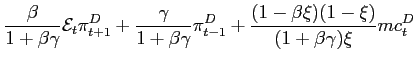
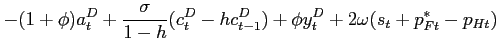
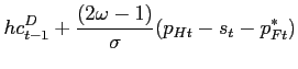
In addition, when there is no home bias, the remainder of the difference system reduces to

$\begin{displaymath} \pi _{t}^{D}=\frac{\beta }{1+\beta \gamma }\mathcal{E}_{t}\p... ...-\xi )}{ (1+\beta \gamma )\xi }(1+\phi )(y_{t}^{D}-a_{t}^{D}) \end{displaymath}$

(42)

Note, as with other models of the same New Keynesian genre, there is a long-run inflation-unemployment trade-off.²⁰

The sum and difference systems can now be set up in state-space form given the nominal interest rate rule. This Aoki decomposition enables us to decompose the open economy into two decoupled dynamic systems; the sum system, that captures the properties of a closed world economy, and a difference system that instead portrays the open-economy case. In principle, we could close the model with a number of different Taylor-type rules and also, given a policymaker's objective function, with optimal rules for coordinated or independent policies. Here we choose to focus uniquely on IFB rules that feedback exclusively on expected inflation. Before doing so, in the next section we first offer answers to the more general question of why is it interesting to look at simple rules. We also discuss why, within the broader class of simple rules, we consider non-optimal simple rules rather than simple rules which are optimal within the constraints defining their Taylor form of simplicity.

4 Designing and Implementing Optimal Policy

4.1 Formulating the Optimal Rule

The analysis of IFB rules set out in the next section contributes to a large literature on monetary policy rules that focusses primarily on the properties of these non-optimizing simple rules, thereby neglecting the possibility that central banks set monetary conditions by means of some explicit optimizing procedure. This approach has been criticized by Svensson (2001, 2003), and in this section we attempt to address his critique. We start with a commonly used objective function at time for the home bloc of the form

$\begin{displaymath} \Omega _{0}=-\mathcal{E}_{0}\sum_{t=0}^{\infty }\beta ^{t}[\pi _{t}^{2}+\alpha _{y}(y_{t}-k)^{2}+\alpha _{i}i_{t}^{2}] \end{displaymath}$

(43)

with an analogous expression for the foreign bloc. The term k indicates an ambitious output target which captures the distortion in our model arising from imperfect competition. The last term captures the policymaker's concern for deviations of the nominal interest rate from the natural rate $\bar{\imath}=\frac{1}{\beta }-1$ . Recently, this `pragmatic' approach to rationalizing policy objectives has been replaced by a completely coherent approach that bases the policymaker's objectives on those of the representative household. CGG (2002) and BB pursue the latter course, and the form (43) with

corresponds loosely to their quadratic approximation to the utility of the representative household. ²¹

Our linearized model can be expressed in state-space form as

$\begin{displaymath} \left[ \begin{array}{l} z_{t+1} \ \mathcal{E}_t x_{ t+1} \... ...hsf{B}\left[ \begin{array}{l} i_t \ i_t^* \end{array}\right] \end{displaymath}$

(44)

where $\mathsf{z}_t=[k, a_{t-1}, a_{t-1}^*, y_{t-1}, y_{t-1}^*, \pi_{H(t-1)}, \pi_{F (t-1)}^*]$ is a vector of predetermined variables and $\mathsf{x}_t=[y_{t}, y_{t}^*, \pi_{Ht}, \pi_{F t}^*]$ is a vector of non-predetermined variables. A, and B are matrices with time-invariant coefficients. In our deterministic perfect foresight model, transient shocks are unanticipated and follow an exogenous process such as $a_t=\varrho a_{t-1}; a^*_t=\varrho^* a_{t-1}^*$ , $\varrho, \varrho \in [0,1)$ , with

and

given. Remaining predetermined variables begin at their steady state values; i.e.,

, etc.²² Then the optimization problem for a world social planner is to maximize $a\Omega_O +(1-a) \Omega_0^*$ subject to (44) (where $\Omega_0^*$ is analogously defined for the foreign bloc) is set out in general form in Appendix A.²³The optimal rule given by this problem takes the `history-dependent' form

$\begin{displaymath} \left[ \begin{array}{l} i_t \ i^*_t \end{array}\right]=D_1z_t+D_2C_{21} \sum_{\tau=1}^{t}(C_{22})^{\tau-1}z_{t-\tau} \end{displaymath}$

(45)

say, where

, $C_{21}$ and $C_{22}$ are segments of partitioned matrices defined in Appendix A. (45) can be decomposed into two parts. By including a relationship $k_{t+1}=k_t=k$ (a constant) in the state-space representation we can extract an open-loop component of policy that results from the inclusion of an ambitious output target in (43). (45) then decomposes into open-loop trajectories for the nominal interest rate plus a feedback that depends on the initial TFP shocks

and

4.2 Implementing the Optimal Policy and Simple Rules

The optimal cooperative policy then consists of trajectories for nominal interest rates that would be followed in the absence of initial shocks to TFP (or, in a stochastic setting, in the absence of random shocks) and a reaction function consisting of a feedback on the lagged predetermined variables with geometrically declining weights with lags extending back to time , the time of the formulation and announcement of the policy. Together these components constitute an explicit instrument rule. ²⁴As is well-known, there are two fundamental problems with implementing such a rule. First it is time-inconsistent: having announced the policy at time , at any time there emerges an incentive for the social planner to redesign both open-loop and feedback components of policy. Second, the cooperative policy is not a Nash equilibrium so there exists at any time, including , an incentive to renege and adopt a policy that is the best response to that of the other bloc.

One way of implementing the optimal policy that addresses both the time-inconsistency and cooperation problems is to design objective functions for the two blocs that do not coincide with the true welfare. The aim of the exercise is to choose this design, or `regime', so that if the two blocs independently optimize in a discretionary fashion, then in a non-cooperative time-consistent equilibrium the optimal policy will be implemented. Thus BB, in addressing the cooperation problem, force the central banks to be `inward-looking' in the sense that their loss function only includes domestic target (e.g., producer inflation rather than consumer inflation which implies an exchange rate target). Svensson and Woodford (2003) adopt this modified loss function approach to the time-inconsistency problem for a closed economy. The idea of modifying loss functions so that players in a game have the `wrong' welfare criteria is, of course, not new and is the basis of Rogoff-delegation and Walsh contracts. To a greater or lesser extent all these solutions are susceptible to the critique by McCallum (1995) of Walsh contracts, that they do not solve either the credibility or the coordination problem, but ``merely relocate'' them to demonstrating the commitment of the policymakers to their modified loss functions.

A second way of implementing optimal policy is to build up a reputation for commitment to both the second bloc and to the private sector. In a more realistic incomplete information setting where policymakers' objectives are not known to the public, but policy rules can be observed, the public can learn about the rule by observing the relevant data and applying standard econometric techniques. In principle this should be possible for rules of the form (45), but the New Keynesian features of the model (namely output and inflation persistence) make it particularly complex. This highlights the importance of rules being simple in the sense that the instrument is constrained to feed back on a limited number of variables and their lags such as in a Taylor rule, or their forecasts as in IFB rules.

As well as being more easily verifiable, simple rules may have other advantages. As shown in Currie and Levine (1993) and Tetlow and von zur Muehlen (2001), it is easier to learn about simple rules that (by definition) feed back on a limited selection of easily verifiable macro-variables, than to learn about complex optimal rules such as (45) . Taking this ability to learn into account, simple rules may then outperform their optimal counterparts. Finally it has been suggested that simple rules may be robust with respect to modelling errors (LWW, Taylor (1999)).

Simple rules can be designed to approximate the optimal rule by choosing the feedback parameters so as to maximize an objective function of the form (43). However the simplicity constraint means that the optimal simple rule is not certainty equivalent, unlike the optimal rule unconstrained to be simple. This means that if at time we designed a optimal simple rule of a particular form for our model above, optimal feedback parameters would depend on the transient shocks to TFPs, $a_{0}$ and $a_{0}^{\ast }$ and, in a stochastic setting, on the variance-covariance matrix of white noise disturbances in the stochastic process defining these shocks.²⁵ Then rules that perform well, in the sense of achieving a welfare outcome close to that of the optimal rule, under one assumed set of initial displacements and covariance matrix may well lack robustness in that they may perform badly under a different set of assumptions. However some structures of simple rule may be more robust than others.²⁶

Defining what we mean by the optimal simple rule is then problematic. The literature on determinacy, to which our paper contributes, has a more modest objective of providing guidelines to policymakers in the form of simple criteria for avoiding very bad outcomes that lead to multiple equilibria or explosive behaviour. In our set-up, these guidelines focus on the choice of feedback, interest rate smoothing and feedback horizon parameters. In the following section we pursue this research objective by looking at how such guidelines are affected when we proceed from the closed to the open economy and by the degree of openness in the latter.

5 The Stability and Determinacy of IFB Rules

This section studies two particular forms of simple rule, IFB rules either of the form

$\begin{displaymath} i_t=\rho i_{t-1}+\theta(1-\rho)\mathcal{E}_t \pi_{t+j} \end{displaymath}$

(46)

where $j \ge 0$ is the forecast horizon, which is a feedback on consumer price inflation, or of the form

$\begin{displaymath} i_t=\rho i_{t-1}+\theta(1-\rho)\mathcal{E}_t \pi_{H t+j} \end{displaymath}$

(47)

which is a feedback on producer price inflation. Both rules are in deviation form about some long-run zero-inflation steady state and could represent the feedback component of monetary policy that complements a (possibly optimal) open-loop trajectory designed as in the previous section. We assume that the foreign bloc has a similar rule with the same parameters and forecast horizon.

With rules (46) and (47), policymakers set the nominal interest rate so as to respond to deviations of the inflation term from target. In addition, policymakers smooth rates, in line with the idea that central banks adjust the short-term nominal interest rate only partially towards the long-run inflation target, which is set to zero for simplicity in our set-up.²⁷ The parameter $\rho \in \lbrack 0,1)$ measures the degree of interest rate smoothing. is the feedback horizon of the central bank. When , the central bank feeds back from current dated variables only. When , the central bank feeds back instead from deviations of forecasts of variables from target. This is a proxy for actual policy in inflation targeting countries that apparently respond to deviations of current inflation from its short or medium forecast (see Batini and Nelson (2001)). Finally, $\theta >0$ is the feedback parameter: the larger is $\theta$ , the faster is the pace at which the central bank acts to eliminate the gap between expected inflation and its target value. We now show that, for given degrees of interest rate smoothing $\rho$ , the stabilizing characteristics of these rules depend both on the magnitude of $\theta$ and the length of the feedback horizon .

5.1 Conditions for the Uniqueness and Stability

To understand better how the precise combination of the pair $(j,\theta )$ , IFB rules can lead the economy into instability or indeterminacy consider the model economy (44) with interest rate rules of the form (46) or (47) with . Shocks to TFP are exogenous stable processes and play no part in the stability analysis. Furthermore we are only concerned with the feedback component of policy. We therefore set $k=a_{t}=a_{t}^{\ast }=0$ in (44). Write the IFB rules in the form²⁸

$\begin{displaymath} \left[ \begin{array}{l} i_{t} \ i_{t}^{\ast } \end{array}\... ...array}{l} \mathsf{z}_{t} \ \mathsf{x}_{t} \end{array}\right] \end{displaymath}$

(48)

where $\mathsf{z}_{t}=[y_{t-1},y_{t-1}^{\ast },\pi _{H(t-1)},\pi _{F(t-1)}^{\ast },i_{t-1},i_{t-1}^{\ast }]$ and $\mathsf{x} _{t}=[y_{t},y_{t}^{\ast },\pi _{Ht},\pi _{Ft}^{\ast }]$ to give the system (44) under control as

$\begin{displaymath} \left[ \begin{array}{l} \mathsf{z}_{t+1} \ \mathcal{E}_{t}... ...array}{l} \mathsf{z}_{t} \ \mathsf{x}_{t} \end{array}\right] \end{displaymath}$

(49)

The condition for a stable and unique equilibrium depends on the magnitude of the eigenvalues of the matrix . If the number of eigenvalues outside the unit circle is equal to the number of non-predetermined variables, the system has a unique equilibrium which is also stable with saddle-path where . (See Blanchard and Kahn (1980); Currie and Levine (1993)). In our model under control, with , there are 4 non-predetermined variables in total, 2 each for the sum and difference systems and 6 predetermined variables in total, 3 each for the sum and difference systems. Instability occurs when the number of eigenvalues of outside the unit circle is larger than the number of non-predetermined variables. This implies that when the economy is pushed off its steady state following a shock, it cannot ever converge back to it, but rather finishes up with explosive inflation dynamics (hyperinflation or hyperdeflation).

By contrast, indeterminacy occurs when the number of eigenvalues of outside the unit circle is smaller than the number of non-predetermined variables. Put simply, this implies that when a shock displaces the economy from its steady state, there are many possible paths leading back to equilibrium, i.e. there are multiple well-behaved rational expectations solutions to the model economy. With forward-looking rules this can happen when policymakers respond to private sector's inflation expectations and these in turn are driven by non-fundamental exogenous random shocks (i.e. not based on preferences or technology), usually referred to as `sunspots'. If policymakers set the coefficients of the rule so that this accommodates such expectations, the latter become self-fulfilling. Then the rule is unable to uniquely pin down the behavior of one or more real and/or nominal variables, making many different paths compatible with equilibrium (see Kerr and King (1996); Chari et al. (1998); CGG (2000); Carlstrom and Fuerst (1999) and Carlstrom and Fuerst (2000); Svensson and Woodford (1999); and Woodford (2000)). The fact that the rule itself may introduce indeterminacy and generate so called `sunspot equilibria' is of interest because sunspot fluctuations - i.e., persistent movements in inflation and output that materialize even in the absence of shocks to preferences or technology - are typically welfare-reducing and can potentially be quite large.

In order to gain insight into the stabilizing properties of IFB rules, following Batini and Pearlman (2002) we analyze their performance by using root locus analysis, a method that we borrow from the control engineering literature. Appendix B outlines how this method works. Use of this method allows us to identify analytically the range of stabilizing parameters $(j,\theta )$ in our sticky-price/sticky-inflation models before indeterminacy sets in. The method produces geometrical representations that show how system eigenvalues change as a function of the change in any parameter in the system. In our particular case we are interested in detecting how the characteristic roots of the model economy evolve as we vary the inflation feedback parameter $\theta$ , for given forecast horizons in the policy rule. As the conditions for stability and determinacy of the model hinge on the value of these roots, from these diagrams we can infer which regions of the $\left( j,\theta \right)$ parameter space are associated with unique and well-behaved REE. Since we condition on increasingly distant forecast horizons in the policy rule, the method entails deriving a separate diagram for each value of . However, in the majority of cases a clear pattern emerges quickly, so in what follows we only draw these diagrams at most for = 0, 1,...,4.

In the following subsections, we use the Aoki method to analyze separately the sum and difference systems of two symmetric blocs pursuing symmetric IFB rules of the form (46) or (47). The results for the sum system can be thought of as applying to a closed economy. For open economies both sum and difference systems must be saddle-path stable for a stable and unique equilibrium. As previously mentioned, the central banks'choice of responding to consumer or price inflation as well as the existence of a home bias in consumption patterns are all irrelevant in the case of the sum system. In the case of the difference system this is no longer true, and so we investigate changes to these assumptions separately for that case.

5.2 The Sum System

The sum form of the IFB rule is given by

$\begin{displaymath} i_{t}^{S}=\rho i_{t-1}^{S}+\theta (1-\rho )\mathcal{E}_{t}\pi _{t+j}^{S} \end{displaymath}$

(50)

Let

be the forward operator. Taking z-transforms of (34) and (50), the characteristic equation for the sum system is given by:

		$\displaystyle (z-\rho )[(z-1)(z-h)(\beta z-1)(z-\gamma )-\frac{\lambda }{\mu }z^{2}(\phi z+\mu (z-h))]$
	$\textstyle +$	$\displaystyle \frac{\lambda \theta }{\mu }(1-\rho )(\phi z+\mu (z-h))z^{j+2}=0$	(51)

where we have defined

$\begin{displaymath} \lambda \equiv \frac{(1-\beta \xi )(1-\xi )}{\xi }\,;\quad \mu \equiv \frac{ \sigma }{1-h} \end{displaymath}$

(52)

Equation (51) shows that the minimal state-space form of the sum system has dimension $\max{(5, j+3)}$ . Recalling that there are 3 predetermined variables in each of the sum and difference systems, it follows that the saddle-path condition for a unique stable rational expectations solution in the general version of our model is that the number of stable roots (i.e., roots inside the unit circle of the complex plane) is 3 and the number of unstable roots is $\max{(2, j)}$ .

To identify values of $(j,\theta )$ that involve exactly three roots of equation (51) we use the root locus technique. In particular, this technique can help us uncover how the range of values of $\theta$ that are consistent with determinacy changes as the feedback horizon changes. The root locus technique provides topological proofs of our main results (Appendix B describes this technique in detail). The technique involves starting from a polynomial equation and using a set of topological theorems to track the equation's roots as parameters in the system vary. The locus describing the evolution of the roots when parameters change is called the `root locus'. In our analysis here, the polynomial equation is the characteristic equation (51), and we use the technique to graph the locus of $\left( \theta ,z\right)$ pairs that traces how the roots change as $\theta$ varies between 0 and $\infty$ . Other parameters in the system, including the feedback horizon parameter in the IFB rule, are kept constant. So to plot root loci for different feedback horizon we have to generate separate charts, each conditioning on a different horizon assumption. Each chart shows the complex plane (indicated by the solid thin line),²⁹ the unit circle (indicated by the dashed line), and the root locus tracking zeroes of equation (51) as $\theta$ varies between 0 and $\infty$ (indicated by the solid bold line). The arrows indicate the direction of the arms of the root locus as $\theta$ increases. Throughout we experiment with both a `higher' and a `lower' $\frac {\lambda }{\mu }$ , as defined in (52). The economic interpretation of these cases is as follows: from the definitions in (52), the high $\frac {\lambda }{\mu }$ case corresponds to low $\xi$ (i.e., more flexible prices) and low $\frac{ \sigma }{1-h}$ . From section 3.4 we have seen that the latter implies small spillover effects and hence low interdependence between the two blocs. Hence in the high $\frac {\lambda }{\mu }$ case, prices are relatively flexible and interdependence not as strong when compared with the low $\frac {\lambda }{\mu }$ case.

The term inside the square brackets in equation (51) corresponds to no nominal interest rate policy at all. With no policy rule in place, rule (46) or (47) is switched off and so the lagged term $i_{t-1}$ disappears from our model; the system now requires exactly two stable roots for determinacy. Figure 1 plots the root locus in this case. Since with no policy $\theta$ is set to 0, the root locus is just a set of dots: namely, the roots of equation (51) when $\theta =0$ . Note that depending on the value of $\lambda /\mu$ , the position of these roots varies, and in the flexible price, low independence case where $\frac {\lambda }{\mu }$ is high, there are complex roots indicating oscillatory dynamics.³⁰ The diagram shows that there are too many stable roots in both cases (i.e. 3 instead of 2), which implies that with no monetary policy there will always be indeterminacy in the sum system.

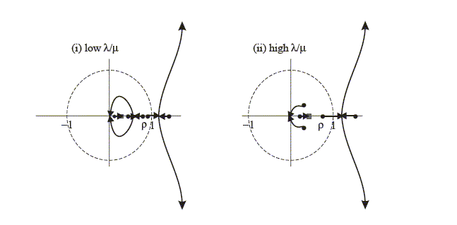
Figure 1: Possible position of zeroes when $\theta =0$

$Figure 1 plots the root locus for two cases: (i) low $\lambda/\mu$, and (i) high $\lambda/\mu$. In both cases, the x-axis is real, the y-axis is imaginary, and there is a (dashed) unit circle that intersects the x-axis at (x,y)=(-1,0) and (x,y)=(1,0), which are both labeled. In (i), four roots are plotted, all on the x-axis: three lie between x=0 and x=1, and one lies at about x=1.5. In (ii), four roots are plotted. Two are on the x-axis, with x=1/3 and x=1.8 (approximately). The other two are at approximately (0.5, +1/3) and (0.5, -1/3).$

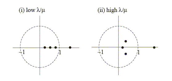
If the nominal interest rate rule is switched on and now feeds back on current rather than expected inflation, i.e. = 0, then the root locus technique yields a pattern of zeros as depicted in Figure 2. Interest rate smoothing brings about a lag in the short-term nominal interest rate and so means that the system is stable if it has exactly three stable roots (as we now have three predetermined variables in the system). The figure illustrates that if $\theta$ is sufficiently large, one arm of the root locus starting originally at $\rho$ exits the unit circle, turning one root from stable to unstable so that there are now three - as required - instead of four stable roots and the system has a determinate equilibrium. As $\theta\rightarrow\infty$ , there are roots at $\pm i \infty$ , two roots at , and one at $\mu h/(\phi + \mu)$ , the latter shown as a square.

Figure 2: Position of zeroes as $\theta$ changes using current inflation

Figure 2 duplicates the graphs in Figure 1, adding arrows depicting movements in roots when a nominal interest rate rule is switched on with $j=0$. In (i), two stable roots have arrows moving towards zero, with paths containing either positive or negative imaginary parts. And, on the right-hand side, a vertical line bulges to the left, intersecting the x-axis at x>1; and additional roots have arrows denoting their movement. In (ii), the two roots with imaginary parts have arrows curving toward zero; and (ii) has a similar vertical line to (i).

Note that when $\theta =z=1$ , the characteristic equation has the value 0, confirming that the branch of the root locus moving away from $z=\rho$ crosses the unit circle at a value $\theta =1$ . Thus we conclude that for a rule feeding back on current inflation the sum system exhibits determinacy if and only if $\theta >1$ . For higher values of $j \ge 1$ we can draw the sequence of root locus diagrams shown in Figures 3-6, and so confirm the well-known `Taylor Principle' that interest rates need to react to inflation with a feedback greater than unity. However for $j \ge 1$ our diagrams show that an arm of the root locus re-enters the unit circle for some high $\theta >1$ and indeterminacy re-emerges. Therefore $\theta >1$ is necessary but not sufficient for stability and determinacy. Our results up to this point are summarized in proposition 1 below.

Figure 3: Position of zeroes as $\theta$ changes: 1-period ahead expected inflation

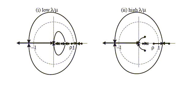
Figure 3 duplicates the graphs in Figure 1, adding arrows depicting movements in roots when a nominal interest rate rule is switched on with $j=1$. In (i), two stable roots have arrows moving towards zero, with paths containing either positive or negative imaginary parts. The largest stable root moves along the x-axis to a value >1, where that root and the unstable root curve outside the unit circle to a value of approximately (-1.3, 0). In (ii), the two roots with imaginary parts have arrows curving toward zero; and the two roots without imaginary parts behave like the two largest roots in (i).

Figure 4: Position of zeroes as $\theta$ changes: 2-period ahead expected inflation

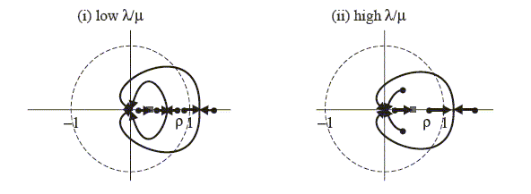
Figure 4 duplicates the graphs in Figure 1, adding arrows depicting movements in roots when a nominal interest rate rule is switched on with $j=2$. Both (i) and (ii) appear as in Figure 3, but with the outer paths entering the unit circle at about (0.8, +/-0.5). then briefly looping through the NW and SW quadrants to arrive at the origin.

Figure 5: Position of zeroes as $\theta$ changes: 3-period ahead expected inflation

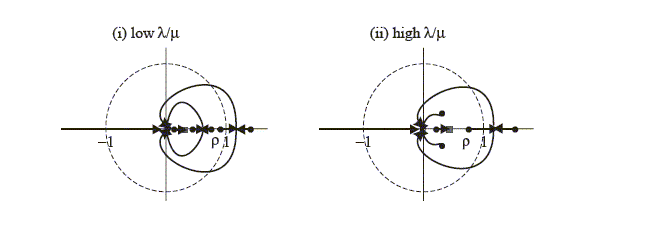
Figure 5 duplicates the graphs in Figure 1, adding arrows depicting movements in roots when a nominal interest rate rule is switched on with $j=3$. Figure 5 is visually very similar to Figure 4.

Figure 6: Position of zeroes as $\theta$ changes: 4-period ahead expected inflation

Figure 6 duplicates the graphs in Figure 1, adding arrows depicting movements in roots when a nominal interest rate rule is switched on with $j=4$. Figure 6 is visually very similar to Figure 4, but, for each of (i) and (ii), has vertical arrows entering the unit circle in the NW and SW quadrants and curving to the origin.

Proposition 1: In the sum system, for a rule feeding back on current inflation (

), $\theta >1$ is a necessary and sufficient condition for stability and determinacy. For higher feedback horizons ( $j \ge 1$ ), $\theta >1$ is a necessary but not sufficient condition for stability and determinacy.

When the rule starts responding to inflation expectations at longer horizons ( $\geq$ 1), self-fulfilling inflationary expectations and sunspot equilibria are once again possible as $\theta$ becomes too large. These manifest themselves as soon as the arms of the root locus that were outside the unit circle when $\theta$ = 0 and for small values of $\theta$ start entering the unit circle as $\theta$ increases. Let $\theta ^{S}(j)$ be the upper critical value of $\theta$ for the sum system for a feedback horizon . Figure 3 shows that for the case , i.e. one-quarter ahead forecasts which corresponds to a case studied by CGG (2000), indeterminacy occurs when this portion of the root locus enters the unit circle at .³¹ The critical upper value for $\theta =\theta ^{S}(1)$ when this occurs is obtained by substituting and into the characteristic equation (51) to obtain:

$\begin{displaymath} \theta ^{S}(1)=\frac{1+\rho }{1-\rho }\left[ 1+\frac{2(1+h)(1+\beta )(1+\gamma )\mu }{\lambda (\phi +\mu (1+h))}\right] \end{displaymath}$

(53)

One important thing to note looking at this expression is that the greater is the degree of smoothing captured by the parameter $\rho$ in the interest rate rule, the larger the maximum permissible value of $\theta$ before indeterminacy sets in. For $j\geq 2$ , Figures 4-6 show that indeterminacy occurs when the root locus enters the unit circle at $z=cos(\psi )+isin(\psi )$ for some $\psi \in (0,\frac{\pi }{2})$ . In this case, the threshold $\theta ^{S}(j)$ for $j\geq 2$ must be found numerically. Given , write the characteristic equation as

$\begin{displaymath} \sum_{k=1}^{max(5,J+3)}a_{k}z^{k}=0 \end{displaymath}$

(54)

where some of the $a_{k}$ are dependent on $\theta .$ The root locus meets the unit circle at $z=cos(\psi )+isin(\psi )$ . Using De Moivre's theorem $z^{k}=cos(k\psi )+isin(k\psi )$ and equating real and imaginary parts we arrive at two equations

$\displaystyle \sum_{k=1}^{max(5,j+3)} a_k(\theta) cos (k \psi)=0\,; \quad \quad \sum_{k=1}^{max(5,j+3)} a_k(\theta) sin (k \psi)=0$

(55)

which can be solved numerically for $\theta$ and $\psi$ .³²

As well as locating an upper threshold $\theta =\theta ^{S}(j)$ , an even more significant result concerning indeterminacy emerges from Figures 4, 5 and 6 for $j\geq 2$ . These have been drawn in such a way that the two rightmost poles of the root locus are joined by straight lines that meet outside the unit circle. The implication is that for some values of $\theta >1$ , these yield unstable roots of the system, and therefore the system will have exactly three stable roots which is what is required for determinacy. (Note that if the arms of the root locus from $\infty$ cross the unit circle before these latter meet, then there may anyway be too many stable roots). However, for a lower value of $\rho$ it could happen that rather than meeting to the right of , the two arms instead meet to the left of , that is inside the unit circle and then remain within it, as in figure 7. This would imply that for all $\theta$ there are always more than three stable roots, which would entail, in turn, indeterminacy for all values of $\theta$ . We therefore conclude that there is determinacy for $\theta$ slightly greater than 1 if the root locus passes through from the left, as in figures 3-6. Conversely, there is indeterminacy for all $\theta$ if the root locus passes through from the right, as in Figure 7; this equivalent to the condition $\partial z/\partial \theta <0$ at . We now use this topological argument to prove the following proposition:
Proposition 2: Whatever the combination of parameter values, there is always some lead $J^{S}$ given by (56) below such that for $j>J^{S}$ there is indeterminacy for all values of $\theta$ .

Proof: Write (51) as $f+\theta g=0$ . Taking derivatives with respect to $\theta$ , and evaluating at $\theta=1, z=1$ yields $[f^{\prime}(1)+g^{\prime}(1)]\frac{\partial z}{ \partial \theta}+g(1)=0$ . By inspection , so that the root locus crosses from the right if $f^{\prime}(1)+g^{\prime}(1)>0$ . Substituting from (51), this is a requirement that $(1-\rho)(1-h)(\beta-1)(1-\gamma)-\lambda/\mu(\phi +\mu-\mu h)+j(1-\rho)\lambda/\mu(\phi +\mu-\mu h)>0$ and $g^{\prime}(1)>0$ . Since guarantees the latter condition, there is always indeterminacy if

$\begin{displaymath} j>J^S=\frac{1}{1-\rho}+\frac{(1-\beta)(1-\gamma)\sigma}{\lambda(\phi+\sigma)} \end{displaymath}$

(56)

This completes the proof. $\,\,\,\Box$

Figure 7: Position of zeros as $\theta$ changes: 3-period ahead expected inflation, and low $\rho$

$Figure 7 duplicates the graphs in Figure 1, adding arrows depicting movements in roots when a nominal interest rate rule is switched on with $j=3$ and low $\rho$. Figure 7 is visually very similar to Figure 4, except that, for each of (i) and (ii), the outer looping arrows are within the unit circle.$

The value of $\rho$ is crucial in determining the critical value of the lead beyond which indeterminacy sets in. The lower $\rho$ , the lower the maximum-permitted inflation horizon the central bank can respond to, and hence, the larger the region of indeterminacy under IFB rules.

5.3 The Difference System

In this section we analyze the effect of the IFB rule in the difference system. We shall see that, in this case, there are important differences in the conditions for determinacy depending on (i) whether the central banks react to producer or consumer price inflation and on (ii) the degree of openness of the two economies (as captured by the parameter $\omega$ ). We start by considering the case of complete integration (i.e. $\omega =\frac{1}{2}$ and no home bias), looking first at IFB rules based on producer price inflation and then at IFB rules based on consumer price inflation. Then we consider the case when there is home bias, however restricting ourselves to the case of no habit formation () and a unit elasticity of substitution in the utility function ( $\sigma =1$ ). These more restrictive assumptions imply no foreign asset dynamics about a balanced trade steady state (since trade is always balanced), as when we assumed no home bias. Without these restrictions we need to address the well-known problems associated with Ramsey consumers in open economies (see, for example, Schmitt-Grohe and Uribe, 2001).³³

5.3.1 No Home Bias and IFB Rules Based on Producer Price Inflation

With interest rates feeding back on producer price inflation, the IFB rule in difference form is given by

$\begin{displaymath} i_{t}^{D}=\rho i_{t-1}^{D}+\theta (1-\rho )\mathcal{E}_{t}\pi _{t+j}^{D} \end{displaymath}$

(57)

Taking

-transforms of (57), (39) and (42), it is now easy to show that for the difference system the characteristic equation reduces to

$\begin{displaymath} (z-\rho )[(z-1)(\beta z-1)(z-\gamma )-\lambda (1+\phi )z^{2}]+\lambda \theta (1-\rho )(1+\phi )z^{j+2}=0 \end{displaymath}$

(58)

The root locus diagrams for this characteristic equation will have qualitatively the same features as those for the sum system. So propositions 1 and 2 apply to the difference system as well. By analogy with our earlier results, the critical upper value $\theta ^{D}(1)$ for the difference system when both central banks respond to producer price inflation with a feedback horizon

is given by

$\begin{displaymath} \theta ^{D}(1)=\frac{1+\rho }{1-\rho }\left[ 1+\frac{2(1+\beta )(1+\gamma )\mu }{\lambda (\phi +1))}\right] \end{displaymath}$

(59)

and a sufficient condition for indeterminacy is now:

$\begin{displaymath} j>J^{D}=\frac{1}{1-\rho }+\frac{(1-\beta )(1-\gamma )}{\lambda (1+\phi )} \end{displaymath}$

(60)

It follows from a little algebra that $\theta ^{S}(1)>\theta ^{D}(1)$ iff $\sigma >\frac{1-h}{1+h}$ and that $J^{S}>J^{D}$ iff $\sigma >1$ . In our calibration in Appendix C we report estimates for $\sigma$ well above unity. So for $h\approx 0.5,$ we conclude that $\theta ^{S}(1)>\theta ^{D}(1)$ and $J^{S}>J^{D}$ for plausible parameter values. For $j\geq 2$ , threshold values must be computed numerically. Figure 8 shows the areas of stability and determinacy in $(j,\theta )$ space for the sum and difference systems. The figure indicates that the area of indeterminacy is smaller for the difference system case. In our open economy model, both the sum and difference systems must be stable and determinate for the world economy to have this property. Our results indicate that in this respect the constraints on $(j,\theta )$ for the difference system are the binding ones. Furthermore our expressions for $\theta^S(1)$ , $\theta^D(1)$ ,

and

indicate that as $\sigma$ and

increase, the parameter space associated with determinate equilibria under an IFB rule shrinks in the open-economy relative to the closed-economy case. We synthesize these results via the following proposition:

Proposition 3. With IFB rules responding to producer price inflation and with no home bias, if $\sigma >1$ then potential indeterminacy is exacerbated in the open economy, and it becomes worse as $\sigma$ and the habit parameter

increase.

Figure 8: Areas of Determinacy for the Sum Difference Systems: Feedback on Producer Price Inflation and No Home Bias.

$Figure 8 plots areas of determinancy for sum difference systems. The x-axis is $j$, with two points marked along it: $J^D$ and $J^S$., with $J^D < J^S$ The y-axis is $\theta$, with unity marked on it, and a horizontal line extending rightward from unity. All of the area with $\theta < 1$ is shaded as an area of indeterminancy for the sum system. From each point $J^D$ and $J^S$ on the x-axis, a curve slopes upward to the left. All area to the right of the curve for $J^S$ is an area of indeterminancy for the sum system. The area between the curves for $J^D$ and $J^S$ that satisfies $\theta > 1$ is marked as an additional area of indeterminancy for the difference system.$

Figure 8 illustrates proposition 3 by showing $\theta ^{S}(j)$ and $\theta ^{D}(j)$ . As the proposition suggests, the area of indeterminacy is larger in the open-economy case (this area now being equivalent to the sum of the dark and light grey areas in the diagram) than in the closed-economy case. As $\sigma$ and grow in magnitude, the dark area in the diagram expands, thus increasing the negative output spillovers between the two blocs. Also from (56) and (60) as interest rate smoothing $\rho$ increases, both $\theta ^{S}(j)$ and $\theta ^{D}(j)$ shift to the right alleviating the indeterminacy problem for both closed and open economies alike. Table 1 quantifies numerically upper critical values for $\theta$ in the sum and difference system cases, respectively when we calibrate the model's parameters as described in Appendix C using US data (central values), and we set the interest rate smoothing parameter for the central banks at $\rho=0.9$ .

Table 1. Critical upper bounds for $\theta ^{S}(j)$ and $\theta ^{D}(j)$ .

j	j=1	j=2	j=3	j=4	j=5	j=6	j=7	j=8	j=9	j=10	j=11
$\theta ^{S}(j)$	369	60.2	12	5.5	3.5	2.62	2.05	1.67	1.40	1.18	1.02
$\theta ^{D}(j)$	247	38.2	9.6	5.1	3.4	2.57	2.04	1.66	1.39	1.18	1.02

5.3.2 No Home Bias and IFB Rules Based on Consumer Price Inflation

With no home bias purchasing power parity applies to the consumer index and therefore $\pi_t-\pi_t^*=\Delta s_t$ . Hence using (40) the interest rate rule of the difference system is given by

$\begin{displaymath} i_{t}^{D}=\rho i_{t-1}^{D}+\theta (1-\rho )\mathcal{E}_{t}\D... ...\rho i_{t-1}^{D}+\theta (1-\rho )\mathcal{E}_{t}i_{t+j-1}^{D} \end{displaymath}$

(61)

where $i_t^{D} \equiv i_t-i_t^{\ast }$ . With the nominal interest rate (in difference system form) depending only on leads and a lag of itself, the policy reaction function is completely decoupled from the rest of the difference system. This leads to the result:

Proposition 4: When IFB rules in the two blocs respond to consumer price inflation and there is no home bias in consumption, a rule for both blocs feeding off inflation expected at any time horizon $j\geq 0$ leads to indeterminacy of the equilibrium .
Proof: From (61), $i^{D}$ is completely decoupled from $y^{D}$ and $\pi ^{D}$ . It therefore follows that the joint determinacy properties of (39) and (42) are completely independent of $i^{D}$ , because we can treat the latter as an exogenous variable. The relevant characteristic equation is then given by

$\begin{displaymath} (\beta z-1)(z-1)(z-\gamma )-\lambda (1+\phi )z^{2}=0 \end{displaymath}$

(62)

Root locus analysis of this equation for values of $\lambda$ ranging from 0 to $\infty$ show that there are always two stable roots, whereas inspection of (39) and (42) shows that determinacy requires one stable root. Hence the system is always indeterminate.³⁴This completes the proof. $\,\,\Box$

5.3.3 The Effect of Home Bias

As discussed earlier, allowing for home bias in consumption patterns has no implications for the sum system, and we therefore only need to consider its impact on the difference system. In this system, we can ignore problems arising from foreign asset dynamics by focussing on the case $\sigma =1$ and . Writing $\tau_t=p_{Ht}-s_t-p_{Ft}^*$ in linearized form, this yields a representation for the difference system:

$\displaystyle (2\omega-1 )\tau_{t}$	$\textstyle =$	$\displaystyle c_{t}^{D}$	(63)
$\displaystyle y_{t}^{D}$	$\textstyle =$	$\displaystyle (1-2\omega )c_{t}^{D}-4\omega (1-\omega )\tau_{t}=-\tau_{t}$	(64)
$\displaystyle (1+\beta \gamma )\pi _{t}^{D}$	$\textstyle =$	$\displaystyle \beta E_{t}\pi _{t+1}+\gamma \pi _{t-1}+\lambda (-(1+\phi )a_{t}^{D}+c_{t}^{D}+\phi y_{t}^{D}-2\omega \tau_{t})$
	$\textstyle =$	$\displaystyle \beta E_{t}\pi _{t+1}+\gamma \pi _{t-1}-\lambda (1+\phi )(\tau_{t}+a_{t}^{D})$	(65)

Consider first feedback from forward-looking producer price inflation, given for the difference system by (57). Together with (63) and the UIP condition, which we write in terms of the terms of trade as

$\begin{displaymath} \mathcal{E}_{t}(\tau_{t+1})-\tau_{t}=\mathcal{E}_{t}\pi _{t+1}^{D}-i_{t}^{D} \end{displaymath}$

(66)

this generates a characteristic equation identical to that for no home bias, (58). Thus with

and $\sigma =1$ , the conditions for indeterminacy are not affected by the existence of home bias.

For the case of feedback from forward-looking consumer price inflation, we can use (66) to write the difference system for interest rates as

$\begin{displaymath} i_{t}^{D}=\rho i_{t-1}^{D}+\theta (1-\rho )(2\omega \mathcal{E} _{t}i_{t+j-1}^{D}+(1-2\omega )\mathcal{E}_{t}\pi _{t+j}^{D}) \end{displaymath}$

(67)

This leads to a characteristic equation given by

$\begin{displaymath} (z-\rho )[(\beta z-1)(z-1)(z-\gamma )-\lambda (1+\phi )z^{2}... ...[2\omega (\beta z-1)(z-1)(z-\gamma )-\lambda (1+\phi )z^{2}]=0 \end{displaymath}$

(68)

Inspection of the system of dynamic equations shows that determinacy requires exactly two stable roots. For the case

, the root locus diagram Figure 9 shows that this is the case for a large range of $\theta >1$ .

Figure 9: Position of zeroes as $\theta$ changes, for in the home bias difference system with CPI inflation based IFB rules.

$Figure 9 duplicates the first graph in Figure 1, adding arrows depicting movements in roots when a nominal interest rate rule is switched on with $j=1$, as $\theta$ changes. The two largest roots meet on the x-axis at a value for x>1, looping rightward with +/- imaginary parts to meet again on the x-axis. Additional arrows shift roots along the x-axis.$

Note that there is a branch point into the complex plane, which returns to the real axis for a larger value of $\theta$ ; as $\theta$ approaches a further critical value, one of the zeroes tends to $\infty$ , and beyond this critical value it heads along the real axis from $-\infty$ . Finally, there is a critical value of $\theta$ at which , and any higher values of $\theta$ yield indeterminacy. For we can evaluate the upper bound on $\theta$ as before by putting and in (68). For the case under consideration with feedback from consumer price inflation and home bias $\omega \neq \frac{1}{2}$ , denote this threshold at by $\theta ^{D}(CP,\omega )$ . Then we obtain for j = 1.

$\begin{displaymath} \theta ^{D}(CP,\omega )=\frac{1+\rho }{1-\rho }\left[ 1+\fra... ...) }{4\omega (\beta +1)(1+\gamma )+\lambda (\phi +1))} \right] \end{displaymath}$

(69)

For , from Figure 10 the critical value at which indeterminacy occurs is not associated with .

Figure 10: Position of zeroes as $\theta$ changes, for in the home bias difference system with CPI inflation based IFB rules.

$Figure 10 duplicates the first graph in Figure 1, adding arrows depicting movements in roots when a nominal interest rate rule is switched on with $j=2$, as $\theta$ changes. The two largest roots meet on the x-axis at a value for x>1, looping leftward with +/- imaginary parts to meet again on the x-axis at the origin. Additional arrows shift roots along the x-axis.$

Similar root locus diagrams to the ones we have seen earlier can then be drawn for values of . Using the same technique as before, it is easy to show that indeterminacy occurs for all $\theta >1,$ provided that the derivative of the LHS of (68) at $\theta =z=1$ is greater than 0. The threshold values of must then satisfy

$\begin{displaymath} j>\frac{1}{1-\rho }+\frac{(1-\beta )(1-2\omega )(1-\gamma )}{\lambda (1+\phi )}=J^{D}(CP,\omega ) \end{displaymath}$

(70)

where we denote the threshold horizon for the case of feedback from consumer price inflation with home bias by $J^{D}(CP,\omega )$ . Note that these results do not apply when there is no home consumption bias and $\omega =1/2$ , because this is a knife-edge case in which nominal relative interest rates are decoupled from the rest of the system.

We can now compare the difference systems with home bias under rules based on producer price, and on consumer price inflation. Denote the $\theta$ -threshold at and the -threshold for producer price based rules by $\theta^D(PP,\omega)$ and $J^D(PP,\omega)$ respectively. We have shown that for and $\sigma =1$ we obtain $\theta^D(PP,\omega)=\theta^D$ and $J^D(PP,\omega)=J^D$ obtained previously without home bias. Gathering together these results, after some algebra we arrive at:

$\begin{displaymath} \theta^D(PP, \omega)-\theta^D(CP, \omega) = \frac{4(1+\rho)(... ...\lambda(1+\phi)[4 \omega(1+\beta)(1+\gamma)+\lambda(1+\phi) ]} \end{displaymath}$

(71)

$\begin{displaymath} J^D(PP, \omega)-J^D(CP, \omega) = \frac{2 \omega (1-\beta)(1-\gamma) }{ \lambda(1+\phi)} \end{displaymath}$

(72)

Clearly $J^D(PP, \omega)-J^D(CP, \omega)$ increases with $\omega \in [0, \frac{1}{ 2}]$ as we proceed from autarky to a complete integration of the two economies. It is easy to show that the same is true for $\theta^D(PP, \omega)-\theta^D(CP, \omega)$ . By analogy with the reasoning leading up to proposition 3, we conclude that:

Proposition 5. With home consumption bias, the potential indeterminacy of IFB rules is worse when based on consumer rather than producer price inflation, and becomes increasingly worse as the degree of openness of the two blocs increases.

6 Conclusions

This paper has examined conditions for a unique stable rational expectations equilibrium for a symmetric two-bloc world economy where monetary authorities in both blocs pursue IFB rules. Most of the literature in this area assumes that the economy is closed. In the open economy changes to nominal interest rate affect aggregate demand through both intertemporal substitution effects (as in a closed economy) and terms of trade effects, working in opposite directions. Given the additional terms of trade effect, it is reasonable to expect that IFB rules would perform differently in the open economy, and indeed we find this to be the case.

Our results are best synthesized by focussing on the critical upper bound for the expected inflation feedback parameter beyond which there is indeterminacy, $\theta ^{S}(j)$ and $\theta ^{D}(j)$ for the sum and difference systems respectively, where is the feedback horizon. The diverse performance of rules in the closed and open economy can be summarized by the difference $\theta ^{S}(j)-\theta ^{D}(j)$ . Consider first the case when there is no home bias and the degree of openness is at its maximum. For IFB rules based on producer price inflation this difference is positive, indicating that indeterminacy is a more serious problem for the open economy. If rules are based on consumer price inflation the problem worsens; indeed, in the case of no home bias, an IFB rule responding to consumer price inflation at any horizon $j\geq$ ${\normalsize0}$ (i.e., including feedback on current consumer price inflation) leads to indeterminacy.³⁵ With consumer price inflation feedback and some home bias, the indeterminacy problem is less severe, but it rapidly deteriorates towards the extreme case as the bias diminishes and the economies become more open, since in that case the $\theta ^{S}(j)-\theta ^{D}(j)$ increases. The rationale behind the poorer performance of IFB rules based on consumer price inflation lies with the familiar beggar-thy-neighbour behavior. This develops between two blocs when central banks in each bloc attempt simultaneously to lower domestic consumer price inflation, now including an imported component, by improving their own bloc's terms of trade.

Although the euro area and the US are not very open, and so they probably do not fall foul of our worst case scenario, our results are nevertheless an important warning for the ECB and the Federal Reserve, since they imply that concurrent excessive preemptiveness in response to shocks may expose both to self-fulfilling sunspot sequences for any feedback on inflation forecasts. Since both the ECB and the Federal Reserve focus primarily on consumer price inflation ³⁶ and not on producer price inflation, our results on the poor performance of consumer price based rules also have normative implications.

Of course these results may well depend on our modelling assumptions; future work could usefully examine the extent to which this is, in fact, the case. Among many possible sensitivity studies, two in particular seem to deserve prioritization. First, our treatment of money demand is conventional, whereas we have seen from the related literature section that the indeterminacy of IFB rules may be sensitive to how money enters the utility function or to whether a cash-in-advance approach is adopted. Second, in our model the length of Calvo contracts is exogenous, whereas it is sensible to expect firms to increase the frequency with which they update their prices as inflation increases.³⁷

This paper has examined IFB rules for given ad hoc settings for the choice of horizon and feedback parameters. An often-stated benefit of simple rules is that they have good robustness properties in the face of modelling errors. One aspect of robustness is that the economy under control should remain stable and determinate even when the assumed model turns out to be wrong in some respect. An advantage of using the root locus technique is that it enables one to clearly track all the eigenvalues associated with the rule as the feedback parameter changes. This suggests that, for a given model, a robust rule should be designed so that in $(j,\theta )$ space it is far from the indeterminacy boundary. Assessing the truth of this conjecture for a broader range of rules³⁸ is another possible area for research.

A. The Optimal Rule

The deterministic two-bloc model of the paper can be written in the following general form

$\begin{displaymath} \left[ \begin{array}{l} z_{t+1}\ x^e_{t+1,t} \end{array} \... ...] + B \left[ \begin{array}{l} w_t\ w^*_t \end{array} \right] \end{displaymath}$

(A.1)

where

is an $(n-m) \times 1$ vector of predetermined variables,

is an $m \times 1$ vector of non-predetermined variables, $x^e_{t+1,t}$ denotes rational expectation of $x_{t+1}$ formed at time

on the basis of the information set $I_t=\{z_s, x_s; s \leq t\}$ and knowledge of the model (A.1),

and

are $r \times 1$ vector of control instruments (* indicating the instruments for the `foreign' bloc),

(and $\Gamma,\Theta$ in (A.1) have time-invariant coefficients. The initial conditions at

are given by

. All variables are measured as deviations from a steady state. Further outputs of interest are:

$\begin{equation*} s_t=\Gamma \left[ \begin{array}{l} z_t\ x_t \end{array} \rig... ... \Theta \left[ \begin{array}{l} w_t\ w_t^* \end{array} \right] \end{equation*}$

Let $y_t=\left[ z_t^T x_t^T \right]^T$ be the full state vector in (A.1). Then the objective function for the `home' bloc at

is given by
$\begin{equation*} \Omega_0=-\sum_{t=0}^{\infty} \beta^t \left[ s_t^TQ_1s_t+w_t^TQ_2w_t \right] \end{equation*}$
which we rewrite as $\begin{equation*} \Omega_0=-\sum_{t=0}^{\infty} \beta^t \left[ y^T_t Qy_t+2y_t^T... ...\left[ \begin{array}{l} w_t\ w^*_t \end{array} \right] \right] \end{equation*}$ where $Q=\Gamma^TQ_1\Gamma, U=\Gamma^TQ_1\Theta, R_{11}=Q_2+\Theta^T_1Q_1\Theta_1, R_{22}=\Theta^T_2Q_1\Theta_2, \Theta= \left[\Theta_1\,\,\Theta_2 \right]$ are partitioned conformably with

and

are symmetric and non-negative definite.

is required to be positive definite. A similar expression gives $\Omega_0(W^*_0)$ for the foreign bloc with $Q^*,\, U^*$ , etc replacing their unstarred counterparts.

For the optimal rule, we take as the joint cooperative objective function a linear combination $\Omega_0^c= a\Omega_0 +(1-a) \Omega_0^*$ given by

$\begin{displaymath} \Omega_0^c=\frac{1}{2}\sum_{i=0}^{\infty} \beta^t \left[ y^T... ...eft[ \begin{array}{l} w_t\ w^*_t \end{array} \right] \right] \end{displaymath}$

(A.2)

where

. The control problem is then to minimize $\Omega_0^c$ given by (A.2) with respect to $\left[ w_t^T {w^*}^T \right]^T$ subject to (A.1). The details of the solution are given in Currie and Levine (1993). An outline solution is

$\begin{eqnarray*} \left[ \begin{array}{l} w_t\ w^*_t \end{array} \right] &=& -(R^c+B^TSB)^{-1}(B^TSA+U^T_c)y_t= -Fy_t \end{eqnarray*}$

say, where

is a solution to the Riccati matrix equation: $\begin{equation*} S=Q_c-U_cF-F^TU^T_c+F^TR_cF+\beta(A-BF)^TS(A-BF) \end{equation*}$

If we define by
$\begin{equation*} N = - \left[ \begin{array}{cc} S_{11}-S_{12}S^{-1}_{22}S_{21}&... ..._{22}^{-1}\ -S_{22}^{-1}S_{21}&S_{22}^{-1} \end{array} \right] \end{equation*}$
where has been partitioned so that $S_{11}$ is $(n-m) \times (n-m)$ and $S_{22}$ is $m \times m$ , then we have that

$\begin{displaymath} \left[ \begin{array}{l} w_t\ w^*_t \end{array} \right]=F \... ... = G \left[ \begin{array}{l} z_t\ p_{2t} \end{array} \right] \end{displaymath}$

(A.3)

say, where

$\begin{displaymath} \left[ \begin{array}{l} z_{t+1}\ p_{2t+1} \end{array} \rig... ...} \left[ \begin{array}{l} z_t\ p_{2t} \end{array} \right]\ \end{displaymath}$

(A.4)

is the saddle-path of the system under control,
$\begin{equation*} T=\left[ \begin{array}{ll} I&0\ S_{21}&S_{22} \end{array} \right] \end{equation*}$
and the free variables

are given by
$\begin{equation*} x_t=-\left[ \begin{array}{ll} N_{21}&N_{22} \end{array} \right] \left[ \begin{array}{l} z_t\ p_{21} \end{array} \right] \end{equation*}$
The initial conditions in (A.4) are

as given and $p_{20}=0$ .

Equation (A.3) expresses the cooperative, optimal policy in feedback form. Putting $C=T[A-BF]T^{-1}$ in (A.4) and partitioning, we have
$\begin{equation*} p_{2t+1}=C_{21}z_t+C_{22}p_{2t} \end{equation*}$
from which (A.3) may be written in the form (45) of the text

$\begin{displaymath} \left[ \begin{array}{l} w_t\ w^*_t \end{array} \right]=D_1z_t+D_2C_{21} \sum_{\tau=1}^{t}(C_{22})^{\tau-1}z_{t-\tau} \end{displaymath}$

(A.5)

where $D=\left[ D_1\,\,D_2 \right]$ is partitioned conformably with

and $p_{2t}$ . The rule then consists of a feedback on the lagged predetermined variables with geometrically declining weights with lags extending back to time

, the time of the formulation and announcement of the policy.

B. A Topological Guide to The Root Locus Technique

Here we present a brief guide to how to use the root locus technique. We start by some standard `rules' as provided in control theory textbooks, and then summarize their practical implications in more plain language.

The idea behind the root locus technique is to track the zeroes of the polynomial equation $f(z)+\theta g(z)=0$ as $\theta$ moves from 0 to $\infty$ . Clearly for $\theta =0$ , the roots are those of , whereas when $\theta\rightarrow\infty$ , the roots are those of . The root locus then connects the first set of roots to the second set by a series of lines and curves. We shall assume without loss of generality that the coefficient of the highest power of each of and is unity.

There are a number of different ways of stating the standard control `rules' that underly the technique. One popular way (see Evans (1954)) involves just 7 steps:

1(a). Define no. of zeros of , no. of zeros of .

1(b). Loci start at the zeros of , and end at the zeros of and at $\infty$ if .

1(c). Loci start at the zeros of and at $\infty$ , and end at the zeros of if .

2. Number of loci must be equal to $\max (n(f),n(g)).$

3. A point on the real axis is on the root locus if the number of zeros of and on the real axis to its right is odd.

4. Loci ending or beginning at $\infty$ do so at angles to the real axis given by $(2k+1)\pi /(n(p)-n(z))$ , where goes from 0 to .

5. Asymptotes at $\infty$ intersect the real axis at the center of gravity of the zeros of and , i.e. [Sum of zeros of - Sum of zeros of ]/.

6. If all coefficients of and are real, then the root locus is symmetric about the real axis.

7. Loci leave the real axis where $\partial \theta /\partial z=0$ .

Let us now look at how this set of rules can be used in practice to construct root locus diagrams. In what follows, we always assume for convenience that the coefficient of the highest power of in both and is equal to 1. At heart, the idea is that when all zeros of and are real, it is easy to map out a unique path for the various branches of the root loci.

For example, suppose that is of order 2, and is of order 3, then for any value of $\theta >0$ the polynomial $f+\theta g$ is also of order 3. We then need 3 branches of the root locus to connect with the 3 roots of . To unveil how the branches connect to the roots, we need to examine what happens when $\theta$ is very small. In this case it is easy to see that one of the roots corresponds to $\frac{1}{\theta }+z=0$ , i.e. at $z=-\infty$ , while the other two roots are located very close to the roots of . Likewise if is of order 2, and is of order 4, then there will be another two roots located at $\frac{1}{\theta }+z^{2}=0$ approximately, i.e. at $z=\pm i\infty$ .

Continuing in this vein, if is of order 2, and is of order 5, then there will be two roots for very small $\theta$ located where $\frac{1}{\theta }+z^{3}=0$ i.e. one at $z=-\infty$ and the others at 120 degrees to this. When is a polynomial of higher order than , then there will be similar zeroes at infinity, but this time not at $\theta =0$ , but instead as $\theta\rightarrow\infty$ .

Now that we know the full behavior at $\theta =0$ and $\theta\rightarrow\infty$ , the next thing we need to learn is how to draw the diagram. To simplify matters, from now on we refer to the roots of as `poles', while we refer to the roots of as `zeroes'. The root locus diagram is then a set of lines or curves joining poles to zeroes. One rule is that these never cross, although they can meet, and then branch off. If they branch off, it is into the complex part of the complex plane, and this occurs in complex conjugate pairs.

The simplest root locus diagram is when there is just one pole and one zero. The root locus is then a straight line connecting the pole to the zero. This is usually a straightforward case, apart from when it implies two completely different root locus diagrams for $\theta >0$ and $\theta <0$ . Take for instance a polynomial like $z-a+\theta (z-b)$ . This case is easy: the root locus is a straight line from to . On the other hand, consider $z-a-\theta (z-b)$ . Clearly, for $\theta =1$ there is a root at infinity, where the root can be any real number other than those between and . If , then the root locus heads toward $+\infty$ from the pole at , and hits the zero at from $-\infty$ .

The next simplest case is when the poles and zeroes alternate with one another on the real line; thus the ordering can be expressed as . In this case, the root locus is just a set of straight lines connecting each to each in their ordering on the real line.

Suppose however that the ordering is . In the case $\theta >0$ , the root locus starts with straight lines from the poles heading towards one another. Where they meet, they then branch into the complex plane (symmetrically about the real axis), and eventually curve back down on to the real line, meeting somewhere between the two zeroes. They then head in a straight line towards the two zeroes. In the case $\theta <0$ , the leftmost heads to $-\infty$ , and re-emerges from $+\infty$ to meet the rightmost zero, while there is straight line representing the part of the root locus connecting the inner to the inner .

Similarly, consider the ordering . For $\theta >0$ , the inner and are connected by a straight line, whereas the two outer poles have loci along the real axis that head for one another, then branch out into the complex plane, and meet the real line between the two outer zeroes; from here they head along the real axis for the latter. In the case $\theta <0$ , the outermost has a locus that heads for $-\infty$ , which re-emerges at $+\infty$ to meet the outermost , while the remaining loci branch into the complex plane in the manner already described.

More general cases are just variants of the simpler ones described above. A specific example is provided by (51) without an interest rate rule:

$\begin{displaymath} % latex2html id marker 1707 \nonumber (z-1)(z-h)(\beta z-1)(z-\gamma)-\frac{\lambda}{\mu}z^2(\phi z+\mu(z-h))=0 \end{displaymath}$

Consider changes to $\frac {\lambda }{\mu }$ . Then

in the notation above has roots at 1, at $h, \gamma$ both inside the unit circle, and at $\frac{1}{\beta}$ outside the unit circle, while

has two roots at 0 and one at $\frac{\mu h}{\phi+\mu}<h$ . The root locus diagrams in the main text have been drawn for the case $\gamma<\frac{\mu h}{\phi+\mu}$ , so we assume this for the moment.

We first note that as $\frac{\lambda}{\mu}\rightarrow \infty$ , there is a root at $\infty$ , which must be connected to the root at $\frac{1}{\beta}$ . Secondly we note that there cannot be an arm of the root locus connecting $\gamma$ to 0, because it would then be impossible for either arm starting at 1 or at to also get to 0. It therefore follows that there must be an arm connecting $\gamma$ to $\frac{\mu h}{\phi+\mu}$ . In order for the arms starting at 1 and to then get to 0, they must head towards one another and then branch off into the complex plane. Logically therefore, there is only one way of drawing the diagram, as shown.

Figure 11: Position of zeros for varying $\frac {\lambda }{\mu }$

$Figure 11 duplicates the first graph in Figure 1, adding arrows depicting movements in roots for varying $\lambda/\mu$. The second and third roots meet on the x-axis at a value of x<1, looping leftward with +/- imaginary parts to meet again on the x-axis at the origin. Additional arrows shift roots along the x-axis.$

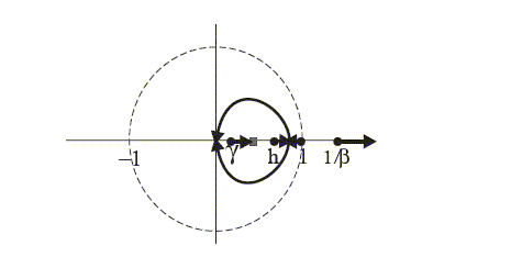
This diagram explains the position of the zeros as depicted in Figure 11 for low and high $\frac {\lambda }{\mu }$ . Finally if $\gamma>\frac{\mu h}{\phi+\mu}$ , it is easy to show that the root locus diagram changes very little. $\gamma$ will still have an arm connecting it to $\frac{\mu h}{\phi+\mu}$ , but the arrow will point in the opposite direction.

C. Calibration

So far we have we have derived conditions for unique and stable equilibria with IFB rules in our two-bloc model in parametric form. To carry out the numerical procedure to calculate thresholds $\theta^S(j)$ and $\theta^D(j)$ , $j \ge2$ we need to calibrate the model's structural parameters. This allows us to investigate various issues. Assuming that one of the blocs in the model is the US and the other bloc is the euro area, for example, we can explore the implications of our analysis for monetary policy in these two blocs for plausible parameterization of the model. Finally, we can derive indeterminacy regions for combinations of parameters in the rules and so identify parameter choices that shield from indeterminacy. Given these regions, we can also examine whether current policies in the US and the euro area are sufficiently insulated from the risk of indeterminacy. And in case they are not, we can draw policy implications and indicate whether and how policies can be made more robust to the possibility of sunspot sequences. Accordingly, we set our baseline calibrated values in line with prior empirical estimates on US and euro area quarterly data.

Table 2 below describes these parameters and explains where they come from. Most of the calibration is based on Smets and Wouters (2002, 2003. SW02 and SW03 henceforth) Bayesian estimates on US and area-wide data, respectively, of a one-country dynamic stochastic general equilibrium model. SW's model is similar to Christiano et al. (2001), CEE). SW's model differs from our two-bloc model inasmuch as: (i) in addition to nominal rigidities in both the price level and its growth rate, it assumes rigidities also in the wage level and its growth rate. In practice, SW02 and SW03 find that, for both the US and the euro area, rigidities in wages tend to be neither important nor significant. So SW03 provide alternative estimates of the structural parameters in their model obtained when they relax the wage stickiness assumption. It is these estimates to which we calibrate our model, given that we assume throughout that wages are flexible;(ii) it assumes capital accumulation with capital adjustment costs, whereas we assume that capital is constant in our model; (iii) finally, SW's model assumes a Cobb-Douglas technology for firms, whereas we, as Clarida et al (2002), assume that technology is of the CES form. Given these model differences, we cannot infer all parameters we need from SW02, SW03 estimates, so we calibrate the remaining parameters as in CEE and Erceg et al (2000, EHL) for the US bloc.

Table 2: Calibrated Values

Parameter	Notation	US Value	US Source	EA Value	EA Source
Discount factor	$\beta$	0.99	SW03,EHL	0.99	SW02
Risk Aversion	$\sigma$	2.01	SW03	1.61	SW02
Disutility of Effort	$\phi$	0.83	SW03	0.76	SW03
Indexation	$\gamma$	0.48	SW03	0.41	SW02
Calvo Probability	$\xi$	0.5-0.9	EHL, SW03	0.91	SW02
Habit	h	0.49-0.63-0.7	SW03,CEE	0.54	SW02

References

Aoki, M. (1981). Dynamic Analysis of Open Economies. Academic Press.

Batini, N. and Haldane, A. G. (1999).Forward-looking rules for monetary policy. In J. B. Taylor, editor, Monetary Policy Rules, pages 157-202. Chicago: University of Chicago Press.

Batini, N. and Nelson, E. (2001). Optimal horizons for Inflation Targeting. Journal of Economic Dynamics and Control, 25, 891-910.

Batini, N. and Pearlman, J. (2002). Too Much Too Soon: Instability and Indeterminacy With Forward-Looking Rules. Bank of England External MPC Discussion Paper No. 8.

Batini, N., Harrison, R., and Millard, S. (2003). Monetary Policy Rules for Open Economies. Journal of Economic Dynamics and Control, forthcoming.

Benhabib, J., Schmitt-Grohe, S., and Uribe, M. (2001). Monetary Policy and Multiple Equilibria. American Economic Review, 91(1), 167-86.

Benigno, G. and Benigno, P. (2001). Implementing Monetary Cooperation through Inflation Targeting. New York University, Mimeo.

Bernanke, B. and Woodford, M. (1997). Inflation Forecasts and Monetary Policy. Journal of Money Credit and Banking, 24, 653-684.

Black, R., Cassino, V., Aaron, D., Hansen, E., Hunt, B., Rose, D., and Scott, A. (1997). The Forecasting and policy System: The Core Model. Research Paper No. 43, Reserve Bank of New Zealand, Wellington.

Blanchard, O. J. and Kahn, C. M. (1980). The Solution of Linear Difference Models under Rational Expectations. Econometrica, 48(5), 1305-11.

Bullard, J. and Mitra, K. (2001). Learning about monetary policy rules. Journal of Monetary Economics.

Carlstrom, C. T. and Fuerst, T. S. (1999). Real indeterminacy in monetary models with nominal interest rate distortions. Federal Reserve Bank of Cleveland working paper.

Carlstrom, C. T. and Fuerst, T. S. (2000). Forward-looking versus backward-looking Taylor rules. Federal Reserve Bank of Cleveland working paper.

Castelnuovo, E. (2003). Taylor Rules and Interest Rate Smoothing in the US and EMU. mimeo, Bocconi University.

Chari, V. V., Christiano, L. J., and Eichenbaum, M. (1998). Expectation traps and discretion. Journal of Economic Theory, 81(2), 462-92.

Christiano, L. J., Eichenbaum, M., and Evans, C. (2001). Nominal Rigidities and the Dynamic Effects of a Shock to Monetary Policy. NBER Working Paper, no. 8403.

Clarida, R., Galí, J., and Gertler, M. (1999). The Science of Monetary Policy: A New Keynesian Perspective. Journal of Economic Literature, 37(4), 1661-1707.

Clarida, R., Galí, J., and Gertler, M. (2000). Monetary Policy Rules and Macroeconomic Stability: Evidence and Some Theory. Quarterly Journal of Economics, 115(1), 147-80.

Clarida, R., Galí, J., and Gertler, M. (2002). A Simple Framework for International Monetary Policy Analysis. NBER Working Paper w8870 .

Coletti, D., Hunt, B., Rose, D., and Tetlow, R. (1996). Bank of Canada's New Quarterly Projection Model. Part 3, The Dynamic Model: QPM. Technical Report No. 75, Bank of Canada, Ottawa.

Corsetti, G., Dedola, L., and Leduc, S. (2002). Consumption and Real Exchange Rates with Goods and Asset Markets Frictions. University of Rome III, Mimeo.

Currie, D. and Levine, P. (1993). Rules, Reputation and Macroeconomic Policy Coordination. CUP.

De Fiore, F. and Liu, Z. (2002). Openness and Equilibrium Determinancy under Interest Rate Rules. European Central Bank, WP. no. 173.

Devereux, M. B. and Yetman, J. (2002). Menu costs and the long-run output-inflation trade-off. Economic Letters, 76(1), 95-100.

Erceg, C. J., Henderson, D., and Levin, A. T. (2000). Optimal monetary policy with staggered wage and price contracts. Journal of Monetary Economics, 46(2), 281-313.

Evans, G. W. and Honkapoja, S. (2001). Expectations and the stability problem for optimal monetary policies. working paper, www.valt.helsinki.fi/RAKA/seppo.html.

Evans, G. W. and Honkapoja, S. (2002). Monetary policy, expectations and commitment. mimeo.

Evans, W. R. (1954). Control Systems Dynamics. McGraw Hill.

Faust, J., Rogers, J., and Wright, J. (2001). An Empirical Comparison of Bundesbank and ECB Monetary Policy Rules. International Finance Discussion Papers No. 705, Board of Governors of the Federal Reserve System.

Giannoni, M. and Woodford, M. (2002). Optimal Interest-Rate Rules: I. General Theory. NBER Working Paper no. 9419.

Karanassou, M., Sala, H., and Snower, D. (2003). A Reappraisal of the Inflation-Unemployment Trade-off. IZA Discussion paper No. 636, Bonn.

Kerr, W. and King, R. G. (1996). Limits on interest rates rules in the IS model. Economic Quarterly, 82(2), 47-76.

Levin, A., Wieland, V., and C, W. J. (2001). The performance of inflation forecast-based rules under model uncertainty. Federal Reserve Board International Finance Discussion Paper No.

McCallum, B. T. (1995). Two fallacies concerning central bank independence. American Economic Review, AEA papers and proceedings.

Sargent, T. and Wallace, N. (1975). Rational expectations, the optimal monetary instrument and the optimal money supply rule. Journal of Political Economy, 83, 241-54.

Smets, F. and Wouters, R. (2002). An estimated stochastic dynamic general equilibrium model of the Euro Area. European Central Bank, WP. no. 171.

Smets, F. and Wouters, R. (2003). Shocks and frictions in US business cycles: a Bayesian DSGE approach. paper presented at the conference `Dynamic Models Useful for Policy' held at the Bank of Canada, July 2003.

Sutherland (2002). International monetary policy coordination and financial market integration. mimeo, Board of Governors of the Federal Reserve System.

Svensson, L. E. O. (2001). Requiem for Forecast-Based Instrument Rules. mimeo, Stockholm University.

Svensson, L. E. O. (2003). What is wrong with Taylor Rules? Using judgement in monetary policy through targeting rules. Journal of Economic Literature, forthcoming.

Svensson, L. E. O. and Woodford, M. (1999). Implementing Optimal Policy through Inflation-Forecast Targeting. mimeo, Princeton University.

Svensson, L. E. O. and Woodford, M. (2003). Implementing Optimal Policy through Inflation-Forecast Targeting. mimeo, Princeton University.

Taylor, J. B. (1993). Discretion versus policy rules in practice. Carnegie-Rochester Conference Series on Public Policy, 39, 195-214.

Taylor, J. B. (1999). A Historical Analysis of Monetary Policy Rules. In J. B. Taylor, editor, Monetary Policy Rules, pages 319-41. Chicago: University of Chicago Press.

Tetlow, R. J. (2000). The Fed is Not as Ignorant as You Think. mimeo, Board of Governors of the Federal Reserve System.

Tetlow, R. J. and von zur Muehlen, P. (2001). Simplicity vesus optimality: The choice of monetary policy rules when agents must learn. Journal of Economic Dynamics and Control, 25, 245-79.

Woodford, M. (1999). Commentary: How Should Monetary Policy Be Conducted in an Era of Price Stability? In F. R. B. of Kansas City, editor, New Challenges for Monetary Policy. Kansas City: Federal Reserve Bank of Kansas City.

Woodford, M. (2000). Pitfalls of forward-looking monetary policy. American Economic Review, 90(2), 100-104.

Woodford, M. (2003). Foundations of a Theory of Monetary Policy. Princeton University Press.

Footnotes

* The paper is partly based on research conducted while Levine and Pearlman were visiting the European Central Bank (ECB) July-August 2003 as part of their Research Visitors Programme. Thanks are owing to the ECB for this hospitality and to numerous resident and visiting researchers for stimulating discussions. Views expressed in this paper do not reï¿½ect those of the BoE or the ECB. This paper was presented at the International Research Forum on Monetary Policy in Washington, DC, November 14-15, 2003. Insightful comments from discussants Giancarlo Cosetti and Marc Giannoni, and from other participants are acknowledged. Useful comments from an anonymous referee and from participants at seminars in Pompeu Fabra, the University of Frankfurt, the ECB, the Bank of England, the Bank of Canada and the Swiss National Bank are also gratefully acknowledged. Return to text

† Research Adviser, MPC Unit, Bank of England, Threadneedle Street, London EC2R 8AH, United Kingdom. E-mail: nicoletta.batini@bankofengland.co.uk. Return to text

‡ Professor of Economics, University of Surrey, Guildford, Surrey GU2 7XH, United Kingdom. Email: p.levine@surrey.ac.uk. Return to text

§ Professor of Economics, London Metropolitan University, 31 Jewry St, London EC3N 2EY, United Kingdom. Email: pearlman@lgu.ac.uk. Return to text

1. However, as we discuss in the next section, it has been argued that results such as these may be susceptible to the Lucas Critique. Return to text

2. Both types of real indeterminacy can be illustrated in a very simple closed economy model: consider a special case of `Phillips Curve' set out in this paper, $\pi _{t}=\mathcal{ E}_{t}(\pi _{t+1})+ay_{t}$ , where $\pi _{t}$ denotes inflation and $y_{t}$ is the deviation of output from its equilibrium level. Close the model with an ad hoc `IS' curve $y_{t}=-b(i_{t}-\mathcal{E}_{t}(\pi _{t+1}))$ where $i_{t}$ is the nominal interest rate which is set according to an IFB-Taylor rule $i_{t}=\theta \mathcal{E}_{t}(\pi _{t+1})+\mu y_{t}$ . Substituting out for $y_{t}$ and $i_{t}$ we arrive at $\mathcal{E}_{t}(\pi _{t+1})=\frac{ 1+b\mu }{1+b\mu -ab(\theta -1)}\pi _{t}$ which has a unique rational expectations solution $\pi _{t}=0$ iff $\frac{1+b\mu }{1+b\mu -ab(\theta -1)} >1$ and a stable trajectory, tending to zero inflation in the long run, consistent with any initial inflation rate otherwise- that is there is indeterminacy if $\theta <1$ or $\theta >1+\frac{2(1+b\mu )}{ab}$ . In the latter case, overly aggressive feedback produces cycles of positive and negative inflation. Thus the inclusion of a feedback on output reduces the region of indeterminacy. Empirical estimates of $\mu$ appear to be small, as discussed in section 2. So, in our subsequent analysis, we focus exclusively on `pure' IFB rules, i.e. rules without an output gap term. Return to text

3. Perhaps the closest paper to ours is De Fiore and Liu (2002) which explores indeterminacy in a small open-economy model with one-quarter-ahead IFB rules. Return to text

4. Giannoni and Woodford (2002) obtain similar results for IFB rules, but without interest rate smoothing. Return to text

5. The fact that forward-looking behavior is a source of indeterminacy can again be illustrated using the simple model of the previous footnote. Consider a rule involving a feedback on current inflation and the current output gap: $i_{t}=\theta \pi _{t}+\mu y_{t}$ . Then re-working the analysis we arrive at $E_{t}(\pi _{t+1})=\frac{1+b\mu +a\theta (1+(b+1)\mu )}{1+b\mu +a(1+(b+1)\mu )}$ which has a unique RE solution $\pi _{t}$ iff $\theta >1$ . For this current-looking rule there is no upper-bound on $\theta$ : all values above 1 ensure determinacy. Return to text

6. As we shall see in section 5, this a property of the optimal commitment rule. Return to text

7. Although empirical evidence seems to lend support to the idea that the US and European central banks follow IFB-type rules, the Lucas Critique suggests that there is a logical distinction between observing that a simple reduced-form relationship holds between variables and assuming that such a relation holds as a structural equation. For example, Tetlow (2000) demonstrates that a Taylor rule may seem to explain US monetary policy even if monetary policy is set optimally, conditioning on literally hundreds of state variables. Return to text

8. De Fiore and Liu (2002) assume this latter type of cash-in-advance assumption. Return to text

9. Batini et al. (2003), however, present a small open-economy model with a timing assumption on transactions as in Carlstrom and Fuerst (1999). De Fiore and Liu (2002) show that indeterminacy results are sensitive to the various assumptions on the timing of transactions in the context of a small open-economy model. Return to text

10. The population in each bloc is normalized at unity. It is straightforward to allow for different sized blocs, as in CGG (2002) and BB. Then in the Aoki decomposition, aggregates must be population-weighted and differences expressed in per capita terms. Return to text

11. Any welfare analysis and the formulation of optimal rules of the IFB form would require a stochastic treatment that now characterizes much of the New Keynesian literature. Return to text

12. When $h\neq 0$ , $\sigma$ is merely an index of the curvature of the utility function. Return to text

13. The effect of home bias in open economies is studied in Corsetti et al. (2002) and De Fiore and Liu (2002). Return to text

14. Thus we can interpret $\frac{1}{1-\xi }$ as the average duration for which prices are left unchanged. Return to text

15. In a stochastic setting with complete asset markets, (23) is simply the risk-sharing condition for consumption, because it equates marginal rate of substitution to relative price, as would be obtained if utility were being jointly maximized by a social planner (see Sutherland (2002)). Return to text

16. In effect, this is the case studied by De Fiore and Liu (2002) in a small open-economy context. Return to text

17. That is, for a typical variable $X_{t}$ , $x_{t}=\frac{X_{t}-\bar{X}}{\bar{X}}\simeq \log \left( \frac{X_{t}}{\bar{X}}\right)$ where $\bar{X}$ is the baseline steady state. Return to text

18. Our linearized system is in agreement with that of Christiano et al. (2001), BB and CGG(2002). Return to text

19. If , this replicates the result in CGG (2002). Return to text

20. Empirical work by Karanassou et al. (2003) gives a inflation rate -unemployment rate slope of around 3. Using calibrated values given in Appendix C, our model also suggests a significant long-run trade-off, but a rather smaller one than that estimated by these authors. Return to text

21. The correspondence is not exact as the quadratic approximation is about a carefully chosen cooperative flexible price steady state in which a subsidy rate is used to correct the distortion caused by imperfect competition. Moreover the inflation rates are for producer price and not consumer inflation as in (43). In an earlier paper Clarida et al. (1999) provide a strong defence of the pragmatic approach which is also adopted by Svensson (2001, 2003). Return to text

22. In a stochastic version of the model, if we assume simple AR(1) stochastic processes for the TFP shocks, i.e., $a_t=\varrho a_{t-1}+\epsilon_t$ , $a_t^*=\varrho^* a_{t-1}^*+\epsilon_t^*$ , then a term $\mathsf{F}\left[ \epsilon_t, {\epsilon_t^*} \right]^T$ where $\epsilon_t$ and $\epsilon_t^*$ are white noise disturbances would be added to the right-hand-side of (44). Return to text

23. Alternatively the policymaker might penalize changes in the interest rate. If neither penalty applies (i.e., $\alpha_i=0$ ), then the optimization problem must be set up as a two-stage procedure in which inflation rates are chosen optimally and then interest rates are set to achieve the resulting optimal paths for inflation. Return to text

24. See Svensson and Woodford (2003). An alternative form of the rule is as a specific targeting rule which takes the form of the first-order conditions that lead up to (45). Return to text

25. Non-certainty equivalence also has the consequence that optimal simple rules designed at time for displacements $z_{0}$ will be sub-optimal at any later date t where $z_{t}\neq z_{0}$ ; i.e., optimal simple rules are time inconsistent, even in the absence of forward-looking behaviour in the model. This, in essence, is the main point made in Svensson (2001). Return to text

26. These issues concerning the design of simple rules are addressed extensively in Currie and Levine (1993). Return to text

27. For instance (46) can be written as $\Delta i_{t}=\frac{1-\rho }{\rho }[\theta \mathcal{E} _{t}\pi _{t+j}-i_{t}]$ which is a partial adjustment to a static IFB rule $i_{t}=\theta \mathcal{E}_{t}\pi _{t+j}$ . Return to text

28. For the case of , we can substitute out for $\mathcal{E}_{t}(\pi _{H(t+1)})$ and $\mathcal{E}_{t}(\pi _{F(t+1)})$ from (44). Return to text

29. In this plane, the horizontal axis depicts real numbers, and the vertical axis depicts imaginary numbers. If a root is complex, i.e. , then its complex conjugate is also a root. Thus the root locus is symmetric about the real axis. Return to text

30. How we find the position of these zeros is main example of Appendix B. Return to text

31. Thus Figure 3 portrays diagrammatically the result shown analytically by Woodford (2003), chapter 4, that there is a value of $\theta =\theta ^{S}$ say, beyond which there is indeterminacy. Return to text

32. Results using MATLAB are reported in the next section. Return to text

33. An alternative way of handling the foreign assets problem is to follow BB and CGG, among others, and recast the model as stochastic with complete asset markets. Then, as mentioned in footnote 10, the relationship between foreign and domestic consumption and the real exchange rate derived in our perfect foresight model from the Euler equations and the UIP condition is still valid, but now becomes a risk-sharing condition. The linearized stochastic model has an identical deterministic component and therefore the stability analysis, which is all that concerns us in this paper, all goes through as before. Furthermore, in that case the analysis is valid without restrictions and $\sigma$ for the home bias case. Although now trade balance is not zero, the current account is balanced with any trade imbalance automatically offset by payoffs from income-contingent assets (see Sutherland (2002)). Return to text

34. Note that the decoupled interest rate process has a characteristic equation $z-\rho -\theta (1-\rho )z^{j}=0$ . By the root locus method it can be shown that this system also has an indeterminate equilibrium for and for when $\theta >\frac{1-\rho }{1+\rho }$ . However, for the system as a whole the indeterminacy is determined by that of the $y^{D},\pi ^{D}$ system as given in the proof. Return to text

35. In fact it is straightforward to show that proposition 4 also holds for any backward lag, . Return to text

36. As measured respectively by changes in the Harmonized Index of Consumer Prices, HICP; and changes in the Personal Consumption Expenditure, PCE, in the form of either the chain-weighted index or the deflator. Return to text

37. See Devereux and Yetman (2002) for a recent paper with endogenous Calvo price adjustments. Return to text

38. This range could include rules which also feedback on output and on future average inflation over a given time horizon j, rather than one-period inflation j periods ahead as in this paper. Return to text

This version is optimized for use by screen readers. A printable pdf version is available.

Indeterminacy with Inflation-Forecast-Based Rules in a Two-Bloc Model*

NON-TECHNICAL SUMMARY

Figure 1: Possible position of zeroes when

Figure 2: Position of zeroes as changes using current inflation

Figure 3: Position of zeroes as changes: 1-period ahead expected inflation

Figure 4: Position of zeroes as changes: 2-period ahead expected inflation

Figure 5: Position of zeroes as changes: 3-period ahead expected inflation

Figure 6: Position of zeroes as changes: 4-period ahead expected inflation

Figure 7: Position of zeros as changes: 3-period ahead expected inflation, and low

Figure 8: Areas of Determinacy for the Sum Difference Systems: Feedback on Producer Price Inflation and No Home Bias.

Figure 9: Position of zeroes as changes, for in the home bias difference system with CPI inflation based IFB rules.

Figure 10: Position of zeroes as changes, for in the home bias difference system with CPI inflation based IFB rules.

Figure 11: Position of zeros for varying

Table 2: Calibrated Values

Footnotes

Indeterminacy with Inflation-Forecast-Based Rules in a Two-Bloc Model^*

Figure 1: Possible position of zeroes when $\theta =0$

Figure 2: Position of zeroes as $\theta$ changes using current inflation

Figure 3: Position of zeroes as $\theta$ changes: 1-period ahead expected inflation

Figure 4: Position of zeroes as $\theta$ changes: 2-period ahead expected inflation

Figure 5: Position of zeroes as $\theta$ changes: 3-period ahead expected inflation

Figure 6: Position of zeroes as $\theta$ changes: 4-period ahead expected inflation

Figure 7: Position of zeros as $\theta$ changes: 3-period ahead expected inflation, and low $\rho$

Figure 9: Position of zeroes as $\theta$ changes, for in the home bias difference system with CPI inflation based IFB rules.

Figure 10: Position of zeroes as $\theta$ changes, for in the home bias difference system with CPI inflation based IFB rules.

Figure 11: Position of zeros for varying $\frac {\lambda }{\mu }$