Skip to: [Printable Version (PDF)]

Board of Governors of the Federal Reserve System
International Finance Discussion Papers
Number 841, September 2005 --- Screen Reader Version*

House Prices and Monetary Policy: A Cross-Country Study

Alan G. Ahearne, John Ammer, Brian M. Doyle, Linda S. Kole, and Robert F. Martin^*

NOTE: International Finance Discussion Papers are preliminary materials circulated to stimulate discussion and critical comment. References in publications to International Finance Discussion Papers (other than an acknowledgment that the writer has had access to unpublished material) should be cleared with the author or authors. Recent IFDPs are available on the Web at http://www.federalreserve.gov/pubs/ifdp/. This paper can be downloaded without charge from the Social Science Research Network electronic library at http://www.ssrn.com/.

Abstract:

This paper examines periods of pronounced rises and falls of real house prices since 1970 in eighteen major industrial countries, with particular focus on the lessons for monetary policy. We find that real house prices are pro-cyclical--co-moving with real GDP, consumption, investment, CPI inflation, budget and current account balances, and output gaps. House price booms are typically preceded by a period of easing monetary policy, but then diminishing slack and rising inflation lead monetary authorities to begin tightening policy before house prices peak. In a careful reading of official reports, speeches, and minutes, we find little evidence that foreign central banks have reacted to past episodes of rising real house prices beyond taking into account their implications for inflation and output growth. However, central bankers have expressed a range of opinions in the more recent policy debate with some willing in certain cases to raise policy rates to try to stem current and future surges in asset prices while others favor moral suasion or a hands-off approach. Finally, we characterize the risks associated with house-price reversals. Although mortgage lenders in some countries have significant exposure to house prices, the balance of evidence suggests that this exposure does not, in and of itself, pose a significant risk to financial stability. Nevertheless, the co-movement of both property prices and default rates with the business cycle means that losses on mortgage lending are likely to be higher when banks' other lines of business are also performing poorly.

Keywords: Asset prices, business cycles, bubbles, financial stability

JEL classification: E44, E52, E58, F41

1  Introduction

House prices have risen markedly in recent years in many industrial countries amid low long-term real interest rates, ample liquidity, and steady economic growth. Not only have prices risen rapidly in real terms, but also they have increased relative to income and rents, and there are signs that speculative activity has picked up in some markets. Industrial economies have experienced significant rises and falls in real house prices on a number of occasions over the past thirty-five years. If the current episodes follow the typical pattern seen in the past, real house prices may eventually slow in a number of countries, and some countries could endure a period of flat or even falling real prices in the future.

Like other asset prices, house prices are influenced by interest rates, and in some countries, the housing market is a key channel of monetary policy transmission. Indeed, house prices appear to be associated with business-cycle movements in a number of real variables, such as consumption and investment. Nevertheless, there is no consensus as to whether accommodative policy has contributed to "excess" volatility in house or other asset prices, either recently or in previous episodes. Because house prices, monetary variables and macroeconomic aggregates also move in response to other shocks hitting the economy, the direction or extent of causality between these variables can be difficult to disentangle. For instance, after the stock market decline and economic downturns around 2000-2001, monetary policy eased in many industrial countries, and that may have helped foster financial conditions favorable for the latest run-up in house prices and also may have forestalled more serious downturns in economic activity. Although monetary policy has become less accommodative in a number of countries recently, global long-term interest rates have remained low and house prices have continued to climb.

Goals for asset prices--including house prices--are not among the specific mandated objectives of central banks, but clearly house price swings can have important implications for economic activity and inflation. The consequences of sharp movements in house prices for financial stability also need to be taken into account by central banks and by supervisory agencies that regulate financial institutions. In the past, major declines in real house prices have often been associated with economic downturns, and have at times contributed to financial distress, particularly when nominal collateral values also declined significantly.

Recently, the word "bubble" has been increasingly used in press and market commentary on house price developments. This paper does not take a stand on whether or not any particular real estate market is currently experiencing a bubble. Even if we agreed on the best model of house price determination, bubbles are intrinsically hard to define and to identify--especially while they are occurring--because it is very difficult to differentiate between price changes coming from underlying economic fundamentals (some of which are unknown, unobservable, or unquantifiable) and those based on "irrational exuberance." Moreover, most economic research to date has had limited empirical success in explaining, much less predicting, asset prices.

This paper examines periods of pronounced rises and falls of real house prices in eighteen major industrial countries and attempts to draw lessons for monetary policy.¹ We have divided it into six sections. After this brief introductory summary, we present some facts on the evolution of real house prices from 1970 to the present. In section 3, we analyze past episodes of real house price appreciation and depreciation, characterize their common features, and describe the behavior of other key macroeconomic variables during these episodes. We find that real house prices are pro-cyclical and tend to reach a maximum near business cycle peaks, often after a prolonged period of buoyant growth in activity has raised output above its potential level and inflation pressures have begun to emerge. Subsequently, real house prices fall for about five years, on average, and their previous run-up is largely reversed. Real GDP growth slows during the first year or so after house prices peak, as do growth rates of private consumption and investment.

House price booms are typically preceded by a period of easing monetary policy, with policy rates bottoming out about the same time that house prices take off, about three years before house prices peak. Policy rates remain low for a little more than a year but then rise steadily through the years before and after the house-price peak, during which CPI inflation continues to rise. Rates then reverse quickly in response to falling GDP growth, widening output gaps, and lower inflation. Broad money growth is generally higher before the peak than afterward.

Co-movement with other long-term asset prices is also a feature of house price cycles. In past episodes, real long-term interest rates tended to be at a low about two years before real house prices peaked, increased as the peak approached, and continued to rise for several quarters after the peak before gradually trending down. Real equity prices tended to peak four to eight quarters before real house prices.

In the fourth section of the paper, we consider monetary policy reactions to house price swings. We have found little evidence in central bank reports, speeches, and minutes that foreign central banks have reacted to past episodes of rising real house prices beyond taking into account their implications for inflation and output growth. Of course, because house prices have tended to move with output gaps and inflation, we find it challenging--even after the fact--to infer empirically which variables were driving policy. Looking at policy statements made during a number of episodes, we find that central bankers have emphasized variables such as inflation and exchange rates rather than movements in asset prices. However, the question of what central banks should do remains open, with some subset of foreign central bankers apparently willing to raise policy rates to try to stem current and future surges in asset prices and another group preferring only to use moral suasion or to take a hands-off approach. The recent discussions by officials of the Bank of England and the Reserve Bank of Australia are instructive examples of this debate.

In section 5, we assess the risks associated with potential reversals in house prices. Property owners are most directly vulnerable to the risk of a house price decline (especially if they lose their jobs in an economic downturn), and in some countries, mortgage lenders also have significant exposure to nominal house prices. Although securitization of residential mortgages has grown rapidly abroad, it is far less developed in most countries than in the United States, so most mortgage lending largely remains on the books of the lender. However, the financial system stress experienced by a number of countries in the 1990s was more directly linked to declines in the value of commercial property collateral rather than residential property, with the exception of the United Kingdom. Financial institutions are able to carry substantial exposure to residential mortgages for several reasons: Residential property prices are relatively stable, loans are not typically made for the full value of the property, and loan-to-value ratios fall over the life of the loan. All these factors contribute to low default rates on mortgages and high recovery rates on foreclosures. Moreover, most foreign lenders with exposure to mortgage debt appear to be well capitalized so that their equity holders are likely to bear most of this risk.

We also document that U.S. investors have very limited exposure to movements in foreign real estate prices. In contrast, the residential construction sectors abroad are much more vulnerable to corrections in local house prices. We present the results of simple simulations for several countries to give an idea of the expected magnitude of such an adjustment for their construction sectors. We close with some tentative conclusions.

2  Features of House Prices in Industrial Economies

2.1  Behavior of House Prices since 1970

Real house prices in the foreign industrialized economies have exhibited prolonged rises and falls over the past thirty-five years (see chart 2.1).² In almost all eighteen countries for which we have data, real house prices are characterized by episodes of long rises followed by protracted falls, and most of the countries have experienced rapidly rising house prices for the past several years. In the Netherlands, Australia, and the United Kingdom, house price increases seem to have begun to moderate. In Japan, real house prices have been declining since 1991. German real house prices have also been gradually declining since they reached a modest peak in 1994, which coincided with a construction boom.

Several of the real house price series seem to trend upward, at least since the mid-1980s. We might expect to see a positive trend in real house prices in countries with growing populations. Land, an important factor in housing, is in fixed supply. Population growth increases the density of the housing stock, and this effect is exacerbated by the trend toward urbanization in many of these countries. As density increases, housing becomes relatively scarce, and its relative price rises. Another factor underlying the trend may be different productivity performance across sectors. For example, if productivity gains are greater in the consumer-goods sector than in the construction sector, then consumer goods will become less costly to produce, and the relative price of housing will increase.

The vertical lines in chart 2.1 indicate "peak" dates for real house prices in each country. Across all the countries, we identify forty-four peaks, twenty-six of which occurred before 1985. For this exercise, we define a peak as a centered six-year high in real house prices excluding end points. That is, at the peak, the level of real house prices is higher than at any point three years on either side of the peak. Our definition prevents us from identifying any peaks occurring after 2001.³ For each country, we identify at least one peak between 1970 and 2004, and in some cases, we find as many as four.⁴ On average, real house prices rise around 28 percent over the five years preceding a peak and fall about 22 percent in the five years after a peak.

The blue shading in chart 2.1 indicates peak-to-trough recession dates as chosen by the National Bureau of Economic Research for the United States and the Economic Cycle Research Institute for other countries (where available). For many of these countries, the dating of business cycles indicates that a recession typically occurred soon after the peak in real house prices. Below we show that real house prices tend to be pro-cyclical. Peaks in commercial property prices (not shown) also coincide with many of the peak dates in house prices, especially in the late 1980s and early 1990s. In contrast, several countries appear to have experienced a peak in commercial property prices around 2000, a date preceding the recent acceleration in house prices.

Changes in house prices seem to be positively correlated across countries, suggesting that global factors (such as low real interest rates or global business cycles) are important determinants of house price cycles.⁵ Chart 2.2 shows a time series for the number of countries experiencing four-quarter declines in real house prices (the dashed red line) and the number of countries experiencing four-quarter increases of real house prices that are more than twice their average pace of increase (the solid black line). By this metric, there have been four major episodes of relatively fast house price increases--1973-74, 1978-79, 1986-89, and recently. Each of the past episodes of rapid price increases was followed by a period in which a large number of countries experienced real house price declines. The number of countries that experience real house price declines is generally larger than the number of countries that experienced high growth in the preceding period. The difference is not surprising given our asymmetric definition of increases and decreases, but it does imply that a country does not necessarily have to incur exceptionally rapid growth to be at risk for a real decline. In addition, the fact that neither line reaches zero in any period implies that during the peak years some countries are still experiencing house price declines and during the bust years a few countries are experiencing faster than normal growth. Therefore, while global factors may be important, idiosyncratic shocks to individual countries are also playing a role. Finally, note that the current peak stands out in the sense that a historically high number of countries in our sample recently experienced abnormally rapid rises in house prices. If these prices follow the same patterns as before, house prices in a large number of these countries are likely to decline in real terms at some point in the not-too-distant future.

2.2  Measures of Valuation

Chart 2.3 shows ratios of nominal house prices to disposable income for eight countries.⁶ Using this measure to determine the valuation of housing is complicated by the fact that the ratio seems to trend in a number of countries. Although the ratio appears to be mean-reverting in the United Kingdom, Australia and the Netherlands, it seems to have trended down in the United States, Germany, Japan, Sweden and Australia, at least until 2001. In contrast, the ratio has trended up in Spain. Large deviations from trend tend to coincide with sharp movements in house prices, and these deviations eventually seem to be reversed. All the countries shown, with the exception of Germany and Japan, have ratios of house prices to disposable income that are above what would have been predicted based on their trends; however, recent movements of the U.K. and Australian ratios stand out. In both of these countries, these ratios are near record highs. The increase in these ratios (relative to trend) raises concerns over the sustainability of house prices, particularly in the United Kingdom and Australia.

Another commonly used measure of house price valuation is the ratio of house prices to rents. This ratio serves as an indicator of house valuation in much the same way that the price-to-earnings ratio serves for equity evaluation. Chart 2.4 shows price-to-rent ratios for the countries for which we have the longest time series. Price-to-rent ratios are at highs in the United Kingdom, Australia, and the United States. In contrast, in Japan, where the housing market has been in decline for almost fifteen years, the ratio seems to be approaching a record low.

Because asset prices are forward looking and thus embody expectations of future changes in the economic environment, it is difficult to judge, using these indicators alone, whether prices are out of line with their equilibrium values. Nevertheless, past experience tells us that, when these indicators deviate significantly from trend, they tend to move back toward historical norms. In a recent FEDS paper, Joshua Gallin (2004) shows that the U.S. price-to-rent ratio tends to move back toward its historical trend, with prices tending to adjust faster than rents. If the series for other counties exhibit similar properties, then countries with above-trend price-to-rent or price-to-income ratios are likely to undergo future periods in which house prices increase more slowly than rents or incomes or perhaps even fall in real terms.

2.3  Evidence of Speculation in Housing

The rise in house prices coupled with the rise in the traditional valuation ratios described above raises concerns about the sustainability of house prices. Some commentators argue that unreasonable expectations of future capital gains are driving house prices. If overly optimistic expectations are a significant driver of house price changes, one might expect a surge in purchases of housing as a pure investment vehicle.⁷ If these expectations prove wrong, investment properties are more likely to return to the market than are owner-occupied houses, increasing the supply of housing and perhaps accelerating a decline in prices.⁸

Data on investment properties are not available for most countries. However, the data we do have indicate that in some countries these types of purchases have increased over the past several years. Chart 2.5 shows the volume of "buy-to-let" lending as a percentage of total mortgage lending in the United Kingdom and lending to investors as a percentage of total mortgage lending in Australia. Data for the United Kingdom are semi-annual and go back only to 1999. Since then, buy-to-let lending has increased from about 3 percent of total mortgage lending to around 7 percent. The decline in this ratio in the second half of 2004 coincides with slowing appreciation of U.K. house prices. For Australia, a longer time series is available on a monthly basis. Lending to investors increased from around 15 percent of total mortgage lending in 1992 to nearly 40 percent at the end of 2003, surpassing its previous high around the time of the 1989 house price peak; but it has since declined to around 34 percent with the sharp slowdown in house prices. However, we doubt that all the variation can be attributed to speculative activity because much of the increase predated the period of rapidly rising house prices. In addition, the recent increase was nowhere near as dramatic as the sharp one that occurred in 1989.

3  House Prices, Financial Conditions, and Real Economic Activity

To explore the interaction of house prices with other elements of the financial and economic environment, we studied the behavior of key financial and macroeconomic indicators around the times of peaks in house prices. We calculated the median value of these indicators around all the forty-four peaks in our sample.⁹ Our results are presented in the form of "event graphs," in which the quarter of the peak is designated quarter 0, so that quarter 8, for example, refers to the eighth quarter after the peak in house prices was reached.

To briefly preview our results, we find that house prices are highly pro-cyclical, with swings in house prices associated with both swings in economic performance and changes in monetary policy.¹⁰ Based on our findings, we cannot rule out the possibility that monetary policy may have contributed to house price booms and busts and resulting fluctuations in real economic activity. However, the close association between real house prices and the other economic and financial indicators may largely reflect the endogenous response of house prices to shocks in aggregate economic activity, with monetary policy responding to these shocks and to the expected path for inflation.

Nominal policy interest rate: As shown in chart 3.1, the early phase of the run-up in real house prices is associated with declines in nominal policy interest rates. Around six to eight quarters before the peak, rates begin to move up. Several quarters after house prices have peaked, policy rates turn down, falling more than 4 percentage points over the next twelve quarters or so.

Inflation: Headline CPI inflation, shown in chart 3.2, begins to pick up a few quarters before the house price peak and continues to move higher even after house prices have turned down, topping out around quarter 4. Inflation then eases noticeably, ending up several percentage points below its initial value by quarter 20.

Real GDP growth: Real GDP growth, shown in chart 3.3, is robust during most of the upswing in house prices, registering a median of around 4 percent during much of the pre-peak period. Median growth begins to drop markedly in the quarter preceding the peak and bottoms out at a small negative rate about five quarters after the crest in house prices. Growth then starts to trend up, returning to near its pre-peak pace by quarter 20.

Output gap: As shown in chart 3.4, real GDP tends to grow faster than potential GDP during house price booms, with the level of actual output about 2 percent above the level of potential output in quarter 0. House price booms seem to coincide with overheating in real economic activity. The reversal in house prices is associated with the slowing of output to below the pace of potential output, with an output gap of nearly (negative) 2 percent by quarter 16.

Real personal consumption growth: The pattern of personal consumption around peaks (chart 3.5) is similar to the pattern of real GDP growth described above.

Real total investment growth: Run-ups in house prices are associated with a heady pace of total investment growth (chart 3.6), though investment appears to begin to cool around four quarters before house prices peak. Investment plunges in the quarters immediately following the peak and continues to contract up to quarter 12. For a limited number of peaks for which data on disaggregated investment spending are available, the evidence suggests that the boom and bust are more pronounced in residential investment than in other types of investment spending.

Real long-term interest rate: The real rate was calculated as the nominal long-term interest rate minus an estimate of long-term inflation expectations.¹¹ In theory, lower real interest rates should raise house prices. As shown in chart 3.7, long-term rates initially decline until around ten quarters before the peak in house prices. Rates then remain relatively low until quarter -4, at which stage they begin to move up. Interestingly, long-term real rates appear to remain relatively elevated after the peak, trending down only slowly, even as policy rates and house prices are falling.

Money supply growth: As shown in chart 3.8, growth in M3, although volatile, appears considerably lower on average in the period after the peak in house prices than in the period before the peak. This result is not surprising because growth in M3 is positively correlated with growth in real GDP and household borrowing.

Real stock prices: As shown in chart 3.9, stock prices and house prices tend to move up together, though the gains in house prices outstrip those in stock prices. Compared with house prices, stock prices appear to turn down earlier and experience a steeper decline. After quarter 8, stock prices rebound, even as house prices continue to decline.

Budget balance: As shown in chart 3.10, the fiscal deficit narrows over much of the period preceding the peak in house prices, though some deterioration appears to begin in quarter -4. The fiscal deficit widens significantly in the aftermath of the downturn in house prices, reaching nearly (negative) 5 percent of GDP about four years after the peak. These patterns are consistent with cyclical movements in budget balances resulting from fluctuations in economic activity that often accompany house price booms and busts.

Current account: The current account deficit, shown in chart 3.11, begins to widen noticeably at least eight quarters before the crest in house prices, reaching about 2½ percent of GDP in quarter 0. The deficit widens a bit more immediately following the peak and then begins to shrink gradually as house prices decline, with the current account balance close to zero by the time real house prices stabilize around quarter 20. The adjustment in the current account reflects the slump in investment and the rise in household saving rates during the economic downturn following the peak in house prices.

3.1  Pre-1985 and Post-1985 Subsamples

Our full sample extends back to 1970 and so covers the high inflation period of the 1970s and early 1980s as well as the relatively low inflation period since about 1985. As we note below, many countries deregulated their mortgage markets during the early to mid-1980s. As a check on the robustness of our findings across these very different periods, we examine the behavior of indicators around house price peaks in the pre-1985 period and in the period from 1985 onward (post-1985) separately. For most indicators, the results for the pre-1985 and post1985 samples are broadly similar. Perhaps not surprisingly, the largest differences between our two subsamples are in the behavior of median inflation and nominal policy interest rates. Whether these differences reflect changes in the behavior of inflation and policy rates around house price peaks or around business cycle peaks is not clear, however, given the close association between real house prices and economic performance.

Inflation: The behavior of median CPI inflation across our two subsamples, shown as the solid red lines in chart 3.12, appears noticeably different. During house price booms in the pre1985 period, inflation at first declined from very high rates and then increased a year or so before the house price peak. In the post-1985 period, in contrast, inflation appears to trend sideways during the house price run-up. In both the pre-1985 and the post-1985 samples, the downturn in house prices is associated with declines in inflation that begin one or two years after the house price peak.

Nominal policy interest rates: In both the pre-1985 and post-1985 samples, the early stages of house price booms take place against a backdrop of reductions in policy interest rates. Policy rates then begin to move up. The hikes in the policy rate come later and are much larger in the pre-1985 case, as central banks react to the sharp upturn in inflation, than in the post-1985 case. In the aftermath of the peaks, when house prices are falling, central banks appear to have cut policy rates more quickly and sharply in the post-1985 era than in the earlier period.

3.2  Demographics

Demographic factors appear to have played a role in the differing patterns of house price movements across countries. As shown in chart 3.13, growth rates in the working-age population have picked up since the early 1990s in several countries that have experienced large run-ups in house prices in recent years, including Australia, Ireland, the United Kingdom, and the United States. For example, Ireland's annual population growth averaged about 1¾ percent over the past decade and boosted the demand for houses. In Australia, Canada, Ireland, New Zealand and the United States, high rates of immigration have helped drive population growth. In contrast, the declines in house prices in Japan and Germany over the past decade were concurrent with dramatic slowdowns in population growth, with populations actually declining in recent years.

In addition, demographic changes in industrial countries may be affecting house prices through the effect of population aging on saving rates and interest rates. As large cohorts of baby boomers prepare for retirement in many countries, saving rates should rise, pushing down long-term real interest rates and boosting house prices.

3.3  Other Factors: Financial Deregulation, Innovation, and Structural Changes

Financial deregulation has often been pointed to as a possible culprit for the large run-up in house prices experienced by many countries in the late 1980s.¹² Indeed, a look at table 3.1 shows that in the 1980s a large portion of the countries in our sample experienced some sort of mortgage market deregulation. By the end of the 1980s, most constraints in most industrial countries had been lifted. Much of the deregulation eased constraints on household borrowing. In the United Kingdom, the United States, France, Canada, and Denmark, the deregulation increased the pool of potential lenders by lifting constraints on eligible lenders. In Australia, Denmark, Finland, Japan, Sweden, and the United States, removing the regulations pertaining to the interest rates paid by borrowers and the interest rates paid to lenders increased the willingness and ability of borrowers and lenders to arrange mortgages. These changes may also have boosted competition in the lending market as financial institutions sought to establish or protect market share.

In principle, if more households can finance the purchase of a house and the supply of housing is limited, house prices should rise. We do not find any evidence inconsistent with the notion that financial deregulation contributed to run-ups in house prices except to note that two earlier global house price episodes--in 1973 and 1979--occurred before any significant deregulation.

Structural changes in markets or in the level of government intervention in markets may also have affected the level of house prices. For example, homeowners' interest deductibility from taxes in the United Kingdom was progressively decreased during the 1990s and finally eliminated in 2000; some commentators have suggested that this change may have contributed to the fall in U.K. house prices in the first half of the 1990s. The Australian government appears to have contributed to an acceleration of house prices around 2001, when it offered a grant for first-time home buyers and lowered the effective rate of capital gains tax on rental properties.

Structural changes may also make prices more sensitive to other shocks. For example, land use restrictions have become increasingly common over time. While these restrictions may have only small contemporaneous effects, they may reduce the long-run supply elasticity and make house prices more sensitive to future shocks.¹³ Again, the overall effect of these structural changes is difficult to measure, but it may be significant.

The changes in the 1990s are probably not as sweeping as those that occurred in the 1980s, but they have been significant. Some of the recent innovations appear in table 3.2. Most of the mortgage innovations listed in the chart, taking the form of extended terms and greater

availability of variable rate loans, offer households greater choices.¹⁴ The increased availability of online mortgages and refinance facilities also may have lowered access costs.

3.4  The Current Episode

What light, if any, can the patterns documented above shed on the current episode of rapidly rising house prices? Given the relationships observed in the historical data, does the recent behavior of financial and macroeconomic indicators suggest that real house prices are currently near a peak? To try to answer these questions, we consider a hypothetical exercise in which we assume that house prices peaked in each country in the fourth quarter of 2004.¹⁵ Charts 3.14 through 3.21 plot the median values for a range of indicators over the twenty quarters from the fourth quarter of 1999 to the fourth quarter of 2004.

One point to note in passing is that (median) real house prices moved down a bit during the global economic downturn in 2001. However, because the decline in the level of house prices did not last at least three years, we do not identify 2001 as a house price peak. The mildness of the dip in house prices probably reflects the shallow nature of the economic downturn. Indeed, despite the slowing of growth, for many countries we do not identify an actual recession, and for the remaining countries the recession was mild by historical standards. In addition, the rise in policy interest rates (shown in chart 3.14) that preceded the 2001 dip in house prices was moderate compared with the increases seen around previous house price peaks (see chart 3.1).

If a house price peak occurred in the fourth quarter of 2004, how did the behavior of our indicators around that date compare with the patterns observed around previous peaks? Comparing the movements in median policy interest rates in chart 3.1 and chart 3.14, what is striking is that we have not seen recently the sizable increases in policy rates that typically precede house price peaks. If the fourth quarter of 2004 was a house price peak, the absence of a pronounced hike in median policy interest rates in 2003 and 2004 would make it a highly unusual peak. Of course, policy rates have increased in several countries, including Australia, the United Kingdom, and the United States, so the patterns in these countries would match somewhat better with previous peaks. Moreover, the median output gap (shown in chart 3.17) was close to zero in late 2004, with no evidence of the overheating in economic activity usually associated with run-ups in house prices. As such, the recent booms in residential investment in many countries have helped support economic growth and reduce slack in these economies.

Equally striking is that, after falling in 2002, real long-term interest rates (chart 3.20) stayed low in 2003 and 2004 (and have declined even more since), an observation that again is not typical in the quarters preceding a house price peak (see chart 3.7). Moreover, long-term rates have remained low even in countries where central banks have been hiking policy rates.

4  Monetary Policy Reaction to House Price Swings

We have little empirical evidence to show that foreign central banks changed their policy rates beyond what would be necessary to react to the implications of house prices for inflation and output growth. Both median policy rates across all housing market episodes (chart 3.1) and policy rates in some particular episodes (chart 4.1) reach their peak near the peak in house prices. As we have already pointed out, swings in house prices tend to be pro-cyclical--output gaps (chart 3.4) and inflation (chart 3.2) also tend to peak around the median house price peak. Empirically it would be difficult to tell whether monetary policy was reacting to house prices as well as output gaps and inflation. For instance, given how difficult measuring output gaps is and given the strong co-movement in house prices and output gaps, comparing actual policy rates to the policy rates implied by a standard Taylor rule would not necessarily tell us whether central banks were reacting to house prices. For example, if a standard Taylor rule fitted policy rates well, it house prices might still have been an important factor driving policy behavior. Moreover, if a standard Taylor rule failed to predict policy rates well, it need not do so because house prices are important. Monetary policy may be reacting to other variables, such as oil shocks, productivity shocks, or exchange rates, or more subtly, house prices may be correlated with the measurement error in output gaps.

In the rest of this section we explore central banks' own descriptions of their actions, which may be a better indicator of the importance of house prices in the formulation of monetary policy. We focus on six important episodes--in Japan, Sweden, the United Kingdom, and Australia in the late 1980s and early 1990s (chart 4.1) and in Australia and the United Kingdom in recent years (chart 4.2)--as well as some recent speeches by central bankers from other foreign countries. The early episodes suggest that central banks in these countries focused primarily on inflation and exchange rates and paid relatively little attention to residential or commercial property prices. The recent speeches suggest that the debate about how central banks should react to house and other asset price swings is still an open one, with some foreign central bankers willing to shift the stance of monetary policy if it would restrain substantial and abnormally rapid rises in asset prices.

4.1  Past Episodes

During many of the episodes of house price swings before 1985, particularly around 1973 and 1979, central banks appeared to be focused more directly on inflation, on the effects of oil shocks, and on exchange rates than on house prices. Likewise, during the house price swings of the late 1980s and early 1990s in Japan, Sweden, Australia, and the United Kingdom, explanations of monetary policy emphasized exchange rates and inflation as the most important monetary policy objectives. In the mid-to-late 1980s, in Japan and the United Kingdom, the central banks lowered interest rates primarily to limit exchange rate appreciations and, in Australia's case, to prevent an appreciation that would further widen the current account deficit. In Sweden and in the United Kingdom after October 1990, monetary policy was used to maintain exchange rate pegs. Outside these periods, the central banks focused on inflation--tightening monetary policy to prevent inflation from rising around the time of house price peaks and lowering rates by less to allow inflation to come down afterward. In part, the exchange rate pegs adopted in 1990 were to provide a nominal anchor to help lower inflation.¹⁶

In most of these countries, monetary policy was eased in the years before house price peaks, tightened in the run-up to the peak and beyond it, and then eased in subsequent years (consistent with the behavior of median policy rates around house prices outlined in the previous section), but there is little evidence that monetary policy was altered in response to house prices. House prices did not figure prominently in the rationales given for monetary policy during the tightening phases. Indeed, in Britain, at the peak of the house price boom in third quarter of 1989, the housing market was not specifically identified as a risk to the inflation outlook.¹⁷ Japan was an exception in that the rapid growth in monetary aggregates and asset prices concerned the Bank of Japan (BOJ), but inflation was low from 1986 to 1988, and "[p]olicymakers felt that, for their actions to gain public support, they would need absolutely solid evidence of inflationary potential building up" (Yamaguchi, 1999).

Some of these central banks may have failed to give sufficient consideration to the effect of property prices on output growth and inflation. The Bank of England (BOE) later said that it had made policy mistakes and forecasting errors associated with financial developments during this period and should have raised interest rates earlier (Leigh-Pemberton, 1990). The Reserve Bank of Australia (RBA), like the BOE, later stated that it had been slow to realize that demand was rising quickly and that it had not fully appreciated the impact of financial developments on output and inflation.¹⁸

Finally, some BOJ officials have expressed skepticism about the ability of earlier tightening to stem the rise in asset prices or of more aggressive easing of policy to mitigate Japan's subsequent malaise, and they have noted that easing too early might have re-ignited the "bubble" (Yamaguchi, 1999 and 2002).

4.2  Recent Debate

Central bankers in Britain, Australia, and other industrial economies have recently debated how central banks should react to substantial rises in asset prices in the wake of the sharp decline of equity prices in 2000 and the steep rise in house prices over the past several years. In their more recent speeches, all these policymakers generally shun extreme positions, such as ignoring asset price movements or targeting a particular value of any asset. They indicate, in particular, that monetary policy should not be aggressively tightened in an attempt to "prick" an asset price "bubble." Beyond this agreement on the extremes, these central bankers have not come to a firm consensus on the appropriate reaction. Some would argue that central banks should react to asset prices only to the extent that they contain information about output growth and inflation. Others would argue that central banks should "lean against" sustained and abnormally rapid increases in asset prices.

Nowhere has the debate been more public than in the United Kingdom, where house prices have almost tripled over the past nine years, with the largest gains occurring from late 2001 through the first half of 2004 (chart 4.2, upper panels). Starting in November 2003, the Monetary Policy Committee (MPC) of the Bank of England gradually raised the repo rate 125 basis points, to 4.75 percent. In its minutes and in most members' speeches that address those rate increases, the MPC states that it looks at house prices (and asset prices more generally) only to the extent that they provide information relevant to future output growth and inflation.¹⁹

Without necessarily ascribing these views to most MPC members, the MPC statements are consistent with the view that central banks have no better information than market participants do regarding underlying asset price valuations. Although most foreign central bankers would caution that identifying an unsustainable rise in asset prices is very difficult, some of these policymakers would contend that doing so is virtually impossible. Furthermore, the appropriate monetary policy during a "bubble" is uncertain because the dynamics of a true bubble are uncertain and the lags of monetary policy are long. Monetary policy makers would not know whether to raise interest rates to deflate the bubble or to start lowering them to cushion the economy once the bubble bursts. Rather than explicitly targeting house or other asset prices, central banks can try to react to the inflation and output effects of sizable asset price movements and try to minimize threats to financial stability.²⁰

In Britain's case, the MPC arguably did more than just incorporate house prices into its forecasts. In an effort to smooth adjustment, the MPC publicly emphasized well in advance of its November 2003 tightening its intention to raise rates gradually, in part by highlighting that its inflation and GDP forecasts were based on an upward sloping path for interest rates. Furthermore, a number of MPC members have attempted to inform the public of the possibility of a slowdown in house price increases and have been talking about the consequences of households taking on large amounts of debt. Talking about such actions publicly might alter agents' behavior. However, those doing such "jawboning" might be perceived as having some notion of what the "correct" value of house prices is. Although not many central bankers, either at the BOE or elsewhere, have spoken about jawboning as a strategy that central banks might follow, a number of central bankers have warned households not to take on too much debt.

Even if a central bank reacts to house prices only to the extent that they affect inflation, how much it reacts depends on the way house prices are included in the inflation measure being targeted. As table 4.1 shows, price indexes in the foreign economies vary both in their inclusion of owner-occupier's imputed rents, a measure of the cost of consuming housing services, and in their method used to calculate imputed rents. The United States, for example, calculates imputed rents using a sample of rents on similar houses, whereas other countries, such as Australia, Canada, New Zealand, and Sweden, calculate imputed rents using some measure of house prices.

In December 2003, the British government changed the MPC's targeted inflation series from a series that includes imputed rents, the RPIX, to a series that does not, the CPI, and also adjusted its inflation target from 2½ percent to 2 percent.²¹ Imputed rents in the RPIX are calculated using a house price index. At the time of the switch, the MPC said that policy would be unaffected by the change in the target series, despite the exclusion of house prices, because it expected house price growth to abate in the medium run.

Some members of the MPC disagreed with the majority view and pushed for a steeper tightening of monetary policy over the course of the second half of 2003 and the first half of 2004.²² This minority has argued that, by increasing interest rates more than would be justified by the short-run effects of changes in house prices on output and inflation, the Committee might lower the probability of house prices rising further and households taking on more debt and, hence, might also lower the probability of the eventual consequences of this build-up.²³ Inflation would be further from its target than it would otherwise be in the near term but would be closer in the medium run. Financial stability could also be improved.

Other central bankers, including some at the Sveriges Riksbank, the Norges Bank, the Bank of Canada, and the Reserve Bank of New Zealand, have also argued that central banks should on rare occasions "lean against" exceptionally large surges in equity and property prices.²⁴ Some of these officials feel that restricting themselves to "cleaning up the mess" after real asset prices decline is an asymmetric response that encourages excessive asset price swings. Also, tightening more as asset prices rise would diminish market perceptions that there would be no consequences to investors' actions (Wadhwani, 2003).

Some central bankers argue that, although central banks should not target asset prices, they should look at the effects of the prices on inflation and output beyond the central bank's usual policy horizon.²⁵ In Australia, where annual house prices increased at a double-digit pace during the past several years, the RBA has raised its cash rate 125 basis points, starting in May 2002 (chart 4.2, lower panels). Although RBA Governor Ian Macfarlane (2004) said that house prices "are not appropriate targets for monetary policy" and Deputy Governor Glenn Stevens noted that central bankers should look at asset prices only for the information that they give us about the evolution of the macroeconomy, Stevens (2004) further cautioned that policy makers should not be confined to looking at their effects only at a one- or two-year horizon. The distinction between this position and "leaning against the wind" is quite subtle: In practice, monetary policy might look similar even though the rationale for it would be slightly different.

The recent experience in Britain suggests that communicating a particular monetary policy strategy to the public and to markets may be difficult during a substantial run-up in asset prices. Policymakers may easily be construed as trying to prick a bubble when they are only reacting to the effects of asset prices on output growth and inflation, jawboning, or leaning against the wind. As noted above, although there is some disagreement among MPC members, the majority view is that the MPC should not target assets prices, and those members have tried to articulate that view in the minutes and in their speeches. The until recently surging house prices coupled with the increased frequency of MPC members' comments on house prices may have fueled the perception by some that the Bank of England is targeting house prices. As MPC member Kate Barker noted in a recent speech (Barker, 2005), "Why do I feel reluctant to talk about housing? Quite simply, I don't want to add credence to the view that the outlook for house prices dominates our decisions..."²⁶

Some central bankers have emphasized that financial supervisors have an important role to play in monitoring banks' exposure to potential losses in the event of a slide in prices. As Issing (2003) points out, "... comparing the toolboxes of regulators and monetary policy authorities (in a narrow sense), it is clear that the former have an absolute advantage in caring for system wide stability of financial institutions, as they are able to define, monitor and enforce the rules of the game." Where the central bank is neither a bank regulator nor a supervisor, such as in Britain and Australia, some policymakers have warned of the need for vigilance in this regard.²⁷ In Australia, in particular, there is concern that the recent extension of credit to some borrowers who were unable to receive loans in the past may pose some risk to financial stability.²⁸

5  House Prices and Mortgage Finance: Who Bears the Risk?

In this section, we attempt to assess the risks associated with potential reversals in house prices. In particular, we try to shed some light on the exposure to house price downturns of different sectors of the economy--specifically homeowners, mortgage lenders, U.S. investors, and the construction industry.

5.1  Households

Not surprisingly, property owners appear to be the first and the most affected by fluctuations in house prices. For all the countries listed in table 5.1, except Germany, a majority of homes are owner-occupied, so that the household sector clearly bears much of the brunt of exposure to movements in house prices. Even for Germany, where the homeownership rate is only 42 percent, Casper (2004) estimates that 80 percent of Germany's 5 trillion euros of residential real estate is owned directly by the household sector, including a majority of rental properties.²⁹ To the extent that variable rate mortgages are more common outside the United States, households abroad have relatively more exposure to interest rate changes.

5.2  Mortgage lenders

Mortgage lenders can also be significantly exposed, although their risk is more closely tied to nominal house prices than to real house prices. The rightmost column of table 5.1 shows that mortgage lending varies in importance across countries. The lowest figure is for Italy, where there are legal impediments to enforceable liens against homeowners, with the foreclosure process reported to last for five to seven years. Not surprisingly, real estate lending in Italy is also characterized by both the most rapid amortization and the lowest initial loan-to-value (LTV) ratios of the countries listed in the table. Nevertheless, Italians still have the highest homeownership rate.

Somewhat in contrast to U.S. practice, mortgage lending is a significant activity for a number of large foreign banks. Table 5.2 lists several dozen depository institutions with more than $50 billion in real estate loans outstanding. In some cases, such property lending accounts for a substantial proportion of the bank's assets, and in most cases it easily exceeds both the stock market capitalization and the accounting net worth of the bank.³⁰ Nevertheless, the conventional market view is that most of these banks have ample capital to withstand the risks they are likely to face. Such a benign view is reflected in the last column of the table in Moody's bank financial strength ratings (BFSR), which assess the underlying creditworthiness of a bank in the absence of external support, such as public guarantees on bank liabilities, whether explicit or implicit. For a majority of the banks listed, the BFSR is in the B- to B+ range, indicating "strong intrinsic financial strength."

How is it that this substantial exposure to mortgage loans, which often can absorb much of a borrower's cash flow, is not judged to have more dire implications for the risk borne by lenders? A number of factors help limit the prospects of credit losses on mortgage loans. One factor is that some mortgage lenders have substantially reduced exposure by securitizing a significant portion of the loans that they originate. (We provide more detail on the extent of mortgage-related securitization outside the United States below.) Another factor is that nominal house prices are less volatile than commercial property prices.

Furthermore, loans are not typically made for the full value of the property. In addition, the LTV ratio typically falls as the loan ages, with collateral value usually rising (at least in nominal terms) and the loan balance amortizing. For example, a recent Moody's credit opinion for HBOS plc, the largest U.K. mortgage lender, reports an average LTV for the bank's mortgage portfolio of only 41 percent, with only 7 percent of the book at an LTV exceeding 85 percent. In Canada, mortgage borrowing with an LTV above 75 percent requires the purchase of insurance from a government agency. Not surprisingly, historical recovery rates from mortgage foreclosures have compared favorably to recoveries from corporate defaults. Furthermore, for a variety of reasons, a household might choose to continue to make mortgage payments (rather than undertaking a "strategic default") when the value of the home has fallen below the loan balance. The conventional wisdom in the mortgage industry is that unemployment is the primary cause of defaults.

The notion that residential mortgage lending is a low-risk activity generally is supported by some of the recent historical experience with banking system stress associated with declines in property prices. In particular, Japan, Sweden, and Norway experienced significant financial system stress in the early 1990s, including (at least de facto) major bank insolvencies. Although declines in the value of commercial property collateral were a factor in these episodes, residential mortgage lending was not. In the United Kingdom around the same time, however, household mortgage lending was an important component of the challenges confronting depository institutions. For example, chart 5.1 shows that mortgage repossessions rose in 1991-93 to nearly ten times their typical level in the 1970s. However, the major banks and building societies withstood the test fairly well. Even at their peak, foreclosure rates remained below 1 percent per year and, with substantial recoveries from re-selling repossessed properties, actual credit losses incurred by the lenders were an even smaller fraction of their mortgage portfolios. U.K. mortgage lenders may be even less vulnerable today because a significant proportion of U.K. mortgage borrowers since 1998 have purchased private mortgage insurance.

One of the consequences of the relatively benign experience with residential mortgage risk is that, at least for loans within specified LTV constraints, capital requirements will be reduced for residential mortgage loans under Basel II. Some of the details have been left to national supervisors.

A few individual lending institutions may be somewhat more vulnerable to house prices. The banks shown in boldface in the main part of table 5.2 and all the banks in the lower part of the table had mortgage loans outstanding that were at least ten times either the market capitalization or book equity of the bank. Interestingly, when the BFSR is available for a U.K. or Swiss lender among this group, it is always in the B range for this table, implying that the bank is amply capitalized, notwithstanding the highly leveraged exposure to mortgage lending. However, several of the German and Japanese banks in the table have a BFSR in the D or E category ("modest" or "very modest" intrinsic financial strength), although for the Japanese banks, the weak credit assessment has much more to do with their business lending activities.

Table 5.3 shows aggregate national figures reflecting all the individual banks for which we found mortgage loan data. Given other evidence about the relatively low levels of risk involved in residential mortgage lending, the figures do not suggest that mortgage lending poses a significant threat to the banking systems of these countries. To the extent that banks are sharing in exposure to real estate prices, the risk is borne largely by bank equity holders rather than other bank stakeholders because in most cases a bank's equity capital is so unlikely to be exhausted by mortgage losses.

5.3  Securitization

As a result of a well-developed market for residential mortgage-backed securities (RMBS), originators of U.S. mortgage lending need not retain significant exposure to borrowers or to the underlying collateral, and in practice less than one-third of U.S. mortgages are kept on the books of depository institutions.³¹ However, securitization of mortgages occurs to a much lesser degree in other countries. The upper panels of chart 5.2 show that mortgage securitization volumes in Europe have grown rapidly from very low levels in the 1990s, but with negligible levels of activity in major countries such as France and Germany.³² Even in the United Kingdom, which accounted for more than half of European issuance in 2004, the risk transfer from RMBS issued there last year was equivalent to only 19 percent of gross lending secured on dwellings, with the balance of mortgage exposure remaining on the books of the lenders.³³

The lower panels of chart 5.2 reveal a similar state of affairs in Australia and Canada. The proportion of outstanding mortgages included in securitizations has grown steadily in Australia since the mid-1990s but still stands at only 19.8 percent. For the four major Canadian banks for which data could be obtained the equivalent aggregate figure is 17.5 percent.

5.4  U.S. Investors

The gradual trend toward financial globalization raises the possibility that U.S. investors may have some exposure to house prices abroad through relatively direct channels. For U.S. banks, the principal mechanism is lending abroad. The upper panel of chart 5.3 shows that real estate loans of foreign offices of U.S. banks account for only about 0.5 percent of total assets. For the ten largest banks, the figure is twice as high (1 percent last year), but it has fallen from more than double that much over the past decade.

The lower panel, which is drawn from the Treasury International Capital (TIC) survey of international portfolio security holdings, shows that other U.S. investors also appear to have limited exposure to foreign real estate.³⁴ Aggregate U.S. portfolio investment in the foreign construction and real estate industries amounted to only $41 billion at the end of 2003, a relatively trivial fraction of the more than $3 trillion in total foreign portfolio investment of U.S. investors. Foreign asset-backed securities (ABS) accounted for an additional $65 billion in U.S. holdings, but likely only a fraction of the underlying collateral is real estate-related.

5.5  Nonfinancial Business: The Residential Construction Sector

The exposure of the domestic nonfinancial business sector to house price shocks may be more difficult to characterize than that of homeowners, financial institutions, or foreign investors, but it may be too important to ignore completely. In Germany, for example, fluctuations in investment in structures reportedly have been an important component of business cycle volatility in recent years. The solid lines in chart 5.4 show the residential construction share of GDP for four countries for which long data series were available. Clearly, home building is disproportionately sensitive to cyclical variations. Real house prices (the dashed lines) seem to be positively associated with the construction share. For example, in the United Kingdom, the residential construction share of GDP peaked at over 5 percent in 1989, after several years of rapidly rising home values, but then plummeted about 2 percentage points by early 1991, when property prices reversed direction.

To help get a sense of the magnitude of fluctuations in construction activity that typically has been associated with a given movement in property prices, for each of these countries we estimate a four-lag vector autoregression (VAR) model in (1) the quarterly change in the log of real house prices and (2) the construction share of GDP. The results are expressed in chart 5.5 as impulse responses to one-time 5 percent negative price shocks, with the dashed green line representing the path of real house prices and the solid black line the residential construction share of GDP.³⁵ Real house prices continue downward in subsequent quarters, leveling off after a total decline ranging from 8 percent in Canada to 17 percent in the United Kingdom. The estimated impact on construction activity is largest in Australia, with a peak effect approaching 0.4 percent of quarterly GDP. The estimated cumulative effect on the construction share tops out for Australia at 1.8 percent of quarterly GDP after seven quarters, compared with peak cumulative estimated effects of 2.5 percent for Canada, 0.7 percent for the United Kingdom, and just 0.2 percent for the Netherlands.³⁶

6  Conclusions

Foreign industrial economies have experienced many large swings in house prices over the past thirty-five years, and the latest rise has been the most dramatic on record. The extent of the rise and its synchronization across countries raises concerns that, if history is any guide, real house prices are quite likely to fall or at least stagnate in a number of industrial countries in the future. Furthermore, the pro-cyclicality of real house prices also suggests that their downward correction will be associated with some slowing of consumption and residential investment, which could contribute to an economic downturn.

Certain financial conditions (low interest rates, ample liquidity, and financial deregulation) were usually present in past house price surges and could conceivably raise the probability of their occurrence or the intensity of the rise, but other factors (business-cycle shocks, demographics) also helped explain these booms. Looking across episodes (including the most recent ones), monetary policy tended to be relatively easy as house prices began to accelerate (policy rates were low and broad money growth was rapid), but house prices continued to rise as central banks tightened in response to emerging inflation pressures and buoyant growth. Rapidly rising house prices seem to have coincided with overheating domestic demand and at times may have indicated that a turning point was imminent. Correlation is not the same as causation, however, so further empirical research is clearly needed.

Given the difficulties associated with identifying asset price bubbles, it is perhaps not surprising that central banks have not come to a firm consensus on how they should react to house or other asset prices that seem to have become unhinged from economic fundamentals. Some argue that central banks should "lean against" bubbles to avoid macroeconomic and financial instability. Others argue that central bankers should not try to second guess markets and instead should remain steadfast in their pursuit of low inflation or output stability objectives or both; they should be concerned about house price swings only insofar as they affect these objectives and financial stability.

In a few previous episodes, significant declines in nominal asset prices were associated with a rise in nonperforming loans and weakened bank balance sheets. However, residential mortgages generally have been low risk, and even though some lending institutions have substantial exposures, it is unlikely that residential mortgage lending poses a significant threat to banking systems in these countries. Households and residential construction companies also are exposed to the risk of interest rate increases and house price corrections, and they may be less prepared for an economic downturn. In those countries where the run-up in house prices appears to be most advanced--the Netherlands, Australia, and the United Kingdom--these risks seem to have been manageable thus far, but the adjustment process is still unfolding.

References

Ahearne, Alan, Joseph Gagnon, Jane Haltmaier, Steve Kamin, Christopher Erceg, Jon Faust, Luca Guerrieri, Carter Hemphill, Linda Kole, Jennifer Roush, John Rogers, Nathan Sheets, and Jonathan Wright (2002), "Preventing Deflation: Lessons from Japan's Experience in the 1990s," International Finance Discussion Paper 729, Board of Governors of the Federal Reserve System.

Aoki, Kosuke, James Proudman and Gertjan Vlieghe (2001), "Why Housing Prices Matter?" Bank of England, Quarterly Bulletin, Winter.

Ball, Michael (2005), "RICS European Housing Review 2005," Royal Institute of Chartered Surveyors report.

Bank of England (various), "Operation of Monetary Policy," Quarterly Bulletin, issues from February 1987 to November 1990.

Bank of England (1989), "General Assessment," Quarterly Bulletin, August.

Barker, Kate (2005), "The Housing Market and the Wider Economy," speech to the Institute of Economic Affairs, January 24.

Bean, Charles (2004), "Asset Prices, Monetary Policy, and Financial Stability: A Central Banker's View," speech to the American Economics Association, January.

Bell, Marian (2005), "Communicating Monetary Policy in Practice," Vital Topics Lecture at the Manchester Business School, May 17.

Bernanke, Ben, and Mark Gertler (2001), "Should Central Banks Respond to Movements in Asset Prices?" American Economic Review, 91(2), 253-57.

Bollard, Alan (2004), "Asset Prices and Monetary Policy," speech to the Canterbury Employers' Chamber of Commerce, January 30.

Bucks, Brian and Karen Pence (2005), "Measuring Housing Wealth," Board of Governors of the Federal Reserve System, January.

Bundesbank (2002), "The Housing Market During the 1990s," Monthly Report 54(1), January, 31-35.

Canada Mortgage and Housing Corporation (2004), "Canadian Housing Observer."

Cargill, Thomas, Michael Hutchison, and Takatoshi Ito (1997), The Political Economy of Japanese Monetary Policy, Cambridge, Massachusetts: MIT Press.

Case, Karl E., John M. Quigley and Robert J. Schiller (2005), "Comparing Wealth Effects: The Stock Market versus the Housing Market," Advances in Macroeconomics, B.E. Journals in Macroeconomics, 5(1).

Casper, Sigried (2004), "Chancen zur Wohneigentumsbildung," University of Tuebingen memorandum, January 28.

Catao, Luis, Thomas Helbling and Marco Terrones (2003), "When Bubbles Burst," in Chapter 2, World Economic Outlook, International Monetary Fund, Spring.

Cecchetti, Stephen, Hans Genberg, and Sushi Wadhwani (2003), "Asset Prices in a Flexible Inflation Targeting Framework," in W. Hunter, G. Kaufmann, and M. Pomerleano (eds.), Asset Price Bubbles, Cambridge, Massachusetts: MIT Press.

Debelle, Guy (2004), "Macroeconomic Implications of Rising Household Debt," BIS Working Paper 153, June.

Edge, Rochelle (2000), "The Effect of Monetary Policy on Residential and Structures Investment Under Differential Project Planning and Completion Times," Finance and Economic Discussion Series, Federal Reserve Board, 2000-673.

European Central Bank (2005), "Asset Price Bubbles and Monetary Policy," ECB Monthly Bulletin, April.

Fraser, Bernie (1991), "Some Observations on the Role of the Bank," speech to the Annual General Meeting of the Committee for Economic Development of Australia, November 28, in Reserve Bank of Australia Bulletin, December.

Gallin, Joshua (2004), "The Long-Run Relationship between House Prices and Rents," Finance and Economics Discussion Series, 2004-50, September.

Girouard, Nathalie, and Sveinbjörn Blöndal (2001), "House Prices and Economic Activity," OECD Working Paper no. 279.

Gjedrem, Svein (2003), "Financial Stability, Asset Prices, and Monetary Policy," speech to the Center for Monetary Economics, Norwegian School of Management, June 3.

Glaeser, Edward, and Joseph Gyourko (2002), "Zoning's Steep Price," Regulation, Fall, 24-30.

Gruen, David, Michael Plumb, and Andrew Stone (2003), "How Should Monetary Policy Respond to Asset-Price Bubbles?" in Anthony Richards and Tim Robinson (eds.), Asset Prices and Monetary Policy, Reserve Bank of Australia, 260-80.

Gurkaynak, Refet (2005), "Econometric Tests of Asset Price Bubbles: Taking Stock," Finance and Economics Discussion Paper, 4, Federal Reserve Board, January.

Issing, Otmar (2003), "Monetary and Financial Stability: Is There a Trade-off?" comments at the Bank for International Settlements, March.

Johnston, R.A. (1989), "Doing It My Way: Some Reflections of a Retiring Governor," address to Australian Business Economists, July 14, in Reserve Bank of Australia Bulletin, August.

King, Mervyn (2004), Speech to the Confederation of British Industry Scotland Dinner, June 14.

Large, Andrew (2004), "Puzzles in Today's Economy--the Build up of Household Debt," speech to the Association of Corporate Treasurers' Annual Conference, March 23.

Leigh-Pemberton, Robert (1990), "Monetary Policy in the Second Half of the 1980s," Bank of England, Quarterly Bulletin, May.

Lindberg, Hans, and Christina Lindenius (1991), "The Swedish Krona Pegged to the Ecu," Sveriges Riksbank, Quarterly Review, Third Quarter.

Lomax, Rachel (2004), "Keeping the Party under Control--Anniversary Comments on Monetary Policy," speech to the Annual Luncheon of the British Hospitality Association, July 1.

Macfarlane, Ian (2004), "Monetary Policy and Financial Stability," speech to CEDA Annual Dinner, November 16.

Monetary Policy Committee (2004), "Minutes and Press Notices," Bank of England, August.

Ringström, Olle (1987), "The Exchange Rate Index: An Instrument for Monetary and Exchange Rate Policy," Sveriges Riksbank, Quarterly Review, Fourth Quarter.

OECD (2004), "Housing Markets, Wealth and the Business Cycle," OECD Economic Outlook, June.

Otrok, Christopher, and Marco E. Terrones (2005), "House Prices, Interest Rates, and Macroeconomic Fluctuations: International Evidence," a paper presented at the conference, Housing, Mortgage Finance, and the Macroeconomy, a conference hosted by the Federal Reserve Bank of Atlanta, May.

Phillips, M.J. (1988), "Flamingoes and Hedgehogs," address to the Australian Society of Corporate Treasurers, October 24, in Reserve Bank of Australia Bulletin, November.

Phillips, M.J. (1990), "Decisions: Decisions!" address to the Rotary Club of Sydney, August 14, in Reserve Bank of Australia Bulletin, September.

Scanton, Kathleen, and Christine Whitehead (2004), "International Trends in Housing Tenure and Mortgage Finance," Council of Mortgage Lenders Research, November.

Schiller, Robert J (2005), Irrational Exuberance, second edition, Princeton, New Jersey: Princeton University Press.

Selody, Jack, and Carolyn Wilkins (2004), "Asset Prices and Monetary Policy: A Canadian Perspective on the Issues," Bank of Canada Review, Autumn.

Srejber, Eva (2005), "The Role of Asset Prices and Credit in an Inflation Targeting Policy," remarks at the Swedish Royal Institute of Technology, March 16.

Stevens, G.R. (2004), "Recent Issues in the Conduct of Monetary Policy," speech to Australian Business Economists at the Economic Society of Australia on February 17, Reserve Bank of Australia Bulletin, March.

Sveriges Riksbank (1990), "Monetary and Foreign Exchange Policies in 1989," Quarterly Review, First Quarter.

Sveriges Riksbank (1991), "Monetary and Foreign Exchange Policies in 1990," Quarterly Review, First Quarter.

Terrones, Marco (2004), "The Global House Price Boom," in Chapter 2, World Economic Outlook, International Monetary Fund, Autumn.

Walley, Simon (2005), "Capital Adequacy and Property Valuation," presentation to the European Mortgage Federation, April 20.

Wellink, Nout (2002), "Central Banks as Guardians of Financial Stability," speech to the Central Bank of Aruba, De Nederlandsche Bank, November 14.

Yamaguchi, Yutaka (1999), "Asset Prices and Monetary Policy: Japan's Experience," in Proceedings of a Conference on New Challenges for Monetary Policy, Federal Reserve Bank of Kansas City, August 26-28.

Yamaguchi, Yutaka (2002), "Monetary Policy in a Changing Economic Environment," Economic Review, Federal Reserve Bank of Kansas City, Fourth Quarter.

Data Appendix

Real house and equity prices. We use data on real house prices and real equity prices provided by the Bank for International Settlements (BIS). The BIS collects the data from national sources (see table A1). The nominal house price series for France, Italy and Japan are semi-annual and the series for Germany is annual. The BIS interpolates these countries' series to the quarterly frequency using a cubic spline. Finally, the BIS deflate each of the house and equity price series by its respective country's private consumption deflator.

We define house price peaks as a centered six-year high in real house prices excluding end points. That is, at the peak, the level of real house prices is higher than at any point three years on either side of the peak. Our definition prevents us from identifying any peaks occurring after 2001. These house price peak dates are the following: Australia 1974Q1, 1981Q2, 1989Q2, 1994Q3; Belgium 1979Q3; Canada 1976Q4, 1981Q1, 1989Q1; Denmark 1973Q3, 1979Q2, 1986Q1; Finland 1974Q1, 1989Q2, 2000Q2; France 1981Q1, 1991Q1; Germany 1974Q1, 1982Q1, 1994Q2; Ireland 1979Q2, 1990Q3; Italy 1974Q4, 1981Q2, 1992Q2; Japan 1973Q4, 1990Q4; Netherlands 1978Q2; New Zealand 1974Q3, 1983Q1, 1996Q2; Norway 1976Q4, 1987Q2; Spain 1978Q2, 1991Q4; Sweden 1979Q3, 1990Q1; Switzerland 1973Q1, 1989Q4; United Kingdom 1973Q3, 1980Q3, 1989Q3; United States 1973Q4, 1979Q2, 1989Q4.

Business-cycle dates. We use U.S. business-cycle peak and trough dates from the National Bureau of Economic Research (NBER). For all other countries, where available, we use dates from the Economic Cycle Research Institute. These dates are the following: Australia June 1974 - January 1975, June 1982 - May 1983, June 1990 - December 1991; Canada April 1981 -November 1982, March 1990 - March 1992; France July 1974 - June 1975, August 1979 - June 1980, April 1982 - December 1984, February 1992 - August 1993; Germany August 1973 - July 1975, January 1980 - October 1982, January 1991 - April 1994, January 2001 - August 2003; Italy October 1970 - August 1971, April 1974 - April 1975, May 1980 - May 1983, February 1992 - October 1993; Japan November 1973 - February 1975, April 1992 - February 1994, March 1997 - July 1999, August 2000 - April 2003; New Zealand April 1974 - March 1975, March 1977 - March 1978, April 1982 - May 1983, November 1984 - March 1986, September 1986 - June 1991, October 1997 - May 1998; Spain March 1980 - May 1984, November 1991 - December 1993; Sweden October 1970 - November 1971, July 1975 - November 1977, February 1980 - June 1983, June 1990 - July 1993; Switzerland April 1974 - March 1976, September 1981 - November 1982, March 1990 - September 1993, December 1994 - September 1996, March 2001 - March 2003; United Kingdom September 1974 - August 1975, June 1979 - May 1981, May 1990 - March 1992; United States December 1969 - November 1970, November 1973 - March 1975, January 1980 - July 1980, July 1981 - November 1982, July 1990 - March 1991, March 2001 - November 2001.

Disposable income. We use quarterly data, where available, from the OECD outlook database. Data for Germany and Japan are only available annually.

Rental price data. For each country, we use the sub-index of the consumer price index for rental housing. Where available, we use actual rents rather than owner-occupied imputed rents. We do not adjust the rental data for potential biases.

Mortgage lending to investors. The percent of mortgage lending to investors as a percentage of total mortgage lending for Australia come from the Reserve Bank of Australia. The data on "buy-to-let" lending as percentage of total mortgage lending are from the Council of Mortgage Lenders in the United Kingdom.

GDP, consumption and investment. We use quarterly real GDP, consumption and investment data from the first quarter of 1970 until the final quarter of 2004. For each country, we use official national series as reported by Haver Analytics from the starting point of the relevant series to the end of the sample. In cases where the current vintage of national accounts data does not extend back to 1970, we splice data from official series of an older vintage. To splice the data, we use the quarterly growth rates from the earlier data along with the first level in the recent data to construct a new level series extending back to 1970Q1.

We handle German reunification by taking the quarterly growth rates of West German GDP, investment and consumption for the period up to and including the first quarter of 1991, the quarter of reunification; growth rate data are for united Germany thereafter. To create a level series consistent with the units for united Germany, we use the splicing method described above.

Output gaps. We use OECD estimates of the output gap from the OECD economic outlook database. The data are at a quarterly frequency from 1970 to 2004 (including forecast). Output gaps are expressed as the percentage that actual output is greater (positive gap) or less (negative gap) than its potential level.

Consumer price indexes. For each country we use the four-quarter change in the headline CPI series as reported by Haver Analytics from the starting point of the relevant series to the end of the sample. In cases where central banks have a targeted inflation series, we use that series. In cases where the current targeted series does not extend to 1970, we splice data of an older vintage official series. To splice the data, we use the splicing method above.

Current account and fiscal balance to GDP. We use quarterly data on the ratio of the current account balance to GDP from national sources as reported by Haver Analytics, where available. We splice earlier data, where available from the OECD economic outlook database and the IMF's International Financial Statistics. We use quarterly data on the ratio of the government fiscal balance to GDP ratio from the OECD economic outlook database, where available. All current account data start in 1970 (and end in 2004) with the exceptions of Denmark(for which the series starts in 1978), Finland, Ireland, and Sweden(1975), Germany and Italy(1971), and Switzerland(1972). All government balance data start in 1970 (and end in 2004) with the exceptions of Belgium(1970Q2), Denmark(1971Q2), Ireland(1977), Norway(1975Q2), New Zealand(1986Q2), and Switzerland(1990). No quarterly government balance data are available for Japan.

Policy rates. We use quarterly data on the nominal policy rates from national sources as reported by Haver Analytics, where available. We splice earlier data, where available from the OECD outlook database. Data available starting in 1970 with the exceptions of Australia (1979), France(1974), Norway(1977Q2), the Netherlands(1982), New Zealand(1985), Spain(1977Q3), Sweden(1974Q2), and Switzerland(1972).

Real long-term interest rates. We use quarterly average real 10-year benchmark yields from 1971 to 2004 for the following countries: Australia, Belgium, Canada, France, Germany, Italy, Japan, Spain, Sweden, Switzerland, the United Kingdom and the United States. The Netherlands is available only from 1973. Inflation expectations are derived based on data from surveys of professional economic analysts taken from Consensus Forecasts.

M3. For each country, we use the national series for M3 as reported by Haver Analytics from the starting point of the relevant series to the end of the sample. For the United States, we use M2. Data start in 1970 (and end in 2004) with the exceptions of Belgium (1996Q4), Denmark (1993), Finland (1990), France, Germany, and Japan (1980), Italy (1997), the Netherlands (1982Q4), New Zealand (1988), Norway (1992Q4), Spain (1997Q3), Sweden (1985), Switzerland (1985), and the United Kingdom (1982Q2).

Population. We use annual data from the OECD economic outlook database. We use working age population, age 15 to 64.

U.K. repossessions. We use U.K. properties taken into possession as reported by the Council of Mortgage Lenders in the United Kingdom.

Construction output. We use quarterly construction output as a share of GDP in the United Kingdom, Australia, Canada and the Netherlands from national sources.

Table 3.1:  Deregulation of the Mortgage Market

Country	Year	Deregulatory Action
Australia	1982	Quantitative lending guidance eliminated
Australia	1986	Removal of ceiling on mortgage interest rate
Canada	1967	Ceiling on interest rates on bank loans eliminated
Canada	1967	Restrictions on banks' participation in mortgage financing abolished
Canada	1980	Banks allowed to have mortgage loan subsidiaries
Denmark	1982	Liberalization of mortgage contract terms
Denmark	1982	Interest rate deregulation
Denmark	1989	Elimination of restrictions on mortgage bond issuance
Finland	1984	Funding quotas from the Central Bank to commercial banks eliminated
Finland	1986	Interest rate deregulation
Finland	1987	Guidelines on mortgage lending removed
France	1984	Bank specialization requirements reduced
France	1987	Elimination of credit controls
Germany	1967	Interest rate deregulation
Italy	1983	Interest rate deregulation
Italy	1983	Credit ceilings eliminated (temporarily reimposed 1986-87)
Japan	1993	Bank specialization requirements reduced
Japan	1994	Interest rate deregulation completed
Netherlands	1980	Interest rate deregulation
New Zealand	1984	Credit allocations guidelines removed
New Zealand	1984	Interest rate deregulation
Norway	1984	Lending controls abolished
Norway	1985	Interest rate deregulation
Sweden	1985	Interest rate deregulation
Sweden	1985	Lending controls for banks abolished
United Kingdom	1980	Credit controls (corset) eliminated
United Kingdom	1981	Banks allowed to compete with building societies for housing finance
United Kingdom	1986	Building societies allowed to expand lending activities
United Kingdom	1986	Guidelines on mortgage lending removed
United States	1980	Interest rate deregulation, phasing out of Regulation Q (deposit interest rate ceilings) over four years
United States	1980	Elimination of portfolio restrictions for thrifts

Source: Girouard and Blöndal (2001), table 3.

Table 3.2:  Recent Mortgage Product Innovations in Selected Countries

Country	Recent Innovations
Australia	Flexible mortgages with variable repayments
Australia	Home equity loans
Australia	Split-purpose loans (splits loan into two sub-accounts, giving tax advantages)
Australia	Deposit bonds (insurance company guarantees payment of deposit at settlement)
Australia	Non-conforming loans
Australia	Redraw facilities and offset accounts
Australia	New providers including mortgage originators and brokers
Belgium	Loans available up to 30 years
Canada	Shorter-term mortgages, initial fixed-rate period shortened from 5 years to 1 year
Canada	Skip-a-payment, early mortgage renewal, and flexible payment schedules
Denmark	"Interest-adjusted" loans, interest rate set at regular intervals by sale of bonds
Denmark	Capped-rate loans
Denmark	BoligXloans: Interest adjusted every six months with reference to 10 day average of CIBOR
Denmark	Interest-only loans
Finland	Lengthening mortgage terms
Finland	Introduction of state guarantee for mortgages
France	Variable-payment mortgages
Netherlands	Savings or equity mortgages: Part of payment covers interest, part goes into fixed-interest savings account or equity account (confers tax advantages)
Netherlands	Interest-only loans
United Kingdom	Flexible mortgages
United Kingdom	Offset mortgages (savings and mortgage held in same/linked accounts, with savings offset against mortgage balance)
United Kingdom	Base-rate trackers

Source: Scanton and Whitehead (2004) and Canada Mortgage and Housing Corporation (2004).

Table 4.1:  Housing Costs in Consumer Price Indices in Selected Industrial Countries

Country	Actual Rents	Owner-Occupied Imputed Rents	Method for Calculating Imputed Rents
Australia	yes	yes	price of new owner-occupied housing
Canada	yes	yes	mortgage payments plus depreciation cost, where the latter is proxied by housing prices
Euro Area	yes	--	--
Japan	yes	yes	--
New Zealand	yes	yes	price of new owner-occupied housing
Norway	yes	yes	samples of rents on similar houses
Sweden	yes	yes	mortgage payments plus depreciation cost, where the latter is proxied by housing prices
Switzerland	yes	--	--
United Kingdom*	yes	--	--
United States	yes	yes	samples of rents on similar houses

*  Prior to December 10, 2003, the Bank of England's targeted inflation included a measure of owner-occupied housing depreciation, which was proxied by an index of housing prices.

Table 5.1:  Key Mortgage-related Statistics

Country	Home Ownership Rate	Average Loan-to-Value of New Loans (Percent)	Typical Amortization period	Mortgage Debt/GDP 2004
Australia	70	90-100	25	74.0
Canada	66	70-80	25	43.0
Finland	64	75-80	15-20	39.7
France	56	80	15-20	26.2
Germany	42	70-80	20-30	42.7
Italy	80	50	10-15	13.7
Japan	61	80	25-30	36.1
Netherlands	53	87	30	105
Norway	77	70	15-20	63
Sweden	61	80-90	30-40	53.8
United Kingdom	70	75	25	75.4
United States	69	80	30	69.0

Sources: Based on Bucks and Pence "Measuring Housing Wealth" (2005), with several updates.
Homeownership rate. European Mortgage Federation, 2004 (Germany, Italy, Sweden, United
Kingdom); European Mortgage Federation, 2003 (Norway); U.S. Census Bureau (United States);
Canadian Housing Observer (Canada); Council of Mortgage Lenders, 2004 (Australia, Finland,
France).
Average LTV . Council of Mortgage Lenders, 2004, Table 15; Bucks and Pence estimate
for Canada based on conversation with Canadian Bankers' Association, 2005.
Amortization period. Council of Mortgage Lenders, 2004, Table 15
Mortgage debt/GDP. Haver database supplemented by information from Statistics Finland,
Norges Bank (Norway), Ball, 2005 (Netherlands).

Table 5.2:  Large Non-U.S. Mortgage Lenders ($50 billion or more)^*

Entity Name	Country	Mortgage Loans	% of Total Assets	Multiple of Market Cap	Multiple of Equity	Rating **
HBOS PLC	U.K.	326.6	38	5.1	9.9	B+
Banco Santander Central Hispano	Spain	259.5	33	3.4	4.0	B-
ING Groep NV	Netherlands	249.7	21	3.8	7.1	B+
Bayerische Hypo	Germany	161.6	26	9.5	10.4	D+
ABN Amro Holding NV	Netherlands	145.0	18	3.3	7.5	B
Nationwide Building Society	U.K.	143.7	77	n.a.	17.1	B
Eurohypo AG	Germany	128.7	42	13.3	16.5	C+
UBS AG	Switzerland	120.2	8	1.4	3.9	B+
Banco Bilbao Vizcaya Argenta	Spain	104.7	25	1.7	3.0	B+
Danske Bank A/S	Denmark	94.4	28	4.8	8.7	A-
National Australia Bank Limited	Australia	91.1	31	3.0	5.4	B
Commonwealth Bank Of Australia	Australia	84.9	40	3.0	6.0	B
BNP Paribas	France	78.3	6	1.3	1.7	B+
Sumitomo Mitsui	Japan	76.6	8	1.8	6.3	E+
Australia & New Zealand Banking	Australia	75.0	40	3.0	6.1	B
Royal Bank Of Canada	Canada	69.0	20	2.1	4.8	B+
Westpac Banking Corp.	Australia	68.9	39	2.9	7.6	B
UFJ Holdings	Japan	66.6	9	2.1	36.7	E+
Mizuho Financial Group	Japan	66.0	5	1.4	9.7	D
BHW Holding	Germany	65.3	41	28.3	42.4	n.a.
HSBC Holdings PLC	U.K.	64.0	5	0.3	0.7	B+
Societe Generale	France	62.4	8	1.5	2.0	B+
CIBC	Canada	59.5	26	2.8	7.0	B-
Alliance & Leicester PLC	U.K.	53.6	56	6.9	15.7	B
Bank Of Nova Scotia	Canada	52.8	23	1.6	4.4	B
Northern Rock PLC	U.K.	51.8	63	8.2	17.7	B-
Deutsche Bank AG	Germany	50.7	4	1.1	1.4	B-

Table 5.2:  Large Non-U.S. Mortgage Lenders ($50 billion or more)^* - Memo:  Other Relatively Vulnerable Banks^***

Entity Name	Country	Mortgage Loans	% of Total Assets	Multiple of Market Cap	Multiple of Equity	Rating **
DLR Kredit AS	Denmark	12.7	89	n.a.	21.5	n.a.
Aareal Bank AG	Germany	31.6	60	24.6	25.0	n.a.
Berliner-Hannoversche Hypo	Germany	21.0	44	14.2	23.7	E+
Deutsche Hypo Hannover Berlin	Germany	11.4	25	18.6	18.3	C+
Mitsui Trust	Japan	14.6	12	2.6	49.1	E+
Neue Aarg Bank	Switzerland	11.6	82	7.9	20.1	n.a.
Basell Kantonal Bank	Switzerland	10.1	80	21.3	14.7	n.a.
St Galler Kantonalbank	Switzerland	11.9	73	9.4	10.7	B
Basler Kantonal Bank	Switzerland	13.5	65	30.2	8.8	n.a.
Bradford & Bingley PLC	U.K.	49.1	72	12.0	21.1	B

*  Based on available Worldscope and Bloomberg data, so some banks satisfying criteria likely are omitted.
*  Moody's Bank Financial Strength Rating.
**  Other non-U.S. banks with mortgage loans exceeding both $10 billion and ten times either shareholder's equity or market capitalization.

Table 5.3:  Mortgage Loans by Country (Billions of U.S. dollars, end-2004)

Country	Number of Banks With 2004 Data	Total	Multiple of Market Cap	Multiple of Equity
Australia	12	368	2.8	5.9
Canada	16	364	1.4	3.3
Denmark	5*	107	3.9	7.5
France	2	141	1.4	1.8
Germany	17	534	4.1	5.3
Japan	81	445	1.4	2.9
Netherlands	3	405	3.6	7.3
Portugal	2	33	2.4	4.1
Spain	8	483	2.7	4.0
Switzerland	21	237	1.8	2.7
United Kingdom	15*	743	1.6	4.0

Sources: Bloomberg for banks from France and Spain; Worldscope for all others.
*  Figures for "Multiple of Market Capitalization" are based on only four banks for Denmark and only fourteen banks for the United Kingdom. Each of these countries had one significant mortgage lender that did not have publicly traded stock in 2004.

Table A1:  Property Prices in Industrialized Countries

Country	Residential Property Prices
Australia	Established house price index
Australia	Source: central bank
Belgium	Index of house prices
Belgium	Source: Stadim, Antwerp
Canada	Average house price index
Canada	Source: central bank
Finland	National house price index
Finland	Source: central bank
France	Residential house price index
France	Source: central bank
Germany	Average sales price of owner occupied dwellings in Frankfurt, Munich, Hamburg and Berlin
Germany	Source: Ring Deutscher Makler
Ireland	Average prices of new houses for which loans were approved by all lending agencies
Ireland	Source: Department of the Environment
Italy	National house price index
Italy	Source: central bank
Japan	Nationwide residential land price index
Japan	Source: Japan Real Estate Institute
Netherlands	Price index for existing dwellings
Netherlands	Source: central bank
Norway	Sales price index for one family houses
Norway	Source: central bank
Sweden	Single-family house price index
Sweden	Source: central bank
Switzerland	National residential property price index
Switzerland	Source: central bank
Spain	National house price index
Spain	Source: central bank
United Kingdom	All dwellings price index
United Kingdom	Source: Department of the Environment
United States	Single-family house price index
United States	Source: OFHEO (1975 - 2004)
United States	National Association of Realtors (1970 - 1975)

Source: BIS.

Chart 2.1:  Real House Prices

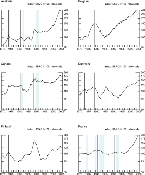
Source:  BIS. House prices are defined by PCE deflators. Business-cycle dates, except for the United States, were chosen by the Economic Cycle Research Institute (where available). Business cycle dates for the United States were chosen by the National Bureau of Economic Research. Vertical lines denote real house price peaks. Shaded areas denote recessions.

Data for Chart 2.1

Date	Australia	Belgium	Canada	Denmark	Finland	France	Germany	Ireland	Italy	Japan	Netherlands	New Zealand	Norway	Spain	Sweden	Switzerland	United Kingdom	United States
1970.03.01	78.06	100.90	88.08	89.62	87.25	94.55	91.77	82.06	78.23	69.35	103.61	97.23	89.17	-	138.77	84.43	68.98	83.70
1970.06.01	78.63	99.81	87.54	88.26	90.68	93.86	94.70	92.55	77.93	71.25	105.58	98.38	90.97	-	137.27	83.68	68.24	83.37
1970.09.01	80.32	98.34	88.01	85.82	92.92	92.77	96.87	99.78	77.14	73.95	108.62	98.49	89.65	-	134.57	85.27	70.78	83.89
1970.12.01	80.97	96.51	90.16	84.89	94.05	91.39	98.41	101.50	75.98	74.81	109.58	97.15	90.84	-	133.16	85.93	68.69	83.82
1971.03.01	81.45	94.36	90.08	92.33	91.86	90.00	98.65	99.15	78.57	76.43	107.96	98.27	86.86	84.64	138.42	89.87	68.70	85.32
1971.06.01	81.95	93.07	90.02	90.95	89.59	88.66	99.60	96.79	77.85	78.25	109.57	98.40	88.28	85.53	133.13	87.72	68.80	86.69
1971.09.01	83.60	92.60	88.81	92.27	88.14	89.06	100.06	96.24	76.95	80.28	113.86	98.50	87.70	84.50	129.05	90.53	72.75	86.74
1971.12.01	84.94	92.92	92.23	95.58	88.05	90.50	100.43	96.54	76.85	81.41	114.83	99.05	88.32	84.52	129.37	91.52	74.69	88.29
1972.03.01	85.45	94.00	93.33	100.01	88.18	93.02	99.72	97.56	77.48	83.31	113.31	100.97	86.26	82.02	132.21	94.32	78.11	87.62
1972.06.01	86.05	95.35	92.36	102.26	87.99	94.74	100.66	98.68	82.79	84.25	113.10	104.19	86.93	83.36	134.63	98.21	85.05	89.59
1972.09.01	87.19	96.96	92.11	101.61	90.53	95.58	100.80	97.99	77.12	86.05	114.35	105.52	85.10	84.34	133.16	101.36	95.41	90.54
1972.12.01	90.50	98.84	95.29	103.90	94.36	95.86	100.81	98.04	75.90	90.86	114.88	109.06	86.36	84.95	134.16	104.60	99.84	91.76
1973.03.01	91.71	100.98	98.63	107.11	97.95	96.90	100.46	95.21	78.52	96.80	114.98	112.82	84.67	84.99	133.76	110.08	109.44	94.64
1973.06.01	94.37	102.45	101.51	106.58	101.18	97.41	100.49	94.47	76.17	101.78	115.95	118.09	87.51	89.41	134.17	106.31	113.54	95.10
1973.09.01	98.82	103.24	106.46	109.25	102.19	98.13	101.60	95.48	70.00	106.76	118.07	123.94	87.37	93.34	132.30	108.99	118.32	95.77
1973.12.01	101.91	103.39	114.21	108.05	104.59	100.14	101.15	97.15	75.19	109.06	119.30	132.33	90.18	96.16	132.35	103.74	114.76	95.85
1974.03.01	106.19	102.95	123.28	103.84	105.16	100.92	101.77	97.88	89.43	105.10	119.80	143.88	88.07	100.83	133.83	100.45	110.76	95.37
1974.06.01	105.26	102.48	124.73	96.68	103.85	101.34	101.25	97.85	101.69	103.54	119.56	154.53	92.49	108.04	129.71	98.57	106.13	94.56
1974.09.01	101.07	101.95	119.84	94.27	101.73	101.16	101.31	99.46	111.90	100.77	119.18	158.26	93.12	108.36	126.21	97.04	103.45	94.58
1974.12.01	98.48	101.35	116.09	97.44	98.79	100.37	99.54	100.28	113.13	94.45	118.75	157.07	95.39	104.62	137.15	94.34	99.16	92.82
1975.03.01	97.91	100.68	119.27	102.24	95.64	99.18	98.39	97.90	108.41	89.33	118.31	153.52	92.49	100.66	137.59	88.31	93.95	93.56
1975.06.01	98.34	101.50	120.79	103.46	93.05	99.34	97.25	99.09	104.60	86.35	121.40	147.54	93.15	113.31	140.40	85.33	90.55	93.89
1975.09.01	97.67	103.74	121.20	106.85	90.74	99.97	96.95	99.33	100.65	85.50	122.78	143.94	90.80	119.58	140.15	84.42	90.07	91.56
1975.12.01	95.39	107.34	123.35	107.49	89.04	101.09	96.98	98.72	100.34	84.00	126.64	141.86	93.01	120.18	142.28	83.40	87.04	91.48
1976.03.01	96.26	112.28	126.18	107.55	88.14	102.58	97.55	97.35	101.96	82.04	131.14	138.30	89.13	114.85	143.98	80.43	85.68	91.76
1976.06.01	96.12	116.95	125.50	104.67	87.24	103.78	98.47	96.11	104.05	80.22	143.99	135.51	92.56	112.81	147.54	80.81	86.18	93.79
1976.09.01	94.01	121.34	123.68	105.14	85.85	105.32	99.45	93.89	107.65	79.42	152.88	132.55	91.82	113.10	151.93	79.31	85.68	93.35
1976.12.01	93.96	125.41	126.45	105.49	84.17	106.42	100.50	99.50	110.04	78.66	159.39	131.25	95.72	115.52	146.96	81.45	83.04	93.55
1977.03.01	94.24	129.16	124.26	104.72	82.46	108.48	100.95	96.21	111.92	77.84	172.99	130.80	92.84	119.89	151.64	79.97	79.40	94.62
1977.06.01	94.10	132.60	122.20	108.72	80.34	108.91	102.07	99.07	111.32	77.48	194.14	127.23	93.56	123.61	154.74	81.10	78.50	96.60
1977.09.01	92.37	135.73	118.86	110.76	78.63	109.49	103.36	103.66	107.58	77.30	198.02	123.79	92.48	127.16	154.50	81.72	79.02	97.50
1977.12.01	91.81	138.61	120.14	111.89	77.57	110.17	105.10	105.11	105.19	77.70	196.06	119.10	94.33	132.32	153.92	80.69	80.62	99.34
1978.03.01	93.28	141.24	117.22	113.90	76.67	111.15	106.64	116.02	103.97	77.60	197.56	117.22	90.39	139.20	151.20	80.82	79.73	100.73
1978.06.01	90.86	143.89	118.57	116.23	77.05	110.76	108.07	123.31	104.85	77.74	209.20	114.85	90.45	142.12	157.45	82.70	81.93	102.15
1978.09.01	89.51	146.56	115.63	117.10	74.13	110.84	109.55	124.16	107.49	77.95	195.24	113.05	90.71	141.60	159.53	84.11	85.62	103.44
1978.12.01	87.64	149.25	118.20	116.23	74.12	111.03	111.65	119.83	113.73	79.11	190.57	111.54	90.62	138.67	155.93	86.66	89.39	104.52
1979.03.01	90.81	151.98	119.89	116.87	74.36	111.74	112.63	125.19	123.38	80.45	183.39	110.92	89.04	133.52	157.99	86.81	91.61	107.41
1979.06.01	94.52	153.57	119.51	117.81	74.18	112.77	113.34	134.33	124.27	81.48	184.49	107.63	90.42	128.90	162.90	85.59	96.38	107.43
1979.09.01	94.20	154.05	116.49	114.35	74.23	114.03	113.17	128.82	117.49	82.61	179.20	103.65	89.37	124.66	165.08	85.85	97.00	107.20
1979.12.01	93.71	153.43	118.91	112.34	73.91	116.30	112.34	123.08	109.64	83.67	169.97	100.93	89.17	121.13	155.87	88.22	99.08	106.75
1980.03.01	92.90	151.76	117.89	107.30	76.13	118.26	111.46	127.63	100.60	84.34	162.72	99.27	89.28	119.17	147.42	91.90	99.88	105.66
1980.06.01	95.61	149.58	119.45	102.30	76.42	120.67	110.38	128.08	104.02	85.53	159.57	98.41	91.49	115.52	149.81	90.13	99.89	104.21
1980.09.01	96.42	146.29	121.01	101.56	77.69	121.73	111.46	128.64	117.82	87.06	148.71	98.26	90.10	114.48	143.71	91.88	102.23	105.27
1980.12.01	97.48	141.59	124.79	99.39	75.39	122.35	112.25	128.46	130.51	88.50	144.54	97.66	90.40	111.43	138.22	90.98	99.11	103.22
1981.03.01	101.25	136.51	125.48	95.24	78.22	123.03	113.80	125.37	144.67	89.63	140.50	98.73	88.49	110.30	133.27	93.62	97.02	101.57
1981.06.01	102.54	135.11	123.34	88.51	77.59	122.04	113.46	123.89	146.11	91.07	134.98	99.59	89.46	105.56	130.09	95.71	97.24	101.72
1981.09.01	98.54	133.05	123.32	83.59	78.67	119.84	113.89	123.32	137.11	92.37	128.35	100.83	87.46	103.49	125.93	94.80	96.56	101.45
1981.12.01	100.54	133.06	122.79	82.33	78.85	117.62	113.72	121.33	131.63	93.61	116.66	103.56	86.83	98.52	121.11	94.77	91.85	100.11
1982.03.01	97.33	122.11	115.12	79.40	83.34	115.98	114.17	120.07	131.86	95.10	110.81	105.54	86.59	95.18	119.30	96.92	88.18	100.22
1982.06.01	97.85	119.43	107.09	78.97	83.68	113.12	112.82	119.18	134.13	96.54	110.59	105.98	87.84	93.30	119.77	94.12	90.39	99.73
1982.09.01	93.03	123.08	102.61	75.81	84.84	112.66	111.66	115.31	136.68	97.12	112.45	108.18	86.72	93.56	118.47	93.13	91.40	97.75
1982.12.01	90.34	121.93	102.58	75.39	87.42	111.56	111.24	114.07	133.76	97.52	106.85	107.98	85.00	94.90	112.38	93.06	90.41	97.37
1983.03.01	90.75	113.31	108.38	80.83	92.47	109.77	111.14	111.64	127.59	98.63	106.64	108.59	86.37	99.21	110.73	93.45	92.60	98.44
1983.06.01	92.14	112.02	107.09	90.05	92.84	107.55	109.64	108.81	123.59	99.21	111.37	107.94	87.02	99.94	108.94	93.87	94.69	98.65
1983.09.01	90.42	111.33	103.77	90.26	94.60	105.72	108.16	108.48	121.96	99.37	111.76	107.89	85.06	100.88	104.90	96.08	97.44	98.04
1983.12.01	92.39	108.49	102.93	90.79	96.91	103.67	107.08	103.42	116.76	99.36	106.04	108.35	82.67	100.48	102.87	96.29	97.16	97.81
1984.03.01	94.14	105.97	101.59	94.45	99.22	101.81	105.70	104.38	111.90	99.26	104.96	107.12	85.69	98.37	101.69	97.09	96.87	98.26
1984.06.01	95.18	105.44	101.53	95.00	97.82	100.76	104.07	103.71	109.29	99.63	105.90	105.82	89.81	96.74	103.77	98.15	98.24	98.96
1984.09.01	97.80	106.35	98.65	94.76	98.99	100.09	103.17	102.94	108.33	99.97	107.69	105.08	93.44	96.63	103.68	98.01	101.09	99.18
1984.12.01	96.39	104.00	99.14	97.70	98.00	99.99	101.58	100.71	105.13	99.86	105.06	104.41	96.67	97.93	102.21	97.09	101.43	99.61
1985.03.01	100.00	100.00	100.00	100.00	100.00	100.00	100.00	100.00	100.00	100.00	100.00	100.00	100.00	100.00	100.00	100.00	100.00	100.00
1985.06.01	98.47	99.26	101.02	103.61	97.41	100.51	99.11	100.47	96.83	100.29	105.00	96.72	101.10	98.72	101.37	98.38	102.17	100.99
1985.09.01	98.89	104.51	100.71	111.22	96.20	101.11	99.03	99.90	96.10	100.50	104.76	96.05	104.40	99.32	100.43	99.96	103.09	102.17
1985.12.01	98.64	102.24	104.31	113.49	96.53	102.05	98.58	101.10	95.02	100.64	104.43	97.13	111.32	98.52	98.55	99.78	105.53	102.86
1986.03.01	99.21	100.43	108.32	120.53	98.83	103.52	99.16	99.12	94.88	100.88	103.75	97.79	123.54	97.54	99.07	104.00	106.77	104.14
1986.06.01	100.21	102.80	113.29	117.81	97.49	104.76	100.11	100.77	94.22	101.37	107.73	97.85	129.06	100.07	99.06	102.07	110.78	106.34
1986.09.01	94.82	108.74	113.98	113.68	97.26	106.42	100.24	101.48	93.17	102.07	112.28	94.97	129.83	106.34	100.40	104.05	114.36	107.63
1986.12.01	93.84	107.42	120.49	113.36	99.23	108.09	99.40	99.54	93.41	103.20	109.36	93.05	129.78	113.85	101.78	105.01	116.73	108.87
1987.03.01	93.15	106.43	129.23	105.62	101.46	109.58	98.29	98.38	95.36	104.45	110.61	101.24	123.71	129.22	105.40	106.98	118.08	110.08
1987.06.01	92.40	105.84	126.60	103.98	103.49	111.43	97.69	96.76	96.16	106.50	113.60	100.78	132.69	135.68	106.11	109.25	122.84	111.18
1987.09.01	92.00	110.15	125.70	102.01	106.35	113.25	97.92	99.00	95.76	110.23	114.80	100.11	128.06	140.27	107.21	110.81	127.83	111.92
1987.12.01	94.71	108.32	131.25	100.25	111.05	115.32	97.96	103.24	96.86	112.53	113.24	98.63	126.10	145.32	109.23	111.67	134.33	112.01
1988.03.01	97.10	109.14	142.17	100.77	123.43	117.42	98.63	101.22	99.97	113.00	113.28	99.35	127.34	154.08	114.65	116.80	137.61	113.02
1988.06.01	100.21	113.08	143.71	99.98	129.74	119.14	99.05	100.16	99.48	113.67	117.06	96.54	125.47	157.72	116.76	119.82	143.73	114.17
1988.09.01	108.88	116.56	143.40	100.92	139.17	120.66	99.59	102.24	95.54	114.51	120.42	97.35	124.28	176.81	121.88	123.44	160.68	114.05
1988.12.01	117.98	114.70	153.31	100.51	151.56	122.27	99.78	104.49	101.28	115.77	118.13	96.25	122.16	168.99	123.15	131.23	168.88	114.14
1989.03.01	125.25	116.38	167.79	98.10	160.95	123.40	99.46	107.91	116.52	117.34	119.32	94.61	118.49	180.83	128.60	132.55	169.40	114.27
1989.06.01	126.05	119.86	150.80	97.07	162.60	124.66	99.58	105.27	122.99	117.94	123.40	94.02	114.05	187.53	131.68	134.08	172.67	114.32
1989.09.01	124.67	123.21	152.49	94.13	159.91	126.13	100.52	109.43	121.69	119.48	126.03	93.26	108.12	194.37	135.30	134.41	176.30	116.21
1989.12.01	123.28	124.61	160.08	92.11	154.35	127.64	101.48	116.80	126.49	122.99	123.88	92.14	105.18	195.88	133.57	135.11	169.99	116.34
1990.03.01	122.58	126.94	155.69	87.52	147.11	129.34	102.80	121.11	138.08	126.76	122.40	92.37	102.12	205.61	136.36	132.69	163.91	115.12
1990.06.01	121.07	126.60	143.89	87.22	145.30	130.58	103.92	119.45	142.96	130.97	126.50	91.83	101.85	204.32	135.54	129.46	158.15	113.82
1990.09.01	118.12	130.17	142.98	84.52	141.82	131.39	103.89	122.53	141.13	134.97	123.51	91.68	98.28	207.03	135.41	127.00	157.95	112.74
1990.12.01	116.59	130.34	142.19	83.45	134.47	131.60	104.24	119.32	142.66	137.45	119.69	90.32	92.82	206.15	131.17	122.74	152.54	110.78
1991.03.01	115.29	130.17	145.78	84.41	123.18	131.74	104.88	121.34	147.66	137.31	117.85	89.85	91.41	216.80	133.84	120.04	148.33	110.79
1991.06.01	116.61	130.09	149.87	84.83	120.02	131.53	104.99	116.78	149.48	137.38	122.89	90.23	90.26	219.08	130.38	119.31	143.05	110.63
1991.09.01	118.95	135.27	140.35	83.99	113.53	130.44	104.47	118.96	148.95	136.58	123.85	90.14	88.66	220.85	130.24	120.42	143.80	109.85
1991.12.01	117.92	137.32	142.68	84.36	106.33	128.70	103.91	122.22	149.75	135.06	123.95	90.69	86.77	227.11	127.33	116.38	140.67	110.43
1992.03.01	117.44	136.76	144.27	83.45	102.58	127.05	105.03	122.32	151.60	132.80	125.69	90.01	84.20	212.42	121.35	113.53	136.58	110.33
1992.06.01	116.74	142.07	144.72	82.97	96.15	125.38	105.45	119.85	152.34	130.39	123.70	90.02	84.00	206.06	119.24	112.00	131.73	109.38
1992.09.01	116.14	146.51	143.87	80.87	88.65	124.12	106.17	120.00	152.10	128.54	132.39	89.40	83.40	200.29	115.77	107.60	132.04	109.74
1992.12.01	116.78	145.16	146.25	78.70	82.74	123.05	106.68	119.54	150.66	126.94	131.13	89.80	79.56	199.83	105.84	105.78	125.93	109.47
1993.03.01	116.55	141.85	146.79	77.33	79.57	121.89	105.93	116.64	149.64	124.42	130.56	89.03	77.00	194.30	97.88	103.56	125.60	108.73
1993.06.01	117.11	148.32	145.84	76.50	79.80	121.07	106.13	119.41	147.39	123.03	134.91	90.30	80.46	194.81	96.59	102.62	125.04	108.93
1993.09.01	116.72	151.09	142.10	79.57	80.59	120.48	106.46	120.41	143.38	121.65	139.52	92.35	83.05	193.48	94.86	99.08	126.97	109.17
1993.12.01	117.24	152.14	142.53	83.28	82.96	119.85	106.64	117.58	139.90	121.03	139.02	93.41	85.17	191.58	95.49	99.16	123.72	109.43
1994.03.01	118.61	149.72	149.47	87.42	84.54	119.47	106.66	122.18	137.07	119.71	141.01	94.29	87.84	187.50	96.90	101.08	124.86	109.54
1994.06.01	119.44	156.68	148.14	86.71	85.89	118.58	106.95	119.76	134.75	119.03	144.07	94.96	90.05	186.24	99.08	101.29	125.56	109.25
1994.09.01	121.16	160.04	145.07	85.09	84.86	117.50	106.89	117.02	132.45	118.63	150.42	97.90	93.46	185.97	99.08	100.68	127.66	108.58
1994.12.01	120.26	158.29	146.37	85.63	83.95	116.06	106.66	122.87	130.80	118.00	146.44	100.90	92.31	183.84	96.65	98.77	125.92	107.80
1995.03.01	120.58	152.48	141.96	87.17	83.06	114.24	106.34	126.49	129.93	117.69	146.47	102.06	92.64	183.75	95.95	97.25	122.65	107.69
1995.06.01	118.76	159.92	137.68	89.91	82.02	112.95	106.04	123.88	128.16	117.72	149.27	101.76	95.37	183.66	97.06	96.20	123.30	108.95
1995.09.01	118.02	163.70	138.80	92.21	80.15	111.59	105.77	123.91	126.55	117.28	154.92	102.10	96.80	183.76	95.49	94.78	123.78	110.17
1995.12.01	117.09	163.78	138.83	94.70	79.35	110.70	105.39	128.00	124.30	116.74	153.70	103.13	97.15	182.57	93.56	92.78	121.41	110.58
1996.03.01	116.86	159.54	136.69	95.39	80.77	110.09	105.04	129.15	122.08	116.12	155.86	104.24	98.75	181.52	93.84	91.19	121.96	111.21
1996.06.01	117.54	164.38	138.49	97.02	82.51	109.35	104.49	133.26	119.50	115.44	159.15	105.69	102.05	181.11	94.99	89.79	120.87	110.62
1996.09.01	117.69	166.86	135.97	99.48	84.99	109.04	104.00	142.17	117.46	114.97	166.67	105.51	103.13	180.31	95.47	89.66	124.66	110.58
1996.12.01	117.16	163.95	136.05	102.92	88.03	108.34	103.08	143.00	114.58	114.35	167.57	105.46	104.51	179.02	95.95	87.16	126.28	110.80
1997.03.01	117.63	162.79	137.20	105.09	94.37	107.48	101.62	144.42	111.55	114.12	168.25	104.07	104.58	178.33	96.70	86.11	127.77	111.30
1997.06.01	119.29	166.59	140.13	107.02	96.82	113.65	100.69	155.45	109.76	112.17	173.77	104.02	112.03	179.07	99.79	85.08	129.13	111.99
1997.09.01	120.53	171.24	137.51	108.93	97.52	113.44	99.35	159.37	109.36	111.98	179.72	103.69	112.61	178.59	100.60	85.13	134.43	113.36
1997.12.01	122.32	168.26	136.72	109.40	99.42	112.03	98.69	171.50	109.18	111.71	180.10	104.23	113.39	178.70	100.78	84.76	132.93	114.48
1998.03.01	124.96	168.23	135.17	111.21	102.57	110.34	98.46	176.44	109.46	111.65	182.07	104.01	115.50	178.67	103.79	85.12	135.45	116.11
1998.06.01	127.37	170.31	135.92	115.72	104.09	115.79	97.74	183.60	109.37	111.26	185.70	103.49	122.18	181.77	107.33	85.23	141.40	116.86
1998.09.01	127.17	180.08	132.76	117.39	106.01	117.58	97.64	184.31	109.00	111.10	192.85	102.29	120.00	184.43	109.83	84.69	147.05	118.08
1998.12.01	129.07	178.93	134.09	118.64	106.40	115.88	98.10	199.84	109.60	110.18	195.13	102.39	116.15	186.87	111.21	84.51	145.57	119.02
1999.03.01	131.00	177.89	134.37	119.40	108.38	117.37	98.94	207.50	111.01	110.37	196.51	102.37	120.31	190.11	112.26	85.20	146.15	119.99
1999.06.01	133.52	183.81	138.80	120.38	110.83	121.97	98.43	207.38	112.13	109.52	208.33	102.25	128.09	198.39	116.34	84.94	151.70	120.84
1999.09.01	135.79	190.83	136.82	121.86	114.46	128.17	98.72	217.06	113.36	108.29	220.92	102.35	128.51	197.66	118.97	84.26	159.97	122.08
1999.12.01	139.58	182.90	138.12	120.73	116.44	127.93	98.64	224.96	114.35	107.26	231.49	102.65	130.76	203.87	119.47	84.21	163.82	122.76
2000.03.01	141.51	183.21	138.24	122.17	117.01	130.63	98.58	227.77	115.53	106.74	235.85	102.53	136.37	209.66	122.49	83.83	167.27	124.21
2000.06.01	143.40	185.70	140.24	124.72	117.97	134.76	98.52	234.79	117.06	106.07	245.19	103.28	145.33	217.05	127.61	84.98	175.97	125.78
2000.09.01	139.67	189.30	138.94	126.81	114.38	138.70	98.04	232.96	119.20	105.48	257.71	102.32	139.92	223.48	131.23	85.94	178.85	127.64
2000.12.01	141.81	189.94	139.42	127.01	112.08	136.11	97.73	244.39	120.79	104.69	257.76	102.04	140.48	226.94	131.98	85.51	183.15	129.13
2001.03.01	143.75	189.10	139.08	128.91	110.92	138.49	97.81	247.46	122.38	104.01	254.68	103.06	143.18	235.54	135.00	86.30	180.89	131.39
2001.06.01	147.56	190.47	143.50	129.23	111.25	142.81	97.48	252.19	123.49	103.28	260.02	102.48	148.28	243.20	135.03	86.13	186.08	132.95
2001.09.01	155.31	196.44	143.80	129.95	110.15	146.18	97.50	236.98	125.18	102.68	264.52	102.53	148.84	248.51	136.51	86.87	191.90	134.99
2001.12.01	160.11	192.83	145.96	128.89	109.41	147.16	97.69	237.76	127.33	102.08	265.64	102.83	148.20	254.27	134.58	87.33	187.68	136.51
2002.03.01	165.19	195.89	151.76	129.87	112.86	150.62	97.68	244.80	129.53	101.02	265.75	103.44	152.40	264.66	136.29	88.30	192.78	138.54
2002.06.01	172.82	200.91	156.27	132.02	115.25	153.77	97.76	249.76	131.62	99.99	269.50	103.41	156.93	270.27	140.08	88.29	208.05	140.19
2002.09.01	178.42	208.16	153.11	131.87	115.75	159.02	97.56	250.54	133.60	99.13	275.36	103.95	150.17	283.69	144.80	89.53	221.59	142.52
2002.12.01	185.52	208.89	157.17	131.02	116.36	159.52	96.93	254.66	135.81	98.43	270.30	105.53	148.11	289.15	144.28	90.08	231.56	144.33
2003.03.01	190.64	206.15	159.81	130.22	117.80	165.21	95.96	261.45	138.34	97.46	267.78	106.47	148.47	299.86	143.45	89.83	234.39	145.15
2003.06.01	200.18	212.71	165.49	132.97	120.82	174.06	95.67	269.73	141.26	96.52	270.43	108.14	151.78	312.01	147.39	90.98	240.48	146.67
2003.09.01	206.71	220.23	168.37	134.47	123.25	179.57	95.31	273.97	143.89	95.22	270.49	110.10	150.75	320.52	148.05	91.91	245.71	148.54
2003.12.01	218.00	222.35	173.31	133.67	124.76	179.67	95.15	283.50	147.12	93.92	274.47	113.58	151.88	330.54	149.46	92.47	249.80	153.61
2004.03.01	223.08	-	175.02	135.50	125.88	-	-	284.04	150.90	92.29	275.89	115.28	164.24	342.76	152.61	92.59	251.16	154.61
2004.06.01	219.05	-	181.95	-	130.43	-	-	-	152.56	92.07	279.80	118.17	-	-	160.20	92.48	265.66	156.78

Chart 2.2:  International Co-movement of Real House Prices

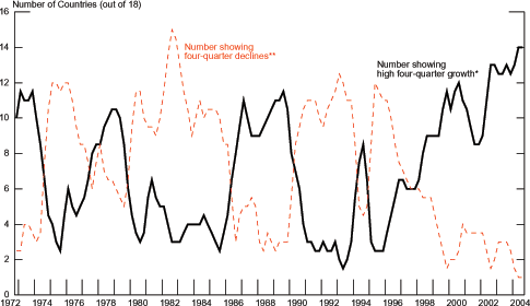
*  Two-quarter moving average of the number of countries experiencing high four-quarter growth rate of real house prices. High growth rate is defined as four-quarter growth rate greater than two times each country's average four-quarter growth rate between 1970 and 2004.
**  Two-quarter moving average of the number of countries experiencing negative four-quarter growth in real house prices.

Chart 2.3:  Ratio of Nominal House Prices to Disposable Income

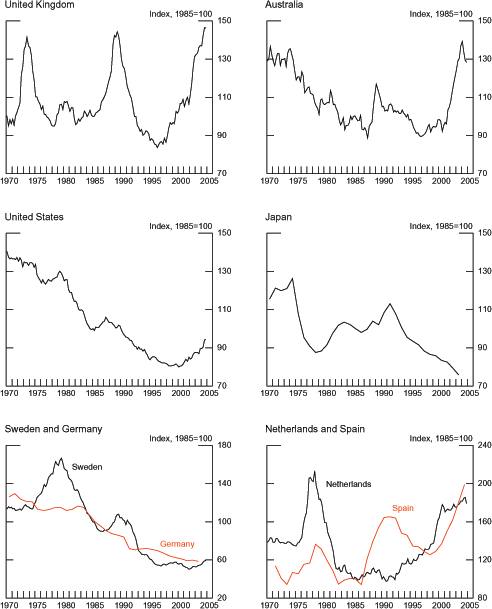
Chart 2.4:  Ratio of Nominal House Prices to Rents

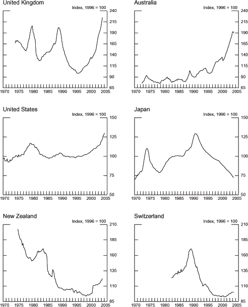
Chart 2.5:  Ratio of Nominal House Prices to Disposable Income

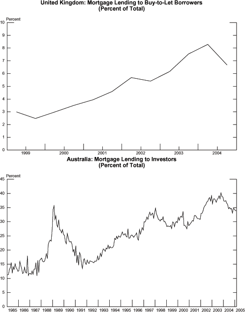
Chart 3.1:  Nominal Policy Interest Rates and Real House Prices (Median over Peaks)

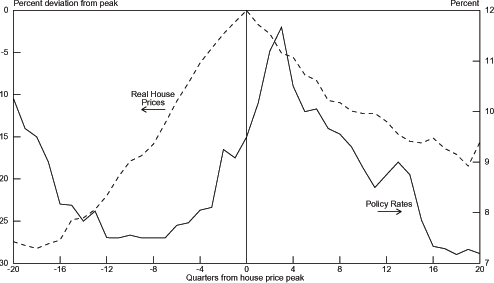
Chart 3.2:  CPI Inflation and Real House Prices (Median over All Peaks)

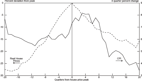
Chart 3.3:  Real GDP Growth and Real House Prices (Median over All Peaks)

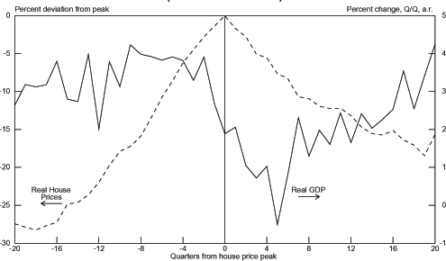
Chart 3.4:  Output Gap and Real House Prices (Median over All Peaks)

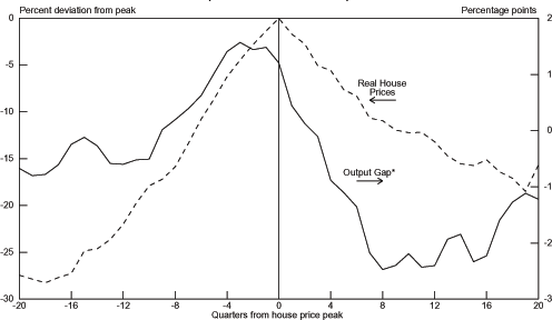
*  Output gaps are estimates from the OECD Economic Outlook, December 2004. Output gaps are expressed as the percentage that actual output is greater (positive gap) or less (negative gap) than its potential level.

Chart 3.5:  Real Consumption Growth and Real House Prices (Median over All Peaks)

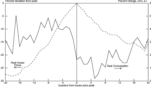
Chart 3.6:  Real Total Investment Growth and Real House Prices (Median over All Peaks)

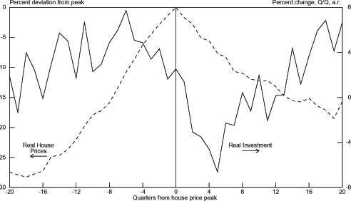
Chart 3.7:  Real Long-Term Interest Rates and Real House Prices (Median over Peaks)

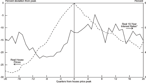
*  Real 10-year interest rates are staff estimates (see appendix)>

Chart 3.8:  M3 and Real House Prices (Median over Peaks)

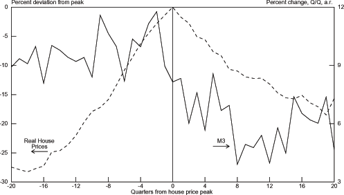
Chart 3.9:  Real Equity Prices and Real House Prices (Median over All Peaks)

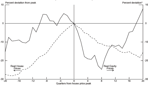
*  Deviation normalized to zero at house price peak date.

Chart 3.10:  Budget-Balance-to-GDP Ratio and Real House Prices (Median over Peaks)

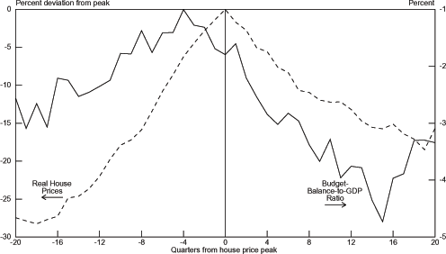
Chart 3.11:  Current-Account-to-GDP Ratio and Real House Prices (Median over Peaks)

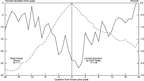
Chart 3.12:  Real House Prices, Nominal Policy Rate, and Inflation

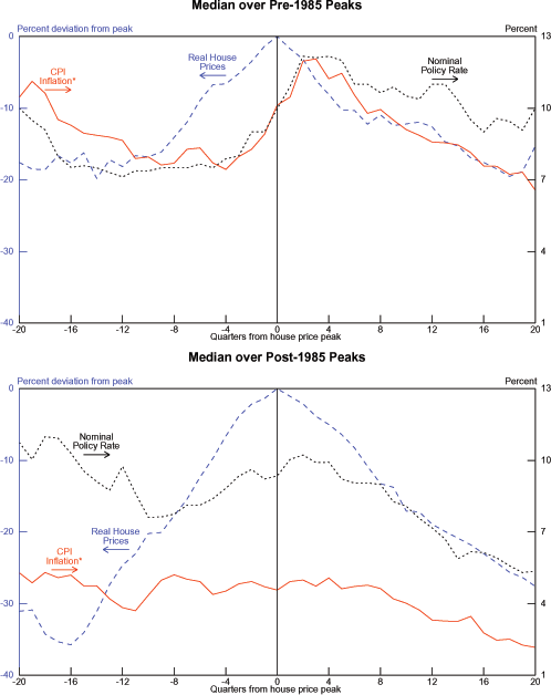
*  Four-quarter percent change.

Chart 3.13:  Population Growth (Annual Growth in Working Age Population, 15-64 years)

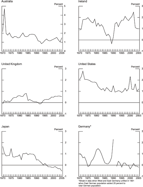
*  Germany: Break in data when West and East Germany unified in 1991 when East German population added 25 percent to total German population.

Chart 3.14:  Nominal Policy Interest Rates and Real House Prices (Median)

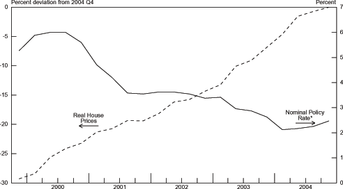
Chart 3.15:  CPI Inflation and Real House Prices (Median)

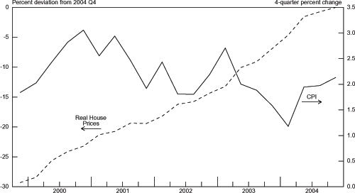
*  In calculating the median nominal policy rate, we included the euro area countries as one observation.

Chart 3.16:  Real GDP Growth and Real House Prices (Median)

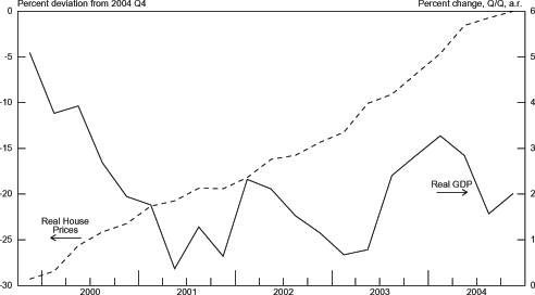
Chart 3.17:  Output Gap and Real House Prices (Median)

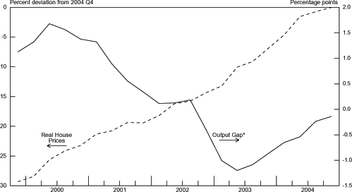
*  Output gaps are estimates from the OECD Economic Outlook, December 2004. Output gaps are expressed as the percentage that actual output is greater (positive gap) or less (negative gap) than its potential level.

Chart 3.18:  Real Consumption Growth and Real House Prices (Median)

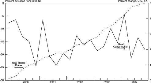
Chart 3.19:  Real Total Investment Growth and Real House Prices (Median)

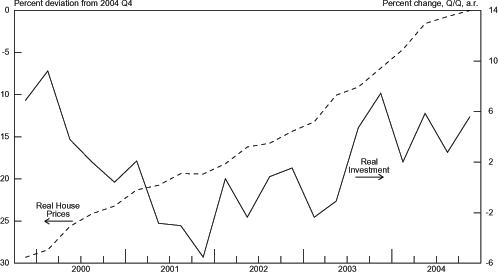
Chart 3.20:  Long-Term Interest Rates and Real House Prices (Median)

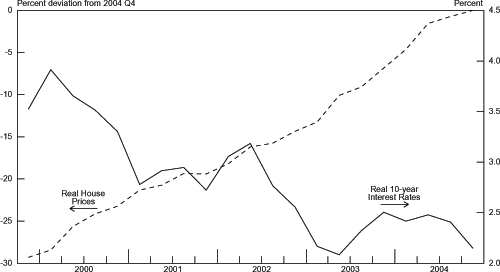
Chart 3.21:  M3 and Real House Prices (Median)

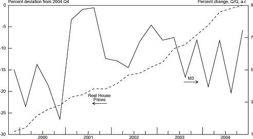
Chart 4.1:  Policy Rate, Output Gaps and Inflation

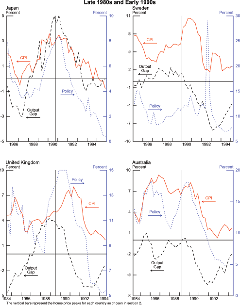
The vertical bars represent the house price peaks for each country as chosen in section 2.

Chart 4.2:  Real House Prices and Monetary Policy

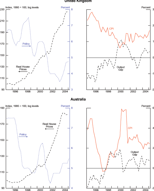
Chart 5.1:  U.K. Properties Taken into Possession

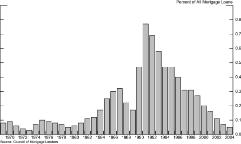
Source:  Council of Mortgage Lenders.

Chart 5.2:  European Residential Mortgage Backed Security Insurance

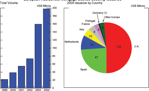
Chart 5.2:  Mortgage Securitization

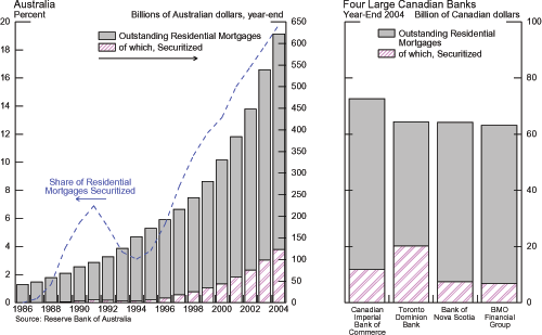
Source:  Reserve Bank of Australia.

Chart 5.3:  U.S. Exposure to Foreign Real Estate

Outstanding Real Estate Loans by Foreign Offices of U.S. Banks

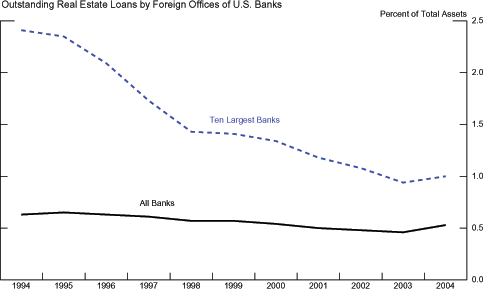
U.S. Holdings of Foreign Securities by Industry

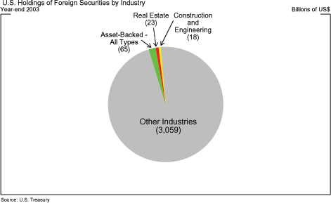
Source:  U.S. Treasury.

Chart 5.4:  Residential Construction and Real House Prices

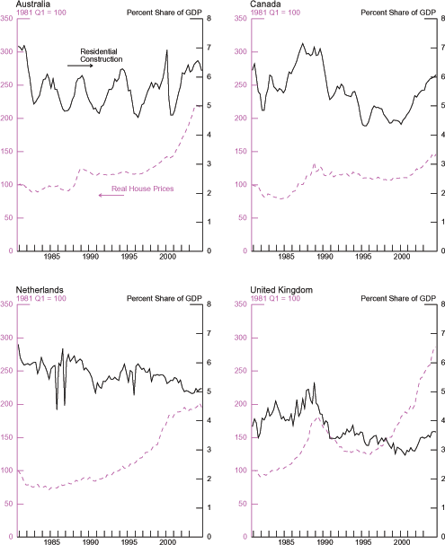
Chart 5.5:  Simulated House Price Shocks (Deviations from Baseline)

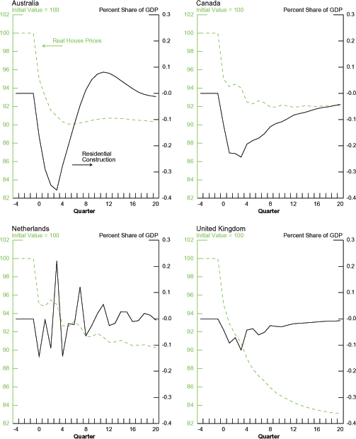
*  From a four-lag VAR in house prices and construction as a share of GDP estimated quarterly from 1971 to 2004.

Footnotes

*  The authors thank David Bowman, Sally Davies, Ellen Dykes, Jon Faust, Richard Freeman, William Helkie, Karen Johnson, Steven Kamin, Michael Leahy, Andreas Lehnert, Nathan Sheets, David Wilcox, and Paul Wood for helpful comments. Sebastien Bradley, Nathanael Clinton, Hilary Croke, Troy Dibley, Kristian Rogers, and Elizabeth Thomasson provided excellent research assistance. We thank Sebastian Wider of the Bundesbank for helpful information and Stephen Arthur and other staff of the Bank for International Settlements for the house price data. The views expressed in this paper are solely the responsibility of the authors and should not be interpreted as reflecting the views of the Board of Governors of the Federal Reserve System or of any other person associated with the Federal Reserve System. Emails: [email protected], [email protected], [email protected], [email protected], [email protected]. Return to text

1.  Our sample comprises Australia, Belgium, Canada, Denmark, Finland, France, Germany, Ireland, Italy, Japan, the Netherlands, New Zealand, Norway, Spain, Sweden, Switzerland, the United Kingdom, and the United States. Return to text

2.  Our data on house prices come from the Bank for International Settlements (BIS) and are derived from national sources (see data appendix and table A1). The frequency for which the house price data are available varies by country and over time. Both annual and semi-annual data are interpolated by the BIS to derive quarterly series. In addition, the data quality varies substantially among the countries, and for some countries the sample changes in significant ways over the time covered. For example, a close look at the series for Belgium, Italy, France, and Spain indicates significant differences between the volatility and trends in the early part of the series and those in the latter part of the series. These data issues led us to focus on the longer trends in house prices (such as the behavior around peak dates) rather than quarter-to-quarter movements in the indexes. Return to text

3.  One might infer from our data that real house price booms were more frequent in the pre-1985 sample than afterward, but this inference would be a mistake. Although we do not yet have enough data to identify the timing of the current peaks, it seems highly likely that we will find a large number of peaks ex post.  Return to text

4.  Our algorithm is fairly good at choosing the outstanding high points for each country. There are a few points chosen by this exercise, however, that do not appear, at least to the eye, to be significant. For example, the algorithm picks out a peak date in 1995 for Australia and one in 1994 for Germany; in both of these cases, the house price movements surrounding the peak are relatively flat. Return to text

5.  Otrok and Terrones (2005) show that a global factor is important for determining the movement of national real house prices. Return to text

6.  The ratio of house prices to disposable income is often referred to as an affordability measure. Such a ratio may have relevance for an individual household, but it is much less meaningful for the economy as a whole. Disposable income is a measure for the population as a whole whereas house prices are generally median selling prices for owner-occupied housing. Therefore, systematic differences in incomes among owners, potential owners, and non-owners affect the information content of this variable, as does the distribution of income for any of these groups. Return to text

7.  For example, flipping--buying a house with the sole intention of reselling for a profit--or buying rental property, even when rents are low relative to prices, may rise in anticipation of future rises in prices. Some have suggested that in these circumstances a spiral of self-fulfilling expectations and accelerating house prices becomes more likely. Return to text

8.  Investment properties are more likely to return to the market because they are relatively liquid. Transaction costs are smaller for investors than for owner-occupiers because investors do not have to move when they sell their property. In addition, investor sales increase the supply of housing without increasing demand, whereas an owner-occupier who sells his house must either purchase or rent another home. Investors may also choose simply to exit the market for a period of time. Return to text

9.  We also calculated the mean value of these indicators across all the peaks. The paths for median and mean values were roughly similar. Return to text

10.  The results of regression analysis (not shown) also point to the pro-cyclical nature of house prices and suggest monetary policy may play a role in house price movements. Return to text

11.  This estimate is derived using data from surveys of professional economic analysts taken from Consensus Forecasts. Return to text

12.  Girouard and Blöndal (2001) are among those making the argument that mortgage market deregulation played an important role in the house price swings that occurred in many countries in the late 1980s. Return to text

13.  Glaeser and Gyourko (2002) make this argument for the United States. They argue that the addition of zoning regulation in many cities across the United States has had a first-order impact on the rate of house price increases. Return to text

14.  Variable-rate loans typically have a lower interest rate than do fixed-rate loans because the household takes on some of the interest-rate risk. Return to text

15.  We exclude Germany and Japan because real house prices in both countries have been declining in recent years. Return to text

16.  Bank of England (various issues, 1987-90), Quarterly Bulletin, and the Financial Times (various issues, 1989). For Australia see Fraser (1991), Phillips (1988, 1990), and Johnston (1989). For Japan, see Yamaguchi (1999, 2002), Cargill, Hutchison, and Ito (1997), and Ahearne and others (2002). For Sweden, see Sveriges Riksbank (1990, 1991); Quarterly Review, Lindberg and Lindenius (1991); and Ringström (1987). Return to text

17.  Bank of England (1989), Quarterly Bulletin, August. Return to text

18.  Johnston (1989) does not specify whether these financial developments include house prices. Return to text

19.  From the MPC minutes, May 2004: "In presenting its decision to raise the repo rate, it would be important for the Committee to make clear that this did not imply that it was targeting house price inflation, or any other asset price. The significance of the unexpected acceleration in house prices was that it supported a stronger short-term outlook for consumption and output growth, and hence a steeper projected rise in inflation." Also see King (2004), Lomax (2004), and Barker (2005).  Return to text

20.  Bernanke and Gertler (2001) and Gruen, Plumb, and Stone (2003). The European Central Bank (2005) outlines a similar view its position but also emphasizes that its "two-pillar" strategy helps it identify "excess liquidity." Return to text

21.  The CPI, known elsewhere in Europe as the Harmonized Index of Consumer Prices, is also the inflation measure used by the European Central Bank. Return to text

22.  This minority likely included Andrew Large, who most often voted for higher rates during this period and who outlined his views in a speech last year (Large, 2004).  Return to text

23.  From the MPC minutes, June 2004: "...for some members, the need for a repo rate increase was reinforced by the prospect of higher domestic debt service levels... A further increase in interest rates now might encourage a more prudent approach towards incurring higher levels of prospective debt servicing, so helping to contain the vulnerability of demand to subsequent shocks." Return to text

24.  See Selody and Wilkins (2004), Gjedrem (2003), Bollard (2004), and Srejber (2005). This position has also been explored in Cecchetti, Genberg, and Wadhwani (2003). Issing (2003) also argues that, while he is skeptical of the argument, he "would... not completely disregard the possibility that situations of financial instability can be approximately identified in a relevant time horizon and that this information should find its way into policy decisions." Return to text

25.  The European Central Bank (2005) emphasizes that the ECB position is focused solely on inflation, but that its "medium-term orientation... reduces the risk [of] overlook[ing] risks to price stability at longer horizons." Return to text

26.  Bell (2005) arguably makes the same point.  Return to text

27.  Because national central banks in the euro area have no country-specific interest rate instrument, they may have a particular interest in the role of supervisory authorities. Wellink (2002) has noted the importance of bank supervision in the Netherlands.  Return to text

28.  In Macfarlane (2004): "The incentives in the mortgage distribution system have changed in such a way that there has been a step-by-step reduction in credit standards over recent years... I am not suggesting we have an urgent problem on our hands, but if present trends continue we could well have one in a few years." Return to text

29.  The Bundesbank (2002) notes that historically the tradeoff between renting and owning in Germany has been distorted by generous depreciation allowances for rental properties. Return to text

30.  This list is almost certainly not exhaustive because data on mortgage lending were not available from either Worldscope or Bloomberg for some larger non-U.S. banks. Return to text

31.  However, under typical securitization arrangements, such as those used by Fannie Mae and Freddie Mac, loans can (and regularly do) revert to the originator if information in the loan documentation is discovered later to be inaccurate.  Return to text

32.  In Germany, bank-issued Pfandbriefe, which are often referred to as "mortgage bonds," constitute the largest and most liquid market for private-sector debt securities. However, Pfandbriefe are so-called covered bonds, which besides being secured by a mortgage portfolio are also senior liabilities of the bank as a whole. In contrast, RMBS are somewhat riskier, with an investor's claim limited to a mortgage pool held by a special-purpose entity.  Return to text

33.  Spanish banks are also relatively active in securitization but reportedly have often retained significant quantities of the securities.  Return to text

34.  Any cross-border portfolio security investments by U.S. banks would also be included in these figures, but they are not a significant share of cross-border portfolio investment in practice. Return to text

35.  Because the estimated correlation of residuals between the two equations is positive for each country, prices are assumed to have a contemporaneous effect on construction in the VAR ordering. For these countries, a 5 percent quarterly price decrease represents a shock ranging from about 1.9 to 2.7 standard deviations. Return to text

36.  These figures almost certainly understate the impact on construction of a housing demand shock because they are estimated over a period that includes a mix of different shocks in each country. Return to text

This version is optimized for use by screen readers. Descriptions for all mathematical expressions are provided in LaTex format. A printable pdf version is available. Return to text

Home | Economic research and data | Publications and education resources
Accessibility | Contact us
Last update: August 26, 2008