
Board of Governors of the Federal Reserve System
International Finance Discussion Papers
Number 854, January 2006-Screen Reader Version*
Fully Modified Estimation with Nearly Integrated Regressors
NOTE: International Finance Discussion Papers are preliminary materials circulated to stimulate discussion and critical comment. References to International Finance Discussion Papers (other than an acknowledgment that the writer has had access to unpublished material) should be cleared with the author or authors. Recent IFDPs are available on the Web at http://www.federalreserve.gov/pubs/ifdp/. This paper can be downloaded without charge from the Social Science Research Network electronic library at http://www.ssrn.com/.
Abstract:
I show that the test procedure derived by Campbell and Yogo (2005, Journal of Financial Economics, forthcoming) for regressions with nearly integrated variables can be interpreted as the natural t-test resulting from a fully modified estimation with near-unit-root regressors. This clearly establishes the methods of Campbell and Yogo as an extension of previous unit-root results.
JEL classification: C22
Keywords: Fully modified estimation; Near-unit-roots; Predictive regressions.
1 Introduction
In the recent past, there has been much effort spent on the econometric analysis of forecasting regressions with nearly persistent regressors. Using Monte Carlo simulations, Mankiw and Shapiro (1986) showed in an influential paper that when the regressor variables in a predictive regression are almost persistent and endogenous, test statistics will no longer have standard distributions. Since then, a much better understanding of this phenomenon has been established and several alternative methods have been proposed; e.g. Cavanagh et al. (1995), Stambaugh (1999), Jansson and Moreira (2004), Lewellen (2004), and Campbell and Yogo (2005).
The issues encountered when performing inference in forecasting regressions with near-persistent variables are, of course, similar to those in the cointegration literature where the regressors are assumed to follow unit-root processes. Indeed, the case with nearly persistent regressors can be seen as a generalization of the standard unit-root setup.
In this note, I show that the efficient test for inference in predictive regressions derived by Campbell and Yogo (2005) can also be seen as the natural test resulting from a generalization of fully modified estimation (Phillips and Hansen, 1990, and Phillips, 1995) to the case of near-unit-root regressors. In addition, the optimality properties of the Campbell and Yogo (2005) test-statistic can be seen as a direct analogue of the optimal inference results derived by Phillips (1991) for cointegrated unit-root systems. These results firmly establish the link between current work on predictive regressions and earlier work on cointegration between unit-root variables.
2 Model and assumptions
Let the dependent variable be denoted ![]() , and the corresponding vector of
regressors,
, and the corresponding vector of
regressors, ![]() , where
, where
![]() is an
is an ![]() vector and
vector and ![]() . The behavior of
. The behavior of
![]() and
and ![]() are assumed to satisfy,
are assumed to satisfy,
where
1.
![]() , and
, and
![]()
2.
![]()
![]() and
and
![]()
3.
![]()
The model described by equations (1) and (2) and Assumption 1
captures the essential features of a predictive regression with
nearly persistent regressors. It states the usual martingale
difference (mds) assumption for the errors in the dependent
variables but allows for a linear time-series structure in the
errors of the predictors. The error terms ![]() and
and ![]() are also often highly
correlated. The auto-regressive roots of the regressors are
parametrized as being local-to-unity, which captures the
near-unit-root behavior of many predictor variables, but is less
restrictive than a pure unit-root assumption.
are also often highly
correlated. The auto-regressive roots of the regressors are
parametrized as being local-to-unity, which captures the
near-unit-root behavior of many predictor variables, but is less
restrictive than a pure unit-root assumption.
The local-to-unity parameter ![]() is generally unknown and not consistently estimable.
Following Campbell and Yogo (2005), I derive the results under the
assumption that
is generally unknown and not consistently estimable.
Following Campbell and Yogo (2005), I derive the results under the
assumption that ![]() is known. Bonferroni type methods can
then be used to form feasible tests, as in Cavanagh et al. (1995)
and Campbell and Yogo (2005); such methods are extensively explored
in these papers and will not be further discussed here.
is known. Bonferroni type methods can
then be used to form feasible tests, as in Cavanagh et al. (1995)
and Campbell and Yogo (2005); such methods are extensively explored
in these papers and will not be further discussed here.
Let
![]() be the joint
innovations process. Under Assumption 1, by standard arguments,
be the joint
innovations process. Under Assumption 1, by standard arguments,
![]() where
where
![]()
![]() ,
,
![]() ,
,
![]() ,
,
![]() ,
and
,
and
![]() denotes an
denotes an ![]() dimensional Brownian motion. Also, let
dimensional Brownian motion. Also, let
![]() be the one-sided long-run variance of
be the one-sided long-run variance of ![]() . The following lemma sums up the
key asymptotic results for the nearly integrated model in this
paper (Phillips 1987, 1988).
. The following lemma sums up the
key asymptotic results for the nearly integrated model in this
paper (Phillips 1987, 1988).
Analogous results hold for the demeaned variables
![]() ,
with the limiting process
,
with the limiting process ![]() replaced by
replaced by
![]() .
.
3 Fully modified estimation
Let
![]() denote the
standard OLS estimate of
denote the
standard OLS estimate of ![]() in equation (1). By Lemma 1 and the continuous
mapping theorem (CMT), it follows that
in equation (1). By Lemma 1 and the continuous
mapping theorem (CMT), it follows that
as
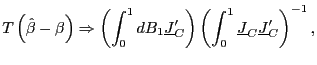
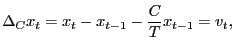
In the pure unit-root case, one popular inferential approach is to `` fully modify'' the OLS estimator as suggested by Phillips and Hansen (1990) and Phillips (1995). In the near-unit-root case, a similar method can be considered. Define the quasi-differencing operator
|
(4) |
and let
where
Define
![]() and the Brownian motion
and the Brownian motion
![]() . The process
. The process
![]() is now
orthogonal to
is now
orthogonal to ![]() and
and
![]() . Using the same
arguments as Phillips (1995), it follows that, as
. Using the same
arguments as Phillips (1995), it follows that, as
![]() ,
,
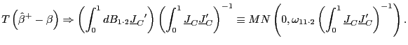
The corresponding test-statistics will now have standard distributions asymptotically. For instance, the
under the null, as
The ![]() statistic is identical to the
statistic is identical to the ![]() statistic of Campbell and Yogo
(2005). Whereas Campbell and Yogo (2005) attack the problem from a
test point-of-view, the derivation in this paper starts with the
estimation problem and delivers the test-statistic as an immediate
consequence. However, presenting the derivation in this manner
makes clear that this approach is a generalization of fully
modified estimation.
statistic of Campbell and Yogo
(2005). Whereas Campbell and Yogo (2005) attack the problem from a
test point-of-view, the derivation in this paper starts with the
estimation problem and delivers the test-statistic as an immediate
consequence. However, presenting the derivation in this manner
makes clear that this approach is a generalization of fully
modified estimation.
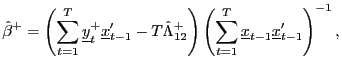
In addition, if Assumption 1 is replaced by the stronger
condition that both ![]() and
and ![]() are martingale
difference sequences, it is easy to show that OLS estimation of the
augmented regression
are martingale
difference sequences, it is easy to show that OLS estimation of the
augmented regression
yields an estimator of ![]() with an asymptotic distribution identical to
that of
with an asymptotic distribution identical to
that of
![]() . This
is, of course, a straightforward extension of the results in
Phillips (1991) for unit-root regressors. Moreover, in the
unit-root case, Phillips (1991) shows that the OLS estimator of
. This
is, of course, a straightforward extension of the results in
Phillips (1991) for unit-root regressors. Moreover, in the
unit-root case, Phillips (1991) shows that the OLS estimator of
![]() in equation (8)
is identical to the gaussian full system maximum likelihood
estimator of
in equation (8)
is identical to the gaussian full system maximum likelihood
estimator of ![]() . The
optimality properties of Campbell and Yogo's (2005)
. The
optimality properties of Campbell and Yogo's (2005) ![]() test is thus a direct extension of
the optimality results developed in Phillips (1991).
test is thus a direct extension of
the optimality results developed in Phillips (1991).
References
1. Campbell, J.Y., and M. Yogo, 2005. Efficient Tests of Stock Return Predictability, forthcoming Journal of Financial Economics.
2. Cavanagh, C., G. Ellliot, and J. Stock, 1995. Inference in models with nearly integrated regressors, Econometric Theory 11, 1131-1147.
3. Jansson, M., and M.J. Moreira, 2004. Optimal Inference in Regression Models with Nearly Integrated Regressors, NBER Working Paper T0303.
4. Lewellen, J., 2004. Predicting returns with financial ratios, Journal of Financial Economics, 74, 209-235.
5. Mankiw, N.G., and M.D. Shapiro, 1986. Do we reject too often? Small sample properties of tests of rational expectations models, Economic Letters 20, 139-145.
6. Phillips, P.C.B, 1987. Towards a Unified Asymptotic Theory of Autoregression, Biometrika 74, 535-547.
7. Phillips, P.C.B, 1988. Regression Theory for Near-Integrated Time Series, Econometrica 56, 1021-1043.
8. Phillips, P.C.B, 1991. Optimal Inference in Cointegrated Systems, Econometrica 59, 283-306.
9. Phillips, P.C.B, 1995. Fully Modified Least Squares and Vector Autoregression, Econometrica 63, 1023-1078.
10. Phillips, P.C.B, and B. Hansen, 1990. Statistical Inference in Instrumental Variables Regression with I(1) Processes, Review of Economic Studies 57, 99-125.
11. Stambaugh, R., 1999. Predictive regressions, Journal of
Financial Economics 54, 375-421.
Footnotes
1. Tel.: +1-202-452-2436; fax: +1-202-263-4850; email: [email protected]. The views presented in this paper are solely those of the author and do not represent those of the Federal Reserve Board or its staff. Return to text
2. The definition of
![]() is slightly different from the one found in Phillips (1995). This
is due to the predictive nature of the regression equation
(1), and the martingale difference sequence
assumption on
is slightly different from the one found in Phillips (1995). This
is due to the predictive nature of the regression equation
(1), and the martingale difference sequence
assumption on ![]() . Return to
text
. Return to
text
This version is optimized for use by screen readers. A printable pdf version is available.