Skip to: [Printable Version (PDF)]

Board of Governors of the Federal Reserve System
International Finance Discussion Papers
Number 871, September 2006-Screen Reader Version*

Real-Time Price Discovery in Global Stock, Bond and Foreign Exchange Markets

Torben G. Andersen, Tim Bollerslev, Francis X. Diebold, and Clara Vega^*

NOTE: International Finance Discussion Papers are preliminary materials circulated to stimulate discussion and critical comment. References in publications to International Finance Discussion Papers (other than an acknowledgment that the writer has had access to unpublished material) should be cleared with the author or authors. Recent IFDPs are available on the Web at http://www.federalreserve.gov/pubs/ifdp/. This paper can be downloaded without charge from the Social Science Research Network electronic library at http://www.ssrn.com/.

^*This work was supported by the National Science Foundation, the Guggenheim Foundation, and the BSI Gamma Foundation. For useful comments we thank the Editor and referees, seminar participants at the Bank for International Settlements, the BSI Gamma Foundation, the Symposium of the European Central Bank / Center for Financial Studies Research Network, the NBER International Finance and Macroeconomics program, and the American Economic Association Annual Meetings, as well as Rui Albuquerque, Annika Alexius, Boragan Aruoba, Anirvan Banerji, Ben Bernanke, Robert Connolly, Jeffrey Frankel, Lingfeng Li, Richard Lyons, Marco Pagano, Paolo Pasquariello, and Neng Wang. Andersen is affiliated with the department of finance, Northwestern University, and NBER, [email protected]. Bollerslev is affiliated with the departments of economics and finance, Duke University, and NBER, [email protected]. Diebold is affiliated with the departments of economics, finance and statistics, University of Pennsylvania, and NBER, [email protected]. Vega is affiliated with the Board of Governors of the Federal Reserve System and William E. Simon Graduate School of Business Administration, University of Rochester, [email protected]. Return to text

Abstract:

Using a unique high-frequency futures dataset, we characterize the response of U.S., German and British stock, bond and foreign exchange markets to real-time U.S. macroeconomic news. We find that news produces conditional mean jumps; hence high-frequency stock, bond and exchange rate dynamics are linked to fundamentals. Equity markets, moreover, react differently to news depending on the stage of the business cycle, which explains the low correlation between stock and bond returns when averaged over the cycle. Hence our results qualify earlier work suggesting that bond markets react most strongly to macroeconomic news; in particular, when conditioning on the state of the economy, the equity and foreign exchange markets appear equally responsive. Finally, we also document important contemporaneous links across all markets and countries, even after controlling for the effects of macroeconomic news.

Keywords: Asset Pricing; Macroeconomic News Announcements; Financial Market Linkages; Market Microstructure; High-Frequency Data; Survey Data; Asset Return Volatility; Forecasting.

JEL Classification: F3, F4, G1, C5

1  Introduction

How do markets arrive at prices? There is perhaps no question more central to economics. This paper focuses on price formation in financial markets, where the question looms large: How, if at all, is news about macroeconomic fundamentals incorporated in pricing stocks, bonds and foreign exchange?

Unfortunately, the process of price discovery in financial markets remains poorly understood. Traditional ``efficient markets'' thinking suggests that asset prices should completely and instantaneously reflect movements in underlying fundamentals. Conversely, others feel that asset prices and fundamentals may be largely and routinely disconnected. Experiences such as the late 1990s U.S. market bubble would seem to support that view, yet simultaneously it seems clear that financial market participants pay a great deal of attention to data on underlying economic fundamentals. The notable difficulty of empirically mapping the links between economic fundamentals and asset prices is indeed striking.

The central price-discovery question has many dimensions and nuances. How quickly, and with what patterns, do adjustments to news occur? Does announcement timing matter? Are the magnitudes of effects similar for ``good news'' and ``bad news,'' or, for example, do markets react more vigorously to bad news than to good news? Quite apart from the direct effect of news on assets prices, what is its effect on financial market volatility? Do the effects of news on prices and volatility vary across assets and countries, and what are the links? Are there readily identifiable herd behavior and/or contagion effects? Do news effects vary over the business cycle?

Just as the central question of price discovery has many dimensions and nuances, so too does a full answer. Appropriately then, dozens -- perhaps hundreds -- of empirical papers chip away at the price discovery question, but most fall short of our goals in one way or another. Some examine the connection between macroeconomic news announcements and subsequent movements in asset prices, but only for a single asset class and country (e.g., Balduzzi, Elton and Green, 2001, who study the U.S. bond market). Others examine multiple asset classes but only a single country (e.g., Boyd, Jagannathan and Hu, 2005, who study U.S. stock and bond markets). Still others examine multiple countries but only a single asset class (e.g., Andersen, Bollerselev, Diebold and Vega, ABDV 2003, who study several major U.S. dollar exchange rates).

Now, however, professional attention is turning toward multiple countries and asset classes.¹ Our paper is firmly in that tradition. We progress by studying a broad set of countries and asset classes, characterizing the joint response of foreign exchange markets as well as the domestic and foreign stock and bond markets to real-time U.S. macroeconomic news. We simultaneously combine: (1) high-quality and ultra-high frequency asset price data across markets and countries, which allows us to study price movements in (near) continuous time; (2) a very broad set of synchronized survey data on market participants' expectations, which allow us to infer ``surprises'' or ``innovations'' when news is announced; and (3) advances in statistical modeling of volatility, which facilitate efficient inference.

We proceed in straightforward fashion: In section 2 we describe our data. In section 3 we present our basic results, and in section 4 we present results obtained using a generalized model specification. We conclude in section 5.

2  High-Frequency Return Data

Here we discuss our return data. We begin by describing its sources and construction, and then we examine its features, stressing various correlations during news announcement times, ultimately allowing for different correlation structures in expansions vs. contractions.

Futures Market Return Data

We use futures market data for several reasons. First, futures prices are readily available on a tick-by-tick basis. Second, most significant U.S. macroeconomic news announcements are released at 8:30 Eastern Standard Time (EST) when the futures markets are open, but the equity markets closed. Third, transaction costs are lower in the futures markets, and the contracts we analyze are very actively traded. Indeed, numerous studies find that futures markets tend to lead cash markets in terms of price discovery.² This is important, as we focus on price adjustments measured over very short time intervals.

Table 1 provides an overview of the specific contracts, the exchanges on which they trade, and their trading hours, along with the average number of contracts traded daily. The S&P500, $/Pound, $/Yen and $/Euro futures contracts are listed on the Chicago Mercantile Exchange (CME).³ Trading in the foreign exchange contracts starts at 8:20 EST, while the regular trading hours for S&P500 are 9:30 to 16:15 EST. However, beginning January 2, 1994, GLOBEX offered automated pre-market trading in the S&P500 futures contract, so we use the GLOBEX transactions data to start the S&P500 trading day at 8:20 EST. Our data for the 30-Year U.S. Treasury Bond futures contract comes from the Chicago Board of Trade (CBOT) whose trading hours coincide with those of the CME. The FTSE 100 and the British Long Gilt futures contracts trade on the London International Financial Futures Exchange (LIFFE). The FTSE 100 index is based on the one-hundred largest U.K. companies, while the Long Gilt contract is based on the British 10-Year Treasury note. Trading on LIFFE opens at 8:00 GMT, or 3:00 EST. Both of our last two contracts, the DJ Euro Stoxx 50 (DJE) and the Euro Bobl futures, trade on the European Exchange (EUREX). The DJE index is composed of the fifty largest blue-chip market sector leaders in the Euro-zone countries. The Euro Bobl is based on the German 5-Year Treasury note.

We obtained raw tick-by-tick transaction prices for all contracts from Tick Data Inc. The sample for the foreign exchange rates and the U.S. Treasury Bond contracts spans January 2, 1992 through December 31, 2002. Because of the need for pre-market GLOBEX data to augment the trading day, our sample for the S&P500 starts two years later on January 2, 1994. Data on the four European contracts are only available from July 1, 1998 through December 31, 2002.

All results reported below are based on five-minute local currency continuously compounded returns, $\log( \mathop p\nolimits_{t} / \mathop p\nolimits_{t-1} )$, where $\mathop p\nolimits_{t}$ denotes the price of the last trade in the $t$'th five-minute interval.⁴ If no trade occurs in a given five-minute interval, we use the price from the previous interval, as long as the previous price was quoted within the last half-hour. We include only the days where there were at least one trade every half-hour. We always use the most actively traded nearest-to-maturity contract, switching to the next-maturity contract five days before expiration.

High-Frequency Returns around Macroeconomic News Announcements

Table 2 reports summary statistics for the five-minute return series around the announcement times. Since our news announcement regressions are based on the period ranging from ten minutes before to one-and-a-half hours after an announcement, we let the sample cover this set of returns only. Moreover, to provide a meaningful benchmark for the subsequent results based on simultaneous estimation across all the markets, we further restrict the sample for all contracts to July 1, 1998 to December 31, 2002, the period available for the shortest series, namely the European markets.

The average five-minute return for each of the nine markets is, as expected, extremely close to zero. However, the (absolute) size of the largest five-minute returns is noteworthy, with the extreme return event being about ten standard deviations or more removed from the sample mean for all markets. For the S&P500 and the DJE these extreme moves exceed two percent. This immediately suggests that macroeconomic news does move the markets.⁵ The summary statistics confirm the usual rank ordering in terms of volatility, with stock markets being the most volatile, followed by foreign exchange rates, and then fixed income. The only exception to this rule is the U.S. T-Bond market, for which the unconditional return standard deviation actually exceeds the standard deviations for the three exchange rates. This is likely a consequence of the fact that the T-Bond market, as discussed further below, reacts most strongly to macroeconomic news.

To provide a sense of the comovements among the asset markets during news announcement times, Table 3 reports unconditional sample correlations. All correlations within each of the three asset classes are positive. For instance, the stock market correlations range from a low of 0.42 between the S&P500 and the FTSE 100, to a high of 0.54 for the FTSE 100 and the DJE. Similarly, the correlation between the returns for the U.S. T-Bond and the British Long Gilt is 0.53, while the Gilt and German Euro Bobl correlation is 0.61. The positive bond market cross-correlations during U.S. macroeconomic news announcement times match standard theoretical predictions, such as those of Lucas (1982).⁶ The positive equity market cross-correlations are similarly consistent with the Lucas model, although they are not directly implied by it as three separate influences determine the equity prices: the risk-free interest rate, expected future cash flows and the equity risk premium. Stock market prices around the world would tend to be positively correlated if the discount rate is the dominant effect or if the domestic and foreign real output and/or monetary shocks are positively correlated.⁷

The cross correlations between the different asset types are generally much smaller than the cross correlations within the same asset category across countries. Given our American exchange rate quotation convention ($/Euro, $/Pound, $/yen), the negative correlations between the S&P500 and the exchange rates imply that U.S. macroeconomic news affects the Dollar and the equity market in the same direction. Interestingly, a Dollar appreciation also is associated with stock market increases abroad, even though one may expect the Dollar to depreciate against the Pound (Euro) when the FTSE 100 (DJE) prices are rising. This again suggests that the U.S. macroeconomic fundamentals exert a dominant effect during the news announcement period. It also serves as a warning that it may be important to control explicitly for macroeconomic fundamentals when interpreting asset market correlations. Subsequently we attempt to do so in a simultaneous equations setting.

Correlations in Expansions vs. Contractions

It is interesting to ask whether the interactions among asset returns and their responses to macroeconomic fundamentals vary systematically across the business cycle. For a preliminary look at this issue, the bottom panels in Table 3 report the unconditional correlations separately for the expansion period from July 1998 through February 2001 and the contraction period from March 2001 through December 2002.⁸ During the expansion, the stock-bond correlations are positive albeit small, whereas during the contraction they are negative and large. We cannot claim this as a general pattern, as we only have data for one expansion and one contraction. Still, one possible explanation is that the cash flow effect dominates during contractions while the discount effect dominates in expansions (due to central bank policy), producing positive stock-bond return correlations during expansions and negative in contractions, in confirmation of the seminal contribution of Boyd, Jagannathan and Hu (2005). In what follows, we explore that possibility in depth.

3  Asset Returns and Macroeconomic Surprises: Basic Results

Here we characterize the dynamic effects of U.S. macroeconomic news announcements for each of our nine asset markets. We begin by describing our measurement of macroeconomic news, and then we estimate responses of asset returns to news, both over the full sample and separately for expansions and contractions.

Macroeconomic News

We use the International Money Market Services (MMS) real-time data on expected and realized U.S. macroeconomic fundamentals, defining ``news'' as the difference between the survey expectations and the subsequently announced realizations. The MMS sample covers the period from January 1, 1992 through December 31, 2002. Table 4 provides a basic description of the announcement releases, including the number of observations, the agency reporting the news, and the time of the release.⁹

The units of measurement obviously differ across the macroeconomic indicators. Hence, to allow for meaningful comparisons of the estimated news response coefficients across indicators and asset classes, we follow Balduzzi, Elton and Green (2001) and ABDV (2003) in the use of ``standardized news.'' Specifically, we divide the surprise by its sample standard deviation, defining the standardized news associated with indicator $k$ at time $t$ as $\mathop S\nolimits_{kt} = (\mathop A\nolimits_{kt} -\mathop E\nolimits_{kt} ) / \mathop {\hat {\sigma }}\nolimits_{k} ,$ where $\mathop A\nolimits_{kt}$ denotes the announced value of indicator $k$, $\mathop E\nolimits_{kt}$ refers to the market's expectation of indicator $k$ as distilled in the MMS median forecast, and $\mathop {\hat {\sigma }}\nolimits_{k}$ is equal to the sample standard deviation of the surprise component, $\mathop A\nolimits_{kt} -\mathop E\nolimits_{kt}$. Because $\mathop {\hat {\sigma }}\nolimits_{k}$ is constant for any indicator $k$, this standardization affects neither the statistical significance of the estimated response coefficients nor the fit of the regressions compared to the results based on the ``raw'' surprises.

Dynamic News Effects

In order to analyze dynamic news effects, we estimate response equations using the two five-minute returns directly preceding and the eighteen five-minute returns following each announcement.¹⁰ To allow explicitly for cross-market linkages and dynamic responses to news, we model the conditional mean of the five-minute return for asset $h$, $\mathop R\nolimits_{t}^{h}$, as a linear function of $I$ lags of all returns, together with $J$ lags of each of the $K$ news announcements. (There are $H=9$ different assets.) Specifically,

$$\mathop R\nolimits_{t}^{h}=\mathop\beta\nolimits_{0}^{h}+\mathop\sum \limits_{{h}^{\prime}=1}^{H}\mathop\sum\limits_{i=1}^{I}\mathop\beta \nolimits_{hi}^{{h}^{\prime}}\mathop R\nolimits_{t-i}^{{h}^{\prime} }+\mathop\sum\limits_{k=1}^{K}\mathop\sum\limits_{j=0}^{J}\mathop\beta \nolimits_{kj}^{h}\mathop S\nolimits_{k,t-j}+\mathop\varepsilon\nolimits_{t} ^{h},t=1,...,T,$$ (3.1)

where $\mathop R\nolimits_{t}^{h}=\log(\mathop p\nolimits_{t}^{h} /\mathop p\nolimits_{t-1}^{h})$ denotes the five-minute futures return corresponding to asset $h$ ($h$ = $/BP, $/Yen, $/Euro, S&P500, T-Bond, Gilt, Bobl, FTSE, and DJE) from time $t$ to time $t+1$, $\mathop S\nolimits_{kt}$ refers to the standardized news for indicator $k$ ( $k=1,...,25)$ at time $t$, and the estimates are based on only those observations ( $\mathop R\nolimits_{t}^{h},\mathop S\nolimits_{kt})$ where an announcement was made at time $t$.

Because the consumer credit, government budget, and federal funds rate figures are released in the afternoon, when LIFFE and EUREX are closed, we have a total of$K=22$ indicators. Guided by the Schwarz and Akaike information criteria, we uniformly fix the two lag lengths at $I=2$ and $J=3$, resulting in a total of 107 regression coefficients to be estimated for each of the nine assets.

We perform both full-sample regressions and split-sample regressions (expansion / contraction, with the full sample July 1, 1998 through December 31, 2002, and the expansion and contraction periods based on the observations before and after February 28, 2001, respectively. This leaves us with a full sample of T = 15,764 = 544x20 + 40x29 + 98x38 five-minute return observations, reflecting 544 days with only one macroeconomic announcement released on that day (20 observations per day), 40 days with two announcements, one at 8:30 EST and the other one at 9:15 EST (29 observations per day), and 98 days with two announcements, one at 8:30 EST and the other at 10:00 EST (38 observations per day). The expansion sample is comprised of the first 9,301 observations, while the last 6,463 observations constitute the contraction sample.

Although ordinary least squares (OLS) would be consistent for the parameters in (3.1), the disturbance terms for the five-minute return regressions are clearly heteroskedastic. Thus, to enhance the efficiency of the coefficient estimates, we use a two-step weighted least squares (WLS) procedure. We first estimate the conditional mean model by OLS. We then use the absolute value of the regression residuals, $\vert\mathop {\hat {\varepsilon }}\nolimits_{t}^{h}\vert$, to estimate a time-varying volatility function, which we then subsequently use to perform weighted least squares estimation of (3.1). We approximate the temporal variation in the five-minute return volatility around the announcement times by the relatively simple regression model,

$$\vert\mathop {\hat {\varepsilon }}\nolimits_{t}^{h}\vert=\mathop\sum\limits_{i=1} ^{{I}^{\prime}}\mathop\beta\nolimits_{hi} \vert\mathop {\hat {\varepsilon }}\nolimits_{t-i}^{h}\vert+\mathop\sum\limits_{d=1} ^{D}\mathop\gamma\nolimits_{d}\mathop D\nolimits_{d}+\mathop\sum \limits_{k=1}^{\mathop K\nolimits_{d}}\mathop\sum\limits_{{j}^{\prime}=0} ^{{J}^{\prime}}\mathop\gamma\nolimits_{{k}^{\prime}j}^{h} \mathop D\nolimits_{k,t-{j}^{\prime}}+\mathop u\nolimits_{t}^{h}.$$ (3.2)

The ${I}^{\prime}=9$ own lags of the absolute value of the residuals captures serial correlation, or ARCH effects. The next term involves $D=38$ dummy variables for each of the five-minute intraday intervals. This term directly accounts for the well-documented intradaily volatility patterns; see, e.g., the discussion and references in Andersen and Bollerslev (1998). The last summation reflects dummy variables for each of the announcement surprises, $\mathop D\nolimits_{k,t}$, up to a lag length of ${J}^{\prime}=14$. There are only $\mathop K\nolimits_{d}=20$ such dummies as capacity utilization and industrial production, and personal consumption expenditures and personal income, are announced at the same time.¹¹

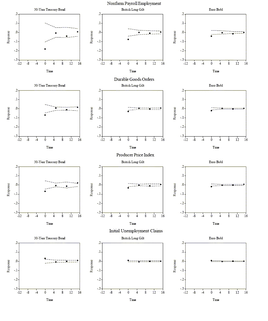
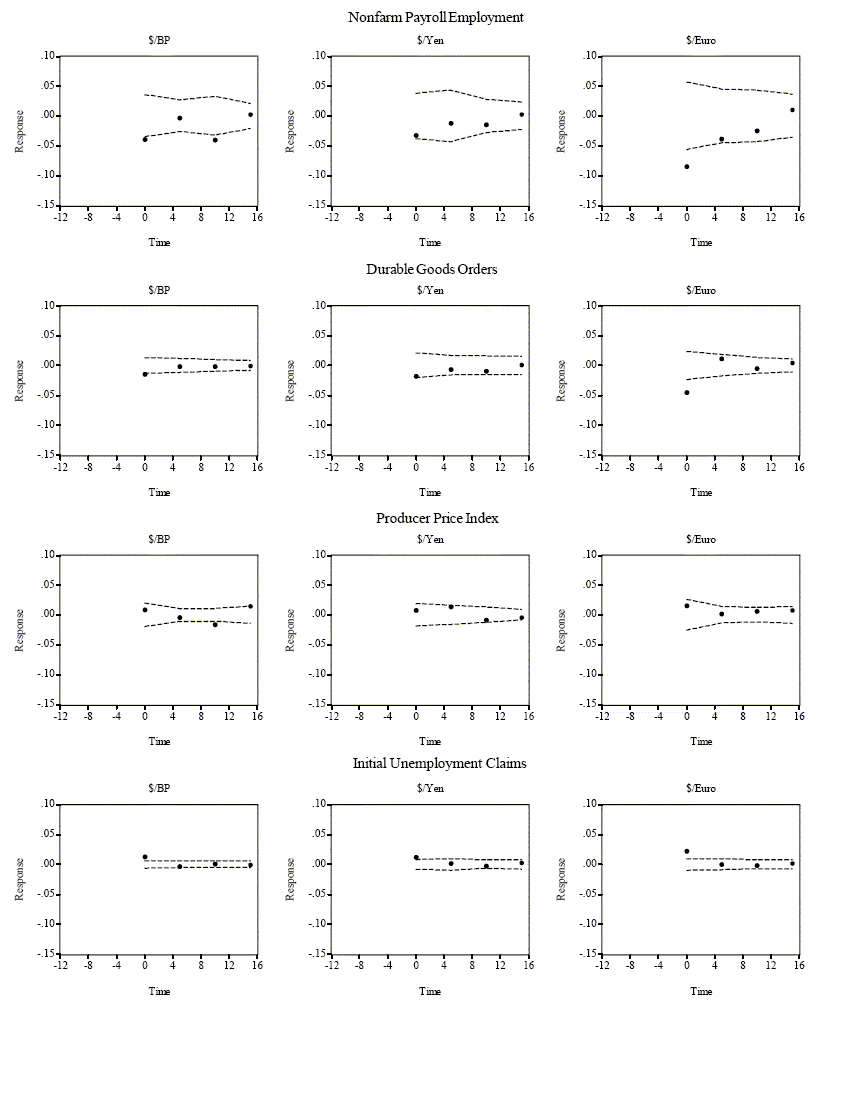
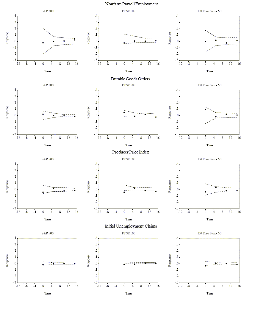
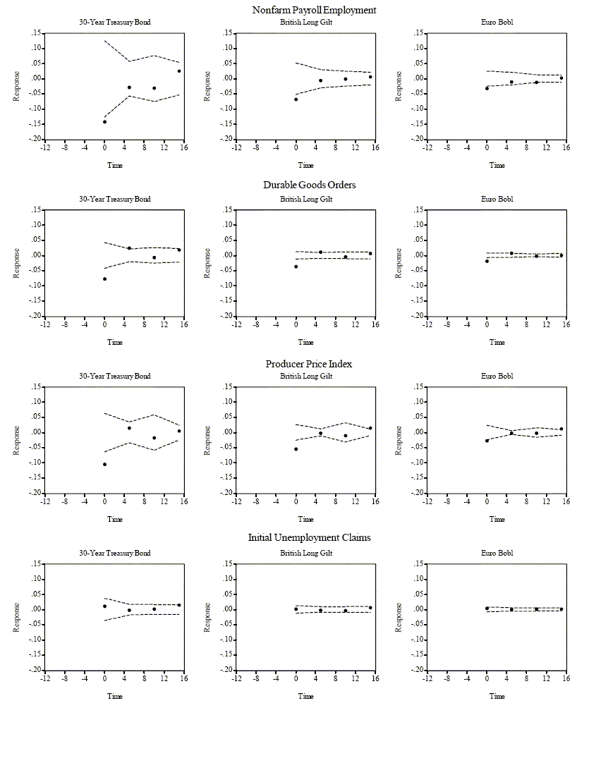
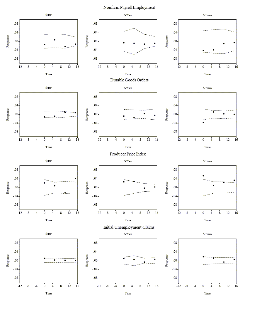
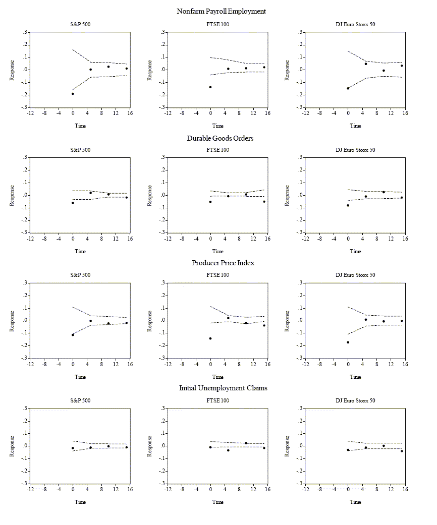
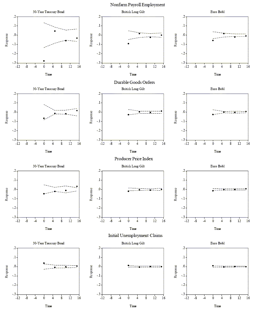
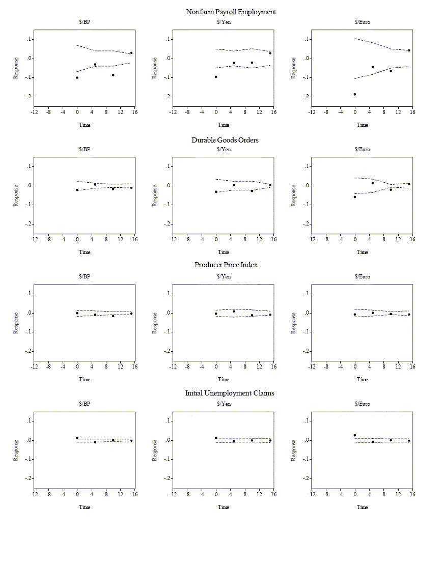
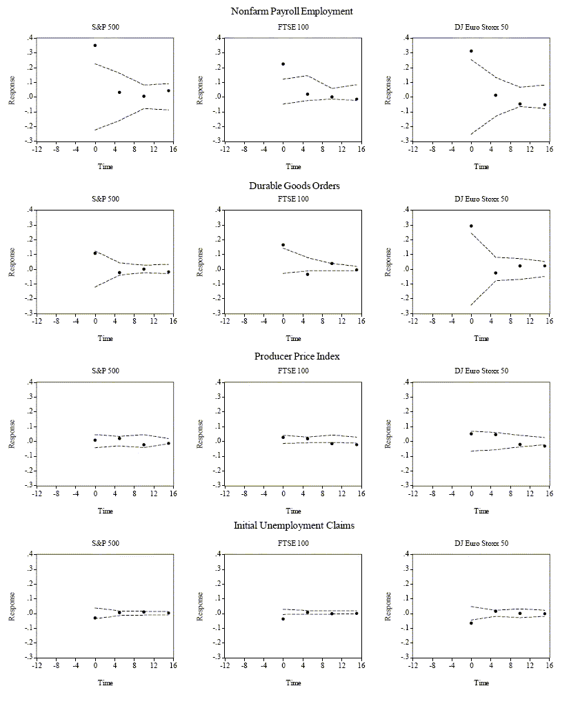
Because the model in (3.1) contains so many variables and lags, it is counterproductive to report all the parameter estimates.¹² Instead, in Figures 1A-1C, we present graphically the point estimates for the news response coefficients, $\mathop \beta \nolimits_{kj}^{h} , j = 0, ... , 3$, for some key indicators at the time of the news releases and fifteen-minutes thereafter (dots), along with corresponding robust ninety-percent confidence bands (dashes). Figure 1A covers the full sample, while the results for the expansion and contraction periods appear in Figures 1B and 1C. All figures contain three panels; the first displays the news responses for the domestic and foreign bond markets, the second focuses on the foreign exchange markets, and the last reports the results for the domestic and foreign equity markets.

Consider first the bond market responses. The immediate reactions are qualitatively similar to those discussed earlier for the U.S. T-bond market over the longer eleven-year sample. Regardless of the stage of the business cycle, positive real shocks and inflationary shocks produce lower bond prices, or higher yields. Not surprisingly, the effects are clearly the strongest in the U.S., but many of the U.S. macroeconomic fundamentals also significantly impact the foreign bond markets, and in the same direction. This is, of course, consistent with basic theoretical predictions. It is noteworthy that, almost invariably, only the simultaneous effect is significant, reflecting a very quick price discovery process.

The near instantaneous response holds true for all markets. Any systematic effect is almost exclusively restricted to the five-minute interval following the news release. This helps explain why previous studies relying on daily, or coarser, observations typically have failed to uncover systematic links between asset market returns and innovations to macroeconomic fundamentals -- the responses occur almost instantaneously and tend to ``drown'' in the overall day-to-day price movements. Hence, the only way to assess the connection between the news releases and the asset prices with some degree of precision is to focus on the high-frequency returns just around the announcement time.

The findings for the equity markets are striking. The full-sample results in Figure 1A reveal almost no significant responses, but once we split the sample into the expansion and contraction periods, we see that positive real economic shocks are met with a negative response in expansions and a positive response in contractions. As discussed previously, this pattern, which is identical for the domestic and foreign markets, is suggestive of positively correlated real economic shocks across the regions along with pronounced business cycle variation in the importance of the discount factor versus cash flow components in the markets' valuation of equities. This is further corroborated by the asymmetric effect of the PPI shocks over the business cycle. The marked negative impact of inflation surprises during expansions suggests the presence of stronger anti-inflationary monetary policies, in turn strengthening the influence of the discount factor component in ``good'' economic times.

Finally, turning to the foreign exchange markets, news about the U.S. inflation rate does not seem to systematically affect the foreign exchange rates, while positive domestic real shocks lead to an appreciation of the Dollar, particularly during the recent contraction regime.

A Closer Look at Stock-Bond Correlations

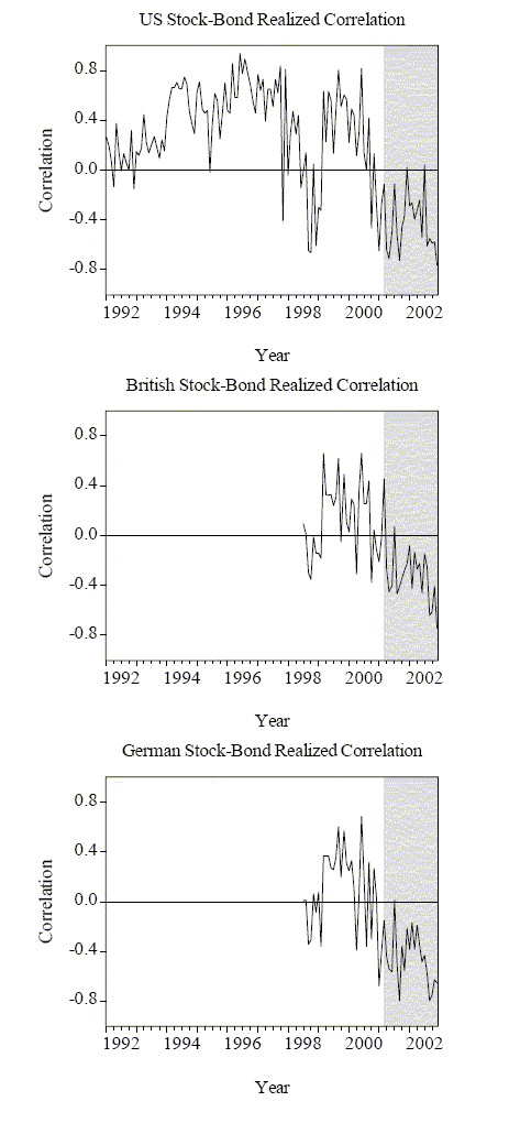
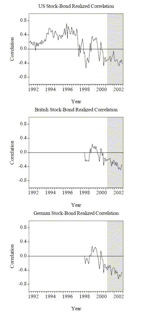
The apparent state dependence in the equity markets news reaction function coupled with the time-invariant reaction of the bond markets naturally translates into state dependent stock-bond market correlations, with price changes being positively correlated during expansions and negatively correlated during contractions. Indeed, the unconditional sample correlations for the expansion and contraction periods discussed in Table 3 already point to the existence of time-varying cross-market dependence. In order to explore this effect in more detail, we display in Figure 2A the daily realized correlations in each country computed from the high-frequency stock-bond market returns for the days containing the arguably most important U.S. macroeconomic announcement, namely the nonfarm payroll employment release.¹³ Figure 2B depicts the corresponding realized correlations over the entire month, which aids assessment of whether the correlation patterns are driven by the macroeconomic news releases or whether they simply indicate the general relationship among the markets. The computations follow the methodology described in Andersen, Bollerslev, Diebold and Labys (2001, 2003). To facilitate cross country comparisons, we restrict the calculations to encompass the common trading hours from 8:20 to 12:30 EST, resulting in a total of 51 5-minute intervals per day and approximately 51x22 = 1,122 5-minute observations per month. Specifically, we define

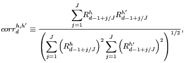
$$corr_{d}^{h,h^{\prime}}\equiv\frac{ {\displaystyle\sum\limits_{j=1}^{J}} R_{d-1+j/J}^{h}R_{d-1+j/J}^{h^{\prime}}}{\left( {\displaystyle\sum\limits_{j=1}^{J}} \left( R_{d-1+j/J}^{h}\right) ^{2} {\displaystyle\sum\limits_{j=1}^{J}} \left( R_{d-1+j/J}^{h^{\prime}}\right) ^{2}\right) ^{1/2}},$$ (3.3)

where $J=51$ ( $J\approx1122)$ for the daily (monthly) correlations, and $d$ refers to the corresponding daily (monthly) index.¹⁴

Turning to the two figures, the time varying stock-bond correlations are remarkably similar across countries, not only for the nonfarm payroll announcement dates (Figure 2A), but also when calculated for the full month (Figure 2B). The correlations are generally higher and mostly positive during the expansion period and smaller and negative during the contraction period. Interestingly, there is also an indication that the correlations may evolve smoothly, shifting rather slowly from values typical of expansion to those typical of contraction. Moreover, there is a noticeable drop just around August and September of 1998, which corresponds to the Russian debt default crises and the Long Term Capital Management (LTCM) hedge fund collapse, at which time the Federal Reserve actively intervened to avoid spillovers into the global capital markets. This episode is well known to have increased credit spreads on risky securities worldwide. The burst of uncertainty regarding the financial and economic health of the international economy is clearly reflected in our correlation measures as they take on a pattern otherwise only observed during the contraction. Our European series are somewhat contaminated by this event as they only are observed from July, 1998 onward. Ignoring the immediate aftermath of the financial crisis in late 1998, the switch in the sign of the correlations matches almost perfectly the previously exogenously imposed U.S. business cycle regime.

Our analysis is, of course, limited to the relatively short calendar time span and single U.S. expansion-contraction period covered by the high-frequency data.¹⁵ Nonetheless, it is noteworthy that even though the German and British's business cycles do not necessarily coincide with the U.S. business cycle, it appears as though the relevant state variable for determining the time-varying impact of the news announcements is the state of the U.S. economy rather than the foreign country.¹⁶ Indeed, the patterns in the time-varying correlations are entirely consistent with our previous assertion that the discount rate effect dominates in each of the three stock markets during U.S. economic expansions, coupled with the U.S. interest rate playing the role of the ``world interest rate'' and hence dictating the move of the foreign bond markets.¹⁷

4  A Generalized Specification

We have argued that the movements in asset returns across markets and countries documented above are driven by the common exposure to exogenous U.S. macroeconomic shocks and the U.S. business cycle. This contrasts with previous studies that also document important spillover effects and market linkages, but little (if any) role for macroeconomic fundamentals in explaining the comovements between markets. Our positive results can be attributed to our focus on synchronous high-frequency data around the time of the announcement -- all assets are actively traded during announcement times, so we observe the immediate news reaction of all assets -- which mitigates other influences and potentially important omitted variables biases.

To further investigate the extent of the cross-market and cross-country links in the high-frequency data, beyond the direct influence of the macroeconomic news announcement effects, it is informative to consider the simultaneous equations model,

$$\mathop R\nolimits_{t}^{h}=\mathop\beta\nolimits_{0}^{h}+\mathop\sum \limits_{{h}^{\prime}\neq h}\mathop\beta\nolimits_{h0}^{{h}^{\prime} }\mathop R\nolimits_{t}^{{h}^{\prime}}+\mathop\sum\limits_{{h}^{\prime}=1} ^{H}\mathop\sum\limits_{i=1}^{I}\mathop\beta\nolimits_{hi}^{{h}^{\prime} }\mathop R\nolimits_{t-i}^{{h}^{\prime}}+\mathop\sum\limits_{k=1} ^{K}\mathop\sum\limits_{j=0}^{J}\mathop\beta\nolimits_{kj}^{h} \mathop S\nolimits_{k,t-j}+\mathop\eta\nolimits_{t}^{h} ,\;\;\;\;t=1,...,T.$$ (4.1)

Except for the inclusion of the contemporaneous asset returns on the right-hand side, the model is identical to our basic model (3.1). As in equation (3.1), the $\mathop\beta\nolimits_{k0}^{h}$ coefficients directly capture the U.S. macroeconomic announcement effects, while the $\mathop\beta \nolimits_{h0}^{{h}^{\prime}}$ account for any contemporaneous cross-asset linkages and/or spillover effects that are not explained by the news announcements. This could include reaction to other fundamental information as well as non-fundamental market microstructure, contagion, and cross-hedging effects. The problem from an econometric perspective is that, without any additional restrictions or modeling assumptions, the contemporaneous coefficients in $\mathop\beta \nolimits_{h0}^{{h}^{\prime}}$ are not identified.

To overcome this problem, we follow the approach of a recent series of papers by Rigobon (2003), Rigobon and Sack (2003a,b, 2004), and Sentana and Fiorentini (2001), who use the conditional heteroskedasticity in the high-frequency data to identify the contemporaneous response coefficients. The idea is straightforward. Assuming that the innovations in (4.1) are conditionally uncorrelated but heteroskedastic -- as indicated by our previous estimation results for (3.2) -- the conditional covariances of the implied (3.1) innovations will then move in proportion to the conditional heteroskedasticity in the (4.1) innovations, with the factors of proportionality determined by $\mathop\beta \nolimits_{h0}^{{h}^{\prime}}$. This proportionality in turn, allows for the identification and estimation of the contemporaneous response coefficients.¹⁸

Our approach follows Rigobon and Sack (2003b), in estimating the elements of $\mathop\beta \nolimits_{h0}^{{h}^{\prime}}$ by applying Gaussian quasi-maximum likelihood estimation (QMLE) techniques to the multivariate GARCH model implied by univariate GARCH models for each of the individual equations in (4.1).¹⁹ To facilitate the implementation of the multivariate GARCH model, we treat the residuals from the first-stage estimation of (3.1) as directly observable. Also, for tractability, we estimate the model for three markets at a time, but the same idea could in principle be applied to any number of assets.

Focusing first on the trivariate domestic system consisting of U.S. T-Bond, S&P500, and $/Euro returns, we obtain the following estimates for the contemporaneous linkages among the three markets based on the 9,301 five-minute announcement period returns spanning the July 1, 1998 through February 28, 2001 expansion time period:

$${\begin{array}{*{20}c} {\mathop R\nolimits_t^{TBond} } & { = - 0.026 \mathop R\nolimits_t^{S\& P} } & {+ 0.020 \mathop R\nolimits_t^{\$ /Euro} } & {+ \mathop \beta \nolimits_0^h + \mathop \sum \limits_{{h}'=1}^H \mathop \sum \limits_{i=1}^I \mathop \beta \nolimits_{hi}^{{h}'} \mathop R\nolimits_{t-i}^{{h}'} + \mathop \sum \limits_{k=1}^K \mathop \sum \limits_{j=0}^J \mathop \beta \nolimits_{kj}^h \mathop S\nolimits_{k,t-j} + \mathop \eta \nolimits_t^h } \\ { } & { (-9.41)} & {(3.34)} & { } \\ \end{array}}$$ (4.2)

$${\begin{array}{*{20}c} {\mathop R\nolimits_t^{S\& P} } & { = 0.204 \mathop R\nolimits_t^{TBond} } & {+ 0.120 \mathop R\nolimits_t^{\$ /Euro} } & {+ \mathop \beta \nolimits_0^h + \mathop \sum \limits_{{h}'=1}^H \sum \limits_{i=1}^I \mathop \beta \nolimits_{hi}^{{h}'} \mathop R\nolimits_{t-i}^{{h}'} + \mathop \sum \limits_{k=1}^K \mathop \sum \limits_{j=0}^J \mathop \beta \nolimits_{kj}^h \mathop S\nolimits_{k,t-j} + \mathop \eta \nolimits_t^h } \\ { } & {(25.33)} & {(14.88)} & { } \\ \end{array}}$$ (4.3)

$${\begin{array}{*{20}c} {\mathop R\nolimits_t^{\$ /Euro} } & { = 0.030 \mathop R\nolimits_t^{TBond} } & { - 0.002 \mathop R\nolimits_t^{S\& P} } & {+ \mathop \beta \nolimits_0^h + \mathop \sum \limits_{{h}'=1}^H \sum \limits_{i=1}^I \mathop \beta \nolimits_{hi}^{{h}'} \mathop R\nolimits_{t-i}^{{h}'} + \mathop \sum \limits_{k=1}^K \mathop \sum \limits_{j=0}^J \mathop \beta \nolimits_{kj}^h \mathop S\nolimits_{k,t-j} + \mathop \eta \nolimits_t^h ,} \\ { } & {(12.53)} & {(-2.39)} & { } \\ \end{array}}$$ (4.4)

where the numbers in parentheses refer to robust t-statistics.²⁰ A number of the coefficients are highly significant and they all have a natural interpretation. For example, an increase in stock prices may be seen as a signal of a positive real activity or inflationary shock and the point estimate for the S&P500 return coefficient in (4.2) is entirely consistent with the implications of the stylized monetary model. The impact of the exchange rate returns is clearly less important, but the sign is compatible with exchange rate changes on balance reflecting real economic shocks. Equation (4.3) is also directly in line with our aforementioned discussion of the dominance of the ``discount'' factor component in the evaluation of stock prices during economic expansions, whereby higher bond prices (lower discount rates) are good for the stock market in good times. Similarly, dollar depreciation (interpreted as a negative real activity or deflationary shock) results in higher stock prices. Notice also that while the unconditional correlation between bond and stock prices for the expansion period reported in Table 3 is positive, the estimation method underlying equations (4.2)-(4.4) allows us to disentangle two opposing effects: bond prices affect stock prices positively, but stock prices affect bond prices negatively.²¹ Finally, interpreting negative bond returns and positive stock returns as indicators of real economic strength the associated appreciation of the Dollar implied by equation (4.4) is as expected.

Estimating the same set of equations for the 6,463 five-minute announcement period returns over the March 1, 2001 through December 31, 2002 contraction time period produces the following results:

$${\begin{array}{*{20}c} {\mathop R\nolimits_t^{TBond} } & { = -0.033 \mathop R\nolimits_t^{S\& P} } & {+ 0.010 \mathop R\nolimits_t^{\$ /Euro} } & {+ \mathop \beta \nolimits_0^h + \mathop \sum \limits_{{h}'=1}^H \sum \limits_{i=1}^I \mathop \beta \nolimits_{hi}^{{h}'} \mathop R\nolimits_{t-i}^{{h}'} + \mathop \sum \limits_{k=1}^K \mathop \sum \limits_{j=0}^J \mathop \beta \nolimits_{kj}^h \mathop S\nolimits_{k,t-j} + \eta_t^h } \\ { } & {(-6.26)} & {(0.47)} & { } \\ \end{array}}$$ (4.5)

$${\begin{array}{*{20}c} {\mathop R\nolimits_t^{S\& P} } & { = -0.192 \mathop R\nolimits_t^{TBond} } & {- 0.090 \mathop R\nolimits_t^{\$ /Euro} } & {+ \mathop \beta \nolimits_0^h + \mathop \sum \limits_{{h}'=1}^H \sum \limits_{i=1}^I \mathop \beta \nolimits_{hi}^{{h}'} \mathop R\nolimits_{t-i}^{{h}'} + \mathop \sum \limits_{k=1}^K \mathop \sum \limits_{j=0}^J \mathop \beta \nolimits_{kj}^h \mathop S\nolimits_{k,t-j} + \mathop \eta \nolimits_t^h } \\ { } & { (-3.88)} & {(-1.97)} & { } \\ \end{array}}$$ (4.6)

$${\begin{array}{*{20}c} {\mathop R\nolimits_t^{\$ /Euro} } & { = 0.033 \mathop R\nolimits_t^{TBond} } & { - 0.011 \mathop R\nolimits_t^{S\& P} } & {+ \mathop \beta \nolimits_0^h + \mathop \sum \limits_{{h}'=1}^H \sum \limits_{i=1}^I \mathop \beta \nolimits_{hi}^{{h}'} \mathop R\nolimits_{t-i}^{{h}'} + \mathop \sum \limits_{k=1}^K \mathop \sum \limits_{j=0}^J \mathop \beta \nolimits_{kj}^h \mathop S\nolimits_{k,t-j} + \eta_t^h .} \\ { } & {(2.70)} & {(-4.28)} & { } \\ \end{array}}$$ (4.7)

The estimates for equations (4.5) and (4.7) are qualitatively as before, although the linkages among the interest rate and the other variables appear to have declined. This is consistent with the interest rates being less sensitive to economic shocks during the contraction. In contrast, the difference in the estimates for the S&P500 returns in equations (4.3) and (4.6) is striking. The contemporaneous linkages between the stock market and the other markets flips sign between the two periods. As before, ``good news'' during expansions is ``bad news'' for stocks, but ``good news'' during contractions is good for the stock market. In summary, the dominant finding is that positive stock returns (positive real or inflationary shocks), ceteris paribus, always raise interest rates, while positive innovations to interest rates (real or inflationary shocks) have a strongly regime-dependent impact on stock returns, once again confirming the differential impacts of the cash-flow and the discount rate effects over the business cycle.

Finally, we use the same approach to estimate the interdependence among the national stock markets beyond the linkages explained by the U.S. macroeconomic announcements. As before, dividing the sample in two, we find for the expansion sample:

$${\begin{array}{*{20}c} {\mathop R\nolimits_t^{S\& P} } & { = 0.028 \mathop R\nolimits_t^{FTSE} } & {+ 0.007 \mathop R\nolimits_t^{DJE} } & {+ \mathop \beta \nolimits_0^h + \mathop \sum \limits_{{h}'=1}^H \mathop \sum \limits_{i=1}^I \mathop \beta \nolimits_{hi}^{{h}'} \mathop R\nolimits_{t-i}^{{h}'} + \mathop \sum \limits_{k=1}^K \mathop \sum \limits_{j=0}^J \mathop \beta \nolimits_{kj}^h \mathop S\nolimits_{k,t-j} + \mathop \eta \nolimits_t^h } \\ { } & { (5.83)} & {(2.00)} & { } \\ \end{array}}$$ (4.8)

$${\begin{array}{*{20}c} {\mathop R\nolimits_t^{FTSE} } & { = 0.014 \mathop R\nolimits_t^{S\& P} } & {+ 0.015 \mathop R\nolimits_t^{DJE} } & {+ \mathop \beta \nolimits_0^h + \mathop \sum \limits_{{h}'=1}^H \mathop \sum \limits_{i=1}^I \mathop \beta \nolimits_{hi}^{{h}'} \mathop R\nolimits_{t-i}^{{h}'} + \mathop \sum \limits_{k=1}^K \mathop \sum \limits_{j=0}^J \mathop \beta \nolimits_{kj}^h \mathop S\nolimits_{k,t-j} + \mathop \eta \nolimits_t^h } \\ { } & {(2.73)} & {(9.57)} & { } \\ \end{array}}$$ (4.9)

$${\begin{array}{*{20}c} {\mathop R\nolimits_t^{DJE} } & { = 0.089 \mathop R\nolimits_t^{S\& P} } & { + 0.001 \mathop R\nolimits_t^{FTSE} } & {+ \mathop \beta \nolimits_0^h + \mathop \sum \limits_{{h}'=1}^H \mathop \sum \limits_{i=1}^I \mathop \beta \nolimits_{hi}^{{h}'} \mathop R\nolimits_{t-i}^{{h}'} + \mathop \sum \limits_{k=1}^K \mathop \sum \limits_{j=0}^J \mathop \beta \nolimits_{kj}^h \mathop S\nolimits_{k,t-j} + \mathop \eta \nolimits_t^h .} \\ { } & { (13.26)} & {(0.23)} & { } \\ \end{array}}$$ (4.10)

Not surprisingly, all estimated coefficients are positive, indicating important cross-country linkages over-and-above those explained by the U.S. macroeconomic news releases. It is unclear whether these high-frequency international market linkages are due to common reactions to worldwide fundamental news or reflect cross-market hedging or other non-fundamental contagion effects.

Estimating the same relations over the more recent contraction period suggests even stronger contemporaneous cross-country linkages:

$${\begin{array}{*{20}c} {\mathop R\nolimits_t^{S\& P} } & { = 0.447 \mathop R\nolimits_t^{FTSE} } & {+ 0.210 \mathop R\nolimits_t^{DJE} } & {+ \mathop \beta \nolimits_0^h + \mathop \sum \limits_{{h}'=1}^H \mathop \sum \limits_{i=1}^I \mathop \beta \nolimits_{hi}^{{h}'} \mathop R\nolimits_{t-i}^{{h}'} + \mathop \sum \limits_{k=1}^K \mathop \sum \limits_{j=0}^J \mathop \beta \nolimits_{kj}^h \mathop S\nolimits_{k,t-j} + \mathop \eta \nolimits_t^h } \\ { } & {(17.80)} & {(14.98)} & { } \\ \end{array}}$$ (4.11)

$${\begin{array}{*{20}c} {\mathop R\nolimits_t^{FTSE} } & { = 0.074 \mathop R\nolimits_t^{S\& P} } & {+ 0.085 \mathop R\nolimits_t^{DJE} } & {+ \mathop \beta \nolimits_0^h + \mathop \sum \limits_{{h}'=1}^H \mathop \sum \limits_{i=1}^I \mathop \beta \nolimits_{hi}^{{h}'} \mathop R\nolimits_{t-i}^{{h}'} + \mathop \sum \limits_{k=1}^K \mathop \sum \limits_{j=0}^J \mathop \beta \nolimits_{kj}^h \mathop S\nolimits_{k,t-j} + \mathop \eta \nolimits_t^h } \\ { } & {(11.44)} & {(9.88)} & { } \\ \end{array}}$$ (4.12)

$${\begin{array}{*{20}c} {\mathop R\nolimits_t^{DJE} } & { = 0.073 \mathop R\nolimits_t^{S\& P} } & { + 0.115 \mathop R\nolimits_t^{FTSE} } & {+ \mathop \beta \nolimits_0^h + \mathop \sum \limits_{{h}'=1}^H \mathop \sum \limits_{i=1}^I \mathop \beta \nolimits_{hi}^{{h}'} \mathop R\nolimits_{t-i}^{{h}'} + \mathop \sum \limits_{k=1}^K \mathop \sum \limits_{j=0}^J \mathop \beta \nolimits_{kj}^h \mathop S\nolimits_{k,t-j} + \mathop \eta \nolimits_t^h .} \\ { } & {(10.49)} & {(8.74)} & { } \\ \end{array}}$$ (4.13)

These results accord directly with the findings of stronger international stock market cross-correlations in down markets reported in the recent asset pricing literature.²² Importantly, however, our results help explain the origins of the linkages, with movements in the DJE and the FTSE both strongly influencing the U.S. market. This contrasts notably with most previous studies, which typically report significant spillover effects from the U.S. equity market to foreign markets, but not the other way around. Again, our use of finely sampled intraday data along with the application of refined statistical procedures are critical in terms of uncovering such linkages.

5  Summary and Directions for Future Research

We have characterized the real-time interactions among U.S., German and British stock, bond and foreign exchange markets in the periods surrounding U.S. macroeconomic news announcements. We found that announcement surprises produce conditional mean jumps; hence high-frequency stock, bond and exchange rate dynamics are linked to fundamentals.

Our results are especially intriguing as regards stock market responses to news, which display distinct state dependence. In particular, bad macroeconomic news has the traditionally-expected negative equity market impact during contractions, but a positive impact during expansions. This explains the small stock market news reaction effect when averaged across expansions and contractions, as reported in the exiting literature. The asymmetric responses manifest themselves in very different stock-bond return correlations across the business cycle. We verify that these distinct correlation patterns are not limited to the period around announcements; rather, they apply generally for trading day returns in expansions and contractions. We conjecture that such real-time correlation measures will be useful for more refined classification of the phase of the business cycle.

Finally, we pursue a generalized estimation approach that documents highly significant contemporaneous cross-market and cross-country linkages, even after controlling for macroeconomic announcement effects. These findings generally point toward important direct spillover effects among foreign and U.S. equity markets, revealed by virtue of our use of synchronous high-frequency futures data that let us observe the interaction of actively-traded financial assets around announcement times.

Among the many possible directions for future work, we are particularly intrigued by the idea of using high-frequency data to quantify the three separate channels of private information, contagion, and public information that link the markets. Several recent studies have highlighted the role of order flow in the price formation process, including Brandt and Kavajecz (2004), Evans and Lyons (2003, 2005) and Pasquariello and Vega (2004). It would be interesting to exploit the information in order flow and other liquidity measures in concert with the new statistical procedures and rich high-frequency return and news announcement data employed here to further advance our understanding of the price discovery process and cross-market linkages.

References

Aït-Sahalia, Y., Mykland, P.A. and Zhang, L. (2003), .``How Often to Sample a Continuous-Time Process in the Presence of Market Microstructure Noise,'' Review of Financial Studies, 18, 351-416.

Andersen, T.G. and Bollerslev, T. (1998), ``Deutsche Mark-Dollar Volatility: Intraday Activity Patterns, Macroeconomic Announcements, and Longer Run Dependencies,'' Journal of Finance, 53, 219-265.

Andersen, T.G., Bollerslev, T., Diebold, F.X. and Labys, P. (2001), ``The Distribution of Realized Exchange Rate Volatility,'' Journal of the American Statistical Association, 96, 42-55.

Andersen, T.G., Bollerslev, T., Diebold, F.X. and Labys, P. (2003), ``Modeling and Forecasting Realized Volatility,'' Econometrica, 71, 579-626.

Andersen, T.G., Bollerslev, T., Diebold, F.X. and Vega, C. (2003), ``Micro Effects of Macro Announcements: Real-Time Price Discovery in Foreign Exchange,'' American Economic Review, 93, 38-62.

Balduzzi, P., Elton, E.J. and Green, T.C. (2001), ``Economic News and Bond Prices: Evidence From the U.S. Treasury Market,'' Journal of Financial and Quantitative Analysis, 36, 523-543.

Bandi, F. and Russell, J.R. (2004), ``Microstructure Noise, Realized Volatility, and Optimal Sampling,'' Manuscript, University of Chicago.

Blanchard, O.J. and Summers, L.H. (1984), ``Perspectives on High World Real Interest Rates,'' Brookings Papers on Economic Activity, 2, 273-324.

Bollerslev, T., Cai, J. and Song, F.M. (2000), ``Intraday Periodicity, Long Memory Volatility, and Macroeconomic Announcement Effects in the U.S. Treasury Bond Market,'' Journal of Empirical Finance, 7, 37-55.

Boyd, J. H., Jagannathan, R. and Hu, J. (2005), ``The Stock Market's Reaction to Unemployment News: Why Bad News Is Usually Good For Stocks,'' Journal of Finance, 60, 649-672.

Brandt, M.W. and Kavajecz, K.A. (2004), ``Price Discovery in the U.S. Treasury Market: The Impact of Order Flow and Liquidity on the Yield Curve,'' Journal of Finance, 59, 2623-2654.

Chinn, M. and Frankel, J. (2004), ``The Euro Area and World Interest Rates,'' Working Paper 1016, Department of Economics, University of California, Santa Cruz.

Connolly, R., Stivers, C. and Sun, L. (2005), ``Stock Market Uncertainty and the Stock-Bond Return Relation,'' Journal of Financial and Quantitative Analysis, 40, 161-194.

David, A. and Veronesi, P. (2004), ``Inflation and Earnings Uncertainty and Volatility Forecasts,'' Manuscript, University of Chicago.

Evans, M.D.D. and Lyons, R. (2003), ``How Is Macro News Transmitted to Exchange Rates?'' NBER Working Paper No.9433, Cambridge, Mass.

Evans, M.D.D. and R.K. Lyons (2005), ``Meese-Rogoff Redux: Micro-Based Exchange Rate Forecasting,'' American Economic Review, 95, 405-414.

Fair, R. (2002), ``Events that Shook the Market,'' Journal of Business, 75, 713-732.

Faust, J., Rogers, J.H., Wang, S.Y.B. and Wright, J.H. (2006), ``The High-Frequency Response of Exchange Rates and Interest Rates to Macroeconomic Announcements,'' Journal of Monetary Economics, forthcoming.

Fleming, J., Kirby, C. and Ostdiek, B. (1998), ``Information and Volatility Linkages in the Stock, Bond and Money Market,'' Journal of Financial Economics, 49, 111-137.

Guidolin, M. and Timmermann, A. (2005), ``Strategic Asset Allocation under Multivariate Regime Switching,'' Manuscript, University of California San Diego.

Guidolin, M. and Timmermann, A. (2006), ``An Econometric Model of Nonlinear Dynamics in the Joint Distribution of Stock and Bond Returns,'' Journal of Applied Econometrics, forthcoming.

Hansen, P.R. and Lunde, A. (2006), ``Realized Variance and Market Microstructure Noise,'' Journal of Business and Economic Statistics, forthcoming.

Hasbrouck, J. (2003), ``Intraday Price Formation in U.S. Equity Index Markets,'' Journal of Finance, 58, 2375-2400.

Lucas, R. (1982), ``Interest Rates and Currency Prices in a Two-Country World,'' Journal of Monetary Economics, 10, 335-359.

McQueen, G. and Roley, V.V. (1993), ``Stock Prices, News, and Business Conditions,'' Review of Financial Studies, 6, 683-707.

Pasquariello, P. and Vega, C. (2004), ``Informed and Strategic Order Flow in the Bond Markets,'' Manuscript, University of Michigan and University of Rochester.

Ribeiro, R. and Veronesi, P. (2002), ``Excess Comovement of International Stock Markets in Bad Times: A Rational Expectations Equilibrium Model,'' Manuscript, University of Chicago.

Rich, R. and Tracy, J. (2003), ``Modeling Uncertainty: Predictive Accuracy as a Proxy for Predictive Confidence,'' Federal Reserve Bank of New York, Staff Reports No.161.

Rigobon, R. (2003), ``Identification Through Heteroskedasticity,'' Review of Economics and Statistics, 85, 777-792.

Rigobon, R. and Sack, B. (2003a), ``Measuring the Reaction of Monetary Policy to the Stock Market,'' Quarterly Journal of Economics, 118, 639-669.

Rigobon, R. and Sack, B. (2003b), ``Spillovers Across U.S. Financial Markets,'' NBER Working Paper No. 9640, Cambridge, Mass.

Rigobon, R. and Sack, B. (2004), ``The Impact of Monetary Policy on Asset Prices,'' Journal of Monetary Economics, 51, 1553-1573.

Sentana, E., and Fiorentini, G. (2001), ``Identification, Estimation and Testing of Conditional Heteroskedastic Factor Models,'' Journal of Econometrics, 102, 143-164.

Table 1: Futures Contracts

Futures Contract$^{1}$	Exchange$^{2}$	Trading Hours$^{3}$	Sample$^{4}$	Liquidity$^{5}$
$/Pound	CME	8:20-15:00	01/92-12/02	160.73
$/Yen	CME	8:20-15:00	01/92-12/02	202.26
$/Euro$^{6}$	CME	8:20-15:00	01/92-12/02	216.01
S&P 500	CME/GLOBEX	8:20-16:15$^{7}$	01/94-12/02	231.10
30-Year U.S. Treasury Bond	CBOT	8:20-15:00	01/92-12/02	228.27
British Long Gilt$^{8}$	LIFFE	3:00-13:00	07/98-12/02	200.59
Euro Bobl$^{9}$	EUREX	2:00-13:00	07/98-12/02	234.97
FTSE 100$^{10}$	LIFFE	3:00-12:30	07/98-12/02	235.65
DJ Euro Stoxx 50$^{11}$	EUREX	3:00-14:00$^{12}$	07/98-12/02	169.20

Notes to Table 1:

1. The delivery months for all of the contracts are March, June, September and December. We always use the contract closest to expiration, which is generally the most actively traded, switching to the next-maturity contract five days before expiration.

2. Chicago Mercantile Exchange (CME), Chicago Board of Trade (CBOT), London International Financial Futures Exchange (LIFFE), European Exchange (EUREX).

3. Open auction regular trading hours, Eastern Standard Time.

4. Starting and ending dates of our data sample.

5. Average number of daily transactions in the common sample 07/98 to 12/02, 8:20 to 12:30 EST.

6. Prior to June 1, 1999, we use $/DM futures.

7. The S&P500 data from 8:20 to 9:30 comes from GLOBEX.

8. The British Long Gilt contract is based on the British 10-Year Treasury Note.

9. The Euro Bobl contract is based on the German 5-Year Treasury Note.

10. The FTSE 100 index is constructed from the 100 largest U.K. companies.

11. The DJ Euro Stoxx 50 index is composed of the 50 largest blue-chip market sector leaders in continental Europe. In July 2003 the index was composed of one Belgian, twelve German, five Spanish, one Finish, seventeen French, seven Italian and seven Dutch companies.

12. EUREX extended the DJ Euro Stoxx 50 trading hours from 4:00-11:00 EST to 3:00-11:00 EST on October 18, 1999, again from 3:00-11:00 EST to 3:00-11:30 EST on January 24, 2000, and yet again from 3:00-11:30 EST to 3:00-14:00 EST on January 2, 2002.

Table 2: Summary Statistics for Five-Minute Stock, Bond and Forex Returns

	Mean	Maximum	Minimum	Std. Dev.	Skewness	Kurtosis
$/Pound	0.00063	0.535	-0.460	0.048	0.025	7.499
$/Yen	0.00022	0.615	-1.111	0.067	-0.464	19.443
$/Euro	-0.00043	0.824	-0.587	0.066	-0.055	11.018
S&P 500	-0.00131	2.103	-2.437	0.171	-0.183	26.115
FTSE 100	-0.00187	1.785	-1.516	0.138	0.284	25.745
DJ Euro Stoxx 50	-0.00118	2.203	-2.037	0.175	-0.081	17.507
30-Year Treasury Bond	0.00063	1.319	-0.917	0.081	0.141	15.583
British Long Gilt	0.00005	0.470	-0.366	0.040	0.087	11.217
German Euro Bobl	0.00010	0.261	-0.257	0.023	-0.168	13.258

Notes to Table 2: See the notes to Table 1 for a description of the different contracts. The summary statistics are based on the 15,764 five-minute returns ten minutes before and one-and-a-half hours after the release of each of the U.S. macroeconomic announcements described in Table 4. The full common sample for all of the contracts used in the calculations spans July 1, 1998 through December 31, 2002.

Table3: Unconditional Correlation Matrix for Five-Minute Stock, Bond and Forex Returns: Full Sample

	$/Pound	$/Yen	$/Euro	S&P 500	FTSE 100	DJ Euro Stoxx 50	30-Year Treasury Bond	British Long Gilt	German Euro Bobl
$/Pound	1.000	0.267	0.582	-0.152	-0.166	-0.181	0.101	0.087	0.135
$/Yen		1.000	0.367	-0.123	-0.124	-0.149	0.052	0.040	0.061
$/Euro			1.000	-0.227	-0.215	-0.253	0.127	0.114	0.187
S&P 500				1.000	0.420	0.502	-0.129	-0.119	-0.178
FTSE 100					1.000	0.544	-0.123	-0.127	-0.182
DJ Euro Stoxx 50						1.000	-0.174	-0.169	-0.250
30-Year Treasury Bond							1.000	0.526	0.583
British Long Gilt								1.000	0.614
German Euro Bobl									1.000

Table3: Unconditional Correlation Matrix for Five-Minute Stock, Bond and Forex Returns: Expansion Sample

	$/Pound	$/Yen	$/Euro	S&P 500	FTSE 100	DJ Euro Stoxx 50	30-Year Treasury Bond	British Long Gilt	German Euro Bobl
$/Pound	1.000	0.230	0.547	-0.124	-0.107	-0.118	0.024	0.021	0.049
$/Yen		1.000	0.326	-0.101	-0.077	-0.114	-0.014	-0.009	-0.011
$/Euro			1.000	-0.218	-0.151	-0.182	0.020	0.029	0.085
S&P 500				1.000	0.439	0.518	0.071	0.023	0.003
FTSE 100					1.000	0.407	0.056	0.015	0.004
DJ Euro Stoxx 50						1.000	0.063	0.022	0.019
30-Year Treasury Bond							1.000	0.505	0.555
British Long Gilt								1.000	0.575
German Euro Bobl									1.000

Table3: Unconditional Correlation Matrix for Five-Minute Stock, Bond and Forex Returns: Contraction Sample

	$/Pound	$/Yen	$/Euro	S&P 500	FTSE 100	DJ Euro Stoxx 50	30-Year Treasury Bond	British Long Gilt	German Euro Bobl
$/Pound	1.000	0.345	0.637	-0.184	-0.249	-0.251	0.196	0.204	0.237
$/Yen		1.000	0.453	-0.166	-0.214	-0.212	0.161	0.154	0.175
$/Euro			1.000	-0.248	-0.313	-0.342	0.272	0.277	0.319
S&P 500				1.000	0.417	0.492	-0.300	-0.303	-0.324
FTSE 100					1.000	0.698	-0.345	-0.379	-0.399
DJ Euro Stoxx 50						1.000	-0.393	-0.431	-0.483
30-Year Treasury Bond							1.000	0.578	0.612
British Long Gilt								1.000	0.703
German Euro Bobl									1.000

Notes to Table 3: See the notes to Table 1 for a description of the different contracts. The unconditional cross correlations are based on the 15,764 five-minute returns ten minutes before and one-and-a-half hours after the release of each of the U.S. macroeconomic announcements described in Table 4. The full common sample spans July 1, 1998 through December 31, 2002. The expansion period spans July 1, 1998 through February 28, 2001, for a total of 9,301 five-minute returns. The contraction period spans March 1, 2001 to December 31, 2002, for a total of 6,463 five-minute returns.

Table 4: U.S. News Announcements: Quarterly Announcements

Announcement	Obs.$^{1}$	Source$^{2}$	Dates$^{3}$	Announcement Time$^{4}$	Std. Dev.$^{5}$
1- GDP Advance	51	BEA	01/92-12/02	8:30	0.772
2- GDP Preliminary	50	BEA	01/92-12/02	8:30	0.435
3- GDP Final	51	BEA	01/92-12/02	8:30	0.300

Table 4: U.S. News Announcements: Monthly Announcements: Real Activity

Announcement	Obs.$^{1}$	Source$^{2}$	Dates$^{3}$	Announcement Time$^{4}$	Std. Dev.$^{5}$
4- Nonfarm Payroll Employment	194	BLS	01/92-12/02 $^{6}$	8:30	117.068
5- Retail Sales	193	BC	01/92-12/02	8:30	0.619
6- Industrial Production	193	FRB	01/92-12/02	9:15	0.261
7- Capacity Utilization	177	FRB	01/92-12/02	9:15	0.320
8- Personal Income	192	BEA	01/92-12/02 $^{7}$	10:00/8:30 $^{8}$	0.241
9- Consumer Credit	178	FRB	01/92-12/02	15:00$^{9}$	4.138

Table 4: U.S. News Announcements: Monthly Announcements: Consumption

Announcement	Obs.$^{1}$	Source$^{2}$	Dates$^{3}$	Announcement Time$^{4}$	Std. Dev.$^{5}$
10- New Home Sales	167	BC	01/92-12/02	10:00	60.293
11- Personal Consumption Expenditures	192	BEA	01/92-12/02 $^{10}$	10:00/8:30$^{11}$	0.215

Table 4: U.S. News Announcements: Monthly Announcements: Investment

Announcement	Obs.$^{1}$	Source$^{2}$	Dates$^{3}$	Announcement Time$^{4}$	Std. Dev.$^{5}$
12- Durable Goods Orders	237	BC	01/92-12/02 $^{12}$	8:30/9:00/10:00$^{13}$	2.913
13- Factory Orders	178	BC	01/92-12/02 $^{14}$	10:00	1.056
14- Construction Spending	177	BC	01/92-12/02 $^{15}$	10:00	0.716
15- Business Inventories	177	BC	01/92-12/02	10:00/8:30$^{16}$	0.281

Table 4: U.S. News Announcements: Monthly Announcements: Government Purchases

Announcement	Obs.$^{1}$	Source$^{2}$	Dates$^{3}$	Announcement Time$^{4}$	Std. Dev.$^{5}$
16- Government Budget	175	FMS	01/92-12/02 $^{17}$	14:00	4.862

Table 4: U.S. News Announcements: Monthly Announcements: Net Exports

Announcement	Obs.$^{1}$	Source$^{2}$	Dates$^{3}$	Announcement Time$^{4}$	Std. Dev.$^{5}$
17- Trade Balance	192	BEA	01/92-12/02	8:30	2.264

Table 4: U.S. News Announcements: Monthly Announcements: Prices

Announcement	Obs.$^{1}$	Source$^{2}$	Dates$^{3}$	Announcement Time$^{4}$	Std. Dev.$^{5}$
18- Producer Price Index	193	BLS	01/92-12/02	8:30	0.348
19- Consumer Price Index	275	BLS	01/92-12/02	8:30	0.147

Table 4: U.S. News Announcements: Monthly Announcements: Forward-Looking

Announcement	Obs.$^{1}$	Source$^{2}$	Dates$^{3}$	Announcement Time$^{4}$	Std. Dev.$^{5}$
20- Consumer Confidence Index	138	CB	01/92-12/02	10:00	4.963
21- NAPM Index	156	NAPM	01/92-12/02	10:00	1.987
22- Housing Starts	269	BC	01/92-12/02	8:30	0.094
23- Index of Leading Indicators	275	CB	01/92-12/02	8:30	0.328

Table 4: U.S. News Announcements: Six-Week Announcements: FOMC

Announcement	Obs.$^{1}$	Source$^{2}$	Dates$^{3}$	Announcement Time$^{4}$	Std. Dev.$^{5}$
24- Target Federal Funds Rate	175	FRB	01/92-12/02	14:15$^{18}$	0.944

Table 4: U.S. News Announcements: Weekly Announcements

Announcement	Obs.$^{1}$	Source$^{2}$	Dates$^{3}$	Announcement Time$^{4}$	Std. Dev.$^{5}$
25- Initial Unemployment Claims	600	ETA	01/92-12/02	8:30	18.311

Notes to Table 4: We partition the U.S. monthly news announcements into seven groups: real activity, GDP constituents (consumption, investment, government purchases and net exports), prices, and forward-looking. Within each group, we list U.S. news announcements in chronological order of their release.

1. Total number of observations in our announcements and expectations data sample.

2. Bureau of Labor Statistics (BLS), Bureau of the Census (BC), Bureau of Economic Analysis (BEA), Federal Reserve Board (FRB), National Association of Purchasing Managers (NAPM), Conference Board (CB), Financial Management Office (FMO), Employment and Training Administration (ETA).

3. Starting and ending dates of our announcements and expectations data sample.

4. Eastern Standard Time. Daylight savings time starts on the first Sunday of April and ends on the last Sunday of October.

5. Standard deviation of the macroeconomic news surprise before we standardize it.

6. 10/98 is a missing observation.

7. 11/95, 2/96 and 03/97 are missing observations.

8. In 01/94, the personal income announcement time moved from 10:00 EST to 8:30 EST.

9. Beginning in 01/96, consumer credit was released regularly at 15:00 EST. Prior to this date the release times varied.

10. 11/95 and 2/96 are missing observations.

11. In 12/93, the personal consumption expenditures announcement time moved from 10:00 EST to 8:30 EST.

12. 03/96 is a missing observation.

13. Whenever GDP is released on the same day as durable goods orders, the durable goods orders announcement is moved to 10:00 EST. On 07/96 the durable goods orders announcement was released at 9:00 EST.

14. 10/98 is a missing observation.

15. 01/96 is a missing observation.

16. In 01/97, the business inventory announcement was moved from 10:00 EST to 8:30 EST.

17. 05/88, 06/88, 11/98, 12/89 and 01/96 are missing observations.

18. Beginning in 3/28/94, the fed funds rate was released regularly at 14:15 EST. Prior to this date the release times varied.

Figure 1A: Bond Market News Announcement Responses, Full Sample

Figure 1A (continued): Foreign Exchange Market News Announcement Responses, Full Sample

Figure 1A (continued): Stock Market News Announcement Responses, Full Sample

Figure 1B: Bond Market News Announcement Responses, Expansion Sample

Figure 1B (continued): Foreign Exchange Market News Announcement Responses, Expansion Sample

Figure 1B (continued): Stock Market News Announcement Responses, Expansion Sample

Figure 1C: Bond Market News Announcement Responses, Contraction Sample

Figure 1C (continued): Foreign Exchange Market News Announcement Responses, Contraction Sample

Figure 1C (continued): Stock Market News Announcement Responses, Contraction Sample

Notes to Figures 1A, 1B and 1C: We graph the news announcement response coefficients from the weighted least squares estimation of equation (4.2), corresponding to the responses at the announcement time, and five-, ten-, and fifteen-minutes after the announcement. We also show heteroskedasticity consistent two standard error bands under the null hypothesis of a zero response. The common full sample spans July 1, 1998 to December 31, 2002, the expansion sample spans July 1, 1998 to February 28, 2001, and the contraction sample covers the period from March 1, 2001 to December 31, 2002.

Figure 2A: Daily Realized Correlations on Nonfarm Payroll Announcement Days

Notes to Figure 2A: We graph the daily U.S., British and German stock-bond realized correlations, as detailed in the main text, for Nonfarm Payroll announcement days from January 1, 1992 through December 31, 2002. The shaded area corresponds to the U.S. contraction sample from March 1, 2001 to December 31, 2002.

Figure 2B: Monthly Realized Correlations

Notes to Figure 2B: We graph the monthly U.S., British and German stock-bond realized correlations, as detailed in the main text, from January 1, 1992 through December 31, 2002. The shaded area corresponds to the U.S. contraction sample from March 1, 2001 to December 31, 2002.

Footnotes

1.  Notably, for example, in contemporaneous and independent work, Faust, Rogers, Wang and Wright (2006) use the lens of uncovered interest rate parity to examine the news responses of bond yield curves (in the U.S., Germany and the U.K.) and the corresponding dollar exchange rates. Return to text

2.  See, for example, Hasbrouck (2003). Return to text

3.  The returns for the $/Euro are based on the $/DM contract prior to June 1, 1999. Both contracts traded actively before and after this date, but the liquidity started to switch from the $/DM to the $/Euro around that time. Return to text

4.  Five-minute returns strike a reasonable balance between confounding market microstructure effects by sampling too frequently and blurring specific price reactions when sampling too infrequently; see e.g., the related discussions in ABDV (2003), Bandi and Russell (2004), Hansen and Lunde (2006) and Aït-Sahalia, Mykland and Zhang (2005), among others. Return to text

5.  This is consistent with Fair (2002), who finds most large moves in high-frequency S&P500 returns to be readily identified with U.S. macroeconomic news announcements. Similar results for the DM/$ foreign exchange and U.S. T-Bond markets are reported in Andersen and Bollerslev (1998) and Bollerslev, Cai and Song (2000). Return to text

6.  Alternatively, the positive bond market correlation is also consistent with the U.S. interest rate effectively serving as the ``world interest rate,'' as assumed in numerous theoretical models; see also Blanchard and Summers (1984) and the more recent discussion in Chinn and Frankel (2004). Return to text

7.  Although the high positive contemporaneous correlation across countries may be explained by the common bond market response to U.S. macroeconomic news, a number of other influences, including market microstructure, contagion, and cross-market hedging effects, as discussed for example in Fleming, Kirby and Ostdiek (1998), could also account for the high-frequency correlations. In the empirical analysis below we attempt to identify the impact of news directly. Return to text

8.  We define contractions as beginning when there are three consecutive monthly declines in nonfarm payroll employment, and ending when there are three consecutive monthly increases in nonfarm payroll employment. Contractions so-determined match closely those designated by the NBER over the postwar period. The contraction dates in our sample, moreover, remain unchanged if we adopt an alternative criterion of three consecutive monthly declines in industrial production. Return to text

9.  With the exception of the money supply figures, which are released at 16:30 EST after the futures markets have closed, the indicators listed in Table 4 include all regularly-scheduled major U.S. macroeconomic news announcements. For a detailed description, including a discussion of the properties of the median expectations, see ABDV (2003). Return to text

10.  Hence the post-announcement window is one and one-half hours. Some preliminary experimentation revealed that our chosen pre- and post-event windows were more than adequate to capture the systematic news responses. Return to text

11.  We also experimented with other lag lengths and alternative volatility specifications, directly including the absolute value of the surprise component, $\vert\mathop S\nolimits_{k,t}\vert$, instead of the news announcement dummies, $\mathop D\nolimits_{k,t}$. However, the fit was generally best for the model in equation (3.2), although the corresponding estimates for the mean parameters in (3.1) were essentially unchanged. This is consistent with the earlier empirical results for the spot foreign exchange market in ABDV (2003) that the mere presence of an announcement, quite apart from the size of the corresponding surprise, tend to boost volatility; see also the discussion in Rich and Tracy (2003). Return to text

12.  Details regarding the parameter estimates, including those of equation (3.2), are available upon request. Return to text

13.  The nonfarm payroll is among the most significant of the announcements for all of the markets, and it is often referred to as the ``king'' of announcements by market participants; see, e.g., Andersen and Bollerslev (1998). Return to text

14.  We also tried adjusting for non-synchronous trading effects by including up to three additional leads and lags in a Newey-West calculation of the correlations, and the results were qualitatively identical. Return to text

15.  Using daily date over a much longer time span, Connolly, Stivers and Sun (2005) find that U.S. stock-bond return correlations are inversely related to the level of aggregate stock market volatility as measured by the VIX index. The VIX may in turn be interpreted as a state variable related to the level of economic uncertainty and the stage of the business cycle in the sense of David and Veronesi (2004) and Ribeiro and Veronesi (2002). See also the recent related empirical results in Guidolin and Timmermann (2005, 2006). Return to text

16.  The U.K. did not experience a contraction from March 2001 to December 2002. Return to text

17.  The dominance of the U.S. interests rate is consistent with the recent empirical evidence reported in Chinn and Frankel (2004). Return to text

18.  Formally, consider the matrix representation of (4.1), $\Psi\mathop R\nolimits_{t}=\Phi \mathop X\nolimits_{t-1}+\mathop\eta\nolimits_{t}$ , where the $\mathop\eta \nolimits_{t}^{h}$ are heteroskedastic but serially and contemporaneously uncorrelated. The corresponding (3.1) representation, $\mathop R\nolimits_{t} =\mathop\Psi\nolimits^{-1}\Phi\mathop X\nolimits_{t-1}+\mathop\Psi \nolimits^{-1}\mathop\eta\nolimits_{t}$ , then uniquely determines the distributional properties of $R_{t}$. Importantly, the non-zero off-diagonal elements of the time-varying conditional covariance matrix for the (3.1) shocks, $\mathop\varepsilon\nolimits_{t}\equiv\mathop\Psi\nolimits^{-1} \mathop\eta\nolimits_{t}$ , depend directly on $\mathop\Psi\nolimits^{-1}$, thus enabling identification of $\Psi$. Return to text

19.  To economize on the number of parameters, we include only those macroeconomic news announcement dummies that were statistically significant at the five-percent level in the estimation of equation (4.1). We also employ a more parsimonious GARCH(1,1) specification, $\mathop E\nolimits_{t-1} [ ( \mathop \eta\nolimits_{t}^{h} \mathop )\nolimits^{2} ] \equiv(\mathop \sigma\nolimits_{t}^{h} \mathop )\nolimits^{2} = \mathop \omega \nolimits_{h} + \mathop \beta\nolimits_{h} (\mathop \sigma\nolimits_{t-1}^{h} \mathop )\nolimits^{2} + \mathop \lambda\nolimits_{h} (\mathop \eta \nolimits_{t-1}^{h} \mathop )\nolimits^{2} + \mathop \sum\limits_{k=1}^{K} \mathop \gamma\nolimits_{h,k} \mathop D\nolimits_{k,t}$ , as opposed to the ARCH(9) model implicit in (4.1). Return to text

20.  The reported t-statistics do not formally account for the first-stage conditional mean parameter estimation error, but this effect is almost surely negligible in the present context. Return to text

21.  Our results for the high-frequency data in equations (4.2) and (4.3) agree with the findings reported in Rigobon and Sack (2003b) based on daily stock and bond market returns from November 1985 to March 2001. Of course, this is predominantly an expansionary period, so it is not surprising that the directional effects coincide. Return to text

22.  The theoretical model in Ribeiro and Veronesi (2002), in which news is more informative about the true state of the economy in contractions, resulting in higher cross-market correlations, provides one possible explanation for the findings. Return to text

This version is optimized for use by screen readers. Descriptions for all mathematical expressions are provided in LaTex format. A printable pdf version is available. Return to text

Home | Economic research and data | Publications and education resources
Accessibility | Contact us
Last update: November 27, 2006