
Board of Governors of the Federal Reserve System
International Finance Discussion Papers
Number 893, April 2007--- Screen Reader
Version*
Optimal Fiscal and Monetary Policy with
Costly Wage Bargaining1
First Draft: November 2006
This Draft: February 21, 2007
NOTE: International Finance Discussion Papers are preliminary materials circulated to stimulate discussion and critical comment. References in publications to International Finance Discussion Papers (other than an acknowledgment that the writer has had access to unpublished material) should be cleared with the author or authors. Recent IFDPs are available on the Web at http://www.federalreserve.gov/pubs/ifdp/. This paper can be downloaded without charge from the Social Science Research Network electronic library at http://www.ssrn.com/.
Abstract:
Costly nominal wage adjustment has received renewed attention in the design of optimal policy. In this paper, we embed costly nominal wage adjustment into the modern theory of frictional labor markets to study optimal fiscal and monetary policy. Our main result is that the optimal rate of price inflation is highly volatile over time despite the presence of sticky nominal wages. This finding contrasts with results obtained using standard sticky-wage models, which employ Walrasian labor markets at their core. The presence of shared rents associated with the formation of long-term employment relationships sets our model apart from previous work on this topic. The existence of rents implies that the optimal policy is willing to tolerate large fluctuations in real wages that would otherwise not be tolerated in a standard model with Walrasian labor markets; as a result, any concern for stabilizing nominal wages does not translate into a concern for stabilizing nominal prices. Our model also predicts that smoothing of labor tax rates over time is a much less quantitatively-important goal of policy than standard models predict. Our results demonstrate that the level at which nominal wage rigidity is modeled -- whether simply lain on top of a Walrasian market or articulated in the context of an explicit relationship between workers and firms -- can matter a great deal for policy recommendations.
Keywords: inflation stability, real wage, Ramsey model, Friedman Rule, labor search
JEL classification: E24, E50, E62, E63
1 Introduction
Studying optimal monetary policy in the presence of nominally-rigid wages has enjoyed a resurgence of late. The typical story behind models featuring nominal wage rigidities is that wage negotiations are costly or time-consuming, which leads to infrequent adjustments. However, it is somewhat difficult to understand the idea of wage negotiations, costly or not, when the underlying model of the labor market is Walrasian, which is true of existing sticky-wage models that study optimal policy. In Walrasian markets, there are no negotiations. Instead, models that feature explicit bilateral relationships between firms and workers seem to be called for in order to study the consequences of costly wage negotiations. In this paper, we embed costly nominal wage negotiations into the modern theory of frictional labor markets to study optimal fiscal and monetary policy. Our central result is that the optimal inflation rate is quite volatile over time despite the presence of the nominal friction. This result is robust to several different specifications of our underlying environment and stands in contrast to that obtained in environments with fundamentally Walrasian labor markets. Thus, the level at which nominal wage rigidity is modeled -- whether simply lain on top of a Walrasian market or articulated in the context of an explicit relationship between workers and firms -- can matter a great deal for policy recommendations.
The reason behind optimal inflation volatility in basic Ramsey monetary models is well-understood. In a coordinated program of fiscal and monetary policy, the Ramsey planner prefers surprise movements in the price level to changes in proportional taxes in response to shocks to the government budget. This result was first quantitatively demonstrated by Chari, Christiano, and Kehoe (1991) in a model with fully-flexible nominal prices and nominal wages. The Ramsey literature has recently re-examined this issue in models featuring nominally rigid prices and wages. Schmitt-Grohe and Uribe (2004b) and Siu (2004) showed that with even a small degree of nominal rigidity in prices, optimal inflation volatility is quite small. Chugh (2006a) showed that stickiness in nominal wages by itself also makes Ramsey-optimal inflation very stable over time, but in the latter the wage rigidity is introduced in an otherwise Walrasian labor market.
The contrast between our results here and those in Chugh (2006a) stems from the importance the planner attaches to delivering a stable path of realized real wages for the economy. The key to understanding the result in Chugh (2006a) is that if real wage growth is determined essentially by technological features of the economy (such as productivity) that do not fluctuate too much, then any desire to stabilize nominal wages shows up as a concern for stabilizing nominal prices. If real wages are not tied so tightly to an economy's production possibilities but instead are free to adjust without much welfare consequence, as is the case in our model here, then such an effect need not occur. In our model, which builds on the basic labor search and matching framework, wages are determined after a worker and a firm meet. In general, there is a continuum of real wages that is acceptable for both parties to agree to consummate the match and begin production. In this sense, the real wage is (within certain boundaries) not allocational in our model. Thus, any desire to stabilize nominal wages does not immediately translate into a desire to stabilize nominal prices because the planner takes into account the fact that real wages do not critically affect allocations.
We articulate these ideas by incorporating two new elements into a standard model of labor search and wage bargaining. First, we assume that workers and firms negotiate over nominal wages, rather than real wages as is typically assumed in this class of models. We think it seems empirically descriptive of actual wage negotiations that bargaining occurs in terms of a nominal unit of account, but we do not claim to have any novel explanation for why this occurs. By itself, this assumption is innocuous because, as we show, bargaining in either nominal or real units has no consequence for the basic labor search model. Instead, we assume it in order to have a well-defined notion of resource costs of changing nominal wages. Once again, we do not claim we have an explanation any deeper than existing ones for why there are costs of changing nominal wages; such costs may be administrative costs of recording, reporting, and implementing a new nominal wage for an employee, for example. By pushing the notion of costly nominal wage contracting down to a more clearly-defined concept of a worker-firm pair, though, we show that monetary policy should be conducted in a very different way than predicted by sticky-nominal-wage models as typically formulated.
The idea that real wages may play a very different role than predicted by neoclassical models of course has a rich history in policy discussions. We cannot do justice to this entire line of thought. Instead, we find it useful to relate our findings to Goodfriend and King's (2001) discussion, which cogently distills much of the previous thinking regarding this issue, of the consequences sticky nominal wages may or may not have for the conduct of monetary policy. Goodfriend and King (2001, p. 48-51) conjecture that costs of adjusting nominal wages ought not to have much consequence for the dynamics of optimal inflation because firms and workers engaged in long-term relationships have incentives to arrange rent payments among themselves to neutralize any allocative distortions. The labor search and bargaining framework provides a modern structure with which to think about such issues. Indeed, our results show that costly nominal wage adjustment does not affect the basic Ramsey prescription of price volatility.
The lack of a neoclassical labor mechanism via which the
time-![]() real wage influences time-
real wage influences time-![]() allocations leads us to explore the robustness of our results to a
decision margin that does resemble a standard model, an intensive
(hours) margin of labor supply that may depend on the
contemporaneous real wage. When we add to our basic model an hours
margin, we find that some protocols by which hours are determined
(bargaining between firms and workers) do not change our basic
results while some protocols by which hours are determined (firms
choosing their employees' hours) do. Thus, the operation, or lack
thereof, of a neoclassical labor margin is important in determining
the optimal degree of inflation stability in the presence of
nominally-rigid wages.
allocations leads us to explore the robustness of our results to a
decision margin that does resemble a standard model, an intensive
(hours) margin of labor supply that may depend on the
contemporaneous real wage. When we add to our basic model an hours
margin, we find that some protocols by which hours are determined
(bargaining between firms and workers) do not change our basic
results while some protocols by which hours are determined (firms
choosing their employees' hours) do. Thus, the operation, or lack
thereof, of a neoclassical labor margin is important in determining
the optimal degree of inflation stability in the presence of
nominally-rigid wages.
In addition to our central result regarding the volatility of inflation despite the presence of a nominal friction, a few other novel short-run and long-run properties of optimal policy emerge from our model. Dynamic tax-smoothing incentives are not nearly as strong in (both flexible-wage and sticky-wage versions of) our model as in basic Ramsey models; we find optimal labor tax rates are an order of magnitude more volatile than benchmark results in the literature (e.g., Chari, Christiano, and Kehoe (1991)). As we discuss, crucial to thinking about this result seems to be a dynamic bargaining power effect in our model in which cyclical variations in tax rates and inflation affect the relative bargaining power of workers and firms, which have consequences for splits of match surpluses but not efficient formation of matches. With regard to the steady state, the optimal inflation rate trades off three forces. Two forces are standard in monetary models: inefficient money holdings due to a deviation from the Friedman Rule versus resource losses stemming from nominal adjustment due to non-zero inflation. The third force influencing steady-state inflation in our model is inefficiencies in job creation, which positive inflation in some cases can offset. This latter policy channel is one about which Ramsey models based on Walrasian labor markets are silent.
There is a large recent literature focused on the dynamic properties of real wages in the basic labor search model. After Shimer (2005) and Hall (2005) pointed out that the workhorse Pissarides (2000) search model falls short in explaining the dynamics of some of its key endogenous variables, it has been understood that a model that does better would require the real wage to be less volatile than the one that emerges from simple Nash bargaining, which is the typical wage determination mechanism used in the literature. In our model, we stick with Nash bargaining because it is still the benchmark wage mechanism for these models. Our results show that the costlier is adjustment of nominal wages, the more volatile is the real wage under the optimal policy, a result seemingly at odds with recent modeling efforts to reduce real wage volatility. We do not view this as problematic because our immediate concern here is not explaining the data; rather, our focus here is on the policy implications that emerge from such environments, and we think it makes sense to begin with the most well-understood framework.
This paper is also a building block in a larger research program aimed at studying optimal policy in models with deep-rooted non-Walrasian features in key markets. Aruoba and Chugh (2006) study optimal fiscal and monetary policy in a model in which monetary exchange expands the set of feasible trades; they find results in sharp contrast to the standard Ramsey monetary literature, suggesting that the way in which money is modeled may matter a lot for policy recommendations. Arseneau and Chugh (2006) study possible implications of labor matching frictions in concert with ex-post welfare heterogeneity between employed and unemployed individuals for optimal capital taxation; our work in this paper adds a monetary dimension to their model. On our research horizon is characterizing optimal fiscal and monetary policy in a model featuring deep descriptions of both monetary exchange and labor market frictions. Money markets and labor markets have long been thought to be important in understanding business cycles. Given recent advances in both monetary theory and labor market theory, the time seems ripe for exploring standard macro questions in these new, richer environments.
The rest of our paper is organized as follows. Section 2 builds our basic model. Section 3 presents the Ramsey problem, and Section 4 presents our main results. In Section 5, we allow for an intensive margin to demonstrate how the presence or absence of a neoclassical mechanism alters our results. Section 6 offers concluding thoughts and possible avenues for continued research.
2 The Basic Model
As many other recent studies have done, our model embeds the Pissarides (2000) textbook search model into a general equilibrium framework. There is full consumption insurance between employed and unemployed individuals. Bargaining occurs between individual workers and the representative firm. We present in turn the composition of the representative household, the representative firm, how wages are determined, the actions of the government, and the definition of equilibrium.
2.1 Households
There is a continuum of identical households in the economy. The
representative household consists of a continuum of measure one of
family members. Each member of the household either works during a
given time period or is unemployed and searching for a job. At time
![]() , a measure
, a measure ![]() of
individuals in the household are employed and a measure
of
individuals in the household are employed and a measure ![]() are unemployed. We assume that total household income is
divided evenly amongst all individuals, so each individual has the
same consumption.4
are unemployed. We assume that total household income is
divided evenly amongst all individuals, so each individual has the
same consumption.4
The household's discounted lifetime utility is given by
![\begin{displaymath} E_0 \sum_{t=0}^{\infty} \beta^t \left[u(c_{1t}, c_{2t}) - \int_{0}^{n_t} A^i \bar{h} di + \int_{n_t}^1 v^i di \right], \end{displaymath}](img28.gif) |
(1) |
where ![]() is each family member's utility
from consumption of cash goods (
is each family member's utility
from consumption of cash goods (![]() ) and credit goods
(
) and credit goods
(![]() ),
), ![]() is a fixed
number of hours that an employed individual works,
is a fixed
number of hours that an employed individual works, ![]() is the disutility per unit time an employed individual
is the disutility per unit time an employed individual ![]() suffers, and
suffers, and ![]() is the utility experienced
by individual
is the utility experienced
by individual ![]() from non-work. The function
from non-work. The function ![]() satisfies
satisfies ![]() and
and ![]() ,
, ![]() . We assume symmetry in
the disutility of work amongst the employed, so that
. We assume symmetry in
the disutility of work amongst the employed, so that ![]() , as well as symmetry in the utility of non-work amongst
the unemployed, so that
, as well as symmetry in the utility of non-work amongst
the unemployed, so that ![]() . Thus, household lifetime
utility can be expressed as
. Thus, household lifetime
utility can be expressed as
![\begin{displaymath} E_0 \sum_{t=0}^{\infty} \beta^t \left[u(c_{1t},c_{2t}) - n_t A \bar{h} + (1-n_t)v \right]. \end{displaymath}](img43.gif) |
(2) |
The household does not choose how many family members work. As
described below, the number of people who work is determined by a
labor matching process. We also assume that each employed
individual works a fixed number of hours ![]() ; as described below, we calibrate
; as described below, we calibrate ![]() to make the quantitative results of the model readily
comparable to our richer model in Section 5 in which we allow for adjustment at the
intensive labor margin.
to make the quantitative results of the model readily
comparable to our richer model in Section 5 in which we allow for adjustment at the
intensive labor margin.
The household chooses sequences of consumption of each good,
nominal money holdings, and nominal bond holdings
![]() , to maximize
lifetime utility subject to an infinite sequence of flow budget
constraints
, to maximize
lifetime utility subject to an infinite sequence of flow budget
constraints
and cash-in-advance constraints
![]() is the nominal money the household
brings into period
is the nominal money the household
brings into period ![]() ,
, ![]() is
nominal bonds brought into
is
nominal bonds brought into ![]() ,
, ![]() is the nominal wage,
is the nominal wage, ![]() is the price level,
is the price level,
![]() is the gross nominally risk-free interest
rate on government bonds held between
is the gross nominally risk-free interest
rate on government bonds held between ![]() and
and
![]() ,
, ![]() is the tax
rate on labor income, and
is the tax
rate on labor income, and ![]() is profit income
of firms received by households lump-sum. The timing of the budget
and cash-in-advance constraints conforms to the timing described by
Chari, Christiano, and Kehoe (1991) and used by Siu (2004) and
Chugh (2006a, 2006b).
is profit income
of firms received by households lump-sum. The timing of the budget
and cash-in-advance constraints conforms to the timing described by
Chari, Christiano, and Kehoe (1991) and used by Siu (2004) and
Chugh (2006a, 2006b).
Associate the Lagrange multipliers
![]() with the sequence of budget
constraints and
with the sequence of budget
constraints and ![]() with the sequence of
cash-in-advance constraints. The household's first-order conditions
with respect to cash good consumption, credit good consumption,
money holdings, and bond holdings are thus
with the sequence of
cash-in-advance constraints. The household's first-order conditions
with respect to cash good consumption, credit good consumption,
money holdings, and bond holdings are thus
respectively, where the notation ![]() denotes the
value of marginal utility of cash goods in period
denotes the
value of marginal utility of cash goods in period ![]() ,
and similarly for
,
and similarly for ![]() .
.
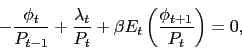
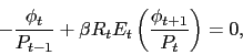
From (8), we get a usual Fisher
relation,
![\begin{displaymath} 1 = R_t E_t \left[\frac{\beta \phi_{t+1}}{\phi_t} \frac{1}{\pi_t}\right], \end{displaymath}](img69.gif)
|
(9) |
where
![]() is the gross rate of
price inflation between period
is the gross rate of
price inflation between period ![]() and period
and period
![]() . The stochastic discount factor
. The stochastic discount factor
![]() prices a
nominally risk-free one-period asset. Combining (5) and (7), we
get
prices a
nominally risk-free one-period asset. Combining (5) and (7), we
get
| (10) |
Substituting this expression into the previous one gives us the pricing formula for a one-period nominally risk-free bond,
![\begin{displaymath} 1 = R_t E_t \left[\frac{\beta u_{1t+1}}{u_{1t}} \frac{1}{\pi_{t+1}}\right]. \end{displaymath}](img75.gif)
As is standard in this type of cash/credit setup, the household first-order conditions also imply that the gross nominal interest rate equals the marginal rate of substitution between cash and credit goods,
In a monetary equilibrium, ![]() , otherwise
consumers could earn unbounded profits by buying money and selling
bonds.
, otherwise
consumers could earn unbounded profits by buying money and selling
bonds.
2.2 Production
The production side of the economy features a representative firm that must open vacancies, which entail costs, in order to hire workers and produce. The representative firm is ``large" in the sense that it operates many jobs and consequently has many individual workers attached to it through those jobs.
To be more specific, the firm requires only labor to produce its
output. The firm must engage in costly search for a worker to fill
each of its job openings. In each job ![]() that will
produce output, the worker and firm bargain over the pre-tax
nominal wage
that will
produce output, the worker and firm bargain over the pre-tax
nominal wage ![]() paid in that position. Output of
job
paid in that position. Output of
job ![]() is given by
is given by
![]() , which is subject to a
common technology realization
, which is subject to a
common technology realization ![]() . We allow for
curvature in
. We allow for
curvature in ![]() to enhance comparability with our
model in Section 5; of course, in
the model in this section, the curvature does not matter because
to enhance comparability with our
model in Section 5; of course, in
the model in this section, the curvature does not matter because
![]() is fixed anyway.
is fixed anyway.
Any two jobs ![]() and
and ![]() at the firm
are identical, so from here on we suppress the second subscript and
denote by
at the firm
are identical, so from here on we suppress the second subscript and
denote by ![]() the nominal wage in any job, and so
on. Total output of the firm thus depends on the production
technology and the measure of matches
the nominal wage in any job, and so
on. Total output of the firm thus depends on the production
technology and the measure of matches ![]() that
produce,
that
produce,
| (13) |
The total nominal wage paid by the firm in any given job is
![]() , and the total nominal wage bill
of the firm is the sum of wages paid at all of its positions,
, and the total nominal wage bill
of the firm is the sum of wages paid at all of its positions,
![]() .
.
The firm begins period ![]() with employment
stock
with employment
stock ![]() . Its future employment stock depends on
its current choices as well as the random matching process. With
probability
. Its future employment stock depends on
its current choices as well as the random matching process. With
probability ![]() , taken as given by the firm, a
vacancy will be filled by a worker. Labor-market tightness is
, taken as given by the firm, a
vacancy will be filled by a worker. Labor-market tightness is
![]() , and matching probabilities
depend only on tightness given the Cobb-Douglas matching function
we will assume.
, and matching probabilities
depend only on tightness given the Cobb-Douglas matching function
we will assume.
The firm also faces a cost of adjusting nominal wages. For each
of its workers, the real cost of changing nominal wages between
period ![]() and
and ![]() is
is
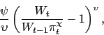
|
(14) |
where
![]() measures the degree to which
nominal wage adjustment is indexed to contemporaneous price
inflation. If
measures the degree to which
nominal wage adjustment is indexed to contemporaneous price
inflation. If ![]() , there is no indexation; if
, there is no indexation; if
![]() , there is full indexation; and if
, there is full indexation; and if
![]() , there is partial indexation.
There are two reasons we allow for indexation. First, there seems
to be a good deal of empirical support for wage indexation. Second,
comparing our steady-state results under full indexation and no
indexation allows us to disentangle some aspects of optimal policy
in our model.
, there is partial indexation.
There are two reasons we allow for indexation. First, there seems
to be a good deal of empirical support for wage indexation. Second,
comparing our steady-state results under full indexation and no
indexation allows us to disentangle some aspects of optimal policy
in our model.
If we use ![]() , which we do in the results we
report, then the cost function is of the Rotemberg quadratic
variety. We also explored the sensitivity of our results with
respect to values of
, which we do in the results we
report, then the cost function is of the Rotemberg quadratic
variety. We also explored the sensitivity of our results with
respect to values of ![]() around two and found
little difference. If
around two and found
little difference. If ![]() , clearly there is no
cost of wage adjustment. This Rotemberg type of nominal adjustment
cost specification is a fairly common convention in typical sticky
wage or sticky price models. At the expense of a heavier
computational burden, an alternative specification one may want to
pursue is a Calvo structure, in which wages in only a fraction of
jobs can be re-set every period. As we mentioned earlier, though,
our goal is not to provide a compelling micro-foundation for sticky
nominal wages; adopting a fairly-conventional reduced-form
specification is just a tractable way to get at our ultimate
objective. Part of our reason in choosing the Rotemberg approach is
that it makes solving our model computationally a bit easier
because it avoids the introduction of further leads and lags in
dynamic equations associated with a Calvo structure. Moreover, this
specification enhances comparability with the results in Chugh
(2006a), who uses a Rotemberg wage adjustment cost function.
, clearly there is no
cost of wage adjustment. This Rotemberg type of nominal adjustment
cost specification is a fairly common convention in typical sticky
wage or sticky price models. At the expense of a heavier
computational burden, an alternative specification one may want to
pursue is a Calvo structure, in which wages in only a fraction of
jobs can be re-set every period. As we mentioned earlier, though,
our goal is not to provide a compelling micro-foundation for sticky
nominal wages; adopting a fairly-conventional reduced-form
specification is just a tractable way to get at our ultimate
objective. Part of our reason in choosing the Rotemberg approach is
that it makes solving our model computationally a bit easier
because it avoids the introduction of further leads and lags in
dynamic equations associated with a Calvo structure. Moreover, this
specification enhances comparability with the results in Chugh
(2006a), who uses a Rotemberg wage adjustment cost function.
Regardless of whether or not nominal wages are costly to adjust,
wages are determined through bargaining, which we describe below.
In the firm's profit maximization problem, the wage-setting
protocol is taken as given. The firm thus chooses vacancies to post
![]() and future employment stock
and future employment stock ![]() to maximize discounted nominal profits starting at
date
to maximize discounted nominal profits starting at
date ![]() ,
,
![\begin{displaymath} E_t \sum_{s=0}^{\infty} \beta^s \left\{ \left(\frac{\beta \phi_{t+1+s}}{P_{t+s}}\right) \left[ P_{t+s} n_{t+s} z_{t+s} f(\bar{h}) - W_{t+s} n_{t+s} \bar{h} - \gamma P_{t+s} v_{t+s} - \frac{\psi}{\upsilon}\left(\frac{W_{t+s}}{W_{t+s-1} \pi_{t+s}^{\chi}}-1\right)^{\upsilon} n_{t+s} P_{t+s} \right] \right\}. \end{displaymath}](img109.gif)
The representative firm discounts period-![]() profits
using
profits
using
![]() because this is the
value to the household of receiving a unit of nominal
profit.5 In period
because this is the
value to the household of receiving a unit of nominal
profit.5 In period ![]() , the firm's
problem is thus to choose
, the firm's
problem is thus to choose ![]() and
and ![]() to maximize (15) subject to the law of
motion for employment
to maximize (15) subject to the law of
motion for employment
Firms incur the real cost ![]() for each
vacancy created, and job separation occurs with exogenous fixed
probability
for each
vacancy created, and job separation occurs with exogenous fixed
probability ![]() .
.
Associate the multiplier ![]() with the
employment constraint. The first-order conditions with respect to
with the
employment constraint. The first-order conditions with respect to
![]() and
and ![]() are,
respectively,
are,
respectively,
![\begin{displaymath} \frac{\mu_t \beta \phi_{t+1}}{P_t} = E_t \left[ \beta \left(\frac{\beta \phi_{t+2}}{P_{t+1}}\right)\left( z_{t+1} f(\bar{h}) - W_{t+1} \bar{h} - \frac{\psi}{\upsilon} \left(\frac{W_{t+1}}{W_t \pi_t^{\chi}}-1\right)^{\upsilon} P_{t+1} + (1-\rho^x) \mu_{t+1} \right) \right], \end{displaymath}](img127.gif)
Combining the optimality conditions (17) and (18) yields the job-creation condition
![\begin{displaymath} \frac{\gamma}{k^f(\theta_t)} = E_t \left[ \beta \left( \frac{\beta \phi_{t+2}}{\beta \phi_{t+1}}\right) (1-\rho^x) \left( z_{t+1} f(\bar{h}) - w_{t+1} \bar{h} - \frac{\psi}{\upsilon}\left(\frac{\pi^w_{t+1}}{\pi_t^{\chi}}-1\right)^{\upsilon} + \frac{\gamma}{k^f(\theta_{t+1})} \right) \right], \end{displaymath}](img129.gif)
where we have defined
![]() as the gross
nominal wage inflation rate and
as the gross
nominal wage inflation rate and
![]() is the real
wage rate. The job-creation condition states that at the optimal
choice, the vacancy-creation cost incurred by the firm is equated
to the discounted expected value of profits from the match. Profits
from a match take into account the wage cost of that match,
including future nominal wage adjustment costs, as well as future
marginal revenue product from the match. This condition is a
free-entry condition in the creation of vacancies and is one of the
critical equilibrium conditions of the model. In equilibrium,
is the real
wage rate. The job-creation condition states that at the optimal
choice, the vacancy-creation cost incurred by the firm is equated
to the discounted expected value of profits from the match. Profits
from a match take into account the wage cost of that match,
including future nominal wage adjustment costs, as well as future
marginal revenue product from the match. This condition is a
free-entry condition in the creation of vacancies and is one of the
critical equilibrium conditions of the model. In equilibrium,
![]() , which
can be seen from the household's optimality condition with respect
to credit good consumption, condition (6).
, which
can be seen from the household's optimality condition with respect
to credit good consumption, condition (6).
2.3 Government
The government's flow budget constraint is
| (20) |
Thus, the government finances its spending through labor income
taxation, issuance of nominal debt, and money creation. Note that
government consumption is a credit good, following Chari,
Christiano, and Kehoe (1991), because ![]() is not
paid for until period
is not
paid for until period ![]() . In equilibrium, the
government budget constraint can be expressed in real terms as
. In equilibrium, the
government budget constraint can be expressed in real terms as
where
![]() is the gross rate of
price inflation.
is the gross rate of
price inflation.
2.4 Nash Wage Bargaining
As is standard in the literature, we assume that the wage paid
in any given job is determined in a Nash bargain between a matched
worker and firm. Thus, the wage payment divides the match surplus.
Our departure from the standard Nash bargaining convention used in
the literature is that we assume bargaining occurs over the nominal
wage payment rather than the real wage payment. With zero costs of
wage adjustment, the real wage that emerges is identical to the one
that emerges from bargaining directly over the real wage. The
reason that nominal bargaining and real bargaining are identical if
wage adjustment is costless is straightforward. A firm and worker
in negotiations take the price level ![]() as given.
Bargaining over
as given.
Bargaining over ![]() thus pins down
thus pins down ![]() ;
alternatively, bargaining over
;
alternatively, bargaining over ![]() pins down
pins down
![]() . With no impediment to adjusting wages,
there is no problem adjusting either
. With no impediment to adjusting wages,
there is no problem adjusting either ![]() or
or
![]() to achieve some desired split of the
surplus, and the optimal split itself is independent of whether a
real unit of account or a nominal unit of account is used in
bargaining.
to achieve some desired split of the
surplus, and the optimal split itself is independent of whether a
real unit of account or a nominal unit of account is used in
bargaining.
In addition to bargaining over nominal wages, though, we assume
that nominal wage adjustment may entail a resource cost of the
Rotemberg-type described in Section 2.2. Details of the solution of the Nash
bargain with costly wage adjustment are given in
Appendix A. Here we present
only the outcome of the Nash bargain. Bargaining over the nominal
wage payment yields
![$\displaystyle { \frac{\omega_t}{1-\omega_t} \left[ z_t f(\bar{h}) - w_t \bar{h} - \frac{\psi}{\upsilon}\left(\frac{\pi^w_t}{\pi_t^{\chi}}-1\right)^{\upsilon} + \frac{\gamma}{k^f(\theta_t)}\right] = }$](img145.gif)
![$\displaystyle + (1-\theta_t k^f(\theta_t)) \beta E_t\left[\left(\frac{\omega_{t+1}}{1-\omega_{t+1}}\right) \left(\frac{u_{2t+1}}{u_{2t}}\right) (1-\rho^x) \left[z_{t+1} f(\bar{h}) - w_{t+1} \bar{h} - \frac{\psi}{\upsilon}\left(\frac{\pi^w_{t+1}}{\pi_{t+1}^{\chi}}-1\right)^{\upsilon} + \frac{\gamma}{k^f(\theta_{t+1})} \right] \right] ,$](img147.gif)
which characterizes the real wage ![]() agreed upon
in period
agreed upon
in period ![]() . In (22),
. In (22), ![]() is the
effective bargaining power of the worker and
is the
effective bargaining power of the worker and ![]() is the effective bargaining power of the firm.
Specifically,
is the effective bargaining power of the firm.
Specifically,

where ![]() and
and ![]() measure marginal changes in the value of a filled job and the value
of being employed, respectively, and
measure marginal changes in the value of a filled job and the value
of being employed, respectively, and ![]() is the
weight given to the worker's individual surplus in Nash
bargaining.6
is the
weight given to the worker's individual surplus in Nash
bargaining.6
As we say, we provide the details behind (22) and (23) in Appendix A, but there are three points worth
mentioning here. First, effective bargaining power ![]() is related to the Nash weight
is related to the Nash weight ![]() . With
flexible nominal wages and no labor taxation, it is straightforward
to show that
. With
flexible nominal wages and no labor taxation, it is straightforward
to show that
![]()
![]() (because in that case
(because in that case
![]() ). The presence of
proportional taxes and sticky wages drives a time-varying wedge
between
). The presence of
proportional taxes and sticky wages drives a time-varying wedge
between ![]() and
and ![]() . Second, the
expected future cost of adjusting the nominal wage affects the
time-
. Second, the
expected future cost of adjusting the nominal wage affects the
time-![]() wage payment. Third, the labor tax rate
appears in (22) both
directly as well as through effective bargaining power. The weight
wage payment. Third, the labor tax rate
appears in (22) both
directly as well as through effective bargaining power. The weight
![]() depends on
depends on ![]() ;
thus the weight
;
thus the weight ![]() , which affects the
time-
, which affects the
time-![]() split of the surplus, depends on
split of the surplus, depends on
![]() . Indeed, as can also be seen in
our Appendix A, if wages are
not at all sticky (
. Indeed, as can also be seen in
our Appendix A, if wages are
not at all sticky (![]() ), the bargaining weight
varies only because of variations in the tax rate,
), the bargaining weight
varies only because of variations in the tax rate,
The fact that current and future tax rates affect wage-setting may be important in understanding some of the results we present in Section 4.
2.5 Matching Technology
Matches between unemployed individuals searching for jobs and
firms searching to fill vacancies are formed according to a
matching technology, ![]() , where
, where ![]() is the number of searching individuals and
is the number of searching individuals and ![]() is the number of posted vacancies. A match formed in period
is the number of posted vacancies. A match formed in period
![]() will produce in period
will produce in period ![]() provided it survives exogenous separation at the beginning of
period
provided it survives exogenous separation at the beginning of
period ![]() . The evolution of total employment is
thus given by
. The evolution of total employment is
thus given by
2.6 Private-Sector Equilibrium
The equilibrium conditions of the model are the Fisher
equation (11) describing the
household's optimal intertemporal choices; the household
intratemporal optimality condition (12),
which is standard in cash/credit models; the restriction
![]() , which states that the net nominal
interest rate cannot be less than zero, a requirement for a
monetary equilibrium; the job-creation condition describing firm
profit-maximization
, which states that the net nominal
interest rate cannot be less than zero, a requirement for a
monetary equilibrium; the job-creation condition describing firm
profit-maximization
![\begin{displaymath} \frac{\gamma}{k^f(\theta_t)} = E_t \left[ \left( \frac{\beta u_{2t+1}}{u_{2t}}\right) (1-\rho^x) \left( z_{t+1} f(\bar{h}) - w_{t+1} \bar{h} - \frac{\psi}{\upsilon}\left(\frac{\pi^w_{t+1}}{\pi_{t+1}^{\chi}}-1\right)^{\upsilon} + \frac{\gamma}{k^f(\theta_{t+1})} \right) \right], \end{displaymath}](img179.gif)
in which the household discount factor for credit resources,
![]() , appears; the flow
government budget constraint, expressed in real
terms, (21) (in which we have
substituted
, appears; the flow
government budget constraint, expressed in real
terms, (21) (in which we have
substituted
![]() from (12) as well as the cash-in-advance
constraint (4) holding with
equality); the Nash wage characterized by (22); the law of motion for
employment (25); the
identity
from (12) as well as the cash-in-advance
constraint (4) holding with
equality); the Nash wage characterized by (22); the law of motion for
employment (25); the
identity
restricting the size of the labor force to one; a condition relating the rate of real wage growth to nominal price inflation and nominal wage inflation

and the resource constraint
Condition (28) is typically
thought of as an identity, but is one that does not hold trivially
in a model with nominally-rigid wages and thus must be included as
part of the description of equilibrium; see Chugh (2006a, p. 692)
for an intuitive explanation. In (29), total costs of posting vacancies
![]() are a resource cost for
the economy, as are wage adjustment costs; in the resource
constraint, we have made the substitution
are a resource cost for
the economy, as are wage adjustment costs; in the resource
constraint, we have made the substitution
![]() , eliminating
, eliminating ![]() from the set of endogenous processes of the model. The
private-sector equilibrium processes are thus
from the set of endogenous processes of the model. The
private-sector equilibrium processes are thus
![]() , for given processes
, for given processes
![]() .
.
3 Ramsey Problem in Basic Model
The problem of the Ramsey planner is to raise exogenous revenue
for the government through labor income taxes and money creation in
such a way that maximizes the welfare of the representative
household, subject to the equilibrium conditions of the economy. In
period zero, the Ramsey planner commits to a policy rule. Because
of the complexity of the model, we cast the Ramsey problem as one
of choosing both allocation and policy variables rather than in the
pure primal form often used in the literature, in which it is just
allocations that are chosen directly by the Ramsey planner. The
Ramsey problem is to choose
![]() to maximize (2) subject
to (11), (21), (22), (25), (26), (27), (28),
and (29) and taking as given
exogenous processes
to maximize (2) subject
to (11), (21), (22), (25), (26), (27), (28),
and (29) and taking as given
exogenous processes ![]() . In principle, we
must also impose the inequality condition
. In principle, we
must also impose the inequality condition
as a constraint on the Ramsey problem. This inequality constraint ensures (in terms of allocations -- refer to condition (12)) that the zero-lower-bound on the nominal interest rate is not violated. We thus refer to constraint (30) as the ZLB constraint. The ZLB constraint in general is an occasionally-binding constraint. Because our model likely is too complex, given current technology, to solve using global approximation methods that would be able to properly handle occasionally-binding constraints, for our dynamic results we drop the ZLB constraint and then check whether the ZLB constraint is ever violated. As we discuss when we present our parameterization in Section 4.1, using this approach raises an issue for one aspect of our model calibration.
Throughout, we assume that the first-order conditions of the Ramsey problem are necessary and sufficient and that all allocations are interior.
4 Optimal Policy in Basic Model
We characterize the Ramsey steady-state of our model numerically. Before turning to our results, we describe how we parameterize the model. Because a number of our steady-state results have a close analog in the optimal capital taxation results of Arseneau and Chugh (2006), we adopt, where possible, their calibration to enhance comparability.
4.1 Model Parameterization
We assume that the instantaneous utility function over cash and
credit goods is
![\begin{displaymath} u\left(c_{1t}, c_{2t}\right) = \frac{ \left\{\left[(1-\kappa)c_{1t}^{\phi} + \kappa c_{2t}^{\phi}\right]^{1/\phi}\right\}^{1-\sigma}-1}{1-\sigma}, \end{displaymath}](img193.gif)
|
(31) |
with, as is typical in cash/credit models, a CES aggregator over
cash and credit goods. For the aggregator, we adopt the calibration
used by Siu (2004) and Chugh (2006a, 2006b) and set ![]() and
and ![]() . The time unit of
the model is meant to be a quarter, so we set the subjective
discount factor to
. The time unit of
the model is meant to be a quarter, so we set the subjective
discount factor to ![]() , yielding an annual
real interest rate of about four percent. We set the curvature
parameter with respect to consumption to
, yielding an annual
real interest rate of about four percent. We set the curvature
parameter with respect to consumption to ![]() ,
consistent with many macro models.
,
consistent with many macro models.
Our timing assumptions are such that production in a period
occurs after the realization of separations. Following the
convention in the literature, we suppose that the unemployment rate
is measured before the realization of separations. We set
the quarterly probability of separation at ![]() , consistent with Shimer (2005). Thus, letting
, consistent with Shimer (2005). Thus, letting
![]() denote the steady-state level of
employment,
denote the steady-state level of
employment,
![]() is the employment rate, and
is the employment rate, and
![]() is the steady-state
unemployment rate.
is the steady-state
unemployment rate.
The match-level production function in general displays
diminishing returns in labor,
| (32) |
and we set the fixed number of hours a given individual works to
![]() , making our baseline model
comparable to our richer model in Section 5. In the richer model, we allow intensive
labor adjustment and calibrate utility parameters so that
steady-state hours are
, making our baseline model
comparable to our richer model in Section 5. In the richer model, we allow intensive
labor adjustment and calibrate utility parameters so that
steady-state hours are ![]() . Thus, we set
. Thus, we set
![]() here. Regarding curvature, we
choose
here. Regarding curvature, we
choose ![]() , a conventional value in DGE
models.7
, a conventional value in DGE
models.7
As in much of the literature, the matching technology is
Cobb-Douglas,
| (33) |
with the elasticity of matches with respect to the number of
unemployed set to ![]() , following
Blanchard and Diamond (1989), and
, following
Blanchard and Diamond (1989), and ![]() a
calibrating parameter that can be interpreted as a measure of
matching efficiency.
a
calibrating parameter that can be interpreted as a measure of
matching efficiency.
We normalize the utility of non-work to ![]() . With
this normalization, there are two natural cases to consider
regarding the calibration of
. With
this normalization, there are two natural cases to consider
regarding the calibration of ![]() , the disutility per
unit time of working. The first case is
, the disutility per
unit time of working. The first case is ![]() , so that
there is no difference at all in the realized welfare of employed
versus unemployed individuals. Although this calibration may not be
an accurate description of the relative welfare between unemployed
and employed individuals, it serves as a very useful benchmark for
our main results, as it did in Arseneau and Chugh (2006).
, so that
there is no difference at all in the realized welfare of employed
versus unemployed individuals. Although this calibration may not be
an accurate description of the relative welfare between unemployed
and employed individuals, it serves as a very useful benchmark for
our main results, as it did in Arseneau and Chugh (2006).
In the second case, we introduce ex-post heterogeneity between
employed and unemployed individuals by allowing ![]() to differ from
to differ from ![]() . As in Arseneau and
Chugh (2006), our choice of a specific value of
. As in Arseneau and
Chugh (2006), our choice of a specific value of ![]() is guided by Shimer (2005), who calibrates his model so that
unemployed individuals receive, in the form of unemployment
benefits, about 40 percent of the wages of employed individuals.
With his linear utility assumption, unemployed individuals are
therefore 40 percent as well off as employed persons. Our model
differs from Shimer's (2005) primarily in that we assume full
consumption insurance, but also in that we have curvature in
utility. Thus, when we allow for welfare heterogeneity, we
interpret Shimer's (2005) calibration to mean that unemployed
individuals must receive 2.5 times more consumption of both cash
goods and credit goods (in steady-state) than employed individuals
in order for the total utility of the two types of individuals to
be equalized. That is, we set
is guided by Shimer (2005), who calibrates his model so that
unemployed individuals receive, in the form of unemployment
benefits, about 40 percent of the wages of employed individuals.
With his linear utility assumption, unemployed individuals are
therefore 40 percent as well off as employed persons. Our model
differs from Shimer's (2005) primarily in that we assume full
consumption insurance, but also in that we have curvature in
utility. Thus, when we allow for welfare heterogeneity, we
interpret Shimer's (2005) calibration to mean that unemployed
individuals must receive 2.5 times more consumption of both cash
goods and credit goods (in steady-state) than employed individuals
in order for the total utility of the two types of individuals to
be equalized. That is, we set ![]() such that in
steady-state
such that in
steady-state
| (34) |
where ![]() denotes steady-state consumption,
denotes steady-state consumption,
![]() . The resulting value is
. The resulting value is ![]() , but we point out that our qualitative results do not
depend on the exact value of
, but we point out that our qualitative results do not
depend on the exact value of ![]() . As we discuss in
Section 4, all that is
important is that
. As we discuss in
Section 4, all that is
important is that ![]() .
.
We choose steady-state government purchases ![]() so that they constitute about 18 percent of total
output. The same value of
so that they constitute about 18 percent of total
output. The same value of ![]() (
(
![]() ) delivers a government share
of output very close to 18 percent in both models (as well as the
models in Section 5. Finally,
the steady-state value of government debt is to
) delivers a government share
of output very close to 18 percent in both models (as well as the
models in Section 5. Finally,
the steady-state value of government debt is to ![]() , making government debt about 40 percent of total
output in steady state, in line with the long-run average for the
U.S. economy.
, making government debt about 40 percent of total
output in steady state, in line with the long-run average for the
U.S. economy.
Regarding the Nash bargaining weight ![]() , we face a
bit of a tension, driven purely by practical concerns about solving
our model. We would like to focus on the case
, we face a
bit of a tension, driven purely by practical concerns about solving
our model. We would like to focus on the case
![]() so that the usual Hosios
(1990) parameterization is satisfied. The Nash bargaining weight
being a relatively esoteric parameter, it is hard to say whether
such a parameterization is empirically-justified. Nonetheless, it
is a parameterization of interest because many results in the
quantitative labor search literature are obtained assuming it. We
thus present our primary steady-state and dynamic results using
so that the usual Hosios
(1990) parameterization is satisfied. The Nash bargaining weight
being a relatively esoteric parameter, it is hard to say whether
such a parameterization is empirically-justified. Nonetheless, it
is a parameterization of interest because many results in the
quantitative labor search literature are obtained assuming it. We
thus present our primary steady-state and dynamic results using
![]() . However, when we turn to
dynamics, we run into a problem because with costless wage
adjustment and
. However, when we turn to
dynamics, we run into a problem because with costless wage
adjustment and ![]() , the zero-lower-bound on
the nominal interest rate is violated during simulations.8 For
the cases with costly wage adjustment, using
, the zero-lower-bound on
the nominal interest rate is violated during simulations.8 For
the cases with costly wage adjustment, using ![]() does not pose a problem. Rather than fiddle with
the calibration in an ad-hoc way to make the flexible-wage version
also satisfy the ZLB constraint, though, we simply present the
results as they are. We have reason to think that the main ideas
that emerge from our model are unaffected by this issue, but we
defer further discussion until our presentation of dynamic
results.
does not pose a problem. Rather than fiddle with
the calibration in an ad-hoc way to make the flexible-wage version
also satisfy the ZLB constraint, though, we simply present the
results as they are. We have reason to think that the main ideas
that emerge from our model are unaffected by this issue, but we
defer further discussion until our presentation of dynamic
results.
Finally, regarding the cost-adjustment parameter ![]() , we adopt Chugh's (2006a) calibration strategy and
consider four different values for our main results:
, we adopt Chugh's (2006a) calibration strategy and
consider four different values for our main results: ![]() (flexible wages),
(flexible wages), ![]() (nominal
wages sticky for two quarters on average),
(nominal
wages sticky for two quarters on average), ![]() (nominal wages sticky for three quarters on
average), and
(nominal wages sticky for three quarters on
average), and ![]() (nominal wages sticky for
four quarters on average). We recognize that Chugh's (2006a)
mapping of duration of wage-stickiness to the cost-adjustment
parameter may need to be modified because we have a fundamentally
different model, but we think it is a useful starting point and
allows us to demonstrate our main points. We leave an empirical
investigation of a ``wage Phillips curve" in the presence of labor
search frictions to future work.
(nominal wages sticky for
four quarters on average). We recognize that Chugh's (2006a)
mapping of duration of wage-stickiness to the cost-adjustment
parameter may need to be modified because we have a fundamentally
different model, but we think it is a useful starting point and
allows us to demonstrate our main points. We leave an empirical
investigation of a ``wage Phillips curve" in the presence of labor
search frictions to future work.
4.2 Ramsey Steady State
We begin by analyzing how costly nominal wage bargaining
influences allocations and policy variables in the Ramsey steady
state. We first discuss the case of no wage adjustment costs
(![]() ) and no wage indexation (
) and no wage indexation (![]() ) under our two alternative assumptions regarding the
value of
) under our two alternative assumptions regarding the
value of ![]() . These two sets of results serve as useful
benchmarks that will help in understanding how things change when
we introduce wage adjustment costs.
. These two sets of results serve as useful
benchmarks that will help in understanding how things change when
we introduce wage adjustment costs.
We provide a thorough analysis of how Ramsey policy operates in the long run because ours is one of the first studies of optimal policy in these types of models; as such, we think it worthwhile to spend some effort understanding the forces at work, knowing that future work will reveal some of these mechanisms to be more important than others. Readers primarily interested in understanding the dynamic policy implications of our model, however, may safely skip to Section 4.3 with the following summary of the steady-state results in mind. First, as is the case in the existing Ramsey literature, a tension between minimizing the monetary distortion (which in isolation calls for implementing the Friedman deflation) and minimizing the cost of nominal rigidities (which in isolation calls for implementing zero inflation) is present. In line with the existing literature, the tension is resolved overwhelmingly in favor of minimizing the distortions arising from nominal rigidities for even very small costs of wage adjustment. Second, and this is the most novel aspect of our steady-state results, the optimal inflation rate may actually be above zero, reflecting the consequences of a third force not present in standard models. This third force is that positive inflation can be used as an indirect way of addressing inefficiently-high job creation, an example of the inflation tax proxying for a missing tax instrument. In all cases, however, the steady-state inflation rate is never very far from zero.
4.2.1 No Adjustment Costs, No Indexation (
 )
)
Table 1 presents
steady-state allocations and policy variables under the Ramsey plan
assuming costless wage adjustment. The left panels of the table
present results for both ![]() and our benchmark
and our benchmark
![]() under the assumption that
under the assumption that ![]() With no utility heterogeneity between unemployed
and employed individuals, the Hosios condition delivers efficient
job creation, so the only concern of the Ramsey planner with regard
to monetary policy is minimizing the monetary distortion. It does
so by implementing the Friedman deflation, thereby driving the
nominal interest rate to zero and eliminating any wedge between
cash good consumption and credit good consumption. The government
budget constraint binds even though
With no utility heterogeneity between unemployed
and employed individuals, the Hosios condition delivers efficient
job creation, so the only concern of the Ramsey planner with regard
to monetary policy is minimizing the monetary distortion. It does
so by implementing the Friedman deflation, thereby driving the
nominal interest rate to zero and eliminating any wedge between
cash good consumption and credit good consumption. The government
budget constraint binds even though ![]() because,
with lump-sum instruments ruled out, a sustained deflation must be
financed by a small positive labor tax. This can be seen in the
first column of Table 1 which
shows that the labor tax is non-zero despite the fact that
because,
with lump-sum instruments ruled out, a sustained deflation must be
financed by a small positive labor tax. This can be seen in the
first column of Table 1 which
shows that the labor tax is non-zero despite the fact that
![]() .
.
With positive government spending and no costs of wage
adjustment, the Ramsey planner maintains the Friedman Rule. Doing
so merely crowds out private consumption and, despite the fact that
workers' effective bargaining power ![]() falls,
does not affect steady-state labor market allocations. In other
words, the proportional labor tax acts as a lump-sum instrument in
the special case of no wage adjustment costs and no welfare
heterogeneity. Cast in this light, the optimal financing problem
becomes quite transparent: the Ramsey planner chooses to finance
all government spending with the non-distortionary proportional
labor tax. This idea was developed in Arseneau and Chugh (2006) in
a non-monetary economy.
falls,
does not affect steady-state labor market allocations. In other
words, the proportional labor tax acts as a lump-sum instrument in
the special case of no wage adjustment costs and no welfare
heterogeneity. Cast in this light, the optimal financing problem
becomes quite transparent: the Ramsey planner chooses to finance
all government spending with the non-distortionary proportional
labor tax. This idea was developed in Arseneau and Chugh (2006) in
a non-monetary economy.
Next, we introduce welfare heterogeneity, so that ![]() ; results for this case are presented in the
right panels of Table 1. As
can be seen by comparing the
; results for this case are presented in the
right panels of Table 1. As
can be seen by comparing the ![]() columns in the
table, heterogeneity by itself lowers the bargained wage. The
reason for this, also developed in Arseneau and Chugh (2006), is
that individuals value the state of employment more highly and are
thus willing to accept a lower wage to move out of unemployment. As
the wage falls, the increased incentive for firms to post vacancies
results in inefficiently-high job creation. On balance, the
incentive to remove the monetary distortion remains; doing so
requires, as above, a positive labor tax to finance the Friedman
deflation. In the presence of heterogeneity, however, the labor tax
is distortionary. As the labor tax rises it erodes the bargaining
power of workers, thereby putting additional downward pressure on
the wage. This further fuels job creation, which is already
inefficiently high due to the presence of heterogeneity. Thus, the
optimal policy equates the marginal benefit of reducing the
monetary distortion to the marginal cost of further distorting the
labor market in order to finance the required deflation. With
flexible wages and
columns in the
table, heterogeneity by itself lowers the bargained wage. The
reason for this, also developed in Arseneau and Chugh (2006), is
that individuals value the state of employment more highly and are
thus willing to accept a lower wage to move out of unemployment. As
the wage falls, the increased incentive for firms to post vacancies
results in inefficiently-high job creation. On balance, the
incentive to remove the monetary distortion remains; doing so
requires, as above, a positive labor tax to finance the Friedman
deflation. In the presence of heterogeneity, however, the labor tax
is distortionary. As the labor tax rises it erodes the bargaining
power of workers, thereby putting additional downward pressure on
the wage. This further fuels job creation, which is already
inefficiently high due to the presence of heterogeneity. Thus, the
optimal policy equates the marginal benefit of reducing the
monetary distortion to the marginal cost of further distorting the
labor market in order to finance the required deflation. With
flexible wages and ![]() , the optimal policy calls
for a rate of inflation that is slightly above that implied by the
Friedman Rule, but the departure from the Friedman deflation is
obviously quantitatively very small.
, the optimal policy calls
for a rate of inflation that is slightly above that implied by the
Friedman Rule, but the departure from the Friedman deflation is
obviously quantitatively very small.
In the presence of heterogeneity, any incentive to inflate away
from the Friedman Rule in order to lower the labor tax rate is
completely overwhelmed if ![]() . With flexible
wages, the Ramsey planner implements the Friedman Rule and finances
all government expenditures through the labor tax. Thus, the costs
of reintroducing the monetary distortion are high relative to the
marginal improvement in the labor market that comes from easing off
on the rate of deflation and allowing the labor tax to fall by a
bit.
. With flexible
wages, the Ramsey planner implements the Friedman Rule and finances
all government expenditures through the labor tax. Thus, the costs
of reintroducing the monetary distortion are high relative to the
marginal improvement in the labor market that comes from easing off
on the rate of deflation and allowing the labor tax to fall by a
bit.
4.2.2 Adjustment Costs, No Indexation (
 )
)
We now analyze how the presence of costly nominal wage
adjustment influences the benchmark results presented above.
Figure 1 plots the key
Ramsey steady-state allocation and policy variables as a function
of the cost of adjustment parameter, ![]() , when
, when
![]() . Varying
. Varying
![]() varies the average length of
nominal wage-stickiness between zero and four quarters. As the
first two panels in the upper row of Figure 1 show, when
nominal wage adjustment is costly,
varies the average length of
nominal wage-stickiness between zero and four quarters. As the
first two panels in the upper row of Figure 1 show, when
nominal wage adjustment is costly, ![]() the
Friedman Rule ceases to be optimal. As
the
Friedman Rule ceases to be optimal. As ![]() rises, the
optimal rate of price inflation approaches zero. The reason behind
this result is well-understood: minimizing the resource cost of
nominal adjustment - be it nominal price adjustment or nominal wage
adjustment - is a quantitatively much more important goal of
optimal policy than is removing the monetary friction. This aspect
of our steady-state results echoes that of Schmitt-Grohe and Uribe
(2004b), Siu (2004), and Chugh (2006a).
rises, the
optimal rate of price inflation approaches zero. The reason behind
this result is well-understood: minimizing the resource cost of
nominal adjustment - be it nominal price adjustment or nominal wage
adjustment - is a quantitatively much more important goal of
optimal policy than is removing the monetary friction. This aspect
of our steady-state results echoes that of Schmitt-Grohe and Uribe
(2004b), Siu (2004), and Chugh (2006a).
The second row of Figure 1 shows a few
key labor market allocations. As ![]() increases, the
real wage rises and total employment and labor market tightness
each fall, although the effects are quantitatively small. This
labor market response stems from the fact that the resource costs
associated with nominal wage adjustment effectively shifts
bargaining power away from firms and towards workers. To understand
this point, consider how a change in
increases, the
real wage rises and total employment and labor market tightness
each fall, although the effects are quantitatively small. This
labor market response stems from the fact that the resource costs
associated with nominal wage adjustment effectively shifts
bargaining power away from firms and towards workers. To understand
this point, consider how a change in ![]() affects
workers' effective bargaining power
affects
workers' effective bargaining power ![]() as well
as the marginal change in the value of a filled job
as well
as the marginal change in the value of a filled job ![]() .9 As can be deduced from the derivation
of the Nash bargaining solution presented in Appendix A, in steady-state these partials
are
.9 As can be deduced from the derivation
of the Nash bargaining solution presented in Appendix A, in steady-state these partials
are
and
where we have used the fact that ![]() in steady
state and have left the indexation parameter
in steady
state and have left the indexation parameter ![]() in place. The important thing to note here is that the
sign of
in place. The important thing to note here is that the
sign of
![]() and hence
the sign of
and hence
the sign of
![]() may depend on
whether or not there is inflation or deflation in the steady state.
With no indexation (
may depend on
whether or not there is inflation or deflation in the steady state.
With no indexation (![]() ), if the steady state
features
), if the steady state
features ![]() , then
, then
![]() ,
implying
,
implying
![]() .10 Thus, with
deflation in the Ramsey steady state, which is indeed the case in
the absence of heterogeneity, a higher cost of wage adjustment
effectively transfers bargaining power away from firms and to
workers, resulting in higher real wages. The reason this transfer
of bargaining power occurs is because in a deflationary environment
with costly wage adjustment, raising the nominal wage by an
additional dollar pushes the absolute level of wage inflation
closer to zero, marginally reducing both current and expected
future costs of nominal wage adjustment. All else equal, the firm
benefits from this and is thus willing to cede a bit of bargaining
power in order to realize the cost savings. This effect gets
stronger as the costs of wage adjustment rise. Increased bargaining
power on the part of workers drives up the bargained wage, meaning
that an individual job is less profitable to a firm. Vacancy
postings fall and, as a consequence, both labor market tightness
and the total number of people working in the economy fall.
.10 Thus, with
deflation in the Ramsey steady state, which is indeed the case in
the absence of heterogeneity, a higher cost of wage adjustment
effectively transfers bargaining power away from firms and to
workers, resulting in higher real wages. The reason this transfer
of bargaining power occurs is because in a deflationary environment
with costly wage adjustment, raising the nominal wage by an
additional dollar pushes the absolute level of wage inflation
closer to zero, marginally reducing both current and expected
future costs of nominal wage adjustment. All else equal, the firm
benefits from this and is thus willing to cede a bit of bargaining
power in order to realize the cost savings. This effect gets
stronger as the costs of wage adjustment rise. Increased bargaining
power on the part of workers drives up the bargained wage, meaning
that an individual job is less profitable to a firm. Vacancy
postings fall and, as a consequence, both labor market tightness
and the total number of people working in the economy fall.
Next, turn to the case of welfare heterogeneity, so that
![]() . Figure 2 shows that, as
was the case in the absence of welfare heterogeneity, costly
nominal wage adjustment introduces an incentive to move toward zero
inflation because doing so minimizes the resource costs associated
with nominal wage adjustment. A notable difference, however, is
that with heterogeneity, as
. Figure 2 shows that, as
was the case in the absence of welfare heterogeneity, costly
nominal wage adjustment introduces an incentive to move toward zero
inflation because doing so minimizes the resource costs associated
with nominal wage adjustment. A notable difference, however, is
that with heterogeneity, as ![]() rises, the
Ramsey inflation rate actually moves above zero because anticipated
inflation is used to indirectly stifle job creation. The intuition
behind this result lies in a complicated interaction between
anticipated inflation, the costs of nominal wage adjustment, and
effective bargaining power. The Ramsey planner exploits this
interaction by using inflation to dampen the incentive for firms to
post vacancies. Doing so, however, involves incurring greater
resource costs associated with nominal wage adjustment. The optimal
inflation tax balances the welfare gain from mitigating
inefficiently-high job creation against the costs of nominal wage
adjustment that arise from doing so.
rises, the
Ramsey inflation rate actually moves above zero because anticipated
inflation is used to indirectly stifle job creation. The intuition
behind this result lies in a complicated interaction between
anticipated inflation, the costs of nominal wage adjustment, and
effective bargaining power. The Ramsey planner exploits this
interaction by using inflation to dampen the incentive for firms to
post vacancies. Doing so, however, involves incurring greater
resource costs associated with nominal wage adjustment. The optimal
inflation tax balances the welfare gain from mitigating
inefficiently-high job creation against the costs of nominal wage
adjustment that arise from doing so.
The precise economic mechanisms at work here seem to be quite
complex, but we can numerically verify our intuition by modifying
our model to allow the Ramsey planner to have access to a vacancy
tax. Following Domeij (2005) and Arseneau and Chugh (2006), we
replace ![]() with
with
![]() in the firm's profit
function and the resulting job-creation condition, and we introduce
in the firm's profit
function and the resulting job-creation condition, and we introduce
![]() as a revenue item in the
government budget constraint, where
as a revenue item in the
government budget constraint, where ![]() is a
proportional vacancy tax rate. If
is a
proportional vacancy tax rate. If ![]() , the firm must pay a tax for each vacancy it
created, while if
, the firm must pay a tax for each vacancy it
created, while if ![]() , the firm
receives a subsidy for each vacancy. Note that the total vacancy
tax adds to government revenues and is now part of the optimal
financing problem.
, the firm
receives a subsidy for each vacancy. Note that the total vacancy
tax adds to government revenues and is now part of the optimal
financing problem.
The vacancy tax offers the Ramsey planner a more efficient
instrument with which to correct the labor market distortion. Thus,
if our intuition about why inflation is above zero for high enough
![]() without a vacancy tax is correct, the
optimal policy mix in the presence of a vacancy tax should involve
slight deflation (reflecting the usual tradeoff between the
monetary distortion and the resource costs of wage adjustment) and
a positive vacancy tax (reflecting the fundamental labor market
distortion). As shown in the bottom right panel of
Table 1, numerical results
support our conjecture; in the cases in which long-run inflation
was positive with no vacancy tax available, inflation is now
between zero and the Friedman Rule and there is a tax on vacancy
creation. Having demonstrated that positive inflation rates act as
a proxy for a vacancy tax, we now continue our analysis by again
omitting the direct vacancy instrument. Some justification for this
might be that, given how much attention is usually paid to
promoting job creation, an explicit vacancy tax may be
politically infeasible.
without a vacancy tax is correct, the
optimal policy mix in the presence of a vacancy tax should involve
slight deflation (reflecting the usual tradeoff between the
monetary distortion and the resource costs of wage adjustment) and
a positive vacancy tax (reflecting the fundamental labor market
distortion). As shown in the bottom right panel of
Table 1, numerical results
support our conjecture; in the cases in which long-run inflation
was positive with no vacancy tax available, inflation is now
between zero and the Friedman Rule and there is a tax on vacancy
creation. Having demonstrated that positive inflation rates act as
a proxy for a vacancy tax, we now continue our analysis by again
omitting the direct vacancy instrument. Some justification for this
might be that, given how much attention is usually paid to
promoting job creation, an explicit vacancy tax may be
politically infeasible.
4.2.3 Full Wage Indexation 
The results so far have all been under the assumption of no
indexation (![]() ) and show that the optimal rate
of steady-state inflation is highly sensitive to the costs of
nominal wage adjustment. This raises the question of whether or not
these results are robust to wage indexation.
Expression (36) shows that if
) and show that the optimal rate
of steady-state inflation is highly sensitive to the costs of
nominal wage adjustment. This raises the question of whether or not
these results are robust to wage indexation.
Expression (36) shows that if
![]() ,
,
![]() , implying
, implying
![]() . With full
indexation, effective bargaining power is invariant to the costs of
nominal wage adjustment.
. With full
indexation, effective bargaining power is invariant to the costs of
nominal wage adjustment.
Figure 3 summarizes how
steady-state inflation depends on ![]() when the
Ramsey planner must finance positive government expenditures. If
nominal wages are unindexed to price inflation, the optimal rate of
inflation rises away from the Friedman Rule as the costs of wage
adjustment rise. In contrast, with full wage indexation, the
Friedman Rule is always optimal regardless of assumptions regarding
heterogeneity. Partial indexation, meaning
when the
Ramsey planner must finance positive government expenditures. If
nominal wages are unindexed to price inflation, the optimal rate of
inflation rises away from the Friedman Rule as the costs of wage
adjustment rise. In contrast, with full wage indexation, the
Friedman Rule is always optimal regardless of assumptions regarding
heterogeneity. Partial indexation, meaning ![]() , would lead to an optimal rate of inflation
that is simply a convex combination of these two cases, putting
steady state inflation somewhere between the Friedman deflation and
the solid or dotted lines shown in Figure 3 for a given
level of
, would lead to an optimal rate of inflation
that is simply a convex combination of these two cases, putting
steady state inflation somewhere between the Friedman deflation and
the solid or dotted lines shown in Figure 3 for a given
level of ![]() . We proceed from here on assuming no
indexation (
. We proceed from here on assuming no
indexation (![]() ) because it simplifies obtaining
dynamic results.
) because it simplifies obtaining
dynamic results.
4.3 Ramsey Dynamics
To study dynamics, we approximate our model by linearizing in
levels the Ramsey first-order conditions for time ![]() around the non-stochastic steady-state of these
conditions. Our numerical method is our own implementation of the
perturbation algorithm described by Schmitt-Grohe and Uribe
(2004c). As in Khan, King, and Wolman (2003) and others, we assume
that the initial state of the economy is the asymptotic Ramsey
steady state. Throughout, we assume, as is common in the
literature, that the first-order conditions of the Ramsey problem
are necessary and sufficient and that all allocations are interior.
We also point out that because we assume full commitment on the
part of the Ramsey planner, the use of state-contingent inflation
is not a manifestation of time-inconsistent policy. The ``surprise"
in surprise inflation is due solely to the unpredictable components
of government spending and technology and not due to a retreat on
past promises.
around the non-stochastic steady-state of these
conditions. Our numerical method is our own implementation of the
perturbation algorithm described by Schmitt-Grohe and Uribe
(2004c). As in Khan, King, and Wolman (2003) and others, we assume
that the initial state of the economy is the asymptotic Ramsey
steady state. Throughout, we assume, as is common in the
literature, that the first-order conditions of the Ramsey problem
are necessary and sufficient and that all allocations are interior.
We also point out that because we assume full commitment on the
part of the Ramsey planner, the use of state-contingent inflation
is not a manifestation of time-inconsistent policy. The ``surprise"
in surprise inflation is due solely to the unpredictable components
of government spending and technology and not due to a retreat on
past promises.
We conduct 5000 simulations, each 100 periods long. To make the
comparisons meaningful as we vary ![]() , the same
realizations for government spending shocks and productivity shocks
are used across versions of our model. We limit the length of each
repetition because, as the results below show, there is a near-unit
root in real government debt and thus we must prevent the model
from wandering too far from initial conditions. For each
simulation, we then compute first and second moments and report the
medians of these moments across the 5000 simulations. By averaging
over so many short-length simulations, we are likely obtaining a
fairly accurate description of model dynamics even if a handful of
simulations drift far away from the steady state.
, the same
realizations for government spending shocks and productivity shocks
are used across versions of our model. We limit the length of each
repetition because, as the results below show, there is a near-unit
root in real government debt and thus we must prevent the model
from wandering too far from initial conditions. For each
simulation, we then compute first and second moments and report the
medians of these moments across the 5000 simulations. By averaging
over so many short-length simulations, we are likely obtaining a
fairly accurate description of model dynamics even if a handful of
simulations drift far away from the steady state.
Table 2 presents simulation-based moments for the key policy and allocation variables of our model for various degrees of nominal wage rigidity. We divide the discussion of results into two parts: first, we analyze the dynamics of policy variables, and then we discuss the dynamics of labor market variables. The important link between the dynamics of policy variables and the dynamics of labor market variables is the dynamics of the real wage. As we pointed our earlier, we face an issue regarding the zero-lower-bound in our flexible-wage model; we discuss this issue below.
4.3.1 Policy Dynamics
The top panel of Table 2 shows that if
nominal wages are costless to adjust, the average level of
inflation is near the Friedman deflation and price inflation
volatility is quite high. The basic reason for inflation volatility
with flexible wages and prices, as mentioned in the introduction
and as is well-known in the Ramsey literature, is that the Ramsey
planner finds price-level variations a relatively costless way of
financing innovations to the government budget. Ex-post inflation
renders nominally risk-free debt payments state-contingent in real
terms. In the basic Ramsey literature, generating this ex-post
variation in debt returns via unanticipated inflation allows the
planner to finance a large share of innovations to the government
budget without changing the labor tax rate very much. A
tax-smoothing incentive is thus the source of inflation volatility
in a basic Ramsey model. However, as Table 2 shows, with
![]() our model displays a fair amount of
tax rate variability, an order of magnitude larger than in a basic
Ramsey model.11 We discuss this point further below.
With
our model displays a fair amount of
tax rate variability, an order of magnitude larger than in a basic
Ramsey model.11 We discuss this point further below.
With ![]() , nominal wage inflation is also
quite volatile; coupled with volatile price inflation, the path for
the real wage turns out to be relatively stable, with a standard
deviation of about 1 percent, much less than the volatility of
output, which has a standard deviation of about 1.8
percent.12
, nominal wage inflation is also
quite volatile; coupled with volatile price inflation, the path for
the real wage turns out to be relatively stable, with a standard
deviation of about 1 percent, much less than the volatility of
output, which has a standard deviation of about 1.8
percent.12
If nominal wages are instead costly to adjust, wage inflation is near zero with very low variability. The reason behind low and stable nominal wage inflation is that the Ramsey planner largely eliminates the direct resource cost changes in nominal wages entail. However, the underlying incentive for the planner to generate movements in the price level is of course still present. The tradeoff thus facing the planner is the welfare loss due to any induced volatility in the real wage versus the welfare gain due to the shock absorption afforded by state-contingent inflation. In our model, relatively large fluctuations in the real wage apparently do not affect welfare very much, so price inflation continues to be quite volatile. This result is directly opposite that in Chugh (2006a), who finds that even two quarters of nominal wage rigidity lowers price inflation volatility by an order of magnitude. With two or three quarters of nominally-rigid wages on average, we find that price inflation volatility is still around five percent, little changed from the fully-flexible case. With four quarters of wage stickiness, inflation volatility is actually higher than in the fully-flexible case, and wage inflation volatility rises a bit as well compared to the two-quarter and three-quarter cases. Comparing our results with those of Chugh (2006a), it clearly matters for prescriptions regarding optimal inflation in what type of underlying environment -- a Walrasian labor market or a labor market with fundmental frictions -- nominal wage rigidity is modeled. This is the central result of our study.
There are other novel aspects of the dynamic Ramsey policy in this model, as well. The labor tax rate fluctuates around its steady-state value of about 23 percent. However, as noted above, its volatility is different than in basic Ramsey models. With flexible wages, the standard deviation of the tax rate is over one percent, an order of magnitude higher than benchmark tax-smoothing results in the Ramsey literature. In basic Ramsey models, the planner refrains from tax rate variability because doing so would disrupt equilibrium marginal rates of substitution between consumption and leisure, which harms welfare; shocks to the government budget are instead financed by varying realized returns on nominal government debt via state-contingent variations in the price level. In contrast, our results show that variability of proportional labor taxes are not as undesirable in a bargaining framework because there is no margin that is directly affected by the tax rate. The tax rate affects the bargained wage, which in turn influences the evolution of expected future wages, which in turn affects vacancy-postings by firms. This mechanism by which variations in taxes affect allocations apparently has very different quantitative welfare consequences than in models with standard Walrasian labor markets. Furthermore, the fact that our flexible-wage model predicts a more volatile tax rate than do basic Ramsey models may be related to the result that inflation is a bit less variable than in basic Ramsey models. For comparison, in standard flexible-price/flexible-wage Ramsey models without capital, Chari, Christiano, and Kehoe (1991) report inflation volatility of about 20 percent, while Schmitt-Grohe and Uribe (2004b), Siu (2004), and Chugh (2006a) all report inflation volatility of about 7 percent. The dynamic tradeoff in our model thus falls a little more on the side of tax variability and a little less on the side of inflation variability; nonetheless, we would call a standard deviation of inflation of nearly 5 percent quite volatile.13 The tax rate becomes more volatile as the costs of nominal adjustment rise; this finding is line with Schmitt-Grohe and Uribe (2004b), Siu (2004), and Chugh (2006a).
To try to shed a little more light on why tax rate variability
is not so undesirable in our model, consider the time-![]() wage payment described by (22). This sharing rule reveals
that the way in which variations in the labor tax rate influence
allocations in our model is very different than in standard models.
In a standard model, a labor tax creates only a static wedge. With
our bargaining specification, both
wage payment described by (22). This sharing rule reveals
that the way in which variations in the labor tax rate influence
allocations in our model is very different than in standard models.
In a standard model, a labor tax creates only a static wedge. With
our bargaining specification, both ![]() and
and
![]() affect the time-
affect the time-![]() split of the match surplus through their influences on period
split of the match surplus through their influences on period
![]() and
and ![]() effective
bargaining weights. In addition, if
effective
bargaining weights. In addition, if ![]() ,
price inflation and nominal wage inflation also influence the
split. The last row in each panel of Table 2 shows the
dynamics of the worker's effective bargaining power
,
price inflation and nominal wage inflation also influence the
split. The last row in each panel of Table 2 shows the
dynamics of the worker's effective bargaining power ![]() (defined in expression (23)). The mean and persistence of worker
effective bargaining power are essentially invariant to the
stickiness of nominal wages. In line with how the variability of
the tax rate changes, though,
(defined in expression (23)). The mean and persistence of worker
effective bargaining power are essentially invariant to the
stickiness of nominal wages. In line with how the variability of
the tax rate changes, though, ![]() becomes more
volatile as
becomes more
volatile as ![]() rises. Figure 4 presents dynamic
realizations of
rises. Figure 4 presents dynamic
realizations of ![]() and
and ![]() from one simulation for various degrees of nominal wage rigidity.
With
from one simulation for various degrees of nominal wage rigidity.
With ![]() , there is a negative linear relation
between the two, as expression (24) confirms there should be.
With
, there is a negative linear relation
between the two, as expression (24) confirms there should be.
With ![]() , it is harder to analytically see
the relation between
, it is harder to analytically see
the relation between ![]() and
and ![]() because variations in
because variations in ![]() affect
the relationship as well. However, Figure 5
shows there is virtually no dynamic relationship between realized
inflation and
affect
the relationship as well. However, Figure 5
shows there is virtually no dynamic relationship between realized
inflation and ![]() no matter the degree of wage
rigidity. In conjunction with Figure 5,
Figure 4 then suggests
that the dynamics of
no matter the degree of wage
rigidity. In conjunction with Figure 5,
Figure 4 then suggests
that the dynamics of ![]() can still be thought of
as being driven primarily by the dynamics of
can still be thought of
as being driven primarily by the dynamics of ![]() , evidenced by the continued negative relationship
between the two even as wages become more costly to adjust.
Time-variation in
, evidenced by the continued negative relationship
between the two even as wages become more costly to adjust.
Time-variation in ![]() affects how the
surplus is divided between a worker and a firm; splits of the
surplus have little to do with economic efficiency, and it is
economic efficiency that is a primitive concern of the Ramsey
planner, not the split of the surplus. Loosely speaking, our
interpretation of our results is thus that tax rate variability is
tolerable because all it does is affect the split of the surplus,
not allocations.
affects how the
surplus is divided between a worker and a firm; splits of the
surplus have little to do with economic efficiency, and it is
economic efficiency that is a primitive concern of the Ramsey
planner, not the split of the surplus. Loosely speaking, our
interpretation of our results is thus that tax rate variability is
tolerable because all it does is affect the split of the surplus,
not allocations.
Real government debt obligations, defined as
![]() , display a near-unit
root no matter the degree of nominal rigidity. At first glance,
this result does not seem readily reconcilable with existing
results in the Ramsey literature. Aiyagari et al (2002) showed that
incomplete (real) government bond markets render government debt
highly persistent.14 Schmitt-Grohe and Uribe (2004b) and
Siu (2004) subsequently demonstrated that with sticky nominal
prices and nominally-riskless government debt, real debt exhibits
the same property. Chugh (2006a) shows that nominally-rigid wages,
even with fully-flexible prices, also impart this feature to
optimal policy. This set of results leave the impression that it is
something about the presence of nominal rigidities per se
(or, more precisely, the inability or undesirability of making real
debt payments state-contingent) that renders real debt highly
persistent. In our model, debt is highly persistent even with no
nominal friction. A common theme running through the results in the
existing literature is that a near-unit root in government debt is
associated with relatively high variability in labor tax rates. Our
model, including, notably, our flexible-wage model, exhibits this
association. Indeed, high persistence of government debt goes
hand-in-hand with high measured variability of the tax rate.
Figure 6 shows the labor
tax rate and real government debt obligations from a representative
simulation (the same simulation underlying Figures 4
and 5) of our
flexible-wage model. The tax rate is quite stable around 23 percent
until about period 55, when it enters a large cyclical downswing,
at the same time real debt enters a persistent upswing; high
government debt allows for low taxes. As we just discussed,
however, swings in tax rates do not seem to be as
welfare-diminishing in our model as in basic models.
, display a near-unit
root no matter the degree of nominal rigidity. At first glance,
this result does not seem readily reconcilable with existing
results in the Ramsey literature. Aiyagari et al (2002) showed that
incomplete (real) government bond markets render government debt
highly persistent.14 Schmitt-Grohe and Uribe (2004b) and
Siu (2004) subsequently demonstrated that with sticky nominal
prices and nominally-riskless government debt, real debt exhibits
the same property. Chugh (2006a) shows that nominally-rigid wages,
even with fully-flexible prices, also impart this feature to
optimal policy. This set of results leave the impression that it is
something about the presence of nominal rigidities per se
(or, more precisely, the inability or undesirability of making real
debt payments state-contingent) that renders real debt highly
persistent. In our model, debt is highly persistent even with no
nominal friction. A common theme running through the results in the
existing literature is that a near-unit root in government debt is
associated with relatively high variability in labor tax rates. Our
model, including, notably, our flexible-wage model, exhibits this
association. Indeed, high persistence of government debt goes
hand-in-hand with high measured variability of the tax rate.
Figure 6 shows the labor
tax rate and real government debt obligations from a representative
simulation (the same simulation underlying Figures 4
and 5) of our
flexible-wage model. The tax rate is quite stable around 23 percent
until about period 55, when it enters a large cyclical downswing,
at the same time real debt enters a persistent upswing; high
government debt allows for low taxes. As we just discussed,
however, swings in tax rates do not seem to be as
welfare-diminishing in our model as in basic models.
The dynamics of taxes and real government debt thus seem to be
driven by a dynamic bargaining power effect - that is, by the
(Ramsey-optimal) fluctuations in ![]() . We do not
claim we yet fully understand the nature of this dynamic bargaining
power effect, but we think studying how bargaining and
policy-setting interact seems an interesting future avenue of
research.
. We do not
claim we yet fully understand the nature of this dynamic bargaining
power effect, but we think studying how bargaining and
policy-setting interact seems an interesting future avenue of
research.
The first panel of Table 2 indicates
that the zero-lower-bound is violated during simulations of the
flexible-wage version of our model. Recall from our analysis of the
steady state that the Friedman Rule is optimal with flexible wages.
Without handling the occasionally-binding ZLB
constraint (30), which our dynamic
numerical implementation does not, the nominal interest rate is
free to go below zero. The fluctuations are not very large, but,
because technically the simulations violate the conditions of a
monetary equilibrium, one may be inclined to not place too much
faith in the results from the flexible-wage simulations. We think
the results are still interpretable, however, because if we raise
the Nash weight ![]() on the worker's surplus and
simulate the flexible-wage version of our model, we find a
steady-state deviation from the Friedman Rule and no dynamic
violations of the zero lower bound.15 For
on the worker's surplus and
simulate the flexible-wage version of our model, we find a
steady-state deviation from the Friedman Rule and no dynamic
violations of the zero lower bound.15 For ![]() , not too far above our preferred Hosios
parameterization, we find that the zero-lower-bound is never
violated dynamically and the cyclical properties of policy and
quantity variables are very close to those presented in
Table2. Thus, the
general picture emerging from our model does not hinge on properly
handling the ZLB constraint. To avoid yet another fundamental
distortion in our model, though, we have chosen to focus on just
the
, not too far above our preferred Hosios
parameterization, we find that the zero-lower-bound is never
violated dynamically and the cyclical properties of policy and
quantity variables are very close to those presented in
Table2. Thus, the
general picture emerging from our model does not hinge on properly
handling the ZLB constraint. To avoid yet another fundamental
distortion in our model, though, we have chosen to focus on just
the ![]() case.16
case.16
The evolution of real wage payments is critical in understanding
why the Ramsey planner continues to implement highly variable
inflation as ![]() rises. With volatile price inflation
and quite stable nominal wage inflation, real wage volatility rises
as
rises. With volatile price inflation
and quite stable nominal wage inflation, real wage volatility rises
as ![]() rises: moving from fully-flexible wages
to four quarters of wage stickiness, the volatility of the real
wage increases three-fold. However, the consequences of this
increase in real wage variability on labor market outcomes is
negligible, as we discuss in the next section, and this is the
reason that optimal inflation volatility remains high no matter the
degree of nominal wage rigidity.
rises: moving from fully-flexible wages
to four quarters of wage stickiness, the volatility of the real
wage increases three-fold. However, the consequences of this
increase in real wage variability on labor market outcomes is
negligible, as we discuss in the next section, and this is the
reason that optimal inflation volatility remains high no matter the
degree of nominal wage rigidity.
4.3.2 Labor Market Dynamics
The volatility of unemployment, vacancies, and labor market tightness predicted by labor search models has received much attention lately. Since Shimer (2005) and Hall (2005) pointed out that the basic labor search model with Nash bargaining predicts far too little volatility in these labor market measures compared to empirical evidence, many studies have tried to address this issue. The main line of attack on this question has been to investigate the consequences of alternative (real) wage-setting mechanisms because, as Shimer (2005) pointed out, wage dynamics emerging from Nash bargaining are the root cause of the problem.17 Here, we assess what happens to the volatility of these measures under the optimal policy as the degree of nominal wage rigidity varies.
Table 2 shows that
the standard deviations of unemployment (which can be inferred from
the volatility of employment, ![]() ), vacancies, and
labor-market tightness (
), vacancies, and
labor-market tightness (![]() ) are all smallest when
there are no costs of nominal wage adjustment. In terms of relative
volatilities (relative to the volatility of output), unemployment
is about 80 percent as volatile as output, vacancies are about 30
percent as volatile as output, and tightness is about 80 percent as
volatile as output.18 Compared to the empirical evidence
reported by Gertler and Trigari (2006), the volatilities of each of
these variables in the flexible-wage version of our model is
substantially lower than in the data; this, in fact, is simply the
Shimer (2005) critique.19
) are all smallest when
there are no costs of nominal wage adjustment. In terms of relative
volatilities (relative to the volatility of output), unemployment
is about 80 percent as volatile as output, vacancies are about 30
percent as volatile as output, and tightness is about 80 percent as
volatile as output.18 Compared to the empirical evidence
reported by Gertler and Trigari (2006), the volatilities of each of
these variables in the flexible-wage version of our model is
substantially lower than in the data; this, in fact, is simply the
Shimer (2005) critique.19
With costs of nominal wage adjustment, the volatilities of all
of these variables rise, but only slightly. Indeed, once nominal
wages are at all sticky, the volatilites of these variables do not
change much with ![]() . At the same time, the real wage
becomes quite a bit more volatile as
. At the same time, the real wage
becomes quite a bit more volatile as ![]() rises: its
volatility is 50 percent higher with three quarters of nominal wage
stickiness than with flexible wages and about three times more
volatile with four quarters of wage stickiness. This result goes in
the opposite direction of the recent thrust in the literature that
explores mechanisms to make real wages less volatile and
quantity variables more volatile. As we mentioned in the
introduction, we do not view this as a problematic prediction of
our model because our primary concern is not explaining the data.
We are interested in understanding optimal policy, and the reason
that real wages become more volatile as
rises: its
volatility is 50 percent higher with three quarters of nominal wage
stickiness than with flexible wages and about three times more
volatile with four quarters of wage stickiness. This result goes in
the opposite direction of the recent thrust in the literature that
explores mechanisms to make real wages less volatile and
quantity variables more volatile. As we mentioned in the
introduction, we do not view this as a problematic prediction of
our model because our primary concern is not explaining the data.
We are interested in understanding optimal policy, and the reason
that real wages become more volatile as ![]() rises --
namely, because the Ramsey planner keeps nominal price inflation
volatility high even while muting nominal wage inflation volatility
-- is clear. We think it is useful to know that inducing more
volatile real wages in the face of rigid nominal wages is in fact
the optimal thing to do if one believes this class of models is
useful for studying policy, regardless of what the data say.
Indeed, in this sense, our results echo those of Erceg, Henderon,
and Levin (2000).
rises --
namely, because the Ramsey planner keeps nominal price inflation
volatility high even while muting nominal wage inflation volatility
-- is clear. We think it is useful to know that inducing more
volatile real wages in the face of rigid nominal wages is in fact
the optimal thing to do if one believes this class of models is
useful for studying policy, regardless of what the data say.
Indeed, in this sense, our results echo those of Erceg, Henderon,
and Levin (2000).
Perhaps the most interesting aspect of this result is that highly volatile real wages seem to harm welfare so little in this model of labor markets. The reason for this is that the actual real wage simply divides the existing surplus between a matched worker and firm and has little to do with the formation of the match in the first place.20 As Hall (2005) stressed, given that a match exists, there is a continuum of real wages, bounded by the threat points (outside values) of the parties, that are acceptable to both the worker and the firm. In implementing optimal policy, the Ramsey planner exploits this feature of equilibrium in generating state-contingent inflation, which in turn leads to state-contingent movements in the realized real wage and thus state-contingent splits of the surplus. Efficiency and the efficient tax mix of course have nothing to say about how rents are divided amongst parties. This is somewhat of a restatement of our earlier point that movements in the labor tax rate are not terribly disruptive in our model because they primarily just lead to movements in effective bargaining power, which also lead only to movements in how rents are divided amongst parties.
Finally, because the labor search model is so well-suited to thinking about issues regarding unemployment, one may wonder whether a Phillips Curve arises in our model. Figure 7 shows a negative relationship between cyclical inflation rates and cylical unemployment rates does arise if wages are flexible. However, this Phillips relation is not a feature of optimal policy with sticky nominal wages.
In summary, our results so far suggest that if the realized real wage did affect allocations more directly than they do in the model we have developed so far, then the optimal degree of price inflation volatility may fall as the cost of nominal wage adjustment rises. In Section 5 we pursue this idea by introducing an intensive margin of labor adjustment that potentially is affected by the realized real wage.
5 Intensive Margin
The way in which we introduce an hours margin follows closely that of Arseneau and Chugh (2006), who in turn build on Trigari (2006). The basic reason why we explore the consequences of allowing an intensive margin is that it potentially re-introduces to the model a neoclassical mechanism regarding a component -- the hours choice -- of labor supply. To the extent that the real wage does affect labor supply along the neoclassical intensive margin, we might expect to find that inflation volatility and/or tax-rate variability is welfare-diminishing, in contrast to the main findings in our basic model.
We consider three protocols by which hours are determined: simultaneous Nash bargaining between the firm and the worker over both hours and the wage payment; a right-to-manage (RTM) system in which the firm unilaterally sets its workers' hours, taking as given the bargained wage; and a right-to-work (RTW) convention in which each individual worker unilaterally chooses how many hours he works, taking as given the bargained wage. Of these three conventions, the latter two are the most likely candidates to make real wage fluctuations costly (precisely because in each case some party chooses hours taking as given the contemporaneous real wage) and thus dampen inflation volatility. Our results show that inflation volatility is indeed dampened in these two cases, but still remains quite high.
5.1 Modifications to the Model
We briefly describe the main modifications to the basic model of Section 2 and relegate to Appendix B the implementation details behind each hours-determination arrangement. As we mention below and show more fully in Appendix B, the differences between the three models of hours-determination essentially lie in differences in effective bargaining weights of workers and firms.
5.1.1 Households
Suppose an individual family member who works ![]() hours experiences disutility of effort
hours experiences disutility of effort ![]() that
varies with hours. Thus, total household utility is
that
varies with hours. Thus, total household utility is
![\begin{displaymath} E_0 \sum_{t=0}^{\infty} \beta^t \left[u(c_{1t},c_{2t}) - \int_0^{n_t} e(h^i_t) di + \int_{n_t}^1 v^i di \right]. \end{displaymath}](img334.gif)
|
(37) |
In the household's budget constraint (3), we replace ![]() by
by
![]() . Once again, we assume symmetry amongst
all employed individuals and amongst all unemployed individuals, so
household utility can be expressed as
. Once again, we assume symmetry amongst
all employed individuals and amongst all unemployed individuals, so
household utility can be expressed as
![\begin{displaymath} E_0 \sum_{t=0}^{\infty} \beta^t \left[u(c_{1t},c_{2t}) - n_t e(h_t) + (1-n_t)v \right]. \end{displaymath}](img337.gif)
|
(38) |
5.1.2 Firms
Each filled job now produces output
![]() ; with symmetry across
all jobs, total output of the firm is
; with symmetry across
all jobs, total output of the firm is
![]() .
.
5.1.3 Bargaining Over Hours
The first hours-determination scheme we consider is that the
firm and worker (Nash) bargain simultaneously over the wage payment
and hours. This setup is quite common in labor search models with
both extensive and intensive margins. It is straightforward to show
that the solution for the wage is still given by (22), with appropriate replacement
of ![]() by
by ![]() . The bargaining
solution for hours takes a similar form as (22) except the (time-varying)
bargaining weights are different, reflecting how changes in hours
worked affect the marginal values of working, not working, and
having a filled job. Further details are provided in
Appendix B.
. The bargaining
solution for hours takes a similar form as (22) except the (time-varying)
bargaining weights are different, reflecting how changes in hours
worked affect the marginal values of working, not working, and
having a filled job. Further details are provided in
Appendix B.
5.1.4 Right To Manage
The second hours-determination scheme we consider is one in
which firms unilaterally choose their workers' hours. Following
Trigari (2006), suppose the firm is able to unilaterally set hours
after bargaining over the wage. As in Trigari (2006), we call this
system right-to-manage (RTM), which emphasizes the idea that firms
retain the power to decide their employees' activities, including
their hours. The firm chooses ![]() to maximize the
value of a filled job. As we show in Appendix B, this optimization yields
to maximize the
value of a filled job. As we show in Appendix B, this optimization yields
![]() , a standard condition from
a neoclassical labor market. We can invert this function to express
hours as the function
, a standard condition from
a neoclassical labor market. We can invert this function to express
hours as the function
![]() , which shows
that hours worked depend on the realized real wage. Both the worker
and the firm take this function as given when bargaining over the
nominal wage. The wage payment is then given by an expression again
of the form (22)
except the bargaining weights again differ (and differ also from
the Nash hours-bargaining case).
, which shows
that hours worked depend on the realized real wage. Both the worker
and the firm take this function as given when bargaining over the
nominal wage. The wage payment is then given by an expression again
of the form (22)
except the bargaining weights again differ (and differ also from
the Nash hours-bargaining case).
5.1.5 Right To Work
Finally, a plausible alternative to firms unilaterally choosing
hours after wages have been negotiated is that workers unilaterally
choose hours. We dub this protocol right-to-work (RTW).21Specifically, suppose a worker
chooses ![]() to maximize his individual value from
working. As shown in Appendix B, this yields
to maximize his individual value from
working. As shown in Appendix B, this yields
![]() ,
also a standard condition from a neoclassical labor market.
Inverting this function gives
,
also a standard condition from a neoclassical labor market.
Inverting this function gives
![]() , which
shows that hours worked depend on the realized real wage, as in the
RTM case. The function
, which
shows that hours worked depend on the realized real wage, as in the
RTM case. The function ![]() is distinct from
the function
is distinct from
the function ![]() in the RTM protocol. As in the RTM
protocol, though, both the worker and the firm take as given this
function when bargaining over the wage. The wage payment is then
once again given by an expression of the form (22) except the bargaining weights
again differ (and differ also from the Nash hours-bargaining case
and the RTM case).
in the RTM protocol. As in the RTM
protocol, though, both the worker and the firm take as given this
function when bargaining over the wage. The wage payment is then
once again given by an expression of the form (22) except the bargaining weights
again differ (and differ also from the Nash hours-bargaining case
and the RTM case).
5.1.6 Equilibrium
The equilibrium variables and conditions are the same as in
Section 2.6 (with
appropriate replacement of ![]() by
by
![]() ), with the addition of
), with the addition of ![]() as an endogenous stochastic process and, depending on which model
we are studying, one of the three conditions presented in
Appendix B that pin down hours
worked.
as an endogenous stochastic process and, depending on which model
we are studying, one of the three conditions presented in
Appendix B that pin down hours
worked.
5.2 Ramsey Problem
We extend the formulation of the Ramsey problem in the obvious
way, adding ![]() to the Ramsey choice variables
described in Section 2.6 and adding as a constraint,
depending on the hours-determination scheme under consideration,
the appropriate expression that pins down the intensive margin, as
well as appropriately replacing
to the Ramsey choice variables
described in Section 2.6 and adding as a constraint,
depending on the hours-determination scheme under consideration,
the appropriate expression that pins down the intensive margin, as
well as appropriately replacing ![]() by
by
![]() in the constraints that are unchanged
from Section 2.6. The
same issue regarding the zero-lower-bound on the nominal interest
rate arises here as arose in the model without the hours margin;
our treatment of this issue is as above, namely, when studying
dynamics, we drop the ZLB constraint and check whether or not it is
satisfied.
in the constraints that are unchanged
from Section 2.6. The
same issue regarding the zero-lower-bound on the nominal interest
rate arises here as arose in the model without the hours margin;
our treatment of this issue is as above, namely, when studying
dynamics, we drop the ZLB constraint and check whether or not it is
satisfied.
5.3 Optimal Policy
5.3.1 Parameterization
The functional forms we use are the same as in the basic model,
except now we must also specify a disutility function for hours. We
choose a fairly standard specification,
| (39) |
and we set ![]() , which imples hours elasticity of
1/5, in line with micro evidence about labor supply elasticity. We
then calibrate
, which imples hours elasticity of
1/5, in line with micro evidence about labor supply elasticity. We
then calibrate ![]() so that steady-state hours worked
is
so that steady-state hours worked
is ![]() in the Nash bargaining model and hold
in the Nash bargaining model and hold
![]() at that value when we move to the RTM and
RTW models. We continue using the diminishing-returns match-level
production function
at that value when we move to the RTM and
RTW models. We continue using the diminishing-returns match-level
production function
![]() .
.
In this model, we consider only the case in which employed
individuals have higher total utility than unemployed individuals.
This requires us to calibrate the utility parameter ![]() ,
rather than normalizing it to zero as we did in the basic model.
Using the same calibration strategy as earlier (namely, requiring
unemployed individuals to have 2.5 times as much consumption as
employed individuals individuals in order to be just as well off),
our calibrated value of
,
rather than normalizing it to zero as we did in the basic model.
Using the same calibration strategy as earlier (namely, requiring
unemployed individuals to have 2.5 times as much consumption as
employed individuals individuals in order to be just as well off),
our calibrated value of ![]() is
is ![]() .
.
5.3.2 Ramsey Steady State
We again must numerically compute the Ramsey steady-state.
Figures 8, 9,
and 10
show the key Ramsey policy and allocation variables under the
bargaining, RTM, and RTW protocols, respectively. The main result
that emerges from all three models is that introducing endogenous
hours reduces the degree to which costly wage adjustment matters
for the job creation decision. This is evident by looking at the
top left panel of all three figures. Regardless of which bargaining
protocol is used, for low levels of ![]() the
ability to indirectly stifle job creation by inflating away from
the Friedman rule is diminished to the point at which the costs of
reintroducing the monetary distortion ensure the optimality of the
Friedman rule. For
the
ability to indirectly stifle job creation by inflating away from
the Friedman rule is diminished to the point at which the costs of
reintroducing the monetary distortion ensure the optimality of the
Friedman rule. For ![]() high enough,
reintroducing the monetary distortion is tolerable in order to
promote job creation, but clearly the tradeoff is less favorable;
optimal inflation rises much more slowly with the costs of wage
adjustment in comparison to the model with fixed hours. Again, this
is true regardless of which bargaining protocal is used. The main
story of how the introduction of hours influences our top line
results, however, comes through its effect on the dynamically
optimal policy, which we turn to next.
high enough,
reintroducing the monetary distortion is tolerable in order to
promote job creation, but clearly the tradeoff is less favorable;
optimal inflation rises much more slowly with the costs of wage
adjustment in comparison to the model with fixed hours. Again, this
is true regardless of which bargaining protocal is used. The main
story of how the introduction of hours influences our top line
results, however, comes through its effect on the dynamically
optimal policy, which we turn to next.
5.3.3 Ramsey Dynamics
Table 3 presents simulation-based moments for the key policy and allocation variables in the bargaining model, Table 4 presents results for the RTM model, and Table 5 presents results for the RTW model. We highlight just the main ideas that emerge here.
There is a clear difference in how inflation volatility depends
on nominal wage rigidity across the three different specifications.
With bargaining over hours (Table 3), price inflation
volatility is around 10 percent no matter how costly is nominal
wage adjustment. Inflation is thus even more volatile than in the
model without the intensive margin (Table 2), but the
more important message is that volatility is relatively invariant
to costly wage adjustment. In line with what we found in the basic
model, nominal wage inflation volatility does decline, not
surprisingly, as ![]() rises. As a consequence,
realized real wages become more volatile; its volatility rises by
about 50 percent moving from flexible nominal wages to four
quarters of nominal wage rigidity. Thus, with bargaining over
hours, real wage volatility is tolerable from the Ramsey planner's
perspective, for the same reasons as in the basic model.
rises. As a consequence,
realized real wages become more volatile; its volatility rises by
about 50 percent moving from flexible nominal wages to four
quarters of nominal wage rigidity. Thus, with bargaining over
hours, real wage volatility is tolerable from the Ramsey planner's
perspective, for the same reasons as in the basic model.
Under the RTM protocol, Table 4 shows that price
inflation volatility falls four-fold moving from costless wage
adjustment to four-quarter nominal wage rigidity. In line with this
noticeable decline in inflation variability and the fall in nominal
wage inflation variability, the volatility of the real wage is
essentially invariant to how costly is nominal wage adjustment.
Thus, real wage volatility is welfare-diminishing in the RTM
specification because part of the allocation -- the firm's choice
of hours, characterized by
![]() -- depends directly on the
realized (not the expected future) real wage. The reason
that volatility in hours worked is undesirable -- and notice that
hours actually become a bit more stable as
-- depends directly on the
realized (not the expected future) real wage. The reason
that volatility in hours worked is undesirable -- and notice that
hours actually become a bit more stable as ![]() rises
in Table 4 --
is that it leads to variation in the equilibrium marginal rate of
substitution between an individual's consumption and hours worked.
Thus, the RTM mechanism leads to reduced inflation volatility in
the presence of costly nominal wage adjustment, similar to the
neoclassical channel operating in Chugh (2006a).
rises
in Table 4 --
is that it leads to variation in the equilibrium marginal rate of
substitution between an individual's consumption and hours worked.
Thus, the RTM mechanism leads to reduced inflation volatility in
the presence of costly nominal wage adjustment, similar to the
neoclassical channel operating in Chugh (2006a).
Our conjecture was that the RTW mechanism in principle should
operate in a similar neoclassical fashion, but Table 5 shows results that are
not quite as clear quantitatively. Inflation volatility dips a bit
moving from flexible nominal wages to two quarters of wage
rigidity, but then rises quite a bit moving to three quarters of
wage rigidity. With four quarters of wage rigidity, inflation
volatility became unreasonably large, over 70 percent per year, so
we do not even report results for the four-quarter case. The basic
reason why the RTW mechanism does not seem to dampen inflation
volatility is that in our calibration, hours supply is quite
inelastic. As we stated when we discussed our calibration, our
parameterization ![]() is in line with micro
estimates of low labor supply elasticity. With low labor supply
elasticity, variations in real wages do not affect the
consumption-hours margin much. Hence, inflation volatility and real
wage volatility (and notice the real wage becomes very volatile
with even just three quarters of nominal wage rigidity) do not
affect allocations very much and are thus tolerable.
is in line with micro
estimates of low labor supply elasticity. With low labor supply
elasticity, variations in real wages do not affect the
consumption-hours margin much. Hence, inflation volatility and real
wage volatility (and notice the real wage becomes very volatile
with even just three quarters of nominal wage rigidity) do not
affect allocations very much and are thus tolerable.
Another notable result in these three models is that tax rate variability is again an order of magnitude larger than in basic Ramsey models based on Walrasian markets. Indeed, the standard deviation of the labor tax rate, generally ranging between four and eight percent, is even larger than we found in our basic model. Finally, we also point out that in a few instances the zero-lower-bound is violated, as it was in the flexible-wage version of our basic model. As was the case there, we can shift the model away from the zero lower bound by increasing workers' bargaining power; doing so, we found that the qualitative results were unchanged, so we once again have reason to think that the ZLB issue is not one that blurs the basic ideas our models articulate.
6 Conclusion
The goal of our work here was to explore the implications of nominally-rigid wages, articulated in a model with an explicit notion of jobs, on optimal policy. The results turn out to be quite different than in models with nominal rigidities in wages modeled in otherwise-Walrasian labor markets. In our model, realized real wages are not critical for efficiency as they are in a labor market with neoclassical underpinnings. Thus, although unanticipated fluctuations in inflation cause unanticipated fluctuations in real wages, job formation and production are largely unaffected. Our results give quantitative voice to the Goodfriend and King (2001) conjecture that sticky nominal wages ought not to have much consequence for optimal monetary policy because firms and workers engaged in ongoing relationships have the proper incentives to neutralize any allocative effects.
To connect our results to the main thread of the monetary policy literature, a feature that many may think is a natural one to investigate in our model is nominally rigid goods prices. It seems clear to us, based on existing results in the Ramsey literature, that introducing sticky prices would render optimal inflation stable. Thus, we did not purse this idea in this paper. Others -- such as Blanchard and Gali (2006b), Walsh (2005), Trigari (2006), Christoffel and Linzert (2005), and Krause and Lubik (2005), to name just a few -- have begun exploring the consequences of sticky prices in labor search and matching environments. We view our work as complementary to these efforts.
Primarily for tractability, we used a Rotemberg-type specification for wage-stickiness, in which all worker-firm pairs are able to reset nominal wages every period, albeit at a cost. A natural alternative to explore would be a Calvo specification, in which nominal wages could only be reset in a fraction of jobs. In a Calvo world, an interesting question is whether or not potential wage and thus employment dispersion amongst different households has an important quantitative impact on optimal policy. Related work by Schmitt-Grohe and Uribe (2006) suggests the answer to this question (at least to a first-order approximation) is ``no" in more standard labor markets. It is not clear how these findings would extend to a model with labor search and matching frictions.
As we mentioned at the outset, this paper is also part of a larger project studying the policy implications of deep-rooted, non-Walrasian frictions in money markets and labor markets. A central focus of this larger project has been to think about what sorts of departures from typical Walrasian frameworks make consumer price inflation stability an important goal of policy, but along the way we have uncovered other aspects of policy not evident in standard models. In this paper, we characterized optimal policy when labor markets are non-Walrasian but money markets are standard. Aruoba and Chugh (2006) characterized optimal policy when money markets are non-Walrasian but labor markets are standard. We now turn to studying optimal policy when labor markets and money markets both feature fundamental frictions.
Table 1 (Panel 1). Steady-State Ramsey Allocations and Policies - No Heterogeneity
| Variable | Flex Wage, | Flex Wage, | 2-qtr rigid | 3-qtr rigid | 4-qtr rigid |
|---|---|---|---|---|---|
| 0 | 0.07 | 0.07 | 0.07 | 0.07 | |
| 0 | 0 | 3.8718 | 4.0169 | 4.0463 | |
| -3.9404 | -3.9404 | -0.2212 | -0.0818 | -0.0535 | |
| 0.0009 | 0.2293 | 0.2287 | 0.2287 | 0.2287 | |
| 0.8305 | 0.8305 | 0.8305 | 0.8304 | 0.8304 | |
| 0.7287 | 0.7287 | 0.7285 | 0.7284 | 0.7284 | |
| 1.0744 | 1.0744 | 1.0745 | 1.0745 | 1.0745 | |
| 0.7440 | 0.7470 | 0.7471 | 0.7471 | 0.7471 | |
| | 0.5443 | 0.5443 | 0.5442 | 0.5442 | 0.5442 |
| 0.0284 | 0.0222 | 0.0213 | 0.0212 | 0.0212 | |
| 0.2918 | 0.2280 | 0.2289 | 0.2290 | 0.2290 | |
| 0.3983 | 0.3983 | 0.3983 | 0.3983 | 0.3983 | |
| 0.1960 | 0.1960 | 0.1960 | 0.1960 | 0.1960 | |
| 0.1235 | 0.1235 | 0.1235 | 0.1235 | 0.1235 | |
| adj. cost | 0 | 0 | 0.0000 | 0.0000 | 0.0000 |
| profit | 0.0079 | 0.0079 | 0.0079 | 0.0079 | 0.0079 |
| 0.3998 | 0.3394 | 0.3397 | 0.3397 | 0.3397 |
Table 1 (Panel 2). Steady-State Ramsey Allocations and Policies - Heterogeneity
| Variable | Flex Wage, | Flex Wage, | 2-qtr rigid | 3-qtr rigid | 4-qtr rigid |
|---|---|---|---|---|---|
| 0 | 0.07 | 0.07 | 0.07 | 0.07 | |
| 0.0002 | 0 | 4.0649 | 4.6049 | 4.7203 | |
| -3.9402 | -3.9404 | -0.0357 | 0.4831 | 0.5939 | |
| 0.0009 | 0.2350 | 0.2343 | 0.2343 | 0.2343 | |
| 0.8743 | 0.8748 | 0.8748 | 0.8749 | 0.8751 | |
| 1.3074 | 1.3167 | 1.3166 | 1.3195 | 1.3224 | |
| 0.9965 | 0.9955 | 0.9955 | 0.9951 | 0.9948 | |
| 0.5912 | 0.5896 | 0.5896 | 0.5891 | 0.5886 | |
|
|
0.7730 | 0.7763 | 0.7763 | 0.7773 | 0.7783 |
| 0.0279 | 0.0217 | 0.0208 | 0.0207 | 0.0207 | |
| 0.2875 | 0.2236 | 0.2245 | 0.2246 | 0.2246 | |
| 0.4193 | 0.4195 | 0.4195 | 0.4196 | 0.4197 | |
| 0.2477 | 0.2484 | 0.2484 | 0.2486 | 0.2488 | |
| 0.1643 | 0.1649 | 0.1649 | 0.1650 | 0.1652 | |
| adj. cost | 0 | 0 | 0.0000 | 0.0000 | 0.0000 |
| profit | 0.0105 | 0.0105 | 0.0105 | 0.0105 | 0.0105 |
| 0.3998 | 0.3378 | 0.3380 | 0.3375 | 0.3370 |
Table 1 (Panel 3). Steady-State Ramsey Allocations and Policies - With Vacancy Tax
| Variable | Flex Wage, | Flex Wage, |
2-qtr rigid | 3-qtr rigid | 4-qtr rigid |
|---|---|---|---|---|---|
| 0 | 0.07 | 0.07 | 0.07 | 0.07 | |
| 0 | 0 | 3.8898 | 4.0286 | 4.0570 | |
| -3.9404 | -3.9404 | -0.2039 | -0.0706 | -0.0432 | |
| 0.0008 | 0.2119 | 0.2113 | 0.2113 | 0.2113 | |
| 0.8743 | 0.8674 | 0.8674 | 0.8674 | 0.8674 | |
| 1.3069 | 1.1791 | 1.1792 | 1.1792 | 1.1792 | |
| 0.9965 | 0.9807 | 0.9808 | 0.9808 | 0.9808 | |
| 0.5913 | 0.6162 | 0.6162 | 0.6162 | 0.6162 | |
|
|
0.7728 | 0.7265 | 0.7266 | 0.7266 | 0.7266 |
| 0.0279 | 0.0219 | 0.0210 | 0.0210 | 0.0210 | |
| 0.2875 | 0.2252 | 0.2261 | 0.2261 | 0.2261 | |
| 0.4193 | 0.4160 | 0.4160 | 0.4160 | 0.4160 | |
| 0.2476 | 0.2377 | 0.2377 | 0.2377 | 0.2377 | |
| 0.1643 | 0.1564 | 0.1564 | 0.1564 | 0.1564 | |
| adj. cost | 0 | 0 | 0.0000 | 0.0000 | 0.0000 |
| profit | 0.0105 | 0.0108 | 0.0108 | 0.0108 | 0.0108 |
| 0.3998 | 0.3444 | 0.3447 | 0.3447 | 0.3447 | |
| 0.0003 | 0.0862 | 0.0859 | 0.0859 | 0.0859 | |
Figure 1. In model with no welfare heterogeneity, key steady-state Ramsey allocation and policy variables as a function of nominal wage adjustment cost parameter ![]() .
. ![]() and
and![]() expressed in annualized percentage points.
expressed in annualized percentage points.
Figure 2. In model with welfare heterogeneity, key steady-state Ramsey allocation and policy variables as a function of nominal wage adjustment cost parameter ![]() .
. ![]() and
and![]() expressed in annualized percentage points.
expressed in annualized percentage points.
Figure 3. Steady-state inflation rate as a function of nominal wage adjustment cost parameter ![]() in four different models: no heterogeneity without wage indexation, heterogeneity without wage indexation, no heterogeneity with wage indexation, heterogeneity with wage indexation.
in four different models: no heterogeneity without wage indexation, heterogeneity without wage indexation, no heterogeneity with wage indexation, heterogeneity with wage indexation.
Table 2 (Panel 1). Flexible Wages
| Variable | Mean | Std. Dev. | Auto corr. | Corr | Corr | Corr |
|---|---|---|---|---|---|---|
| 0.2346 | 0.0120 | 0.9793 | 0.1490 | 0.1172 | 0.0677 | |
| -3.9173 | 4.5430 | 0.6556 | 0.1590 | 0.1155 | -0.0431 | |
| -3.9084 | 4.6534 | 0.8749 | 0.8521 | 0.8353 | -0.0149 | |
| 0.0189 | 0.1182 | 0.9932 | 0.3543 | 0.3324 | -0.1652 | |
| 0.4194 | 0.0078 | 0.9135 | 1.0000 | 0.9969 | -0.0421 | |
| 0.9954 | 0.0096 | 0.9473 | 0.9722 | 0.9727 | 0.0200 | |
| 0.8747 | 0.0019 | 0.9560 | 0.7916 | 0.7421 | -0.2650 | |
| 0.1648 | 0.0008 | 0.4668 | 0.1420 | 0.1890 | -0.0483 | |
| 1.3161 | 0.0196 | 0.9430 | 0.8744 | 0.8412 | -0.2921 | |
| 0.1399 | 0.0446 | 0.9966 | -0.1427 | -0.1099 | 0.0412 | |
| 0.3379 | 0.0049 | 0.9793 | -0.1490 | -0.1172 | -0.0677 |
Simulation-based moments in the model with
Nash bargaining over hours and heterogeneity between
workers and non-workers; driving processes are ![]() and
and ![]() .
.
![]() ,
, ![]() , and
, and ![]() reported in
annualized percentage points. Asterisk denotes zero-lower-bound
is violated during simulations.
reported in
annualized percentage points. Asterisk denotes zero-lower-bound
is violated during simulations.
Table 2 (Panel 2). Two Quarters of Nominal Wage Stickiness
| Variable | Mean | Std. Dev. | Auto corr. | Corr | Corr | Corr |
|---|---|---|---|---|---|---|
| 0.2341 | 0.0225 | 0.9588 | 0.4916 | 0.3983 | -0.0007 | |
| 0.0002 | 4.3283 | 0.1789 | -0.5752 | -0.6307 | 0.0168 | |
| -0.0787 | 0.5914 | 0.9023 | -0.1199 | -0.1605 | 0.1259 | |
| 4.1206 | 0.2291 | 0.9604 | -0.7690 | -0.7474 | 0.0813 | |
| 0.4194 | 0.0082 | 0.9201 | 1.0000 | 0.9930 | -0.0423 | |
| 0.9954 | 0.0133 | 0.6583 | 0.8578 | 0.9032 | -0.0026 | |
| 0.8747 | 0.0030 | 0.9774 | 0.7933 | 0.7177 | -0.1844 | |
| 0.1647 | 0.0009 | 0.5753 | 0.2585 | 0.3448 | -0.0844 | |
| 1.3161 | 0.0303 | 0.9713 | 0.8942 | 0.8387 | -0.2117 | |
| 0.1620 | 0.2929 | 0.9992 | 0.1815 | 0.2089 | -0.0339 | |
| 0.3383 | 0.0105 | 0.9426 | -0.3946 | -0.3018 | -0.0304 |
Simulation-based moments in the model with
Nash bargaining over hours and heterogeneity between
workers and non-workers; driving processes are ![]() and
and ![]() .
.
![]() ,
, ![]() , and
, and ![]() reported in
annualized percentage points. Asterisk denotes zero-lower-bound
is violated during simulations.
reported in
annualized percentage points. Asterisk denotes zero-lower-bound
is violated during simulations.
Table 2 (Panel 3). Three Quarters of Nominal Wage Stickiness
| Variable | Mean | Std. Dev. | Auto corr. | Corr | Corr | Corr |
|---|---|---|---|---|---|---|
| 0.2337 | 0.0221 | 0.9840 | 0.4649 | 0.3737 | -0.0051 | |
| 0.5735 | 5.5750 | 0.0166 | -0.4523 | -0.5104 | 0.0185 | |
| 0.4544 | 0.5261 | 0.7514 | -0.1762 | -0.2374 | 0.1857 | |
| 4.6827 | 0.2367 | 0.9538 | -0.7464 | -0.7180 | 0.0830 | |
| 0.4195 | 0.0082 | 0.9193 | 1.0000 | 0.9926 | -0.0427 | |
| 0.9951 | 0.0155 | 0.5203 | 0.7422 | 0.8005 | -0.0061 | |
| 0.8749 | 0.0029 | 0.9786 | 0.7756 | 0.6952 | -0.1881 | |
| 0.1648 | 0.0009 | 0.6321 | 0.2738 | 0.3615 | -0.0900 | |
| 1.3188 | 0.0300 | 0.9736 | 0.8798 | 0.8191 | -0.2173 | |
| 0.1687 | 0.3689 | 0.9994 | 0.1895 | 0.2221 | -0.0218 | |
| 0.3381 | 0.0135 | 0.9555 | -0.2138 | -0.1213 | -0.0908 |
Simulation-based moments in the model with
Nash bargaining over hours and heterogeneity between
workers and non-workers; driving processes are ![]() and
and ![]() .
.
![]() ,
, ![]() , and
, and ![]() reported in
annualized percentage points. Asterisk denotes zero-lower-bound
is violated during simulations.
reported in
annualized percentage points. Asterisk denotes zero-lower-bound
is violated during simulations.
Table 2 (Panel 4). Four Quarters of Nominal Wage Stickiness
| Variable | Mean | Std. Dev. | Auto corr. | Corr | Corr | Corr |
|---|---|---|---|---|---|---|
| 0.2337 | 0.0308 | 0.4773 | 0.3202 | 0.2734 | -0.0109 | |
| 1.1630 | 12.9058 | -0.1151 | -0.1881 | -0.2417 | 0.0280 | |
| 0.5670 | 0.8526 | 0.4385 | -0.1215 | -0.2031 | 0.1746 | |
| 4.8418 | 0.3111 | 0.9158 | -0.5682 | -0.5171 | 0.0497 | |
| 0.4195 | 0.0081 | 0.9182 | 1.0000 | 0.9906 | -0.0405 | |
| 0.9948 | 0.0308 | 0.2897 | 0.3613 | 0.4398 | -0.0344 | |
| 0.8750 | 0.0030 | 0.9810 | 0.7256 | 0.6278 | -0.1688 | |
| 0.1650 | 0.0009 | 0.7655 | 0.2844 | 0.3733 | -0.0932 | |
| 1.3216 | 0.0310 | 0.9780 | 0.8269 | 0.7471 | -0.1969 | |
| 0.1696 | 0.3736 | 0.9977 | 0.1566 | 0.1926 | -0.0072 | |
| 0.3379 | 0.0206 | 0.9197 | -0.0642 | 0.0407 | -0.1497 |
Simulation-based moments in the model with
Nash bargaining over hours and heterogeneity between
workers and non-workers; driving processes are ![]() and
and ![]() .
.
![]() ,
, ![]() , and
, and ![]() reported in
annualized percentage points. Asterisk denotes zero-lower-bound
is violated during simulations.
reported in
annualized percentage points. Asterisk denotes zero-lower-bound
is violated during simulations.
Figure 4. Dynamic relationship between worker's effective bargaining power (![]() ) and labor tax rate under the Ramsey policy for various degrees of nominal wage rigidity.
) and labor tax rate under the Ramsey policy for various degrees of nominal wage rigidity.
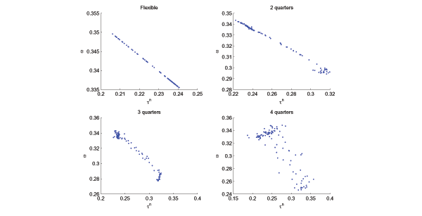
Figure 5. Dynamic relationship between worker's effective bargaining power (![]() ) and ex-post inflation rate under the Ramsey policy for various degrees of nominal rage rigidity.
) and ex-post inflation rate under the Ramsey policy for various degrees of nominal rage rigidity.
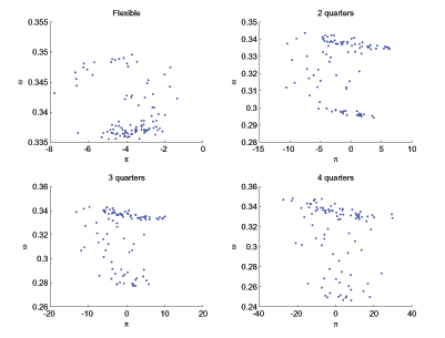
Figure 6. Simulation of the labor tax rate and real government debt obligations in flexible-wage model.
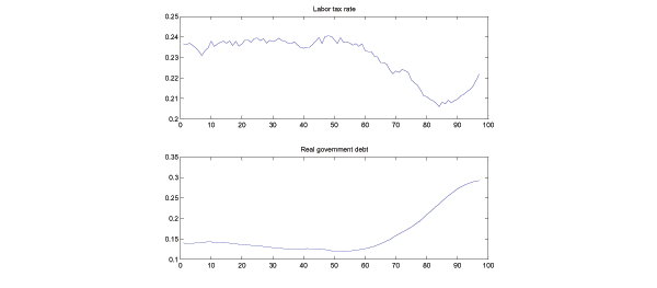
Figure 7. Realizations of inflation and unemployment rate under the Ramsey policy for various degrees of nominal wage rigidity.
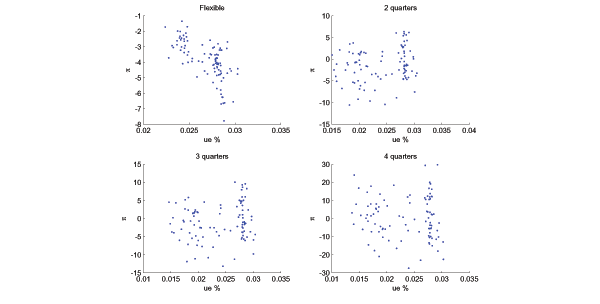
Figure 8. In model with bargaining over hours, key steady-state Ramsey allocation and policy variables as a function of nominal wage adjustment cost parameter ![]() .
. ![]() and
and![]() expressed in annualized percentage points.
expressed in annualized percentage points.
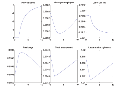
Figure 9. In RTM model, key steady-state Ramsey allocation and policy variables as a function of nominal wage adjustment cost parameter ![]() .
. ![]() and
and![]() expressed in annualized percentage points.
expressed in annualized percentage points.
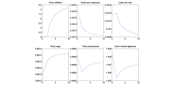
Figure 10. In RTW model, key steady-state Ramsey allocation and policy variables as a function of nominal wage adjustment cost parameter ![]() .
. ![]() and
and ![]() expressed in annualized percentage points.
expressed in annualized percentage points.
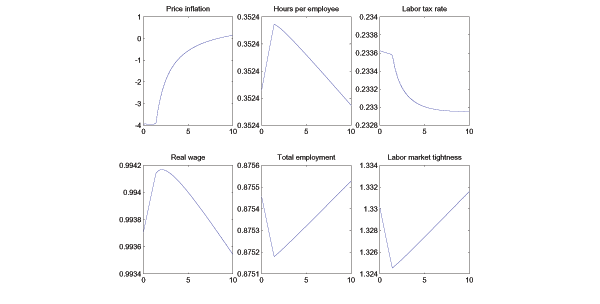
Table 3 (Panel 1). Flexible Wages
| Variable | Mean | Std. Dev. | Auto corr. | Corr | Corr | Corr |
|---|---|---|---|---|---|---|
| 0.2359 | 0.0842 | 0.9909 | -0.6654 | -0.0718 | 0.2613 | |
| -3.1063 | 13.8521 | 0.9802 | -0.0041 | -0.0043 | -0.1088 | |
| -3.3516 | 11.3765 | 0.9806 | 0.2866 | 0.2139 | -0.1353 | |
| 0.3726 | 0.1945 | 0.9879 | -0.0073 | 0.0123 | -0.1295 | |
| 0.4196 | 0.0108 | 0.9484 | 1.0000 | 0.7299 | -0.0970 | |
| 0.9951 | 0.0208 | 0.9729 | 0.6661 | 0.5077 | 0.0233 | |
| 0.3502 | 0.0056 | 0.9886 | 0.6331 | 0.0218 | -0.1539 | |
| 0.8749 | 0.0051 | 0.9828 | -0.3742 | 0.2369 | 0.1470 | |
| 0.1646 | 0.0015 | 0.7707 | 0.2606 | 0.1245 | 0.0445 | |
| 1.3178 | 0.0526 | 0.9802 | -0.3210 | 0.2743 | 0.1595 | |
| 0.1378 | 0.2007 | 0.9906 | 0.5226 | 0.0819 | -0.1113 | |
| 0.3372 | 0.0493 | 0.9909 | 0.6654 | 0.0718 | -0.2613 |
Simulation-based moments in the model with Nash bargaining over hours and heterogeneity between workers and non-workers driving processes are ![]() and
and ![]() .
.
![]() ,
, ![]() , and
, and ![]() reported in
annualized percentage points.
reported in
annualized percentage points.
Table 3 (Panel 2). Two Quarters of Nominal Wage Stickiness
| Variable | Mean | Std. Dev. | Auto corr. | Corr | Corr | Corr |
|---|---|---|---|---|---|---|
| 0.2362 | 0.0548 | 0.9968 | -0.3653 | 0.1634 | 0.2396 | |
| -2.7976 | 6.2892 | 0.2819 | -0.5021 | -0.4350 | 0.0946 | |
| -3.0089 | 2.6568 | 0.9583 | -0.0397 | 0.0883 | -0.1960 | |
| 1.2392 | 0.5276 | 0.9201 | -0.1949 | -0.1605 | -0.4909 | |
| 0.4194 | 0.0080 | 0.9149 | 1.0000 | 0.7957 | -0.1071 | |
| 0.9956 | 0.0176 | 0.6627 | 0.8254 | 0.7973 | -0.2941 | |
| 0.3501 | 0.0037 | 0.9933 | 0.3052 | -0.2309 | -0.0773 | |
| 0.8746 | 0.0037 | 0.9805 | 0.0654 | 0.5593 | 0.0210 | |
| 0.1643 | 0.0010 | 0.5798 | 0.2783 | 0.2645 | 0.0459 | |
| 1.3116 | 0.0373 | 0.9756 | 0.1401 | 0.6419 | 0.0294 | |
| 0.1362 | 0.2228 | 0.9974 | 0.1566 | -0.0995 | 0.1557 | |
| 0.3380 | 0.0320 | 0.9774 | 0.3829 | -0.1368 | -0.2618 |
Simulation-based moments in the model with Nash bargaining over hours and heterogeneity between workers and non-workers driving processes are ![]() and
and ![]() .
.
![]() ,
, ![]() , and
, and ![]() reported in
annualized percentage points.
reported in
annualized percentage points.
Table 3 (Panel 3). Three Quarters of Nominal Wage Stickiness
| Variable | Mean | Std. Dev. | Auto corr. | Corr | Corr | Corr |
|---|---|---|---|---|---|---|
| 0.2359 | 0.0536 | 0.9972 | -0.3968 | 0.1245 | 0.2748 | |
| -0.2907 | 8.6085 | 0.0746 | -0.4541 | -0.4373 | 0.2061 | |
| -0.6727 | 1.7862 | 0.9387 | -0.1458 | -0.0654 | -0.2067 | |
| 3.6750 | 0.5879 | 0.8707 | -0.0899 | -0.1396 | -0.6049 | |
| 0.4194 | 0.0082 | 0.9255 | 1.0000 | 0.7999 | -0.1290 | |
| 0.9954 | 0.0245 | 0.5586 | 0.7111 | 0.6830 | -0.3922 | |
| 0.3501 | 0.0036 | 0.9922 | 0.3315 | -0.1972 | -0.1029 | |
| 0.8747 | 0.0033 | 0.9806 | 0.0999 | 0.5655 | 0.0000 | |
| 0.1645 | 0.0009 | 0.6757 | 0.2939 | 0.2799 | 0.0474 | |
| 1.3139 | 0.0338 | 0.9771 | 0.1701 | 0.6519 | 0.0084 | |
| 0.1430 | 0.3022 | 0.9980 | 0.1308 | 0.0253 | 0.2324 | |
| 0.3378 | 0.0321 | 0.9440 | 0.4409 | -0.0496 | -0.3183 |
Simulation-based moments in the model with Nash bargaining over hours and heterogeneity between workers and non-workers driving processes are ![]() and
and ![]() .
.
![]() ,
, ![]() , and
, and ![]() reported in
annualized percentage points.
reported in
annualized percentage points.
Table 3 (Panel 4). Four Quarters of Nominal Wage Stickiness
| Variable | Mean | Std. Dev. | Auto corr. | Corr | Corr | Corr |
|---|---|---|---|---|---|---|
| 0.2358 | 0.0571 | 0.9970 | -0.4675 | 0.0811 | 0.3028 | |
| 0.3880 | 10.6319 | 0.0252 | -0.4009 | -0.3980 | 0.2239 | |
| -0.1625 | 1.7287 | 0.9441 | -0.2274 | -0.1193 | -0.1847 | |
| 4.2816 | 0.6724 | 0.8514 | -0.0249 | -0.0874 | -0.6216 | |
| 0.4195 | 0.0086 | 0.9352 | 1.0000 | 0.7783 | -0.1560 | |
| 0.9951 | 0.0296 | 0.5097 | 0.6389 | 0.6244 | -0.4067 | |
| 0.3501 | 0.0038 | 0.9907 | 0.4031 | -0.1535 | -0.1403 | |
| 0.8748 | 0.0032 | 0.9804 | 0.0662 | 0.5425 | -0.0098 | |
| 0.1646 | 0.0009 | 0.7399 | 0.2544 | 0.2740 | 0.0472 | |
| 1.3162 | 0.0324 | 0.9778 | 0.1265 | 0.6268 | -0.0021 | |
| 0.1449 | 0.3579 | 0.9982 | 0.1261 | 0.0543 | 0.2490 | |
| 0.3374 | 0.0351 | 0.9249 | 0.5156 | 0.0199 | -0.3363 |
Simulation-based moments in the model with Nash bargaining over hours and heterogeneity between workers and non-workers driving processes are ![]() and
and ![]() .
.
![]() ,
, ![]() , and
, and ![]() reported in
annualized percentage points.
reported in
annualized percentage points.
Table 4 (Panel 1). Flexible Wages
| Variable | Mean | Std. Dev. | Auto corr. | Corr | Corr | Corr |
|---|---|---|---|---|---|---|
| 0.2422 | 0.0678 | 0.9899 | -0.6929 | -0.0425 | 0.2944 | |
| -3.5022 | 9.6131 | 0.9771 | 0.0437 | -0.0073 | -0.1298 | |
| -3.5096 | 9.6361 | 0.9748 | 0.1576 | 0.2063 | -0.1229 | |
| 1.4390 | 1.1351 | 0.9883 | 0.0502 | 0.0145 | -0.1633 | |
| 0.4237 | 0.0117 | 0.9546 | 1.0000 | 0.6903 | -0.1350 | |
| 0.9612 | 0.0089 | 0.9061 | 0.3933 | 0.9202 | 0.0458 | |
| 0.3474 | 0.0039 | 0.9846 | 0.6263 | -0.0457 | -0.1625 | |
| 0.8884 | 0.0043 | 0.9790 | 0.9341 | 0.5305 | -0.2421 | |
| 0.1824 | 0.0015 | 0.6131 | -0.0249 | 0.1318 | -0.0654 | |
| 1.6373 | 0.0598 | 0.9769 | 0.9788 | 0.5941 | -0.2693 | |
| 0.1387 | 0.1465 | 0.9900 | 0.4291 | 0.0529 | -0.0960 | |
| 0.2866 | 0.0117 | 0.9823 | 0.3739 | -0.2991 | -0.3548 |
Simulation-based moments in the right-to-manage model with
heterogeneity between workers and non-workers; driving processes
are ![]() and
and ![]() .
. ![]() ,
, ![]() , and
, and ![]() reported in
annualized percentage points. Asterisk denotes zero-lower-bound is
violated during simulations.
reported in
annualized percentage points. Asterisk denotes zero-lower-bound is
violated during simulations.
Table 4 (Panel 2). Two Quarters of Nominal Wage Stickiness
| Variable | Mean | Std. Dev. | Auto corr. | Corr | Corr | Corr |
|---|---|---|---|---|---|---|
| 0.2440 | 0.0620 | 0.9968 | -0.5056 | 0.2801 | -0.0381 | |
| -3.6109 | 3.4865 | 0.8307 | -0.4485 | -0.5538 | -0.1654 | |
| -3.6053 | 2.8654 | 0.9975 | -0.2081 | 0.0493 | -0.2575 | |
| 0.4503 | 0.3678 | 0.9787 | -0.3443 | -0.4322 | -0.2699 | |
| 0.4234 | 0.0091 | 0.9361 | 1.0000 | 0.5863 | 0.0814 | |
| 0.9613 | 0.0099 | 0.9192 | 0.3465 | 0.9496 | -0.0531 | |
| 0.3472 | 0.0040 | 0.9918 | 0.4374 | -0.3548 | 0.1741 | |
| 0.8882 | 0.0029 | 0.9631 | 0.9009 | 0.5630 | -0.0656 | |
| 0.1824 | 0.0013 | 0.4311 | 0.0828 | 0.1210 | -0.0613 | |
| 1.6336 | 0.0399 | 0.9583 | 0.9729 | 0.6330 | -0.0853 | |
| 0.1376 | 0.2992 | 0.9980 | 0.3757 | -0.0488 | 0.2126 | |
| 0.2865 | 0.0147 | 0.9868 | 0.2106 | -0.5627 | -0.0281 |
Simulation-based moments in the right-to-manage model with
heterogeneity between workers and non-workers; driving processes
are ![]() and
and ![]() .
. ![]() ,
, ![]() , and
, and ![]() reported in
annualized percentage points. Asterisk denotes zero-lower-bound is
violated during simulations.
reported in
annualized percentage points. Asterisk denotes zero-lower-bound is
violated during simulations.
Table 4 (Panel 3). Three Quarters of Nominal Wage Stickiness
| Variable | Mean | Std. Dev. | Auto corr. | Corr | Corr | Corr |
|---|---|---|---|---|---|---|
| 0.2412 | 0.0446 | 0.9960 | -0.3394 | 0.2686 | -0.1081 | |
| -1.3764 | 2.7970 | 0.7703 | -0.6099 | -0.8176 | -0.0179 | |
| -1.4067 | 1.4120 | 0.9984 | -0.2283 | -0.1435 | -0.1412 | |
| 2.7258 | 0.2818 | 0.9665 | -0.4980 | -0.7025 | -0.1449 | |
| 0.4237 | 0.0082 | 0.9234 | 1.0000 | 0.7510 | 0.1398 | |
| 0.9612 | 0.0094 | 0.9127 | 0.5825 | 0.9680 | -0.0742 | |
| 0.3473 | 0.0030 | 0.9877 | 0.2551 | -0.3571 | 0.2844 | |
| 0.8884 | 0.0026 | 0.9553 | 0.8707 | 0.7342 | -0.0509 | |
| 0.1825 | 0.0013 | 0.4137 | 0.1120 | 0.0914 | -0.0257 | |
| 1.6362 | 0.0365 | 0.9496 | 0.9604 | 0.8112 | -0.0634 | |
| 0.1682 | 0.4185 | 0.9990 | 0.3403 | 0.1754 | 0.1242 | |
| 0.2870 | 0.0115 | 0.9813 | -0.0498 | -0.6206 | 0.0189 |
Simulation-based moments in the right-to-manage model with
heterogeneity between workers and non-workers; driving processes
are ![]() and
and ![]() .
. ![]() ,
, ![]() , and
, and ![]() reported in
annualized percentage points. Asterisk denotes zero-lower-bound is
violated during simulations.
reported in
annualized percentage points. Asterisk denotes zero-lower-bound is
violated during simulations.
Table 4 (Panel 4). Four Quarters of Nominal Wage Stickiness
| Variable | Mean | Std. Dev. | Auto corr. | Corr | Corr | Corr |
|---|---|---|---|---|---|---|
| 0.2396 | 0.0408 | 0.9956 | -0.3500 | 0.2001 | -0.1094 | |
| -0.8514 | 2.5151 | 0.7361 | -0.7239 | -0.8777 | 0.0171 | |
| -0.9008 | 1.0222 | 0.9985 | -0.3316 | -0.1598 | -0.1137 | |
| 3.2653 | 0.2474 | 0.9595 | -0.6179 | -0.7644 | -0.1241 | |
| 0.4239 | 0.0084 | 0.9280 | 1.0000 | 0.7973 | 0.1336 | |
| 0.9612 | 0.0091 | 0.9087 | 0.6420 | 0.9697 | -0.0775 | |
| 0.3474 | 0.0027 | 0.9867 | 0.2507 | -0.3057 | 0.3035 | |
| 0.8884 | 0.0027 | 0.9577 | 0.8758 | 0.7699 | -0.0585 | |
| 0.1825 | 0.0013 | 0.4148 | 0.0979 | 0.0844 | -0.0173 | |
| 1.6372 | 0.0377 | 0.9523 | 0.9614 | 0.8469 | -0.0689 | |
| 0.1831 | 0.5530 | 0.9993 | 0.4373 | 0.2154 | 0.0811 | |
| 0.2874 | 0.0108 | 0.9805 | -0.0558 | -0.5705 | 0.0169 |
Simulation-based moments in the right-to-manage model with
heterogeneity between workers and non-workers; driving processes
are ![]() and
and ![]() .
. ![]() ,
, ![]() , and
, and ![]() reported in
annualized percentage points. Asterisk denotes zero-lower-bound is
violated during simulations.
reported in
annualized percentage points. Asterisk denotes zero-lower-bound is
violated during simulations.
Table 5 (Panel 1). Flexible Wages
| Variable | Mean | Std. Dev. | Auto corr. | Corr | Corr | Corr |
|---|---|---|---|---|---|---|
| 0.2348 | 0.0742 | 0.9928 | -0.6559 | -0.0845 | 0.2429 | |
| -3.4824 | 13.3103 | 0.9818 | -0.1041 | 0.0216 | -0.0917 | |
| -3.4406 | 11.3883 | 0.9830 | 0.1537 | 0.2447 | -0.1073 | |
| 0.4124 | 0.2392 | 0.9872 | -0.0919 | 0.0433 | -0.1091 | |
| 0.4217 | 0.0113 | 0.9501 | 1.0000 | 0.7174 | -0.0581 | |
| 0.9936 | 0.0170 | 0.9644 | 0.7727 | 0.5972 | 0.0242 | |
| 0.3523 | 0.0056 | 0.9907 | 0.6559 | 0.0463 | -0.1147 | |
| 0.8755 | 0.0044 | 0.9828 | -0.2951 | 0.2648 | 0.1192 | |
| 0.1654 | 0.0012 | 0.7193 | 0.3475 | 0.1308 | 0.0385 | |
| 1.3306 | 0.0465 | 0.9798 | -0.2232 | 0.3064 | 0.1290 | |
| 0.1388 | 0.2086 | 0.9927 | 0.5955 | 0.0712 | -0.1001 | |
| 0.3358 | 0.0425 | 0.9928 | 0.6488 | 0.0825 | -0.2470 |
Simulation-based moments in the right-to-work model with
heterogeneity between workers and non-workers; driving processes
are ![]() and
and ![]() .
. ![]() ,
, ![]() , and
, and ![]() reported in
annualized percentage points. Asterisk denotes zero-lower-bound is
violated during simulations.
reported in
annualized percentage points. Asterisk denotes zero-lower-bound is
violated during simulations.
Table 5 (Panel 2). Two Quarters of Nominal Wage Stickiness
| Variable | Mean | Std. Dev. | Auto corr. | Corr | Corr | Corr |
|---|---|---|---|---|---|---|
| 0.2349 | 0.0441 | 0.9885 | -0.2549 | 0.2366 | 0.1353 | |
| -2.4350 | 5.1105 | 0.3241 | -0.5324 | -0.4708 | 0.0151 | |
| -2.5646 | 2.4221 | 0.9282 | -0.0571 | 0.0753 | -0.2243 | |
| 1.6443 | 0.4616 | 0.9250 | -0.3023 | -0.2639 | -0.4851 | |
| 0.4215 | 0.0080 | 0.9079 | 1.0000 | 0.8240 | -0.0568 | |
| 0.9939 | 0.0140 | 0.7003 | 0.8639 | 0.8760 | -0.2104 | |
| 0.3523 | 0.0033 | 0.9915 | 0.2768 | -0.2186 | 0.0070 | |
| 0.8752 | 0.0033 | 0.9750 | 0.2165 | 0.6460 | -0.0556 | |
| 0.1652 | 0.0010 | 0.4874 | 0.3156 | 0.2496 | 0.0212 | |
| 1.3254 | 0.0335 | 0.9677 | 0.3063 | 0.7389 | -0.0548 | |
| 0.1383 | 0.2039 | 0.9975 | 0.1430 | -0.1026 | 0.2124 | |
| 0.3366 | 0.0251 | 0.9935 | 0.2668 | -0.2219 | -0.1651 |
Simulation-based moments in the right-to-work model with
heterogeneity between workers and non-workers; driving processes
are ![]() and
and ![]() .
. ![]() ,
, ![]() , and
, and ![]() reported in
annualized percentage points. Asterisk denotes zero-lower-bound is
violated during simulations.
reported in
annualized percentage points. Asterisk denotes zero-lower-bound is
violated during simulations.
Table 5 (Panel 3). Three Quarters of Nominal Wage Stickiness
| Variable | Mean | Std. Dev. | Auto corr. | Corr | Corr | Corr |
|---|---|---|---|---|---|---|
| 0.2347 | 0.0814 | 0.8599 | -0.5712 | 0.0392 | 0.1725 | |
| 0.2225 | 18.9486 | -0.0839 | -0.2659 | -0.2276 | 0.1763 | |
| -0.2737 | 3.1364 | 0.7279 | -0.1806 | -0.0704 | -0.1779 | |
| 4.9116 | 1.5836 | 0.8636 | 0.0888 | -0.0062 | -0.5927 | |
| 0.4215 | 0.0119 | 0.9413 | 1.0000 | 0.6837 | -0.2241 | |
| 0.9935 | 0.0457 | 0.3539 | 0.4677 | 0.4088 | -0.3858 | |
| 0.3523 | 0.0060 | 0.9929 | 0.6821 | 0.0481 | -0.2261 | |
| 0.8754 | 0.0039 | 0.9712 | -0.1723 | 0.4284 | -0.0005 | |
| 0.1653 | 0.0013 | 0.7043 | 0.1801 | 0.1898 | 0.0592 | |
| 1.3286 | 0.0400 | 0.9669 | -0.1281 | 0.4966 | 0.0117 | |
| 0.1420 | 0.4470 | 0.9973 | 0.1279 | 0.0178 | 0.2905 | |
| 0.3360 | 0.0455 | 0.9572 | 0.6779 | 0.0587 | -0.2975 |
Simulation-based moments in the right-to-work model with
heterogeneity between workers and non-workers; driving processes
are ![]() and
and ![]() .
. ![]() ,
, ![]() , and
, and ![]() reported in
annualized percentage points. Asterisk denotes zero-lower-bound is
violated during simulations.
reported in
annualized percentage points. Asterisk denotes zero-lower-bound is
violated during simulations.
A Nash Bargaining Over Wages
Here we derive the Nash-bargaining solution between an
individual worker and the firm in the model without an intensive
margin. For notational simplicity, we omit the conditional
expectations operator ![]() where it is understood.
Individuals' and firms' asset values are defined in nominal terms.
The marginal (nominal) value to the household of an individual who
works is
where it is understood.
Individuals' and firms' asset values are defined in nominal terms.
The marginal (nominal) value to the household of an individual who
works is
![\begin{displaymath} \mathbf{W_t} = (1-\tau^n_t)W_t \bar{h} - \frac{P_t A \bar{h}}{u_{2t}} + \beta E_t \left[\left(\frac{u_{2t+1}}{u_{2t}}\right) \left(\frac{P_t}{P_{t+1}}\right) \left( (1-\rho^x) \mathbf{W_{t+1}} + \rho^x \mathbf{U_{t+1}} \right) \right]. \end{displaymath}](img629.gif)
The marginal (nominal) value to the household of an individual who is unemployed and searching is
![\begin{displaymath} \mathbf{U_t} = \frac{P_t v}{u_{2t}} + \beta E_t \left[ \left(\frac{u_{2t+1}}{u_{2t}}\right) \left(\frac{P_t}{P_{t+1}}\right) \left( \theta_t k^f(\theta_t) (1-\rho^x) \mathbf{W_{t+1}} + (1-\theta_t k^f(\theta_t) (1-\rho^x) ) \mathbf{U_{t+1}} \right) \right]. \end{displaymath}](img630.gif)
Note that because these asset values are defined as nominal, the
nominal discount factor, which involves ![]() ,
appears. The value to an intermediate goods producer of a filled
job is
,
appears. The value to an intermediate goods producer of a filled
job is
![\begin{displaymath} \mathbf{J_t} = P_t z_t f(\bar{h}) - W_t h_t - \frac{\psi}{\upsilon}\left(\frac{W_t}{W_{t-1} \pi_t^{\chi}}-1\right)^{\upsilon} P_t + \beta E_t \left[ \left(\frac{u_{2t+1}}{u_{2t}}\right) \left(\frac{P_t}{P_{t+1}}\right) (1-\rho^x) \mathbf{J_{t+1}} \right], \end{displaymath}](img632.gif)
where
![]() is a Rotemberg-type resource cost of nominal wage adjustment. This
is the way in which we model nominal rigidity in the wage
bargaining process. The typical Rotemberg quadratic specification
sets
is a Rotemberg-type resource cost of nominal wage adjustment. This
is the way in which we model nominal rigidity in the wage
bargaining process. The typical Rotemberg quadratic specification
sets ![]() .
.
Bargaining occurs every period over ![]() . The firm
and worker maximize the Nash product
. The firm
and worker maximize the Nash product
| (43) |
where
![]() is the fixed weight given to
the worker's individual surplus. The first-order condition of the
Nash product with respect to
is the fixed weight given to
the worker's individual surplus. The first-order condition of the
Nash product with respect to ![]() is
is
| (44) |
We have
![]() ,
,
![]() , and
, and
![\begin{displaymath} \frac{\partial \mathbf{J_t}}{\partial W_t} = -\bar{h} - \psi \left(\frac{\pi^w_t}{\pi_t^{\chi}} - 1\right)^{\upsilon-1} \frac{\pi_t^{1-\chi}}{w_{t-1}} + \psi(1-\rho^x) \beta E_t \left[\frac{u_{2t+1}}{u_{2t}}\frac{P_t}{P_{t+1}} \left(\frac{\pi^w_{t+1}}{\pi_{t+1}^{\chi}}-1\right)^{\upsilon-1} \pi^w_{t+1} \frac{\pi_{t+1}^{1-\chi}}{w_t} \right]. \end{displaymath}](img642.gif)
|
(45) |
In computing the latter, we defined
![]() as the gross rate
of nominal wage inflation between
as the gross rate
of nominal wage inflation between ![]() and
and
![]() and of course had to take into account
that
and of course had to take into account
that ![]() affects
affects
![]() through the adjustment cost
function. A wage Phillips Curve is essentially subsumed inside
through the adjustment cost
function. A wage Phillips Curve is essentially subsumed inside
![]() .
.
Define
| (46) |
| (47) |
and
|
(48) |
The latter means
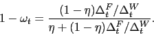
|
(49) |
With these definitions, we can write the Nash sharing rule as
| (50) |
which is a generalization of the usual Nash sharing rule.
Using the Bellman equation for the value of a match along with
the job-creation condition,
![]() . Using this as well as the values
. Using this as well as the values ![]() and
and ![]() , we can, after some tedious
algebra, express the outcome of the Nash bargain as
, we can, after some tedious
algebra, express the outcome of the Nash bargain as
![\begin{eqnarray*} \lefteqn{ \frac{\omega_t}{1-\omega_t} \left[ P_t z_t f(\bar{h}) - W_t \bar{h} - \frac{\psi}{\upsilon}\left(\frac{\pi^w_t}{\pi_t^{\chi}}-1\right)^{\upsilon}P_t + \frac{P_t \gamma}{k^f(\theta_t)}\right] = } \ \tiny & & (1-\tau^n_t) W_t \bar{h} - \frac{P_t A \bar{h}}{u_{2t}} - \frac{P_t v}{u_{2t}} \\ & & + (1-\theta_t k^f(\theta_t)) \beta E_t\left[\left(\frac{\omega_{t+1}}{1-\omega_{t+1}}\right) \left(\frac{u_{2t+1}}{u_{2t}}\right) \left(\frac{P_t}{P_{t+1}}\right) (1-\rho^x) \left[P_{t+1} z_{t+1} f(\bar{h}) - W_{t+1} \bar{h} - \frac{\psi}{\upsilon} \left(\frac{\pi^w_{t+1}}{\pi_{t+1}^{\chi}} - 1\right)^{\upsilon} P_{t+1} + \frac{P_{t+1} \gamma}{k^f(\theta_{t+1})} \right] \right]. \end{eqnarray*}](img657.gif)
Next, divide through by ![]() and define the real wage
as
and define the real wage
as
![]() to write the outcome of
bargaining as
to write the outcome of
bargaining as
![\begin{eqnarray*} \lefteqn{ \frac{\omega_t}{1-\omega_t} \left[ z_t f(\bar{h}) - w_t \bar{h} - \frac{\psi}{\upsilon}\left(\frac{\pi^w_t}{\pi_t^{\chi}}-1\right)^{\upsilon} + \frac{\gamma}{k^f(\theta_t)}\right] = } \\ & & (1-\tau^n_t) w_t \bar{h} - \frac{ A \bar{h}}{u_{2t}} - \frac{v}{u_{2t}} \\ & & + (1-\theta_t k^f(\theta_t)) \beta E_t\left[\left(\frac{\omega_{t+1}}{1-\omega_{t+1}}\right) \left(\frac{u_{2t+1}}{u_{2t}}\right) (1-\rho^x) \left[z_{t+1} f(\bar{h}) - w_{t+1} \bar{h} - \frac{\psi}{\upsilon}\left(\frac{\pi^w_{t+1}}{\pi_{t+1}^{\chi}}-1\right)^{\upsilon} + \frac{\gamma}{k^f(\theta_{t+1})} \right] \right], \end{eqnarray*}](img660.gif)
which is expression (22) in the text.
Note that if ![]() , then
, then
![]() , hence
, hence
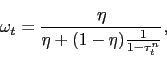
|
(51) |
so that it is only fluctuations in the labor tax rate that drive
fluctuations between ![]() and
and ![]() .
.
B Hours Determination
Here, we describe the details behind the three alternative
protocols we consider for hours determination. The Bellman
equations describing the value of a given state for an individual
worker, an unemployed individual, and a filled job are,
respectively:
![\begin{displaymath} \mathbf{W_t} = (1-\tau^n_t) W_t h_t - \frac{P_t e(h_t)}{u_{2t}} + \beta E_t \left[\left(\frac{u_{2t+1}}{u_{2t}}\right) \left(\frac{P_t}{P_{t+1}}\right) \left( (1-\rho^x) \mathbf{W_{t+1}} + \rho^x \mathbf{U_{t+1}} \right) \right], \end{displaymath}](img666.gif)
|
(52) |
![\begin{displaymath} \mathbf{U_t} = \frac{P_t v}{u_{2t}} + \beta E_t \left[ \left(\frac{u_{2t+1}}{u_{2t}}\right) \left(\frac{P_t}{P_{t+1}}\right) \left( \theta_t k^f(\theta_t) (1-\rho^x) \mathbf{W_{t+1}} + (1-\theta_t k^f(\theta_t) (1-\rho^x) ) \mathbf{U_{t+1}} \right) \right], \end{displaymath}](img667.gif)
|
(53) |
![\begin{displaymath} \mathbf{J_t} = P_t z_t f(h_t) - W_t h_t - \frac{\psi}{\upsilon}\left(\frac{W_t}{W_{t-1} \pi_t^{\chi}} - 1\right)^{\upsilon} + \beta E_t \left[ \left(\frac{u_{2t+1}}{u_{2t}}\right) \left(\frac{P_t}{P_{t+1}}\right) (1-\rho^x) \mathbf{J_{t+1}} \right]. \end{displaymath}](img668.gif)
|
(54) |
The difference between the protocols comes down to differences in the effective bargaining powers wielded by workers and firms: in each case, hours are determined by
![\begin{displaymath} \frac{\varrho_t}{1-\varrho_t} \mathbf{J_t} = (1-\tau^n_t) w_t h_t - \frac{e(h_t)}{u_{2t}} - \frac{v}{u_{2t}} + (1-\theta_t k^f(\theta_t))\beta E_t \left[\left(\frac{\varrho_{t+1}}{1-\varrho_{t+1}}\right) \left(\frac{u_{2t+1}}{u_{2t}}\right) (1-\rho_x) \mathbf{J_{t+1}} \right]. \end{displaymath}](img669.gif)
|
(55) |
The difference between the models amounts to differences in the
specification of the weight ![]()
B.1 Nash Bargaining Over Hours
If the parties bargain simultaneously over the nominal wage and
hours worked -- i.e., they maximize the Nash product
![]() with respect to both
with respect to both ![]() and
and ![]() -- the wage payment is still described by (22) (with appropriate replacement
of
-- the wage payment is still described by (22) (with appropriate replacement
of ![]() by
by ![]() ).
Defining
).
Defining
| (56) |
| (57) |
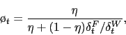
|
(58) |
the solution for hours is given by
![\begin{eqnarray*} \lefteqn{ \frac{\o_t}{1-\o_t} \left[ z_t f(h_t) - w_t h_t - \frac{\psi}{\upsilon}\left(\frac{\pi^w_t}{\pi_t^{\chi}}-1\right)^{\upsilon} + \frac{\gamma}{k^f(\theta_t)}\right] = } \\ & & (1-\tau^n_t) w_t h_t - \frac{e(h_t)}{u_{2t}} - \frac{v}{u_{2t}} \\ & & + (1-\theta_t k^f(\theta_t)) \beta E_t\left[\left(\frac{\o_{t+1}}{1-\o_{t+1}}\right) \left(\frac{u_{2t+1}}{u_{2t}}\right) (1-\rho^x) \left[z_{t+1} f(h_{t+1}) - w_{t+1} h_{t+1} - \frac{\psi}{\upsilon}\left(\frac{\pi^w_{t+1}}{\pi_{t+1}^{\chi}}-1\right)^{\upsilon} + \frac{\gamma}{k^f(\theta_{t+1})} \right] \right], \end{eqnarray*}](img679.gif)
in which we have substituted the equilibrium value of ![]() using the job-creation condition:
using the job-creation condition:
![]() . This sharing rule is different from the wage-setting rule only in
that the worker's effective bargaining power in hours determination
is
. This sharing rule is different from the wage-setting rule only in
that the worker's effective bargaining power in hours determination
is ![]() rather than
rather than ![]() .
.
B.2 Right To Manage
In the right-to-manage (RTM) specification, the firm chooses
![]() to maximize
to maximize ![]() after wage negotiations are over. This second-stage optimization
yields
after wage negotiations are over. This second-stage optimization
yields
![]() , a standard condition from
a neoclassical labor market. Invert this expression to express
hours as a function of the nominal wage,
, a standard condition from
a neoclassical labor market. Invert this expression to express
hours as a function of the nominal wage,
![]() . Both the
worker and the firm take as given this function when bargaining
over the wage, hence we modify the Bellman equations:
. Both the
worker and the firm take as given this function when bargaining
over the wage, hence we modify the Bellman equations:
![\begin{displaymath} \mathbf{W_t} = (1-\tau^n_t) W_t h\left(\frac{W_t}{P_t}\right) - \frac{P_t e\left(h\left(\frac{W_t}{P_t}\right)\right)}{u_{2t}} + \beta E_t \left[\left(\frac{u_{2t+1}}{u_{2t}}\right) \left(\frac{P_t}{P_{t+1}}\right) \left( (1-\rho^x) \mathbf{W_{t+1}} + \rho^x \mathbf{U_{t+1}} \right) \right], \end{displaymath}](img688.gif)
|
(59) |
![\begin{displaymath} \mathbf{J_t} = P_t z_t f\left(h\left(\frac{W_t}{P_t}\right)\right) - W_t h\left(\frac{W_t}{P_t}\right) - \frac{\psi}{\upsilon}\left(\frac{W_t}{W_{t-1} \pi_t^{\chi}} - 1\right)^{\upsilon} + \beta E_t \left[ \left(\frac{u_{2t+1}}{u_{2t}}\right) \left(\frac{P_t}{P_{t+1}}\right) (1-\rho^x) \mathbf{J_{t+1}} \right]. \end{displaymath}](img689.gif)
|
(60) |
Taking into account the dependence of ![]() on
on
![]() , we can express the marginal values with
respect to the nominal wage
, we can express the marginal values with
respect to the nominal wage ![]() as
as
| (61) |
| (62) |
![\begin{displaymath} \Xi_t \equiv - \psi \left(\frac{\pi^w_t}{\pi_t^{\chi}} - 1\right)^{\upsilon-1} \frac{\pi_t^{1-\chi}}{w_{t-1}} + \psi(1-\rho^x) \beta E_t \left[\frac{u_{2t+1}}{u_{2t}}\frac{P_t}{P_{t+1}} \left(\frac{\pi^w_{t+1}}{\pi_{t+1}^{\chi}}-1\right)^{\upsilon-1} \pi^w_{t+1} \frac{\pi_{t+1}^{1-\chi}}{w_t} \right]. \end{displaymath}](img695.gif)
|
(63) |
The second equality above uses the fact that under RTM,
![]() . Defining
. Defining
![]() ,
,
![]() ,
and
,
and
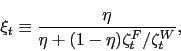
|
(64) |
the bargained wage is determined according to
![\begin{eqnarray*} \lefteqn{ \frac{\xi_t}{1-\xi_t} \left[ z_t f(h_t) - w_t h_t - \frac{\psi}{\upsilon}\left(\frac{\pi^w_t}{\pi_t^{\chi}}-1\right)^{\upsilon} + \frac{\gamma}{k^f(\theta_t)}\right] = } \\ & & (1-\tau^n_t) w_t \bar{h} - \frac{e(h_t)}{u_{2t}} - \frac{v}{u_{2t}} \\ & & + (1-\theta_t k^f(\theta_t)) \beta E_t\left[\left(\frac{\xi_{t+1}}{1-\xi_{t+1}}\right) \left(\frac{u_{2t+1}}{u_{2t}}\right) (1-\rho^x) \left[ z_{t+1} f(h_{t+1}) - w_{t+1} h_{t+1} - \frac{\psi}{\upsilon}\left(\frac{\pi^w_{t+1}}{\pi_{t+1}^{\chi}}-1\right)^{\upsilon} + \frac{\gamma}{k^f(\theta_{t+1})} \right] \right], \end{eqnarray*}](img700.gif)
in which ![]() is the relevant effective worker
bargaining power.
is the relevant effective worker
bargaining power.
B.3 Right To Work
An alternative to firms unilaterally choosing how many hours
their employees work is that workers choose their hours themselves.
The this right-to-work (RTW) specification, we assume that is the
the worker that chooses ![]() to maximize
to maximize ![]() after wage negotiations are over. This
second-stage optimization yields
after wage negotiations are over. This
second-stage optimization yields
![]() , also a standard
condition from a neoclassical labor market. Inverting this
expression to express hours as a function of the nominal wage gives
, also a standard
condition from a neoclassical labor market. Inverting this
expression to express hours as a function of the nominal wage gives
![]() . The
function
. The
function ![]() is distinct from the function
is distinct from the function
![]() from the RTM protocol. Both the worker and
the firm take as given
from the RTM protocol. Both the worker and
the firm take as given ![]() when bargaining over
the nominal wage. The Bellman equations under the RTW protocol are
thus
when bargaining over
the nominal wage. The Bellman equations under the RTW protocol are
thus
![\begin{displaymath} \mathbf{W_t} = (1-\tau^n_t) W_t \tilde{h}\left(\frac{W_t}{P_t}\right) - \frac{P_t e\left(\tilde{h}\left(\frac{W_t}{P_t}\right)\right)}{u_{2t}} + \beta E_t \left[\left(\frac{u_{2t+1}}{u_{2t}}\right) \left(\frac{P_t}{P_{t+1}}\right) \left( (1-\rho^x) \mathbf{W_{t+1}} + \rho^x \mathbf{U_{t+1}} \right) \right], \end{displaymath}](img709.gif)
|
(65) |
![\begin{displaymath} \mathbf{J_t} = P_t z_t f\left(\tilde{h}\left(\frac{W_t}{P_t}\right)\right) - W_t \tilde{h}\left(\frac{W_t}{P_t}\right) - \frac{\psi}{\upsilon}\left(\frac{W_t}{W_{t-1} \pi_t^{\chi}} - 1\right)^{\upsilon} + \beta E_t \left[ \left(\frac{u_{2t+1}}{u_{2t}}\right) \left(\frac{P_t}{P_{t+1}}\right) (1-\rho^x) \mathbf{J_{t+1}} \right]. \end{displaymath}](img710.gif)
|
(66) |
Taking into account the dependence of ![]() on
on
![]() , we can express the marginal values with
respect to the the nominal wage
, we can express the marginal values with
respect to the the nominal wage ![]() as
as
| (67) |
| (68) |
where, just as in the RTM model,
![\begin{displaymath} \Xi_t \equiv - \psi \left(\frac{\pi^w_t}{\pi_t^{\chi}} - 1\right)^{\upsilon-1} \frac{\pi_t^{1-\chi}}{w_{t-1}} + \psi(1-\rho^x) \beta E_t \left[\frac{u_{2t+1}}{u_{2t}}\frac{P_t}{P_{t+1}} \left(\frac{\pi^w_{t+1}}{\pi_{t+1}^{\chi}}-1\right)^{\upsilon-1} \pi^w_{t+1} \frac{\pi_{t+1}^{1-\chi}}{w_t} \right]. \end{displaymath}](img716.gif)
|
(69) |
The difference between the RTM and RTW models is that here we
cannot make the substitution
![]() whereas under the RTM
protocol we could. The definitions of
whereas under the RTM
protocol we could. The definitions of ![]() and
and
![]() are thus appropriately modified
compared to the RTM version, and the bargained wage payment is
determined according to this modified weight.
are thus appropriately modified
compared to the RTM version, and the bargained wage payment is
determined according to this modified weight.
References
Andolfatto, David/ 1996/ Business Cycles and Labor-Market Search/ American Economic Review/ 86/ 112-132.
Aiyagari, S. Rao, Albert Marcet, Thomas J, Sargent, and Juha Seppala/ 2002/ Optimal Taxation without State-Contingent Debt/ Journal of Political Economy/ 110/ 1220-1254.
Arseneau, David M. and Sanjay K. Chugh/ 2006/ Ramsey Meets Hosios: The Optimal Capital Tax and Labor Market Efficiency/ 870.
Aruoba, S. Boragan and Sanjay K. Chugh/ 2006/ Optimal Fiscal and Monetary Policy When Money is Essential/ 880.
Barro, Robert J/ 1977/ Long-Term Contracting, Sticky Prices, and Monetary Policy/ Journal of Monetary Economics/ 3/ 305-316.
Blanchard, Olivier and Peter Diamond/ 1989/ The Beveridge Curve/ Brookings Papers on Economic Activity/ 1/ 1-76.
Blanchard, Olivier and Jordi Gali/ 2006a/ Real Wage Rigidities and the New Keynesian Model/ Journal of Money, Credit, and Banking.
Blanchard, Olivier and Jordi Gali/ 2006b/ A New Keynesian Model with Unemployment/ MIT.
Chari, V.V., Lawrence Christiano, and Patrick Kehoe/ 1991/ Optimal Fiscal and Monetary Policy: Some Recent Results/ Journal of Money, Credit, and Banking/ 23/ 519-539.
Christoffel, Kai and Tobias Linzert/ 2005/ The Role of Real Wage Rigidity and Labor Market Frictions for Unemployment and Inflation Dynamics/ European Central Bank.
Chugh, Sanjay K/ 2006a/ Optimal Fiscal and Monetary Policy with Sticky Wages and Sticky Prices/ Review of Economic Dynamics/ 9/ 683-714.
Chugh, Sanjay K/ 2006b/ Optimal Inflation Persistence: Ramsey Taxation with Capital and Habits/ Journal of Monetary Economics.
Cooley, Thomas F. and Vincenzo Quadrini/ 2004/ Optimal Monetary Policy in a Phillips-Curve World/ Journal of Economic Theory/ 118/ 174-208.
Domeij, David/ 2005/ Optimal Capital Taxation and Labor Market Search/ Review of Economic Dynamics/ 8/ 623-650.
Erceg, Christoper J., Dale W. Henderson, and Andrew Levin/ 2000/ Optimal Monetary Policy with Staggered Wage and Price Contracts/ Journal of Monetary Economics/ 46/ 281-313.
Gertler, Mark and Antonella Trigari/ 2006/ Unemployment Fluctuations with Staggered Nash Bargaining/ New York University.
Goodfriend, Marvin and Robert G. King/ 2001/ The Case for Price Stability/ NBER Working Paper 8423.
Hagedorn, Marcus and Iourii Manovskii/ 2005/ The Cyclical Behavior of Equilibrium Unemployment and Vacancies Revisited/ University of Pennsylvania.
Hall, Robert E/ 2005/ Equilibrium Wage Stickiness/ American Economic Review/ 95/ 50-65.
Hosios, Arthur J/ 1990/ On the Efficiency of Matching and Related Models of Search and Unemployment/ Review of Economic Studies/ 57/ 279-298.
Krause, Michael U. and Thomas A. Lubik/ 2005/ The (Ir)relevance of Real Wage Rigidity in the New Keynesian Model with Search Frictions/ Journal of Monetary Economics.
Merz, Monika/ 1995/ Search in the Labor Market and the Real Business Cycle/ Journal of Monetary Economics/ 36/ 269-300.
Pissarides, Christopher A/ 2000/ Equilibrium Unemployment Theory/ MIT Press.
Schmitt-Grohe, Stephanie and Martin Uribe/ 2004a/ Optimal Fiscal and Monetary Policy Under Imperfect Competition/ Journal of Macroeconomics/ 26/ 183-209.
Schmitt-Grohe, Stephanie and Martin Uribe/ 2004b/ Optimal Fiscal and Monetary Policy Under Sticky Prices/ Journal of Economic Theory/ 114/ 198-230.
Schmitt-Grohe, Stephanie and Martin Uribe/ 2004c/ Solving Dynamic General Equilibrium Models Using a Second-Order Approximation to the Policy Function/ Journal of Economic Dynamics and Control/ 28/ 755-775.
Schmitt-Grohe, Stephanie and Martin Uribe/ 2006/ Comparing Two Variants of Calvo-Type Wage Stickiness/ Duke University.
Shimer, Robert/ 2005/ The Cyclical Behavior of Equilibrium Unemployment and Vacancies/ American Economic Review/ 95/ 25-49.
Siu, Henry E/ 2004/ Optimal Fiscal and Monetary Policy with Sticky Prices/ Journal of Monetary Economics/ 51/ 576-607.
Trigari, Antonella/ 2006/ The Role of Search Frictions and Bargaining for Inflation Dynamics/ Bocconi University.
Footnotes
1. The views expressed here are solely those of the authors and should not be interpreted as reflecting the views of the Board of Governors of the Federal Reserve System or of any other person associated with the Federal Reserve System. Return to text
2. Email address: [email protected]. Return to text
3. Email address: [email protected] Return to text
4. Thus, we follow Merz (1995), Andolfatto (1996), and much of the subsequent literature in this regard by assuming full consumption insurance between employed and unemployed individuals. Return to text
5. To understand this, note from the
household budget constraint that period-![]() profits are
received, in keeping with the usual timing of income receipts in a
cash/credit model, in period
profits are
received, in keeping with the usual timing of income receipts in a
cash/credit model, in period ![]() . The multiplier
associated with the period-
. The multiplier
associated with the period-![]() household flow
budget constraint is
household flow
budget constraint is
![]() . Hence, the derivative of the
Lagrangian of the household problem with respect to
. Hence, the derivative of the
Lagrangian of the household problem with respect to ![]() is
is
![]() . Return to text
. Return to text
6. Our notation surrounding the time-varying bargaining weights is adapted from Gertler and Trigari (2006). Return to text
7. Note, however, that because part of
output is absorbed by vacancy posting costs, ![]() does not correspond to labor's share of output;
nonetheless, we choose
does not correspond to labor's share of output;
nonetheless, we choose ![]() to remain as close
as possible to conventional models. Return to text
to remain as close
as possible to conventional models. Return to text
8. As we pointed out in Section 3, our dynamic solution method drops the ZLB constraint (30) and then checks whether the ZLB constraint is violated during simulated runs. Return to text
9. Both ![]() and
and
![]() were introduced in
Section 2.4. Return to text
were introduced in
Section 2.4. Return to text
10. Because, as shown in
Appendix A, ![]() . Return to
text
. Return to
text
11. Tax rate volatility does not arise because our overall model is excessively volatile: the coefficient of variation of total output is about 1.8 percent, in line with the data and with basic Ramsey models. Return to text
12. These standard deviations in percentage terms are simply equal to the raw standard deviations presented in Table 2 divided by the means. We could have equivalently computed the standard deviation of the logged variables. Return to text
13. And believe that most central bankers would call it volatile as well. Return to text
14. The basic intuition is that with incomplete markets, a one-time shock has (near-) permanent effects, hence the Ramsey government tries to insure the representative agent by maintaining at all times a very high asset position. Return to text
15. The reason for this is that with a
static departure from the Hosios parameterization, the underlying
model is already distorted; with ![]() too high, the
real wage is too low, and the Ramsey planner can indirectly
tip the bargaining balance back towards firm by taxing consumers
indirectly via inflation. Return to
text
too high, the
real wage is too low, and the Ramsey planner can indirectly
tip the bargaining balance back towards firm by taxing consumers
indirectly via inflation. Return to
text
16. A very similar issue arises in Cooley and Quadrini (2004). When studying the dynamics of their model, in order to ensure that the simulations are bounded away from the zero lower bound, they alter the Nash bargaining weight from the Hosios condition as well as introduce a second source of inefficiency. They report (p. 188), however, that the introduction of these features just induce a level shift of variables without altering the basic cyclical properties of the model; the same is true in our model. Return to text
17. An alternative approach to this issue has been to retain the Nash bargaining assumption but employ key parameter values that are quite different from those conventionally used in this class of models. A prominent example of this type of approach is Hagedorn and Manovskii (2006). Return to text
18. These relative volatilities are computed as a ratio of standard deviation percentages. Return to text
19. For the U.S. economy between 1964 and 2005, Gertler and Trigari (2006, p. 20) report relative standard deviations of unemployment of over 5, vacancies of over 6, and tightness of over 11. Return to text
20. Note that in the job-creation condition (19), it is the expected future real wage, not the contemporaneous real wage, that appears. Return to text
21. Another appropriate term may be right-to-shirk. Return to text
This version is optimized for use by screen readers. Descriptions for all mathematical expressions are provided in LaTex format. A printable pdf version is available. Return to text