
Board of Governors of the Federal Reserve System
International Finance Discussion Papers
Number 999, June 2010 --- Screen Reader
Version*
Monetary Policy and the Cyclicality of Risk1
NOTE: International Finance Discussion Papers are preliminary materials circulated to stimulate discussion and critical comment. References in publications to International Finance Discussion Papers (other than an acknowledgment that the writer has had access to unpublished material) should be cleared with the author or authors. Recent IFDPs are available on the Web at http://www.federalreserve.gov/pubs/ifdp/. This paper can be downloaded without charge from the Social Science Research Network electronic library at http://www.ssrn.com/.
Abstract:
We use a DSGE model that generates endogenous movements in risk premia to examine the positive and normative implications of alternative monetary policy rules. As emphasized by the microfinance literature, variation in risk arises because households face fixed costs of transferring cash across financial accounts, implying that some households rebalance their portfolios infrequently. We show that the model can account for the mean returns on equity and the risk-free rate, and in line with empirical evidence generates a decline in the equity premium following an unanticipated easing of monetary policy. An important result that emerges from our analysis is that countercyclical monetary policy generates higher average welfare than constant money growth or zero inflation policies.
Keywords: Limited financial market participation, equity premium, inflation targeting
JEL classification: E32, E44
1 Introduction
An important task in monetary economics is to identify simple and implementable rules that can help guide the conduct of monetary policy. To achieve this objective, researchers construct quantitative monetary models and use them as laboratories for evaluating alternative rules.3 Most models in this literature are variants of the workhorse New-Keynesian model with sticky prices. In these models, there is a limited role for monetary policy to influence the conditional variances of variables or the perceived riskiness of the economy, despite evidence to the contrary. This makes it difficult for these models to account for the finding that an important component through which monetary policy shocks affect stock prices occurs through changes in risk premia.4 Accordingly, a natural question to ask is whether the results that have emerged from this literature are robust to models in which endogenous movements in risk play a prominent role.
In this paper, we present a DSGE model in which asset and goods markets are segmented, because it is costly for households to transfer funds between these markets. Accordingly, households may only infrequently update their desired allocation of cash between a checking account devoted to purchasing goods and a brokerage account used for financial transactions. The optimal decision by an individual household to rebalance their cash holdings is a state-dependent one, reflecting that doing so involves paying a fixed cost in the presence of uncertainty. Households are heterogenous in this fixed cost, and only those households that rebalance their portfolios during the current period matter for determining asset prices. Because the fraction of these household changes over time in response to both real and monetary shocks, risk in the economy endogenously varies over time.5 We use this model to examine the positive and normative implications of several policy rules including inflation targeting rules, constant money growth rate rules, and rules that respond systematically to changes in aggregate activity.
There are a number of appealing features that make this framework well-suited for examining the effects of alternative policy rules. First, the model is able to account for the observed means on equity and risk-free rates with a power utility function with a reasonable degree of risk aversion. Second, in line with the evidence of [#!BK2005!#], the model generates a noticeable reduction in the equity premium in response to an unanticipated easing of monetary policy. Finally, recent microdata on household finance provides strong support for infrequent portfolio rebalancing.6
We find that the response of the equity premium to shocks depends critically on the systematic response of monetary policy. For inflation targeting rules or rules in which the monetary policy is procyclical, the equity premium moves countercyclically. However, for very aggressive countercyclical policies, the equity premium moves acyclically or even procyclically. A systematic change to monetary policy affects risk, because it influences a household's incentive to rebalance her portfolio, changing the behavior of households that matter for determining asset prices, and ultimately the amount of risk borne by these households. While systematic policy has an important influence on equity prices, monetary policy shocks, per se, account for only a small fraction of the average equity premium and the volatility of equity prices in the model.
An important result that emerges from our analysis is that countercyclical monetary policies imply aggregate welfare gains over inflation targeting or constant money growth rules. Countercyclical policy works well, because it improves the welfare of the majority of households, who tend to rebalance their portfolios infrequently. By transferring resources toward these households during booms, it allows them to raise their consumption without incurring the fixed costs associated with transferring funds across their brokerage and checking accounts. Thus, this policy effectively replicates how these households would respond, if they did not face these fixed costs.
The rest of this paper proceeds as follows. The next section describes the model. In Section 3 we use the model to explore some positive and normative effects of alternative monetary policy rules. We pay special attention to the effects of monetary policy on endogenous fluctuations in risk. Section 4 concludes.
2 The Model
The economy is populated by a large number of households, firms,
and a government sector. Trade occurs in financial and goods
markets in separate locations so that they are segmented from each
other. There are two sources of uncertainty in our economy --
aggregate shocks to technology, ![]() , and money
growth,
, and money
growth, ![]() . We let
. We let
![]() index the
aggregate event in period
index the
aggregate event in period ![]() with
with ![]() given, and
given, and
![]() denote the state,
which consists of the aggregate shocks that have occurred through
period
denote the state,
which consists of the aggregate shocks that have occurred through
period ![]() .
.
2.1 Firms
There is large number of perfectly competitive firms, which each
have access to the following technology for converting capital,
![]() , and labor,
, and labor, ![]() ,
into output,
,
into output, ![]() at dates
at dates ![]() :
:
| (1) |
The variable ![]() determines the economy's growth rate
and
determines the economy's growth rate
and ![]() is an aggregate technology shock
which follows a first-order autoregressive process:
is an aggregate technology shock
which follows a first-order autoregressive process:
| (2) |
where
![]() for all
for all
![]() .
.
Capital does not depreciate, and there exists no technology for
increasing or decreasing its magnitude. We adopt the normalization
that the aggregate stock of capital is equal to one. Labor is
supplied inelastically by households, and its supply is normalized
to one. Firm production begins at date 1. Following
Boldrin, Christiano, and Fisher (1997), we assume that firms have a one-period planning
horizon. To operate capital in period ![]() , a firm
must purchase it at the end of period
, a firm
must purchase it at the end of period ![]() from those
firms operating during period
from those
firms operating during period ![]() . To do so, a firm
issues equity, purchases capital, and hires workers.
. To do so, a firm
issues equity, purchases capital, and hires workers.
This problem implies that the equilibrium real wage,
![]() is given by:
is given by:
 |
(3) |
The return on capital or equity is given by:
![$\displaystyle 1+r^{e}(s^{t+1})= \frac{1+R^{e}(s^{t+1})}{\pi(s^{t+1})} =\frac{\left[\alpha \frac{Y(s^{t+1})}{K(s^{t})}+p_{k}(s^{t+1})\right]} {p_{k}(s^{t})}.$](img24.gif) |
(4) |
In the above,
![]() denotes the real price of capital and
denotes the real price of capital and
![]() is
the economy's inflation rate.
is
the economy's inflation rate.
2.2 Households
There are a large number of households of type ![]() , which denotes a household's fixed cost of making
state contingent transfers from a brokerage account to a checking
account. This cost is constant across time but differs across
household types according to the probability density function
, which denotes a household's fixed cost of making
state contingent transfers from a brokerage account to a checking
account. This cost is constant across time but differs across
household types according to the probability density function
![]() . We refer to a household that pays
her fixed cost as an active rebalancer and one that does not as
inactive.
. We refer to a household that pays
her fixed cost as an active rebalancer and one that does not as
inactive.
Brokerage Account. At date 0, a household learns her type and engages in an initial
round of trade in the asset market, as goods markets do not open
until date 1. With initial asset holdings,
![]() in her brokerage account
at date 0, the household purchases equity,
in her brokerage account
at date 0, the household purchases equity,
![]() , issued by the firms and a
complete set of one-period contingent claims,
, issued by the firms and a
complete set of one-period contingent claims,
![]() , issued by the government.
Accordingly, the flow of funds in a household's brokerage account
at date 0 is given by:
, issued by the government.
Accordingly, the flow of funds in a household's brokerage account
at date 0 is given by:
 |
(5) |
where ![]() is the price of the bond in state,
is the price of the bond in state,
![]() .
.
For dates ![]() , a household's brokerage account
evolves according to:
, a household's brokerage account
evolves according to:
 |
|||
| (6) |
where
![]() is a non-state contingent
transfer of funds from a household's brokerage account to checking
account at date
is a non-state contingent
transfer of funds from a household's brokerage account to checking
account at date ![]() chosen at date 0. A household can
alter this initial transfer plan by choosing
chosen at date 0. A household can
alter this initial transfer plan by choosing
![]() , which requires paying
the fixed cost
, which requires paying
the fixed cost ![]() . Accordingly,
. Accordingly,
![]() is an indicator variable equal
to one if a household opts to pay her fixed cost and make a
state-contingent transfer and equal to zero if a household does
not.7
is an indicator variable equal
to one if a household opts to pay her fixed cost and make a
state-contingent transfer and equal to zero if a household does
not.7
We view the fixed cost, ![]() , as reflecting
cognitive costs associated with collecting and processing
information necesssary to recompute the optimal portfolio
allocation in response to shocks.8 The key assumption we
make about a household's initial allocation scheme,
, as reflecting
cognitive costs associated with collecting and processing
information necesssary to recompute the optimal portfolio
allocation in response to shocks.8 The key assumption we
make about a household's initial allocation scheme,
![]() , is that it is non-state
contingent. By incorporating this initial portfolio decision and a
fixed cost of altering it in response to shocks, our model is
broadly consistent with the micro evidence that many households
adjust their portfolio decisions very infrequently.9
, is that it is non-state
contingent. By incorporating this initial portfolio decision and a
fixed cost of altering it in response to shocks, our model is
broadly consistent with the micro evidence that many households
adjust their portfolio decisions very infrequently.9
Checking Account. For ![]() , a household purchases goods for
consumption,
, a household purchases goods for
consumption,
![]() , and works in the labor
market. To purchase goods in period
, and works in the labor
market. To purchase goods in period ![]() , a household
uses cash in her checking account:
, a household
uses cash in her checking account:
| (7) |
At the beginning of period ![]() , a household has
, a household has
![]() dollars in her checking
account with which to purchase goods. A household also receives
cash from her non-state contingent transfer plan and
dollars in her checking
account with which to purchase goods. A household also receives
cash from her non-state contingent transfer plan and
![]() dollars from her
brokerage account, if she chooses to incur the fixed cost and
transfer additional funds.10
dollars from her
brokerage account, if she chooses to incur the fixed cost and
transfer additional funds.10
We have focused on transfers only between a checking account (i.e., more liquid assets) and a brokerage account (i.e., less liquid assets). In practice, a household has access to a wider range of financial products such as credit cards and other ''near-money'' assets that blur this distinction. In principle, one could incorporate such near-money assets by incorporating an additional account into the model whose assets can not directly be used to purchase goods but whose transaction cost is smaller than for the financial assets in the brokerage account. However, extending the model along these lines greatly complicates the analysis and we abstract from this possibility.
Each household inelastically supplies her labor to the economy's
firms. With a household's labor supply normalized to one, a
household earns real wage income, ![]() . This
wage income is received at the end of the period so it can not be
used for current consumption. Accordingly, a household cash in its
checking account at the end of period
. This
wage income is received at the end of the period so it can not be
used for current consumption. Accordingly, a household cash in its
checking account at the end of period ![]() is given
by:11
is given
by:11
| (8) |
A household's problem is to choose
![]() and
and
![]()
![]() to maximize:
to maximize:
 |
(9) |
subject to equations (5)-(8), taking prices
and initial holdings of money, bonds, and stocks as given. In
equation (9), the
function ![]() denotes the probability distribution
over history
denotes the probability distribution
over history ![]() .
.
2.3 Monetary Policy
The government issues the economy's one-period state-contingent
bonds and controls the economy's money stock, ![]() . Its budget constraints at date 0 is
. Its budget constraints at date 0 is
![]() where
where ![]() is given, and at dates
is given, and at dates ![]() , its budget constraint is:
, its budget constraint is:
 |
(10) |
with ![]() given. Monetary policy is
specified to follow a rule for money growth,
given. Monetary policy is
specified to follow a rule for money growth,
 ,
of the form:
,
of the form:
| (11) |
where
![]() for all
for all ![]() . This rule allows for a systematic
response of money to changes in technology (or equivalently output
given that capital and labor are fixed). When
. This rule allows for a systematic
response of money to changes in technology (or equivalently output
given that capital and labor are fixed). When
![]() , money growth is
procyclical, and when
, money growth is
procyclical, and when
![]() , money growth is
countercyclical. For our benchmark rule, we set
, money growth is
countercyclical. For our benchmark rule, we set
![]() .
.
The simple rules we evaluate include a constant money supply
rule in which
![]() , a
procyclical rule in which
, a
procyclical rule in which
![]() and
and
![]() , and a countercyclical
rule in which
, and a countercyclical
rule in which
![]() and
and
![]() . An additional rule that
we consider that is not nested by equation (11) is a zero
inflation or a price level targeting rule. This rule requires that
. An additional rule that
we consider that is not nested by equation (11) is a zero
inflation or a price level targeting rule. This rule requires that
![]() be chosen such that
be chosen such that
![]() for all
for all ![]() .
.
2.4 Equilibrium Characterization
The economy's resource constraint is:
![$\displaystyle Y(s^{t}) = \textrm{exp}( \theta_t + \eta t) =\int^{\infty}_{0} \left[ c(s^{t},\gamma )+\gamma z(s^{t},\gamma ) \right] f(\gamma)d\gamma,$](img85.gif) |
(12) |
as aggregate output is exogenous. The economy's price level and inflation rate can be obtained from:12
| (13) |
which imply that velocity is constant and inflation is given by:
| (14) |
The consumption of an inactive household (i.e., one that sets
![]() ) is given by:
) is given by:
 |
(15) |
From this expression, we can see that inflation is distortionary, since, all else equal, it reduces the consumption of inactive households. Accordingly, an unanticipated increase in money that raises inflation will induce the marginal household to pay her fixed cost and become active. Although the consumption of inactive households rises due to an increase in wages following an unexpected technological improvement, the benefits of being active are even greater, reflecting that active consumption is boosted by both higher wage and capital income. Thus, a technology shock will also boost the number of active households.
There is perfect risk-sharing amongst active households, and we
assume that the initial asset holdings,
![]() , of the households
implies:
, of the households
implies:
| (16) |
Accordingly, the consumption of active households is independent of
![]() . To further characterize, the
consumption of active and inactive households, we need to determine
. To further characterize, the
consumption of active and inactive households, we need to determine
![]() . A household's choice of
. A household's choice of
![]() satisfies:
satisfies:
)g(s^t)ds^t=0.$](img96.gif) |
(17) |
This latter condition implies that in states of the world in which
a household is inactive (i.e.,
![]() ), the household chooses
), the household chooses
![]() to equate her expected
discounted value of marginal utility of its consumption to the
expected discounted value of the marginal utility of consumption of
the active households. Accordingly, the non-state contingent
transfer plan provides some consumption insurance to households
with large fixed costs.
to equate her expected
discounted value of marginal utility of its consumption to the
expected discounted value of the marginal utility of consumption of
the active households. Accordingly, the non-state contingent
transfer plan provides some consumption insurance to households
with large fixed costs.
We now characterize a household's decision for
![]() given optimal decisions for
given optimal decisions for
![]() ,
,
![]() , and
, and
![]() . A household will choose to be
active if
. A household will choose to be
active if
![]() where
where
![]() is defined by:
is defined by:
| (18) |
and inactive otherwise. Equation (18) implies that
there is a marginal household with fixed cost
![]() whose net gain of
rebalancing is equal to the cost of transferring funds across the
two markets. The net gain,
whose net gain of
rebalancing is equal to the cost of transferring funds across the
two markets. The net gain,
![]() , is
simply the difference in the level of utility from being active as
opposed to inactive. The net cost of making the state-contingent
transfer comprises the fee
, is
simply the difference in the level of utility from being active as
opposed to inactive. The net cost of making the state-contingent
transfer comprises the fee ![]() and the
amount transferred by the household, since
and the
amount transferred by the household, since
![]() .
.
The asset pricing kernel in the economy depends on the consumption of the rebalancers and is given by:
![$\displaystyle m(s^{t+1}) = \beta \frac{U'[c_A(s^{t+1})]}{U'[c_A(s^{t})]}.$](img110.gif) |
(19) |
This pricing kernel is the state-contingent price of a security
expressed in consumption units and normalized by the probabilities
of the state. This pricing kernel can be used to determine the real
risk-free rate (![]() ) as well as the real return on
equity (
) as well as the real return on
equity (![]() ). These returns are given by:
). These returns are given by:
![$\displaystyle [1+r^f(s^t)]^{-1} = \int_{s_{t+1}} m(s^t,s_{t+1}) g(s_{t+1}\vert s^t) ds_{t+1},$](img113.gif) |
(20) |
![$\displaystyle 1 = \int_{s_{t+1}} m(s^t,s_{t+1}) [1+r^e(s^t,s_{t+1})] g(s_{t+1}\vert s^t)ds_{t+1},$](img114.gif) |
(21) |
where
![]() denotes the
probability of state
denotes the
probability of state ![]() conditional on state
conditional on state
![]() . Using these two equations, we can then
define the equity premium in our economy as:13
. Using these two equations, we can then
define the equity premium in our economy as:13
![$\displaystyle \frac{ \textrm{E}_t[1+r^e_{t+1}]}{1+r^f_t}= 1 - \textrm{cov}_t\left(m_{t+1},1+r^e_{t+1}\right).$](img119.gif) |
(22) |
3 Quantitative Analysis
In this section, we show that the model has reasonable asset pricing properties. We then use the model as a laboratory for evaluating the performance of alternative monetary policy rules. Before doing so, we briefly discuss the model's calibration and a deterministic version of the model.
3.1 Functional Forms and Calibration
Household's preferences are given by the isoelastic utility
function,
![]() , where
, where
![]() is the coefficient of relative risk
aversion. In this paper, we follow the discussion and the survey of
the literature in [#!Hall2008!#] and [#!Guvenen08!#], and set the
relative risk aversion coefficient equal to
is the coefficient of relative risk
aversion. In this paper, we follow the discussion and the survey of
the literature in [#!Hall2008!#] and [#!Guvenen08!#], and set the
relative risk aversion coefficient equal to ![]() .
Consistent with a quarterly model, we set
.
Consistent with a quarterly model, we set
![]() , implying the economy grows at
an annualized rate near 2%, and choose
, implying the economy grows at
an annualized rate near 2%, and choose
![]() . The economy's capital share,
. The economy's capital share,
![]() , is 0.36.
, is 0.36.
For the distribution of the fixed cost, ![]() , we assume that there is some small positive mass
of households with zero fixed costs and choose the remaining
distribution,
, we assume that there is some small positive mass
of households with zero fixed costs and choose the remaining
distribution, ![]() , to be log-normal so that
, to be log-normal so that
![]() . We set
. We set
![]() ,
,
![]() , and
, and
![]() , which imply that, on average,
about 6 percent of households rebalance their portfolios in a
quarter with some households rebalancing frequently and a large
mass of households rarely rebalancing. Such a calibration is
broadly in line with evidence that household portfolio allocation
displays substantial inertia.14
, which imply that, on average,
about 6 percent of households rebalance their portfolios in a
quarter with some households rebalancing frequently and a large
mass of households rarely rebalancing. Such a calibration is
broadly in line with evidence that household portfolio allocation
displays substantial inertia.14
For the monetary policy shock, we set
![]() ,
,
![]() and
and
![]() . This value for
. This value for
![]() is in line with the value used by
Alvarez, Atkeson, and Kehoe (2002). We set
is in line with the value used by
Alvarez, Atkeson, and Kehoe (2002). We set ![]() so that average,
annualized money growth rate is 2%. We calibrated the technology
shocks based on the time series properties of aggregate
consumption. We set
so that average,
annualized money growth rate is 2%. We calibrated the technology
shocks based on the time series properties of aggregate
consumption. We set
![]() and chose
and chose
![]() so that the standard
deviation for annualized consumption growth is 3 percent,
consistent with annual data on U.S. consumption from 1889-2009. As
discussed in the appendix, the model is solved numerically using a
global algorithm.
so that the standard
deviation for annualized consumption growth is 3 percent,
consistent with annual data on U.S. consumption from 1889-2009. As
discussed in the appendix, the model is solved numerically using a
global algorithm.
3.2 Non-Stochastic Steady State
In a deterministic environment, the model reduces to a
representative agent economy. According to equation (17), a household
that chooses to be inactive obtains the same level of consumption
as an active household. An inactive household can obtain such a
level of consumption by choosing her initial plan such that
![]() ,
where
,
where ![]() takes on the same value across all
inactive households and the tildes over the variables reflect that
these variables have been detrended by
takes on the same value across all
inactive households and the tildes over the variables reflect that
these variables have been detrended by
![]() . With consumption the same
across households, all households with
. With consumption the same
across households, all households with
![]() will never rebalance their
portfolios, and the households with
will never rebalance their
portfolios, and the households with
![]() will be indifferent between
rebalancing or using the non-state contingent transfer,
will be indifferent between
rebalancing or using the non-state contingent transfer, ![]() .
.
The non-stochastic steady state highlights the important role
that the initial transfer scheme plays in the model. Without this
plan, the model is similar to other models of endogenous
segmentation such as Alvarez, Atkeson, and Kehoe (2009), and in that case, the
consumption of active households exceeds the consumption of
inactive households, who would only receive
![]() . As
a result, an increase in steady-state inflation,
. As
a result, an increase in steady-state inflation, ![]() , would lower
, would lower
![]() and raise the number of active
households. In contrast, in our model, inactive households choose
and raise the number of active
households. In contrast, in our model, inactive households choose
![]() so that their consumption level
reflects not only the proceeds from working but the proceeds from
capital markets. An increase in
so that their consumption level
reflects not only the proceeds from working but the proceeds from
capital markets. An increase in ![]() induces inactive
households to choose a larger
induces inactive
households to choose a larger ![]() and the degree of
market segmentation remains unaffected: the inactive households are
still those with
and the degree of
market segmentation remains unaffected: the inactive households are
still those with
![]() .
.
3.3 Asset Pricing Implications
Table 1 displays
several statistics of interest from alternative versions of the
model and compares them with their empirical counterparts taken
from Guvenen (2009). As a reference point, the third column of the
table reports the results from the economy with a single
representative household.15 For our baseline calibration, with a
relatively low coefficient of relative risk aversion, as discussed
in Mehra and Prescott (1985), the representative agent model is unable to
replicate prominent asset pricing features: the average equity
premium is only 0.2% and the average (real) risk-free rate is 8.8%
on an annualized basis. As discussed in Weil (1989), it is
possible to match the observed equity premium in this model by
increasing ![]() ; however, this comes at the cost
of generating a counterfactual average risk-free rate.
; however, this comes at the cost
of generating a counterfactual average risk-free rate.
The fourth column of Table 1 shows the results from the benchmark calibration of the model with endogenous rebalancing. This model is consistent with the high average equity premium and the low and smooth risk-free rate observed in the data. The model's Sharpe ratio at 0.18 is below the point estimate based on U.S. data, reflecting that the volatility of excess stock returns exceeds that observed in the data. Still, the Sharpe ratio is much higher than in the representative agent economy and lies within the 95 percent confidence interval.
A key reason the model can generate a large average equity
premium with ![]() is that the volatility of
consumption of active households is higher than average consumption
volatility. As shown in Table 1, the volatility
of consumption growth for households is 5.6 times greater than for
average households. The consumption volatility of an active
household is higher than an inactive household, because the two
aggregate shocks only affect the consumption of the latter type of
household through changes in labor income. In contrast, active
households experience fluctuations in both labor and capital
income. A household that rebalances more frequently accepts this
higher consumption volatility in return for a higher average level
of consumption. This implication is in line with evidence of
Parker and Vissing-Jorgensen (2009) provided that 'high consumption' households are in
fact more likely to rebalance. In particular, these authors find
that the exposure to changes in aggregate consumption growth of
households in the top 10 percent of the consumption distribution is
about five times that of households in the bottom 80 percent.
is that the volatility of
consumption of active households is higher than average consumption
volatility. As shown in Table 1, the volatility
of consumption growth for households is 5.6 times greater than for
average households. The consumption volatility of an active
household is higher than an inactive household, because the two
aggregate shocks only affect the consumption of the latter type of
household through changes in labor income. In contrast, active
households experience fluctuations in both labor and capital
income. A household that rebalances more frequently accepts this
higher consumption volatility in return for a higher average level
of consumption. This implication is in line with evidence of
Parker and Vissing-Jorgensen (2009) provided that 'high consumption' households are in
fact more likely to rebalance. In particular, these authors find
that the exposure to changes in aggregate consumption growth of
households in the top 10 percent of the consumption distribution is
about five times that of households in the bottom 80 percent.
As shown in Table 1, the non-state
contingent plan plays a critical role in generating the average
equity premium. When the households do not have access to this plan
(i.e.,
![]() ), the asset pricing
implications are similar to those of the representative agent
model: the average equity premium is close to zero while the
average risk-free rate is above 8 percent. Without the financial
plan, the average fraction of rebalancers is 29 percent. Even if we
lower this average fraction to 6 percent by increasing the fixed
cost of rebalancing, the asset pricing implications remain largely
unchanged and the average cost of rebalancing is over 27 percent of
GDP. In comparison, the average cost of rebalancing in the
benchmark model with the financial plan is 0.2 percent of GDP.
), the asset pricing
implications are similar to those of the representative agent
model: the average equity premium is close to zero while the
average risk-free rate is above 8 percent. Without the financial
plan, the average fraction of rebalancers is 29 percent. Even if we
lower this average fraction to 6 percent by increasing the fixed
cost of rebalancing, the asset pricing implications remain largely
unchanged and the average cost of rebalancing is over 27 percent of
GDP. In comparison, the average cost of rebalancing in the
benchmark model with the financial plan is 0.2 percent of GDP.
The non-state contingent plan, by allowing inactive households
to receive proceeds from capital markets in states of the world in
which they do not rebalance, helps these households raise their
average level of consumption and smooth it. Higher values of
![]() , all else equal, tend to
reduce the consumption of active households and the incentive to
rebalance, while increasing the sensitivity of the consumption of
active households to technology and monetary shocks.16 This
increased sensitivity of the consumption of active households to
shocks raises the volatility of their consumption, helping induce a
relatively large average equity premium in the endogenous
rebalancing model.
, all else equal, tend to
reduce the consumption of active households and the incentive to
rebalance, while increasing the sensitivity of the consumption of
active households to technology and monetary shocks.16 This
increased sensitivity of the consumption of active households to
shocks raises the volatility of their consumption, helping induce a
relatively large average equity premium in the endogenous
rebalancing model.
The fifth column of Table 1 displays the results using the benchmark calibration of the endogenous rebalancing model except that there are no monetary shocks. The results in the table are very similar to the version of the model with monetary shocks, as the average equity premium, for instance, is 6.1% in the economy with both technology and monetary shocks and 5.8% in the economy with just technology shocks. Accordingly, monetary shocks only make a small contribution to asset pricing fluctuations in the model.
3.4 Monetary Policy Shocks and the Equity Premium
Besides having reasonable implications for the average risk premium and risk-free rate, the model generates a noticeable increase in the equity premium following a monetary contraction. This implication is in line with the evidence of Bernanke and Kuttner (2005), who find that a broad index of stock prices registers a gain of 1 percent in reaction to a 25 basis point easing of the federal funds rate. They decompose the response of stock prices into changes in current and expected future dividends, changes in current and expected future real interest rates, and changes in expected excess equity returns. They conclude that an important channel in which increases in stock prices occur is through changes in equity premia.
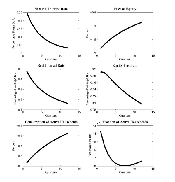
Figure 2 displays the impulse responses to an unanticipated decline in money growth in the endogenous rebalancing model.17 As in the limited participation models of Lucas (1990) and Fuerst (1992), the model displays a noticeable liquidity effect, with the nominal interest rate increasing 25 basis points in response to the monetary tightening. Moreover, as in Alvarez, Atkeson, and Kehoe (2002), the effect is persistent. Equity prices fall about 2 percent on impact, with part of the decline reflecting a higher equity premium. On impact, the equity premium rises about 20 basis points. Such a response is in line with the empirical evidence presented in Bernanke and Kuttner (2005).
To understand why the model generates a rise in the equity premium, the bottom left panel of Figure 2 shows the response of the consumption of households that actively rebalance. The monetary contraction has no effect on output but has an important redistributive effect. It raises the consumption of non-active households, whose real money balances available for consumption increase, and lowers the consumption of those that choose to rebalance. As shown in the bottom right panel, this redistribution induces a fall in the fraction of households that actively rebalance. Accordingly, there is a reduction in the degree of risk-sharing amongst active households, which helps drive up the equity premium.18
The model's ability to generate a liquidity effect and an increase in the equity premium after a monetary contraction is notable, especially when contrasted with New Keynesian models. These models as emphasized by Edge (2007) have difficulty producing a liquidity effect unless one incorporates additional real rigidities such as habit persistence in consumption and time to plan and build for investment projects. In addition, there is a limited role for monetary policy to influence conditional variances of variables in New Keynesian models, and, as a result, it difficult for these models to account for the evidence of Bernanke and Kuttner (2005) on how the equity premium responds to monetary policy shocks.
3.5 Alternative Monetary Policy Rules and the Equity Premium
Given that the model is capable of accounting for some prominent
empirical findings regarding interest rates and the equity premium,
it is natural to use it as a laboratory for evaluating alternative
policy rules. We begin by evaluating how changes in the systematic
or anticipated component of the monetary policy rule affects the
average equity premium and the risk free rate. In particular, we
examine how changes in the average money growth rate, ![]() , the persistence of the money growth,
, the persistence of the money growth,
![]() , and the response of money to
output,
, and the response of money to
output,
![]() affect these variables.
affect these variables.
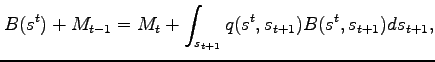
Figure 1 shows how changes in these parameters affect the average equity premium and risk-free rate. The figure also displays the sample averages for the risk-free rate and the equity premium (see the black dot labeled ''U.S. Data'') and the 5 confidence ellipse based on the estimates from Guvenen (2009). The points along the red line with diamonds represent different combinations of the mean equity premium and risk-free rate for money growth rates ranging from 0 to 10 percent on an annualized basis. For all the average money growth rates in this range, the model yields a mean equity premium and risk-free rate within the 95 confidence region. Moreover, changes in average inflation rate have relatively little effect on the average equity premium and real risk-free rate.
As indicated in our discussion of the non-stochastic steady
state, a higher average inflation rate increases the steady state
value of the households' initial plan. This same consideration
applies to the stochastic economy, as the function,
![]() , shifts up when
, shifts up when ![]() increases. As discussed above, an upward shift in
increases. As discussed above, an upward shift in
![]() increases the volatility of
active consumption and the average equity premium.19
increases the volatility of
active consumption and the average equity premium.19
The purple line with triangles in Figure 1 displays the
results from varying the persistence of the money growth process.
For values of
![]() between 0.2 and 0.95, the
combinations of mean equity premia and risk-free rates lie within
the 95 confidence region. Raising the persistence of money growth
shocks tends to reduce the average equity premium by driving up the
incentive for a household to rebalance her portfolio. This reflects
that a higher value of
between 0.2 and 0.95, the
combinations of mean equity premia and risk-free rates lie within
the 95 confidence region. Raising the persistence of money growth
shocks tends to reduce the average equity premium by driving up the
incentive for a household to rebalance her portfolio. This reflects
that a higher value of
![]() makes the monetary shocks both
larger and longer-lasting, benefitting active households. With more
households rebalancing, risk in financial markets is spread over
more households, active consumption growth becomes less volatile,
and its covariance with the return on equity diminishes.
Consequently, the average equity premium declines.20
makes the monetary shocks both
larger and longer-lasting, benefitting active households. With more
households rebalancing, risk in financial markets is spread over
more households, active consumption growth becomes less volatile,
and its covariance with the return on equity diminishes.
Consequently, the average equity premium declines.20
The green line with squares in Figure 1 shows the mean
of the equity premium and risk-free rate for different values of
![]() . A countercyclical monetary
policy rule (i.e.,
. A countercyclical monetary
policy rule (i.e.,
![]() ) tends to reduce the
average risk premium, while a procyclical rule tends to raise it.
Holding the fraction of rebalancers fixed, a procyclical
(countercyclical) rule tends to increase (decrease) the volatility
of consumption growth of active households, as a monetary injection
redistributes funds to active households during a boom when active
consumption is already high. Conversely, in a downturn, a
procyclical rule calls for lower money growth, redistributing cash
away from active households, which exacerbates the fall in the
consumption of active households.
) tends to reduce the
average risk premium, while a procyclical rule tends to raise it.
Holding the fraction of rebalancers fixed, a procyclical
(countercyclical) rule tends to increase (decrease) the volatility
of consumption growth of active households, as a monetary injection
redistributes funds to active households during a boom when active
consumption is already high. Conversely, in a downturn, a
procyclical rule calls for lower money growth, redistributing cash
away from active households, which exacerbates the fall in the
consumption of active households.
3.6 Monetary Policy and the Cyclicality of Risk
Before discussing the normative implications of alternative
policy rules, it is helpful to first examine how simple, systematic
rules alter the transmission of technology shocks and affect the
cyclicality of risk. Since our emphasis here is on systematic
component of monetary policy, we only consider rules in which
![]() . The
particular rules that we consider include a fixed money supply
rule, (
. The
particular rules that we consider include a fixed money supply
rule, (
![]() ), a procyclical rule
in which
), a procyclical rule
in which
![]() and
and ![]() , and a countercyclical rule in which
, and a countercyclical rule in which
![]() and
and ![]() . Finally, we consider a price level or zero inflation
targeting rule. From equation (14), this rule
implies that
. Finally, we consider a price level or zero inflation
targeting rule. From equation (14), this rule
implies that
![]() . Thus,
in order to keep inflation constant in response to a highly
persistent and positive technology shock, this rule will raise
monetary growth initially but contract it in future periods as the
shock gradually dies out.
. Thus,
in order to keep inflation constant in response to a highly
persistent and positive technology shock, this rule will raise
monetary growth initially but contract it in future periods as the
shock gradually dies out.
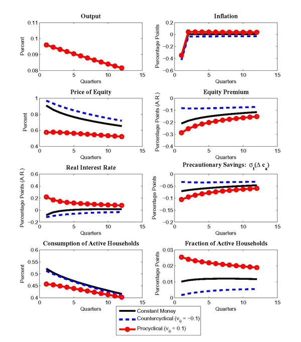
Figure 3 displays the response of the economy following a positive technology shock for the constant money supply rule, the countercyclical rule, and the procyclical rule. In each case, output is exogenous and rises about 0.1 percent on impact (top left panel of the Figure) after which it gradually returns to its pre-shocked level. A key result that emerges from Figure 3 is that the equity premium moves countercyclically under all three rules.
To understand this result, consider first the constant money supply rule (the solid black line). A positive technology shock raises the consumption of active rebalancers more than inactive households, since an active household changes her consumption in response to both the higher wage and capital income, while the consumption of inactive household responds only to the higher wage income. This jump in capital income induces more households to rebalance their cash allocation, which in turn helps lower risk in equity markets. Under the constant money growth rule, the equity premium falls about 20 basis points, which helps push up equity prices.
The real interest rate falls on impact, reflecting intertemporal smoothing motives by active households. However, the decline in real interest rates is small because of a reduction in precautionary savings by active households. This decline is evident in the fall in conditional volatility of consumption growth for active households (the middle right panel). Finally, inflation falls sharply under the constant money growth rule but quickly falls back to its pre-shocked level.
The procyclical rule (the red line with circles) has similar qualitative effects on the equity premium than the constant money supply rule though the effects are larger. By increasing the money growth rate when technology is high, monetary policy in effect transfers cash away from inactive households to active ones. Accordingly, there is a greater incentive to rebalance, and the fraction of rebalancers rises more, helping induce a larger fall in the equity premium than under the constant money supply rule. There is a larger decline in precautionary savings under the procyclical rule than the constant money supply rule. Accordingly, the real interest rate rises instead of falls in this case, leading to a smaller increase in equity prices than under a constant money rule. The countercyclical rule (blue dashed line) works in reverse relative to the procyclical rule. In this case, the response of the equity premium is smaller and the real rate falls by more, reflecting a smaller change in precautionary savings.
Figure 4 shows the effects of a more aggressive countercyclical rule (blue dashed line). In this case, the equity premium rises a bit after the technology shock and is essentially acyclical. This response reflects that monetary policy now vigorously counteracts the rise in the consumption of active rebalancers driven by the technology shock by redistributing funds away from active to inactive households, which spreads risk over a wider set of households. As shown in the top right panel of Figure 3, monetary policy achieves this redistribution by generating a persistent deflation.
Figure 4 also displays the case of a zero inflation targeting rule (red line with circles). The middle left panel shows that the real interest rate falls sharply under the zero inflation targeting rule, reflecting a large, temporary increase in money growth that is quickly reversed so that money growth becomes slightly negative in future periods. With the real interest rate falling sharply, the (real) price of equity jumps 2 percent and then declines to a level above its pre-shocked value.
The price of equity rises not only due to the fall in the real interest rate but also due to a sizeable decline in the equity premium. The equity premium moves countercyclically under a zero inflation targeting rule, because this rule calls for a large, temporary increase in the money growth rate after a positive technology shock. Consequently, there are increases in both the consumption of active households and the fraction of households that rebalance their portfolios. In addition, there is a reduction in precautionary savings by active households.
3.7 Welfare Implications of Alternative Monetary Policy Rules
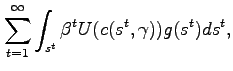
Table 2 compares aggregate welfare under alternative policy rules. We define aggregate welfare so that each household receives equal weight:
![$\displaystyle W(s_0) = \left[ \sum_{t=1}^{\infty }\int_{s^{t}}\int_{\gamma}\beta ^{t} U(c(s^{t},\gamma))g(s^{t})f(\gamma)d\gamma ds^t\right],$](img191.gif) |
(23) |
where ![]() is conditional on the initial state
of the world as well as the initial asset distribution. To compare
welfare across the different rules, we hold the initial asset
distribution,
is conditional on the initial state
of the world as well as the initial asset distribution. To compare
welfare across the different rules, we hold the initial asset
distribution, ![]()
![]() , fixed across policy rules.
To do so, we replace equation (16) with
, fixed across policy rules.
To do so, we replace equation (16) with
|
(24) |
and use the given initial asset distribution to determine a household's initial consumption.21
Table 2 provides a measure of the welfare gain in units of aggregate consumption by defining
![$\displaystyle \left[ \frac{W^{A}(s_0)-W^{B}(s_0)}{U'\left(C_s\right)C_s}\right],$](img198.gif)
where
![]() is welfare under fixed money
supply rule,
is welfare under fixed money
supply rule,
![]() denotes aggregate welfare under
an alternative monetary policy rule,
denotes aggregate welfare under
an alternative monetary policy rule, ![]() is the
level of aggregate consumption in nonstochastic steady state, and
is the
level of aggregate consumption in nonstochastic steady state, and
![]() is its associated
marginal utility. Accordingly, this index expresses the gain from
adopting a particular policy rule instead of the constant money
supply rule in terms of the permanent increase in steady state
consumption.
is its associated
marginal utility. Accordingly, this index expresses the gain from
adopting a particular policy rule instead of the constant money
supply rule in terms of the permanent increase in steady state
consumption.
From Table 2, it is clear
that the countercyclical rule with
![]() has the highest average
welfare, as it would raise the level of steady state consumption
about 0.25 percent relative to a fixed money supply rule. In
contrast, the procyclical rules perform poorly, resulting in either
a fall in welfare or only a small gain relative to the constant
money supply rule.
has the highest average
welfare, as it would raise the level of steady state consumption
about 0.25 percent relative to a fixed money supply rule. In
contrast, the procyclical rules perform poorly, resulting in either
a fall in welfare or only a small gain relative to the constant
money supply rule.
To understand these results better, Figure 5 displays the effects of alternative policy rules on the welfare of individual households. A common feature of all the policy rules is that welfare is decreasing in the fixed cost of households so that households in lower percentiles of the distribution rebalance more frequently and have greater welfare. This reflects that the consumption level of these households is higher albeit more volatile.
The top panel of Figure 5 shows the
welfare distribution for the fixed money supply rule (the solid
black line), the procyclical rule with
![]() (the red line with
circles), and the countercyclical rule with
(the red line with
circles), and the countercyclical rule with
![]() (the blue dashed line).
Relative to the fixed money supply rule, the countercyclical policy
improves the welfare of the majority of households, who are
primarily inactive, while modestly lowering the welfare of
households that frequently rebalance. This improved welfare of the
inactive types reflects that a countercyclical policy transfers
funds from active to inactive households in productive times,
allowing the inactive ones to raise their consumption without
incurring the fixed cost. Thus, this policy replicates what these
households would do if they did not face a fixed cost of
transferring funds from their brokerage account to their checking
account. In contrast, a procyclical policy enacts the reverse
redistribution plan: giving more funds to active households and
less to inactive ones during productive periods. While a small
fraction of very frequent rebalancers are better off under the
procyclical rule than the countercyclical rule, the majority of
households are worse off.
(the blue dashed line).
Relative to the fixed money supply rule, the countercyclical policy
improves the welfare of the majority of households, who are
primarily inactive, while modestly lowering the welfare of
households that frequently rebalance. This improved welfare of the
inactive types reflects that a countercyclical policy transfers
funds from active to inactive households in productive times,
allowing the inactive ones to raise their consumption without
incurring the fixed cost. Thus, this policy replicates what these
households would do if they did not face a fixed cost of
transferring funds from their brokerage account to their checking
account. In contrast, a procyclical policy enacts the reverse
redistribution plan: giving more funds to active households and
less to inactive ones during productive periods. While a small
fraction of very frequent rebalancers are better off under the
procyclical rule than the countercyclical rule, the majority of
households are worse off.
The bottom panel of Figure 5 compares the
zero inflation targeting rule (the magenta line with triangles) to
the fixed money supply rule and the countercyclical rule with
![]() . As shown in Table 2, a zero
inflation targeting rule improves the average welfare relative to a
constant money supply rule but performs worse than the
countercyclical rule with
. As shown in Table 2, a zero
inflation targeting rule improves the average welfare relative to a
constant money supply rule but performs worse than the
countercyclical rule with
![]() . The zero inflation
targeting rule raises welfare relative to the constant money growth
rule by sharply increasing the welfare of households that
frequently rebalance while only slightly reducing the welfare of
inactive households. Households that frequently rebalance are
better off, as the zero inflation targeting rule implies a large
transfer to active households in the initial period of a positive
shock. Still, for average welfare, the countercyclical rule with
. The zero inflation
targeting rule raises welfare relative to the constant money growth
rule by sharply increasing the welfare of households that
frequently rebalance while only slightly reducing the welfare of
inactive households. Households that frequently rebalance are
better off, as the zero inflation targeting rule implies a large
transfer to active households in the initial period of a positive
shock. Still, for average welfare, the countercyclical rule with
![]() outperforms the zero
inflation targeting rule and results in the highest average welfare
of the rules that we considered. As shown in Figure 5, this
countercyclical rule drives up the welfare of a large fraction of
households relative to either the constant money growth rule or the
zero inflation targeting rule and also tends to equalize welfare
across households.
outperforms the zero
inflation targeting rule and results in the highest average welfare
of the rules that we considered. As shown in Figure 5, this
countercyclical rule drives up the welfare of a large fraction of
households relative to either the constant money growth rule or the
zero inflation targeting rule and also tends to equalize welfare
across households.
4 Conclusions
We used a DSGE model that has reasonable implications for the equity premium and generates endogenous variations in risk to examine the positive and normative implications of alternative monetary policy rules. We showed that the response of the equity premium to shocks depends critically on the systematic response of monetary policy. Monetary policies primarily focused on inflation targeting induce procyclical movements in the equity premium, while very aggressive countercyclical policies induce acyclical movements. Countercyclical monetary policy can generate higher average welfare than constant money growth or inflation targeting rules by spreading consumption risk more broadly over households. A by-product of countercyclical policy is a sustained deflation, suggesting that the Friedman rule may also achieve superior outcomes. A natural extension of this paper is to compute optimal monetary policy and determine how well simple rules such as the Friedman rule or the countercyclical rule we emphasized here approximate it.
Appendix
In this appendix, we describe how the model is solved and how welfare is computed.
- Step 1: Solve the model under the fixed money supply rule using
equation (16), which
implies that active consumption is the same across households. To
do so, use quadrature to approximate the expectations associated
with the normally-distributed shocks (see Chapter 7 of
Judd (1999). We write equation (17) recursively,
and we choose
 such that the Euler error is
zero. To do so we apply the linear Fredholm integral equations
(Type 2), and use collocation to determine
such that the Euler error is
zero. To do so we apply the linear Fredholm integral equations
(Type 2), and use collocation to determine
 . See Section 10.8 in Judd's
book for a discussion of the linear Fredholm integral equations and
Chapter 11 for collocation. Specifically, we choose
. See Section 10.8 in Judd's
book for a discussion of the linear Fredholm integral equations and
Chapter 11 for collocation. Specifically, we choose
 such that the Euler errors
evaluated at the nonstochastic steady state value of technology are
equal to zero for a finite number of households. We then use
splines to approximate the function elsewhere. The other decision
rules (e.g., the ones for active consumption and
such that the Euler errors
evaluated at the nonstochastic steady state value of technology are
equal to zero for a finite number of households. We then use
splines to approximate the function elsewhere. The other decision
rules (e.g., the ones for active consumption and
 ) are chosen to satisfy
the model's other equilibrium conditions described in the
paper.
) are chosen to satisfy
the model's other equilibrium conditions described in the
paper. - Step 2: Use the solution from step 1 to compute welfare under the fixed money supply rule. To do so, we need to express average welfare recursively and again use quadrature, the linear Fredholm integral equations, and the decision rules determined in Step 1 to compute average welfare evaluated at the steady state level of technology.
- Step 3: Use the restrictions implied by equation (16) to determine
the initial asset position,
 , under the
fixed money supply rule. Use the sequence of asset market
constraints to write one intertemporal asset market constraint for
each household. See the appendix of Alvarez, Atkeson, and Kehoe (2002) for how to derive
this condition as well as the derivation of the equilibrium
conditions for a similar model. Equation (16) implies that
the value of the Lagrange multiplier,
, under the
fixed money supply rule. Use the sequence of asset market
constraints to write one intertemporal asset market constraint for
each household. See the appendix of Alvarez, Atkeson, and Kehoe (2002) for how to derive
this condition as well as the derivation of the equilibrium
conditions for a similar model. Equation (16) implies that
the value of the Lagrange multiplier,  , on
each agent's intertemporal asset market constraint is the same.
Using each of these constraints, the asset market clearing
condition, and taking the aggregate initial supply of bonds as
given, we can determine the multiplier
, on
each agent's intertemporal asset market constraint is the same.
Using each of these constraints, the asset market clearing
condition, and taking the aggregate initial supply of bonds as
given, we can determine the multiplier  and
and
 . Again, we use collocation to
approximate the function
. Again, we use collocation to
approximate the function  .
. - Step 4: Using
 from the fixed
money supply rule, solve the model under an alternative monetary
policy rule. To do so, we need to jointly solve for
from the fixed
money supply rule, solve the model under an alternative monetary
policy rule. To do so, we need to jointly solve for  and
and
 , the Lagrange multiplier on
a household's intertemporal asset market constraint, which
now differs across households. To solve for
, the Lagrange multiplier on
a household's intertemporal asset market constraint, which
now differs across households. To solve for
 , we use collocation applied
to the intertemporal asset market constraint of different
households. In doing so, we take into account that equation
(16) is no longer a
relevant equilibrium condition. Instead, when household
, we use collocation applied
to the intertemporal asset market constraint of different
households. In doing so, we take into account that equation
(16) is no longer a
relevant equilibrium condition. Instead, when household  chooses to be active, its consumption will be
proportional to the consumption of a household with zero fixed cost
(i.e.,
chooses to be active, its consumption will be
proportional to the consumption of a household with zero fixed cost
(i.e.,  ). This factor of proportionality
depends directly on
). This factor of proportionality
depends directly on
 and
and
 . The remaining equilibrium
conditions are modified to take this relationship into
account.
. The remaining equilibrium
conditions are modified to take this relationship into
account. - Step 5: Use the solution from step 4 to compute welfare under the alternative policy rule, which is done as described in step 2.
References
Alvarez, F., A. Atkeson, and P. Kehoe (2009). Time-Varying Risk, Interest Rates, and Exchange Rates in General Equilibrium. The Review of Economic Studies. forthcoming.
Alvarez, F., A. Atkeson, and P. J. Kehoe (2002). Money, Interest Rates, and Exchange Rates with Endogenously Segmented Markets. Journal of Political Economy 110, 73-112.
Ameriks, J. and S. P. Zeldes (2004). How Do Household Portfolio Shares Vary with Age? mimeo, Columbia University.
Ammer, J., C. Vega, and J. Wongswan (2008). Do Fundamentals Explain the International Impact of U.S. Interest Rates? Evidence at the Firm Level. International Finance Discussion Paper 2008-952 (October 2008).
Bacchetta, P. and E. van Wincoop (2009). Infrequent Portfolio Decisions: A Solution to the Forward Discount Puzzle. American Economic Review. Forthcoming.
Bernanke, B. and K. Kuttner (2005). What Explains the Stock Markets Reaction to Federal Reserve Policy? Journal of Finance LX, 1221-1257.
Bilias, Y., D. Georgarakos, and M. Haliassos (2008). Portfolio Inertia and Stock Market Fluctuations. CFS Working Paper 2006/4. Revised July 2008.
Boldrin, M., L. J. Christiano, and J. D. Fisher (1997). Habit Persistence and Asset Returns in an Exchange Economy. Macroeconomic Dynamics 1, 312-332.
Bonaparte, Y. and R. Cooper (2009). Costly Portfolio Adjustment. National Bureau of Economic Research Working Paper 15227.
Brunnermeier, M. and S. Nagel (2008). Do Wealth Fluctuations Generate Time-Varying Risk Aversion? Micro-Evidence from Individuals Asset Allocation. American Economic Review 98, 713-736.
Calvet, L. E., J. Y. Campbell, and P. Sodini (2009). Measuring the Financial Sophistication of Households. American Economic Review 99, 393-398.
Edge, R. M. (2007). Time-to-Build, Time-To-Plan, Habit Persistence, and the Liquidity Effect. Journal of Monetary Economics 54, 1644-1669.
Ehrmann, M. and M. Fratzscher (2004). Taking Stock: Monetary Policy Transmission to Equity Markets. Journal of Money, Credit and Banking 36, 719-737.
Fuerst, T. S. (1992). Liquidity, Loanable Funds, and Real Activity. Journal of Monetary Economics 29, 3-24.
Gabaix, X. and D. Laibson (2001). The 6D Bias and the Equity-Premium Puzzle. In B. Bernanke and J. Rotemberg (Eds.), NBER Macroeconomics Annual. MIT Press.
Gust, C. and D. López-Salido (2009a). Monetary Policy, Velocity, and the Equity Premium. Centre for Economic Policy Research Discussion Paper No. 7388.
Gust, C. and D. Lópezpez-Salido (2009b). Portfolio Inertia and the Equity Premium. International Finance Discussion Paper 984.
Guvenen, F. (2009). A Parsimonious Macroeconomic Model for Asset Pricing. Econometrica 77, 1711-1740.
Hall, R. E. (2009). Reconciling Cyclical Movements in the Marginal Value of Time and the Marginal Product of Labor. Journal of Political Economy 117, 281-323.
Hamilton, J. D. (1994). Time Series Analysis. Princeton, NJ: Princeton University Press.
Judd, K. L. (1999). Numerical Methods in Economics. Cambridge, MA: The MIT Press.
Khan, A. and J. K. Thomas (2007). Inflation and Interest Rates with Endogenous Market Segmentation. Federal Reserve Bank of Philadelphia Working Paper 07-1,.
Lucas, R. E. (1990). Liquidity and Interest Rates. Journal of Economic Theory 50, 237-264.
Mehra, R. and E. Prescott (1985). The Equity Premium Puzzle. Journal of Monetary Economics 15, 145-166.
Parker, J. and A. Vissing-Jorgensen (2009). Who Bears Aggregate Fluctuations and How? American Economic Review 99, 399-405.
Reis, R. (2006). Inattentive Consumers. Journal of Monetary Economics 53, 1761-1800.
Souleles, N. S. (2003). Household Portfolio Choice, Transactions Costs, and Hedging Motives. mimeo, University of Pennsylvania.
Taylor, J. B. (Ed.) (1999). Monetary Policy Rules. Chicago, IL: The University of Chicago Press.
Weil, P. (1989). The Equity Premium Puzzle and the Riskfree Rate Puzzle. Journal of Monetary Economics 24, 401-421.
Table 1. Unconditional Moments of Asset Returnsa
| Statistic | U.S. Data | Representative Agent | No Financial Plan | Benchmark Calibration | Technology Shocks Only |
|---|---|---|---|---|---|
| | 6.2 (2.0) | 0.2 | 0.2 | 6.1 | 5.8 |
| | 19.4 (1.4) | 7.8 | 7.9 | 33.6 | 32.2 |
| | 0.32 (0.1) | 0.04 | 0.03 | 0.18 | 0.18 |
1.9 (5.4) | 8.8 | 8.8 | 1.7 | 1.8 | |
| | 5.4 (0.6) | 1.1 | 1.0 | 4.2 | 3.8 |
| | 3.5 (0.4) | 3.2 | 3.3 | 3.0 | 3.0 |
| | 1 | 0.86 | 5.6 | 5.6 | |
| | 100 | 29 | 6 | 6 | |
| | 0 | 0.6 | 0.2 | 0.2 | |
| Avg. Cost of Reb. (% of GDP) | 0 | 21 | 0.2 | 0.2 |
![]() Results for the models based on population
moments.
Results for the models based on population
moments.
![]() The symbol
The symbol ![]() denotes the unconditional mean of a
variable and
denotes the unconditional mean of a
variable and ![]() denotes the standard deviation
of variable
denotes the standard deviation
of variable ![]() . Rates of
return are expressed in percent on an annualized basis.
. Rates of
return are expressed in percent on an annualized basis.
![]() This column
contains estimates (standard errors in parentheses) based on U.S.
data for the period 1890-1991 and are taken from
Guvenen (2008). The estimates for consumption are based on U.S.
data for the period 1889-2009 and are available online at /http://www.econ.yale.edu/~shiller/.
This column
contains estimates (standard errors in parentheses) based on U.S.
data for the period 1890-1991 and are taken from
Guvenen (2008). The estimates for consumption are based on U.S.
data for the period 1889-2009 and are available online at /http://www.econ.yale.edu/~shiller/.
Table 2. Welfare Implications of Alternative Monetary Policy Rules*
| Rule | Parameters: | Parameters: | Welfare Gain | Avg. Fraction of Rebalancers |
|---|---|---|---|---|
| Fixed Money Supply | 0 | 0 | 0.00 | 6.0 |
| Procyclical | 0 0 0 | 0.1 0.5 1 | -0.052 0.020 0.032 | 6.3 8.3 12.3 |
| Countercyclical | 0 0 0 | -0.1 -0.5 -1 | 0.053 0.258 -0.097 | 5.8 5.4 5.7 |
| Zero Inflation Target | - | - | 0.143 | 6.5 |
*With the exception of the zero inflation target, the monetary policy rule is given by:
where ![]() is the
economy's money growth rate,
is the
economy's money growth rate, ![]() is aggregate
output, and
is aggregate
output, and ![]() denotes the average money growth rate. Under the zero
inflation target,
denotes the average money growth rate. Under the zero
inflation target, ![]() is chosen so that
inflation is constant and equal to zero.
is chosen so that
inflation is constant and equal to zero.
Figure 1. Monetary Policy and the Average Equity Premium
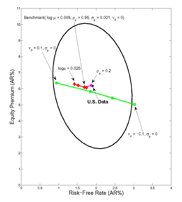
Note: The monetary policy rule is given by:
![]()
where ![]() is the
economy's money growth rate,
is the
economy's money growth rate, ![]() is aggregate
output,
is aggregate
output, ![]() denotes the average money growth rate,
and
denotes the average money growth rate,
and
![]() .
.
Figure 2. Impulse Response to a Contractionary Monetary Shock
(Deviation from Date 0 Expectation of a Variable)
Note: These impulse responses are from the benchmark calibration of the model with monetary policy specified as:
where ![]() is the
economy's money growth rate,
is the
economy's money growth rate, ![]() denotes the
average money growth rate,
denotes the
average money growth rate,
![]() ,
and
,
and
![]() .
.
Data for Figure 2
| Quarters | Nominal Interest Rate | Price of Equity | Real Interest Rate | Equity Premium | Consumption of Active Households | Fraction of Active Households |
|---|---|---|---|---|---|---|
| 1 | 0.24906 | -1.8308 | 0.47828 | 0.19128 | -0.56642 | -0.0037 |
| 2 | 0.19528 | -1.6842 | 0.41256 | 0.18984 | -0.52403 | -0.00545 |
| 3 | 0.15532 | -1.5577 | 0.36164 | 0.17924 | -0.48698 | -0.00654 |
| 4 | 0.12507 | -1.4469 | 0.32107 | 0.16742 | -0.45416 | -0.00723 |
| 5 | 0.10192 | -1.3482 | 0.28813 | 0.15606 | -0.42469 | -0.00764 |
| 6 | 0.083947 | -1.2594 | 0.26085 | 0.14549 | -0.39797 | -0.00787 |
| 7 | 0.069724 | -1.1788 | 0.23779 | 0.13579 | -0.37356 | -0.00796 |
| 8 | 0.058346 | -1.1051 | 0.21802 | 0.1269 | -0.35111 | -0.00795 |
| 9 | 0.049271 | -1.0374 | 0.20096 | 0.11864 | -0.33039 | -0.00787 |
| 10 | 0.042072 | -0.97499 | 0.18618 | 0.11087 | -0.31118 | -0.00774 |
| 11 | 0.036319 | -0.91719 | 0.17323 | 0.10358 | -0.29332 | -0.00757 |
| 12 | 0.031626 | -0.86355 | 0.16171 | 0.096774 | -0.27668 | -0.00737 |
Figure 3. Impulse Response to a Technology Shock for Alternative Policy Rules
(Deviation from Date 0 Expectation of a Variable)
Note: With the exception of the zero inflation target, the monetary policy rule is given by:
where ![]() is the
economy's money growth rate,
is the
economy's money growth rate, ![]() is aggregate
output, and
is aggregate
output, and ![]() denotes the average money growth
rate. Under the zero inflation target,
denotes the average money growth
rate. Under the zero inflation target, ![]() is
chosen so that inflation is constant and equal to
zero.
is
chosen so that inflation is constant and equal to
zero.
Data for Figure 3
| Quarters | Output: Red | Output: Black | Inflation: Blue | Inflation: Red | Price of Equity: Black | Price of Equity: Blue | Price of Equity: Red | Equity Premium: Black | Equity Premium: Blue | Equity Premium: Red | Real Interest Rate: Black | Real Interest Rate: Blue | Real Interest Rate: Red | Precautionary Savings: Black | Precautionary Savings: Blue | Precautionary Savings: Red | Consumption of Active Households: Black | Consumption of Active Households: Blue | Consumption of Active Households: Red | Fraction of Active Households: Black | Fraction of Active Households: Blue | Fraction of Active Households: Red |
|---|---|---|---|---|---|---|---|---|---|---|---|---|---|---|---|---|---|---|---|---|---|---|
| 1 | 0.096 | -0.384 | -0.4224 | -0.3456 | 0.90845 | 0.97314 | 0.5742 | -0.21012 | -0.08334 | -0.28706 | -0.08321 | -0.11692 | 0.21832 | -0.07118 | -0.0329 | -0.10609 | 0.52151 | 0.51162 | 0.45736 | 0.010152 | 0.001736 | 0.025446 |
| 2 | 0.094589 | 0.005645 | -0.03219 | 0.04348 | 0.85701 | 0.93734 | 0.57636 | -0.18731 | -0.08563 | -0.25332 | -0.03706 | -0.09792 | 0.16902 | -0.06689 | -0.03426 | -0.09527 | 0.50464 | 0.49888 | 0.45402 | 0.010982 | 0.002633 | 0.024094 |
| 3 | 0.093198 | 0.005562 | -0.03172 | 0.042841 | 0.81989 | 0.90559 | 0.573 | -0.1721 | -0.08572 | -0.23101 | -0.01542 | -0.0825 | 0.14431 | -0.06355 | -0.03483 | -0.08792 | 0.49142 | 0.48722 | 0.4493 | 0.011445 | 0.003314 | 0.023199 |
| 4 | 0.091828 | 0.00548 | -0.03125 | 0.042211 | 0.79049 | 0.87743 | 0.56796 | -0.1607 | -0.08485 | -0.21455 | -0.00325 | -0.07063 | 0.12879 | -0.06074 | -0.03495 | -0.08233 | 0.48019 | 0.47652 | 0.44419 | 0.01172 | 0.003838 | 0.022504 |
| 5 | 0.090478 | 0.0054 | -0.03079 | 0.041591 | 0.76596 | 0.85218 | 0.56233 | -0.15168 | -0.08355 | -0.20172 | 0.004158 | -0.06145 | 0.11772 | -0.05833 | -0.03482 | -0.07784 | 0.47023 | 0.46662 | 0.43896 | 0.011879 | 0.004248 | 0.021919 |
| 6 | 0.089148 | 0.00532 | -0.03034 | 0.04098 | 0.74474 | 0.82928 | 0.55649 | -0.14424 | -0.08204 | -0.1913 | 0.008853 | -0.05428 | 0.10913 | -0.05619 | -0.03453 | -0.0741 | 0.46116 | 0.45735 | 0.4337 | 0.011962 | 0.004571 | 0.021401 |
| 7 | 0.087838 | 0.005242 | -0.02989 | 0.040377 | 0.72594 | 0.80829 | 0.55058 | -0.13793 | -0.08044 | -0.18258 | 0.011866 | -0.04859 | 0.10208 | -0.05428 | -0.03414 | -0.0709 | 0.45274 | 0.44862 | 0.42845 | 0.011992 | 0.004828 | 0.020929 |
| 8 | 0.086547 | 0.005165 | -0.02945 | 0.039784 | 0.70894 | 0.78886 | 0.54464 | -0.13246 | -0.0788 | -0.17509 | 0.013822 | -0.04402 | 0.096113 | -0.05254 | -0.03369 | -0.0681 | 0.44483 | 0.44032 | 0.42323 | 0.011981 | 0.005032 | 0.020489 |
| 9 | 0.085274 | 0.005089 | -0.02902 | 0.039199 | 0.69335 | 0.77075 | 0.53869 | -0.1276 | -0.07717 | -0.16848 | 0.015041 | -0.0403 | 0.090885 | -0.05095 | -0.0332 | -0.0656 | 0.4373 | 0.4324 | 0.41803 | 0.011941 | 0.005194 | 0.020072 |
| 10 | 0.084021 | 0.005014 | -0.02859 | 0.038623 | 0.67888 | 0.75374 | 0.53274 | -0.12319 | -0.07555 | -0.16253 | 0.015681 | -0.03725 | 0.086147 | -0.04948 | -0.03268 | -0.06336 | 0.43011 | 0.4248 | 0.41286 | 0.011877 | 0.005321 | 0.019675 |
| 11 | 0.082786 | 0.00494 | -0.02817 | 0.038055 | 0.66533 | 0.73768 | 0.52679 | -0.11917 | -0.07395 | -0.15715 | 0.015911 | -0.03472 | 0.081818 | -0.04811 | -0.03215 | -0.06131 | 0.42318 | 0.41749 | 0.40772 | 0.011794 | 0.005419 | 0.019292 |
| 12 | 0.081569 | 0.004868 | -0.02776 | 0.037495 | 0.65254 | 0.72244 | 0.52084 | -0.11551 | -0.07239 | -0.15225 | 0.015894 | -0.0326 | 0.077874 | -0.04681 | -0.03161 | -0.05941 | 0.41647 | 0.41042 | 0.40261 | 0.011696 | 0.005493 | 0.018923 |
Figure 4. Impulse Response to a Technology Shock for a Zero Inflation Target
(Deviation from Date 0 Expectation of a Variable)
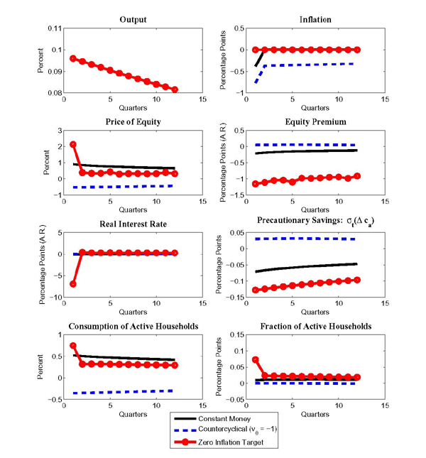
Note: With the exception of the zero inflation target, the monetary policy rule is given by:
where ![]() is the
economy's money growth rate,
is the
economy's money growth rate, ![]() is aggregate
output, and
is aggregate
output, and ![]() denotes the average money growth
rate. Under the zero inflation target,
denotes the average money growth
rate. Under the zero inflation target, ![]() is
chosen so that inflation is constant and equal to
zero.
is
chosen so that inflation is constant and equal to
zero.
Data for Figure 4
| Quarters | Output: Red | Output: Black | Inflation: Blue | Inflation: Red | Price of Equity: Black | Price of Equity: Blue | Price of Equity: Red | Equity Premium: Black | Equity Premium: Blue | Equity Premium: Red | Real Interest Rate: Black | Real Interest Rate: Blue | Real Interest Rate: Red | Precautionary Savings: Black | Precautionary Savings: Blue | Precautionary Savings: Red | Consumption of Active Households: Black | Consumption of Active Households: Blue | Consumption of Active Households: Red | Fraction of Active Households: Black | Fraction of Active Households: Blue | Fraction of Active Households: Red |
|---|---|---|---|---|---|---|---|---|---|---|---|---|---|---|---|---|---|---|---|---|---|---|
| 1 | 0.096 | -0.384 | -0.768 | -0.3456 | 0.90845 | -0.51493 | 0.5742 | -0.21012 | 0.049994 | -0.28706 | -0.08321 | 0.014683 | 0.21832 | -0.07118 | 0.030588 | -0.10609 | 0.52151 | -0.35193 | 0.45736 | 0.010152 | -5.53E-05 | 0.025446 |
| 2 | 0.094589 | 0.005645 | -0.37271 | 0.04348 | 0.85701 | -0.50899 | 0.57636 | -0.18731 | 0.051667 | -0.25332 | -0.03706 | 0.017872 | 0.16902 | -0.06689 | 0.031087 | -0.09527 | 0.50464 | -0.34742 | 0.45402 | 0.010982 | -0.00019 | 0.024094 |
| 3 | 0.093198 | 0.005562 | -0.36723 | 0.042841 | 0.81989 | -0.50189 | 0.573 | -0.1721 | 0.052935 | -0.23101 | -0.01542 | 0.01951 | 0.14431 | -0.06355 | 0.031514 | -0.08792 | 0.49142 | -0.34261 | 0.4493 | 0.011445 | -0.00036 | 0.023199 |
| 4 | 0.091828 | 0.00548 | -0.36183 | 0.042211 | 0.79049 | -0.4941 | 0.56796 | -0.1607 | 0.05371 | -0.21455 | -0.00325 | 0.02008 | 0.12879 | -0.06074 | 0.031782 | -0.08233 | 0.48019 | -0.33765 | 0.44419 | 0.01172 | -0.00053 | 0.022504 |
| 5 | 0.090478 | 0.0054 | -0.35651 | 0.041591 | 0.76596 | -0.48597 | 0.56233 | -0.15168 | 0.054061 | -0.20172 | 0.004158 | 0.020145 | 0.11772 | -0.05833 | 0.031895 | -0.07784 | 0.47023 | -0.33264 | 0.43896 | 0.011879 | -0.00069 | 0.021919 |
| 6 | 0.089148 | 0.00532 | -0.35127 | 0.04098 | 0.74474 | -0.47772 | 0.55649 | -0.14424 | 0.054055 | -0.1913 | 0.008853 | 0.020017 | 0.10913 | -0.05619 | 0.031871 | -0.0741 | 0.46116 | -0.32761 | 0.4337 | 0.011962 | -0.00083 | 0.021401 |
| 7 | 0.087838 | 0.005242 | -0.34611 | 0.040377 | 0.72594 | -0.46944 | 0.55058 | -0.13793 | 0.053773 | -0.18258 | 0.011866 | 0.01983 | 0.10208 | -0.05428 | 0.031736 | -0.0709 | 0.45274 | -0.32261 | 0.42845 | 0.011992 | -0.00095 | 0.020929 |
| 8 | 0.086547 | 0.005165 | -0.34102 | 0.039784 | 0.70894 | -0.4612 | 0.54464 | -0.13246 | 0.053277 | -0.17509 | 0.013822 | 0.019617 | 0.096113 | -0.05254 | 0.03151 | -0.0681 | 0.44483 | -0.31765 | 0.42323 | 0.011981 | -0.00105 | 0.020489 |
| 9 | 0.085274 | 0.005089 | -0.33601 | 0.039199 | 0.69335 | -0.45305 | 0.53869 | -0.1276 | 0.052609 | -0.16848 | 0.015041 | 0.019422 | 0.090885 | -0.05095 | 0.031216 | -0.0656 | 0.4373 | -0.31274 | 0.41803 | 0.011941 | -0.00113 | 0.020072 |
| 10 | 0.084021 | 0.005014 | -0.33107 | 0.038623 | 0.67888 | -0.44502 | 0.53274 | -0.12319 | 0.051814 | -0.16253 | 0.015681 | 0.019285 | 0.086147 | -0.04948 | 0.030867 | -0.06336 | 0.43011 | -0.30789 | 0.41286 | 0.011877 | -0.00119 | 0.019675 |
| 11 | 0.082786 | 0.00494 | -0.3262 | 0.038055 | 0.66533 | -0.43711 | 0.52679 | -0.11917 | 0.05095 | -0.15715 | 0.015911 | 0.019183 | 0.081818 | -0.04811 | 0.03047 | -0.06131 | 0.42318 | -0.30311 | 0.40772 | 0.011794 | -0.00123 | 0.019292 |
| 12 | 0.081569 | 0.004868 | -0.32141 | 0.037495 | 0.65254 | -0.42934 | 0.52084 | -0.11551 | 0.050041 | -0.15225 | 0.015894 | 0.019085 | 0.077874 | -0.04681 | 0.030037 | -0.05941 | 0.41647 | -0.29838 | 0.40261 | 0.011696 | -0.00126 | 0.018923 |
Figure 5. Welfare Distribution for Alternative Monetary Policy Rules
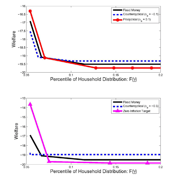
Note: With the exception of the zero inflation target, the monetary policy rule is given by:
where ![]() is the
economy's money growth rate,
is the
economy's money growth rate, ![]() is aggregate
output, and
is aggregate
output, and ![]() denotes the average money growth
rate. Under the zero inflation target,
denotes the average money growth
rate. Under the zero inflation target, ![]() is
chosen so that inflation is constant and equal to
zero.
is
chosen so that inflation is constant and equal to
zero.
Data for Figure 5
| Percentile of household distribution | Top Panel: Black | Top Panel: Blue | Top Panel: Red | Bottom Panel: Black | Bottom Panel: Blue | Bottom Panel: Pink |
|---|---|---|---|---|---|---|
| 0.0543 | -16.906 | -17.527 | -16.303 | -16.906 | -18.775 | -13.659 |
| 0.066906 | -19.082 | -19.086 | -19.12 | -19.082 | -18.965 | -19.709 |
| 0.11467 | -19.507 | -19.318 | -19.734 | -19.507 | -18.955 | -19.845 |
| 0.13401 | -19.507 | -19.318 | -19.734 | -19.507 | -18.955 | -19.845 |
| 0.15438 | -19.507 | -19.318 | -19.734 | -19.507 | -18.955 | -19.845 |
| 0.17537 | -19.507 | -19.318 | -19.734 | -19.507 | -18.955 | -19.845 |
| 0.19668 | -19.507 | -19.318 | -19.734 | -19.507 | -18.955 | -19.845 |
| 0.21806 | -19.507 | -19.318 | -19.734 | -19.507 | -18.955 | -19.845 |
Footnotes
1. We thank Fernando Alvarez, Martin Bodenstein, V.V. Chari, Mike Dotsey, Marc Giannoni, Luca Guerrieri, Ricardo Nunes, and Ken West for useful comments. The views expressed in this paper are solely the responsibility of the authors and should not be interpreted as reflecting the views of the Board of Governors of the Federal Reserve System or of any other person associated with the Federal Reserve System.. Return to text
2. Corresponding Author: Christopher Gust. Emails: [email protected], [email protected]. Return to text
3. For prominent examples of this research agenda, see the collection of papers in (Taylor 1999). Return to text
4. See Bernanke and Kuttner (2005). Additional evidence reinforcing the influence of monetary policy shocks on equity prices include Ehrmann and Fratzscher (2004), Ammer, Vega, and Wongswan (2008), and references therein. Return to text
5. Our model is related to the analysis of Alvarez, Atkeson, and Kehoe (2002) and Khan and Thomas (2007). They introduce endogenously segmented markets into an otherwise standard cash-in-advance economy. An important difference in our model is that we allow households to set up an initial non-state contingent plan that transfers a predetermined amount of funds across their brokerage and checking accounts at future dates. As discussed later, this feature is crucial in delivering quantitatively reasonable asset pricing implications. Return to text
6. See, for example, Calvet, Campbell, and Sodini (2009), Bilias, Georgarakos, and Haliassos (2008) and Brunnermeier and Nagel (2008). Return to text
7. Our approach is similar to Gabaix and Laibson (2001) and Bacchetta and van Wincoop (2009); however, we emphasize that the decision to reoptimize portfolio holdings is state dependent rather than time dependent. Our approach also shares similarities with Reis (2006), who derives inattentive behavior on the part of households who infrequently adjust their consumption and saving plans. Return to text
8. We follow Alvarez, Atkeson, and Kehoe (2002) and model this cost as a physical cost instead of one that reduces an agent's utility. Return to text
9. See, for example, Souleles (2003) and Ameriks and Zeldes (2004). Return to text
10. A
household can reoptimize by setting
![]() , thereby transferring
additional cash from her checking to brokerage account. Similarly,
a household is free to choose
, thereby transferring
additional cash from her checking to brokerage account. Similarly,
a household is free to choose
![]() . Return to text
. Return to text
11. We have abstracted from the possibility that a household may want to save extra cash in their checking and/or brokerage accounts since equations (6) and (7) always bind. Since incorporating occasionally binding constraints greatly complicates the analysis, we address it in Gust and López-Salido (2009a). As discussed there, the asset pricing implications of our analysis are robust to this possibility. Return to text
12. To derive equation (13), one needs to combine equations (7) and (12) with the money market clearing condition:
![$\displaystyle M_t = \int^{\infty}_{0} \left\{ M(s^{t-1},\gamma )+P(s^t)\left[x(s^{t},\gamma ) + \textrm{exp}(\eta t) \gamma \right] z(s^{t},\gamma ) + P(s^t)\textrm{exp}(\eta t)A(s_0,\gamma) \right\} f(\gamma) d\gamma. $](img86.gif)
13. For
convenience we have switched notation to express both the expected
return on equity and the covariance between the pricing kernel and
the return on equity, which are both conditional on the state of
the world at date ![]() . Return to text
. Return to text
14. See, for example, Brunnermeier and Nagel (2008) and Bonaparte and Cooper (2009). Return to text
15. We use
the calibrated parameters discussed above except that there is a
single household that always rebalances (i.e., ![]() ). Return to
text
). Return to
text
16. To
understand why the sensitivity of active consumption increases for
larger values of ![]() , consider a simple example in
which there is one type of household with
, consider a simple example in
which there is one type of household with ![]() and another with
and another with
![]() who receives
who receives
![]() . From the
resource constraint, it follows that
. From the
resource constraint, it follows that
![]() . In the
absence of the non-state contingent plan (i.e.,
. In the
absence of the non-state contingent plan (i.e., ![]() ), unanticipated increase in technology shocks lead to
relatively large increases in
), unanticipated increase in technology shocks lead to
relatively large increases in ![]() and hence
relatively smaller increases in
and hence
relatively smaller increases in ![]() . As the value of
. As the value of ![]() increases, the sensitivity of
increases, the sensitivity of ![]() to technology shocks rises. Return to text
to technology shocks rises. Return to text
17. Following
Hamilton (1994), we define the impulse response of variable, ![]() , at date
, at date ![]() to a
monetary innovation that occurs at date 1 as:
to a
monetary innovation that occurs at date 1 as:
![]() , where
, where ![]() denotes the conditional expectations
operator. Return to text
denotes the conditional expectations
operator. Return to text
18. We provide a graphical representation of this intuition in an earlier version of this paper, Gust and López-Salido (2009b). Return to text
19. This
effect is partially offset by a small increase in the number of
active households resulting from the higher value of ![]() . Return to
text
. Return to
text
20. Holding
the fraction of rebalancers fixed, an offsetting effect is that
increasing
![]() raises the unconditional
volatility of money growth, increasing the volatility of active
consumption growth and hence the average equity
premium. Return to text
raises the unconditional
volatility of money growth, increasing the volatility of active
consumption growth and hence the average equity
premium. Return to text
21. We
determine the function ![]() using equation
(16) under the
constant money growth rule and use this distribution to compute
welfare under the alternative policy rules shown in Table 2. We use the
values of the shocks associated with the nonstochastic steady state
for
using equation
(16) under the
constant money growth rule and use this distribution to compute
welfare under the alternative policy rules shown in Table 2. We use the
values of the shocks associated with the nonstochastic steady state
for ![]() . For further details, see the
appendix. Return to text
. For further details, see the
appendix. Return to text
This version is optimized for use by screen readers. Descriptions for all mathematical expressions are provided in LaTex format. A printable pdf version is available. Return to text