The Federal Reserve Board eagle logo links to home page

Skip to: [Printable Version (PDF)] [Bibliography] [Footnotes]
International Research Forum on Monetary Policy: Screen Reader version

The Heterogeneous Expectations Hypothesis:
Some Evidence from the Lab *

Cars Hommes
CeNDEF, School of Economics, University of Amsterdam,
Roetersstraat 11, NL-1018 WB Amsterdam, Netherlands

Keywords: Heterogeneous Expectations, bounded rationality, learning, heuristics switching.

Abstract:

This paper surveys learning to forecast experiments (LtFEs) with human subjects to test theories of expectations and learning. Subjects must repeatedly forecast a market price, whose realization is an aggregation of individual forecasts. Emphasis is given to how individual forecasting rules interact at the micro level and which structure they co-create at the aggregate, macro level. In particular, we focus on the question wether the evidence from laboratory experiments is consistent with heterogeneous expectations.

"Recent theoretical work is making it increasingly clear that the multiplicity of equilibria ... can arise in a wide variety of situations involving sequential trading, in competitive as well as finite-agent games. All but a few of these equilibria are, I believe, behaviorally uninteresting: They do not describe behavior that collections of adaptively behaving people would ever hit on. I think an appropriate stability theory can be useful in weeding out these uninteresting equilibria ... But to be useful, stability theory must be more than simply a fancy way of saying that one does not want to think about certain equilibria. I prefer to view it as an experimentally testable hypothesis, as a special instance of the adaptive laws that we believe govern all human behavior" (Lucas, 1986, pp. S424-425).


1 Introduction

Individual expectations about future aggregate outcomes is the key feature that distinguishes social sciences and economics from the natural sciences. Daily weather forecasts, either by the public or by experts, do not affect the probability of rain. In contrast, overly optimistic expectations about the economic outlook may have exaggerated the strong rise in world wide financial markets in the late 1990s and, more recently, the excessive growth in housing prices in 2000-2008, while an overly pessimistic outlook by the public and by economists may have amplified the recent financial crisis and deepened the current economic crisis.

Economic decisions today thus depend upon expectations about the future state of the economy. A theory of individual expectations or market beliefs is therefore a crucial part of economic theory. The market is an expectations feedback system and any dynamic economic model depends crucially upon its underlying expectations hypothesis. But how then should one model individuals who learn from the past and adapt their behavior as more and more market realizations become available over time?

Since the seminal works of Muth (1961) and Lucas (1972), the Rational Expectations Hypothesis (REH) has become the leading paradigm on expectation formation in economics, and rational expectations representative agent models have become the mainstream tool of analysis. In such a framework, all agents are the same and forecast rationally, using all available information. Rational expectations are by assumption model consistent and coincide on average with realizations, without systematic forecasting errors. The rational expectations (RE) approach has important advantages: it is simple, elegant and puts strong discipline on individual (forecasting) behavior minimizing the number of free parameters. But drawbacks of the rational agent paradigm are also well known: it is unrealistic in assuming perfect knowledge about the economy (typically it assumes knowledge of the law of motion of the economy) and, even if such knowledge were known, RE requires extremely strong computing abilities of the agents to compute the equilibrium. Most importantly, RE models are at odds with empirical observations and behavior in laboratory experiments wit human subjects and, for example, the decline of worldwide financial markets by almost 50% between October 2008 and March 2009 is hard to reconcile with rational behavior.

Economics, or at least a significant part of it, is currently witnessing a paradigm shift to an alternative, behavioral view, where agents are boundedly rational. This alternative view dates back to Simon (1957) and contains many elements from psychology, e.g. through the work of Tversky and Kahnemann (1974). The need for a new paradigm in economics has recently been forcefully advocated by Akerlof and Shiller (2009), Colander et al. (2009) and DeGrauwe (2009). Concerning expectations of boundedly rational agents, an alternative theory of adaptive learning has been developed, see e.g. Sargent (1993) for an early and Evans and Honkapohja (2001) for a more detailed overview. Boundedly rational agents do not know the law of motion of the economy, but instead use time series observations to form expectations and adapt their behavior trying to learn model parameters of their perceived law of motion as more observations become available. Adaptive learning sometimes enforces convergence to REE, but it may also lead to non-RE equilibria, such as the learning equilibria in Bullard (1994). Adaptive learning models are sometimes "cautious modifications of rational expectations theories" (Sargent, 2008, p26) and other times large deviations from rationality explaining excess volatility through expectations driven fluctuations (Grandmont, 1998). Bounded rationality however also has important drawbacks. In particular, the `wilderness" of bounded rationality (Sims, 1980) leads to (too) many degrees of freedom and too many free parameters. There are simply too many ways of modeling non-rational behavior. This "wilderness" of bounded rationality, seems particularly relevant when individuals have heterogeneous expectations.

A rough estimate indicates that in the past 20 years more than 1000 papers on bounded rationality and learning have appeared. Among these, in the last decade hundreds of (theoretical) papers on agent-based models populated with boundedly rational agents employing heterogeneous strategies/expectations have appeared, especially with applications in finance; see the comprehensive surveys of LeBaron (2006) and Hommes (2006) in the Handbook of Computational Economics Volume 2: Agent-Based Computational Economics (Tesfatsion and Judd, 2006 and very recent surveys by Hommes and Wagener (2009) and Chiarella et al. (2009) in the Handbook of Financial Markets: Dynamics and Evolution (Hens and Schenk-Hoppé, 2009) as well as papers and references in the Handbook of Economic Complexity (Rosser, 2009)1. Most of these papers present stylized, theoretical models or larger, agent-based simulation models, with the realistic feature that these models can mimic many stylized facts in financial time series (Lux, 2009) and in macro data (Delli-Gatti et al., 2008).

The empirical validation of heterogeneity is an important area of current research. For example, Baak (1999) and Chavas (2000) estimate heterogeneous agent models (HAMs) on hog and beef market data, and found empirical evidence for heterogeneity of expectations. For the beef market Chavas (2000) estimates that about 47% of the beef producers behave naively (using only the last price in their forecast), 18% of the beef producers behaves rationally, whereas 35% behaves quasi-rationally (i.e. use a univariate autoregressive time series model to forecast prices). A number of recent contributions have estimated heterogeneous agent models with fundamentalists and chartist strategies on stock prices (e.g. Boswijk et al. (2007), de Jong, Verschoor and Zwinkels (2009), exchange rates (e.g. Gilli and Winker (2003), Westerhoff and Reitz (2003) and several commodities (e.g. gold prices (Alfarano et al., 2005), and oil prices (ter Ellen and Zwinkels, 2009)). Most of these studies find significant time-variation in the fractions of agents using a mean-reverting fundamental versus a trend-following strategy. Empirical evidence for heterogeneous trading strategies in the Spanish Stock Market Exchange has been found in Vaglica et al. (2008); in particular, Lillo et al. (2008) show that the investors can be classified in different groups, including trend followers and contrarians, whose change of inventory of the stock is positively respectively negatively correlated with stock return.

A related, complementary branch of empirical literature uses survey data to measure individual expectations; see Pesaran and Weale (2006) for a stimulating overview. An advantage of survey data analysis is that it can focus exclusively on the expectations-generating process, avoiding the dilemma of testing joint hypotheses. There is quite some evidence on forecasting heterogeneity in survey data. For example, Frankel and Froot (1987, 1990), Allen and Taylor (1990) and Taylor and Allen (1992) already found that financial experts use different forecasting strategies to predict exchange rates. They tend to use trend extrapolating rules at short horizons (up to 3 months) and mean-reverting fundamentalists rules at longer horizons (6 months to 1 year) and, moreover, the weight given to different forecasting techniques changes over time. Vissing-Jorgensen (2003) presents evidence of heterogeneous beliefs of individual investors about the prospect of the stock market, while Shiller (2000) finds evidence that investor's sentiment changes over time, with both institutions and individual investors becoming more optimistic in response to recent significant increases of the stock market. Evidence concerning heterogeneity in survey data on exchange rate expectations can also be found in MacDonald and Marsh (1996), Elliott and Ito (1999), Prat and Uctum (2000) and Bénassy-Quéré et al. (2003). Dreger and Stadtmann (2008) show that for exchange rate forecasts at a 6 months horizon, different expectations about macroeconomic fundamentals is what drives heterogeneity. Mankiw et al. (2003) find evidence for heterogeneity in inflation expectations in the Michigan Survey of Consumers and show that the data are inconsistent with either rational or adaptive expectations, but may be consistent with a sticky information model. Capistrán and Timmermann (2009) show that heterogeneity of inflation expectations of professional forecasters varies systematically over time, and depends on the level and the variance of current inflation. Pfajfar and Santoro (2009) measure the degree of heterogeneity in private agents' inflation forecasts by exploring time series of percentiles from the empirical distribution of survey data. They show that heterogeneity in inflation expectations is pervasive and identify three regions of the distribution corresponding to different expectations formation mechanisms: a static or highly autoregressive region on the left hand side of the median, a nearly rational region around the median and a fraction of forecasts on the right hand side of the median consistent with adaptive learning and sticky information. Branch (2004, 2007) estimates a simple switching model with heterogeneous expectations, along the lines of Brock and Hommes (1997), and provides empirical evidence suggesting that models which allow the degree of heterogeneity to change over time provide a better fit on exchange rate survey data.

In this paper, we discuss laboratory experiments with human subjects that can be used to validate expectations hypotheses and learning models. Lucas (1986) already stressed the importance of laboratory experiments in studying adaptive learning and its stability (see the quote at the beginning). In particular, we are interested in the potential role of heterogeneity in expectations. We quote from Muth (1961, p.321, emphasis added) on expectations heterogeneity and its aggregate effect: "Allowing for cross-sectional differences in expectations is a simple matter, because their aggregate affect is negligible as long as the deviation from the rational forecast for an individual firm is not strongly correlated with those of the others. Modifications are necessary only if the correlation of the errors is large and depends systematically on other explanatory variables"

In this paper we discuss learning to forecast experiments (LtFEs) which provide a controlled laboratory environment to study individual expectations as well as aggregate outcomes, and investigate questions such as:

The goals of this paper are twofold. Firstly, we summarize a number of LtFEs in different market environments. Secondly, we fit a theory of heterogeneous expectations to the experimental data and discuss how well the model explains the data across different market settings. This poses a particular challenge: is there a general, perhaps even a universal theory of heterogeneous expectations, that is, can one come up with one single expectations hypothesis explaining all LtFEs across different market settings?

The paper is organized as follows. Section 2 summarizes related literature on experiments on expectations. Section 3 discusses an experiment in a cobweb market modeling framework, while Section 4 describes an asset pricing experiment. Section 5 presents a simple forecasting heuristics switching model, where agents switch between different forecasting rules based upon their recent performance, and fits the model to the asset pricing experiments. In Section 6 the same switching model is fitted to experimental data in different market settings, where the only difference comes from the type of expectations feedback, positive versus negative. Section 7 briefly discusses some recent experiments in a New Keynesian macro setting and Section 8 concludes.


2 Learning-to-forecast experiments (LtFEs)

Laboratory experiments with human subjects, with full control over the market environment and economic fundamentals, form an ideal tool to study interactions at the micro-level and how individual behavior affects aggregate market outcomes. Duffy (2008ab) provides stimulating and up to date surveys of "experimental macroeconomics". Early work in this area focussed on market mechanisms, such as double auctions, and the availability of information and futures markets, ensuring that equilibrium will be reached (e.g. Smith (1962), Plott ad Sunder (1982), Sunder (1995) and Plott and Smith (20xx)). More recently, unstable market environments where equilibrium may not be reached, but instead bubbles and crashes may arise have also been designed (e.g. Smith et al. (1988) and Lei et al. (2001).

In experimental work expectations often plays an indirect or implicit role. However, in order to avoid joint hypothesis testing there is an expanding literature on exclusive experimental testing of the expectations hypothesis. An early example is Schmalensee (1976), who presents subjects with historical data on wheat prices and asks them to predict the mean wheat price for the next 5 periods. Williams (1987) considers expectation formation in an experimental double auction market, which varies from period to period by small shifts in the market clearing price. Participants predict the mean contract price for 4 or 5 consecutive periods and the participant with the lowest forecast error earns $1.00. In Dwyer et al. (1993) and Hey (1994) subjects have to predict a time series generated by an (exogenous) stochastic process such as a random walk or a simple linear first order autoregressive process. Kelley and Friedman (2002) consider learning in an Orange Juice Futures price forecasting experiment, where prices are driven by a linear stochastic process with two exogenous variables (weather and competing supply). But in these papers there is no expectations feedback, since market realizations are not affected by individual forecasts.

Here, we focus on so-called learning-to-forecast experiments (LtFEs), where subject's only task is to forecast the price of some commodity for a number, say 50-60, periods, with the realized market price in each period determined by (average) individual expectations. In LtFEs subjects' forecasting decisions are thus separated from market-trading decisions. The subjects in the experiments do not participate themselves directly in other market activities, such as trading or producing, but are forecasters (e.g. advisors to large producers or financial investors) whose earnings increase when forecasting errors decrease. At the beginning of each period, individual forecasts are collected, which feed directly into (unknown) demand and/or supply functions and computerized trading yields a market price, derived from equilibrium between aggregate demand and supply, that becomes available to the subjects at the end of the period. Demand and supply curves are derived from maximization of expected utility, profit or wealth and thus consistent with rational optimizing behavior.

These LtFEs were motivated by the bounded rationality literature, in order to distinguish between different theories of expectations and learning. Sargent (1993), for example, emphasizes two different requirements of rational expectations. The first requirement imposes that individuals maximize an objective function (utility, profit, wealth, etc.) subject to perceived constraints, while the second requirement imposes mutual consistency of these perceptions. Marimon and Sunder (1994) were the first to set up experiments testing individual rationality and mutual consistency either jointly or separately and used different experimental designs to distinguish between "learning-to-optimize" versus "learning-to-forecast" experiments (Marimon and Sunder, 1994, p.134). The LtFEs focus exclusively on the role of expectations, using computerized optimal individual demand and supply schedules once these individual forecasts have been made.

In LtFEs, subjects typically only have qualitative information about the market. They know that the price  p_t is an aggregation of individual forecasts, derived from equilibrium between demand and supply and are able to infer the type of expectations feedback, positive or negative. Positive (negative) feedback means that an increase of (average) individual forecasts leads to a higher (lower) market equilibrium price. Positive feedback is important in speculative asset markets, where higher market expectations lead to an increase of speculative demand and therefore an increase of the realized asset price. Negative feedback may be dominant in supply driven commodity markets, where an increase in expected prices leads to higher production and thus to a lower realized market price. Subjects in the LtFEs know past prices and their own past forecasts and earnings, typically in table as well as in graphic form, as illustrated by an example in Figure 1. They do however not know the forecasts of other participants, the exact market equilibrium equation, the exact demand and supply schedules and the exact number of other demanders and/or suppliers in the market. The type of information in the experiment is thus very similar to models of bounded rationality and adaptive learning, were agents try to learn a perceived law of motion, based upon time series observations without knowing the underlying actual law of motion of the market.

Figure 1: Typical computerscreen in Learning to Forecast Experiment

Figure 1: Typical computer screen in Learning to Forecast Experiment
Figure 1 is a screen shot that contains several different boxes. In the upper left there is a line graph showing the number versus the round, with two lines: one for the prediction and one for the real number.  On the right side there is a table giving the values of the points for both lines.  Right underneath the graph there is a box with three subsections, which lists the total earnings, the earnings in this period, and the remaining time.  Below that box is another box with two subsections, which contains the question "What is your prediction this period? Your prediction must be between 0 and 100" and then in the second box there is a space to enter your prediction.

Quite a number of LtFEs have appeared in the literature. In a series of papers, Marimon, Spear and Sunder studied expectation formation in inflationary overlapping generations economies. Marimon, Spear and Sunder (1993) find experimental evidence for expectationally driven cycles and coordination of beliefs on a sunspot 2-cycle equilibrium, but only after agents have been exposed to exogenous shocks of a similar kind. Marimon and Sunder (1995) present experimental evidence that a "simple" rule, such as a constant growth of the money supply, can help coordinate agents' beliefs and help stabilize the economy. More recently, a number of LtFEs within other macro economic frameworks have been performed. Adam (2007) uses a simple model of sticky prices and shows that a restricted perception equilibrium explains the experimental data better than the RE benchmark solution. Pfajfar and Santoro (2009) and Assenza et al. (2009) run LtFEs in a new Keynesian framework. Pfajfar and Santoro (2009) find evidence for heterogeneity of expectations in their experimental data and three different types of forecasting rules: simple heuristics (e.g. trend following rules), adaptive learning and rational expectations. The LtFEs of Assenza et al. (2009) will be briefly discussed in Section 7.

A learning to forecast experiment may be seen as a test bed for the expectations hypothesis in a benchmark model, assuming that all other assumptions such as rational, utility and profit maximizing behavior are satisfied. A learning to forecast experiment thus provides clean data on individual expectations as well as aggregate price behavior. Here we will discuss learning to forecast experiments, based on three benchmark models: (1) the cobweb model, (2) a standard asset pricing model and (3) a New Keynesian macro model. The underlying laws of motion are of the form

\displaystyle p_t \displaystyle = \displaystyle F(p^e_{1,t}, \cdots, p^e_{H,t}) \hskip4.7cm   cobweb (2.1)
\displaystyle %f(\bar{p}_{t}^e) p_t \displaystyle = \displaystyle F(p^e_{1,t+1}, \cdots, p^e_{H,t+1}) \hskip3.9cm   asset pricing (2.2)
\displaystyle % f(\bar{p}_{t+1}^e) (\pi_t,y_t) \displaystyle = \displaystyle F(\pi^e_{1,t+1}, \cdots, \pi^e_{H,t+1}; y^e_{1,t+1}, \cdots, y^e_{H,t+1}). \hskip0.5cm   New Keynesian\displaystyle %f(\bar{\pi}_{t+1}^e,\bar{y}_{t+1}^e) (2.3)

In the cobweb LtFE experiments in Hommes al. (2007), the realized market price  p_t in (2.1) is a (nonlinear) function of all individual one-period ahead forecasts  p_{h,t}^e. In the asset pricing LtFE in Hommes et al. (2005a, 2008) the realized market price  p_t in (2.2) is a (nonlinear) function of all two-period ahead individual forecasts  p_{h,t+1}^e of next periods price  p_{t+1}. There is another important difference between the cobweb and the asset pricing LtFEs: negative versus positive expectations feedback. Positive feedback means that the realized market price increases, when an individual price forecast increases. This feature is characteristic of speculative asset markets, where an increase of the price forecast leads to higher demand for the asset and therefore to higher market prices; mathematically it means that the map  F in (2.2) is an increasing function of individual forecasts. Negative feedback prevails in supply driven markets, where a higher expected price leads to increased production and thus a lower realized market price; the map  F in (2.1) underlying the cobweb experiments is decreasing in individual forecasts. In Section 6 we review the LtFE of Heemeijer et al. (2009), comparing positive versus negative feedback systems. Despite the fact that the only difference is the sign (positive versus negative) of the coefficient in the linear price-expectations feedback rule, the aggregate price behaviors and individual expectations turn out to be rather different.

Finally, in the New Keynesian macro model expectations on two different variables interact and realized inflation  \pi_t and realized output gap  y_t in (2.3) simultaneously depend (linearly) on all two-period ahead individual forecasts of both inflation and the output gap. In Section 7 we will briefly discuss the LtFE of Assenza et al. (2009), where the dynamics of inflation and the output gap is driven simultaneously by individual expectations of both inflation and the output gap.


3 Cobweb Experiments

In this section we discuss LtFE in the classical cobweb framework. This is exactly the same framework employed in the seminal paper of Muth (1961) introducing rational expectations. These cobweb LtFEs may thus be seen as a direct test of the REH in the cobweb model, assuming all other modeling assumptions (e.g. producers' profit maximization and consumers utility maximization) are satisfied. Carlson (1967) already conducted hand-run experiments with subjects as cobweb suppliers. Holt and Villamil (1986) and Hommes et al. (2000) conducted individual cobweb experiments, where price fluctuations are induced by decisions of a single individual. Wellford (1989) conducted several computerized cobweb experiments, where market prices were determined by subjects’ quantity decisions.

Here we focus on the LtFEs in Hommes et al. (2007) with  K=6 participants per session. The participants were asked to predict next period's price of a commodity under limited information on the structural characteristics of the market. Participants were only informed about the basic principles of the cobweb-type market. They were advisors to producers, whose only job is to accurately forecast the price of the good for 50 subsequent periods. Pay-offs were defined as a quadratic function of squared forecasting errors, truncated at 0:2

\displaystyle E=Max\displaystyle \{1300-260(p_{i,t}^e-p_t^*)^2,\ 0\}. (3.1)

Participants were informed that the price would be determined by market clearing and that it would have to be within the range  [0,10]. Furthermore, they knew that there was (negative) feedback from individual price forecasts to realized market price in the sense that if their forecast would increase, the supply would increase and consequently the market clearing price would decrease. Subjects however did not know how large these feedback effects would be, as they had no knowledge of underlying market equilibrium equations. Subjects thus had qualitative information about the market, but no quantitative details.

The realized price  p_t in the experiments was determined by the (unknown) market equilibrium between demand and supply:

\displaystyle D(p_t) = \sum_{i=1}^K S(p_{i,t}^e), (3.2)

with  p_{i,t}^e the price forecast of participant  i at time  t. Demand was exogenously given by a simple linear schedule:
\displaystyle D(p_t)=a-dp_t+\eta_t (3.3)

with  \eta_{t} a small stochastic shock drawn from a Normal distribution representing small random demand fluctuations. Supply  S(p_{i,t}^e) was determined by the nonlinear schedule
\displaystyle S(p_{i,t}^e)=tanh\displaystyle (\lambda(p_{i,t}^e-6))+1. (3.4)

This increasing, nonlinear supply schedule can be derived from producer's expected profit maximization with a convex cost function. Subjects in the experiment thus do not participate themselves in production decisions, but supply is computed as if each individual producer maximizes expected profit, given his/her individual price forecast. The parameter  \lambda tunes the nonlinearity of the supply curve and the stability of the underlying cobweb model. The resulting equilibrium price is obtained as:
\displaystyle p_t = D^{-1}(\sum_{i=1}^K S(p_{i,t}^e)) = \frac{a-\sum_{i=1}^K S(p_{i,t}^e)}{d} + \epsilon_t, (3.5)

where  \epsilon_t=\eta_t/d. Given the parameters  a,d and  \lambda the aggregate realized price  p_t depends on individual price expectations as well as the realization of the (small) stochastic shocks. While the parameters of the demand function and the realizations of the noise component remained unchanged across all treatments at  a=13.8,  d=1.5 and  \epsilon_{t}=\frac{\eta_{t}}{d}\sim N(0,0.5), the slope parameter of the supply function was varied. Here we consider two treatments. A stable treatment had  \lambda=0.22, for which under naive expectations the price converges quickly to the rational expectations equilibrium. In another strongly unstable treatment, with  \lambda=2, under naive expectations the RE price is unstable and prices converge to a 2-cycle, as illustrated in Fig. 2. Along the 2-cycle producers are "irrational" in the sense that they make systematic forecasting errors, predicting a high (low) price when realized market price will be low (high).

Figure 2: Cobweb dynamics in the strongly unstable treatment in two benchmark simulations. Left Panel: convergence to a (noisy) 2-cycle under naive expectations. Right Panel: convergence to (noisy) RE equilibrium price under learning by average.
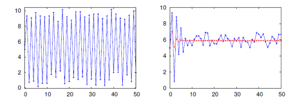
Figure 2: Cobweb dynamics in the strongly unstable treatment in two benchmark simulations. Left Panel: convergence to a (noisy) 2-cycle under naive expectations. Right Panel: convergence to a (noise) RE equilibrium price under learning by average.
Figure 2 has two panels, each containing a line graph with y-axes from 0 to 10 and x-axes from 0 to 50.  In the left  graph, a blue line starts at 5 and then first shoots up before rapidly oscillating in between close to zero and close to ten for the duration of the graph, reaching almost zero 24 times and almost 10 25 times.  The right graph has a blue line and a red line. The blue line starts at 5 and then shoots up to almost ten like in the left graph, but this time is quickly dampened and by the x-value of 10 the blue line oscillates around a value of six with peaks and troughs of about 1. The red line also starts at 5 and also initially increases, though by much less than the blue line. It oscillates a few times before ending on the value of 6 and staying there for the duration of the graph.

Figure 3: Cobweb Learning to Forecast Experiments Top Panels: stable: coordination on RE unstable: persistent heterogeneity Middle Panels: Bottom Panels: degree of heterogeneity measured by standard deviations of individual forecasts (6 individuals) averaged over the six groups in each treatment.
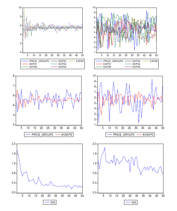
Figure 3: Cobweb Learning to Forecast Experiments Top Panels: stable: coordination on RE unstable: persistent heterogeneity Middle Panels: Bottom Panels: degree of heterogeneity measured by standard deviation of individual forecasts (6 individuals) arranged over the six groups in each treatment
Figure 3 contains 6 line graphs which all have x-axes that go from 0 to 50, and y-axes that vary. The first two line graphs contain have y-axes that go from 0 to 10 and have seven lines - the blue line is Price_Group2, the red line is Exp21, the green line is Exp22, the black line is Exp23, the teal line is exp24, the purple line is exp25, an the olive green line is exp26.  In the first graph, the lines start out fairly volatile, oscillating around the y-value of 5 or so (except for the olive green line which reaches both extremes of the y-axis), but once they reach around 10 they don't fluctuate as much and their mean value shifts up to about 5.5. All lines continue to fluctuate between about 4.5 and 6.5 for the duration for the graph, except for the dark green line which stays flat at 5 until around 10, when it jumps up to 5.5 and stays there for the rest of the graph.

The second graph also contains all seven lines again, but this time they fluctuate more severely for the entire duration of the graph, oscillating between around 2 and 9. The blue, red and teal and olive green lines fluctuate by the greatest amount.

The third graph has a y-axis that goes from 3 to 8. There is a blue line that represents Price_Group2 and a red line that represents Avexp2.   The blue line starts at 5.5 and initially drops down to almost 4, then fluctuates up and down over a mean value of about 5.5 for the duration of the graph.  The red line starts at 5.75 and initially goes up, and then oscillates back a forth around the value of 5.5 a few times, but by about 15 it fluctuates just a little around the y-value of 5.5.

The fourth graph has a y-axis that goes from 0 to 2. There is a blue line that represents price_group3 and a red line that represents Avexp3.  The blue line starts at 8 and then oscillates rapidly between the boundaries of 8 and 1.5. For the last third of the graph, the blue line only reaches as low as 4 but reaches as high as 9.5. The red line starts at 5.5 and also oscillates rapidly, though not as much as the blue line. It stays between roughly 7 and 5 for the whole graph, and by the end stays between around 6 and 5.

The fifth graph has a y-axis that goes from 0 to 2, and contains just a blue line that represents sig.  The line starts at around 1.7 and then rapidly falls to .7 by around 5, where it increases just slightly before dropping down again.  The line starts to flatten out and gently fluctuates around .3 for the last half of the graph.

The sixth graph has y-axis that goes from 0 to 2, and contains a blue line that represents Sig as well.  The blue line starts at 1.3 and drops down briefly to 1 before increasing again to reach a peak at 1.8.  The line then fluctuates with troughs and peaks about 0.4 apart, all the while with its mean value steadily declining. At the end of the graph, the blue line is fairly stable with a mean of about 0.9 and then fluctuates from 0.8 to 1.1.

Under rational expectations, all individuals would predict the unique price  p^*, at which demand and supply intersect. Given that all individuals have rational expectations, realized prices will be given by

\displaystyle p_t= p^* + \epsilon_t, (3.6)

that is, small random fluctuations around the RE steady state. Given the limited market information one can not expect that all individuals have rational expectations at the outset, but one can hope that in such a simple, stationary environment individuals would learn to have rational expectations. For example, if price expectations are given by the sample average of past prices, convergence to the RE-price is enforced, as illustrated in Fig. 2 (right panel). The LtFE has in fact been designed to test whether individuals are able to learn from their systematic mistakes under naive expectations and coordinate on a learning algorithm enforcing convergence to the RE steady state.

Figure 3 shows time series of realized market prices together with the individual forecasts (top panels) as well as the average forecast (middle panels) for two typical experimental groups, one stable treatment (left panels) and one strongly unstable treatment (right panels). An immediate observation is that in the stable treatment, after a short learning phase of about 10 periods, the price volatility is low and individual forecasts as well as average forecasts are very close to the RE benchmark, with price fluctuations entirely driven by the small random shocks in the experiments. Aggregate price behaviour and individual forecasts are very different in the strongly unstable treatment. Realized prices exhibit large fluctuations, while individual forecasts are very volatile, even towards the end of the experiment. The bottom panel of figure 3 shows the degree of heterogeneity, as measured by the standard deviations of individual forecasts (6 individuals) averaged over the six groups, in the stable respectively the strongly unstable treatments. In the stable treatment heterogeneity quickly decreases over time, showing that individuals coordinate on a forecast close to the RE-benchmark steady state. In the strongly unstable treatment heterogeneity decreases somewhat over time, but only slowly, and remains at least 3 times as high as in the stable treatment. Hence, in the classical cobweb framework used in Muth (1961) to introduce rational expectations, our LtFEs show that only in the stable cobweb case, the interaction of individual forecasting rules enforces convergence to the RE-benchmark. In the unstable treatment, heterogeneity in forecasting is persistent and leads to an aggregate effect upon prices characterized by excess volatility.

The behaviour in Figure 3 is typical for all cobweb experiments. Hommes et al. (2007) summarize the stylized facts of the cobweb LtFE experiments as follows: (1) the sample mean of realized prices is close to the RE benchmark  p^* in all treatments; (2) the sample variance of realized prices depends on the treatment: it is close to the RE benchmark in the stable treatment, but significantly higher in the unstable treatment; (3) realized market prices are irregular and do not exhibit significant linear autocorrelations.

These stylized facts across different treatments appear hard to explain by standard learning mechanisms offered by the theoretical literature. For example, naive expectations are inconsistent with the experiments, because in the unstable treatment it predicts too much regularity (convergence to a 2-cycle) in aggregate price behavior. Average price expectations, which is just the simplest form of adaptive learning obtained when regressing prices on a constant, also are inconsistent with the experiments, because for both treatment it predicts convergence to the RE-benchmark (see Fig. 2, right panel). Hommes (2009) discusses a number of other homogeneous learning algorithms and concludes that heterogeneity in forecasting rules is needed to explain the stylized facts of the cobweb experiments across different treatments. Apparently, the interaction of agents' individual forecasting rules washes out linear predictability in aggregate price behavior. In the stable treatment, this interaction leads to coordination on the "correct" RE benchmark steady state, but in the unstable treatment heterogeneity persists and prices are excessively volatile.

Figure 4: Simulated prices and learning parameters.

Figure 4: Simulated prices and learning parameters
Figure 4 contains four graphs, with the top two graphs representing prices and the bottom two graphs representing forecast parameters.

Both the top two graphs have y-axes that go from 0 to 10 and x-axes that go from 0 to 300. In the first graph, there is a horizontal blue line at the y-value of 5.8 that runs the whole length of the graph.  There is also a black line that rapidly oscillates between about 5 and 6.5, with the blue line appearing as its mean. In the second graph, there is also a horizontal blue line is at the y-value of about 6, and there is also a black line that rapidly crosses the blue line and has troughs and peaks of about 4 and 7. The second graph has a black line with a greater range of movement than the first graph.

The bottom two graphs, which represent forecast parameters, have y-axes that go from -2 to 8 and x-axes that go from 0 to 300.  Both graphs contain two lines - a blue line and a green line.  In the first graph, the green line hovers around the y-value of 5.5 or so (which is marked by a dashed black line).  The line is not smooth but rather oscillates quickly but without high amplitude, with occasional spikes.  The blue line hovers around the y-value of 0 (which is also marked by a dashed black line) and also has small oscillations with small amplitude, though it has less spikes than the green line, and in general the amplitude of its spikes is less than that of the green line.  The second of the bottom graphs is very similar to the first, though this time the green line hovers around the y-value of 6 and it has more frequent spikes of larger amplitude. The blue line still hovers around 0, but has increased amplitude of its spikes.

Hommes and Lux (2009) present a model of heterogenous individual learning via genetic algorithms (GAs) to explain the cobweb LtFEs3. Genetic algorithms require a functional specification of the forecasting rule, whose fitness-maximizing parameter values are searched for via the evolutionary algorithm. Hommes and Lux (2009) use a simple first order autoregressive rule:

\displaystyle p^e_{i, t+1}=\alpha_i+\beta_i(p_t-\alpha_i).     (3.7)

Such a first order autoregressive (AR1) rule seems a natural forecasting scheme as agents could implement it using the sample average as their estimate of  \alpha_i and the first order sample autocorrelation as the estimate of  \beta_i4. Moreover, the AR1 forecasting rule (3.7) has a simple behavioral interpretation, with  \alpha_i representing an anchor or observed average price level around which the market price fluctuates, and  \beta_i representing the observed persistence or anti-persistence of price fluctuations5.

Hommes and Lux (2009) show that the interaction of individual GA-learning rules simultaneously reproduces all stylized facts in aggregate price behaviour observed in the experiments across the different treatments. Figure [*] shows typical price time series under GA-learning as well as time series of the two parameters in the AR1 forecasting rule for the stable treatment (left panel) and the strongly unstable treatment (right panel). In the stable treatment the parameters converge to a neighborhood of the RE benchmark, consistent with the observed coordination of individual forecasts in the experiments, while in the strongly unstable treatment parameters continue to fluctuate and prices keep moving away from the RE-benchmark, consistent with the persistent heterogeneity in the strongly unstable treatment of the experiments (cf. Fig. 3).

4 Asset Pricing Experiment

Before discussing the asset pricing Learning-to-forecast experiments (LtFEs) in Hommes et al. (2005), we briefly discuss the underlying benchmark model.


4.1 An asset pricing model with heterogeneous beliefs

This section discusses a standard one-period asset pricing model, extended to the case with heterogeneous beliefs, as in Campbell et al. (1997) and Brock and Hommes (1998). Agents can either invest in a risk free or in a risky asset. The risk free asset is in perfect elastic supply and pays a fixed rate of return  r; the risky asset pays an uncertain dividend. Let  p_t be the price per share (ex-dividend) of the risky asset at time  t, and let  y_t be the stochastic dividend process of the risky asset. Next period's wealth is given by

\displaystyle W_{t+1} = RW_t + (p_{t+1} + y_{t+1} - Rp_t)z_t, (4.1)

where  R=1+r is the gross rate of risk free return and  z_t denotes the number of shares of the risky asset purchased at date  t. Let  E_{ht} and  V_{ht} denote the `beliefs' or forecasts of trader type  h about conditional expectation and conditional variance. Agents are assumed to be myopic mean-variance maximizers so that the demand  z_{ht} of type  h for the risky asset solves
\displaystyle \hbox{Max}_{z_t}\{E_{ht}[W_{t+1}] - \frac{a}{2} V_{ht}[W_{t+1}]\}, (4.2)

where  a is the risk aversion parameter. The demand  z_{ht} for risky assets by trader type  h is then
\displaystyle z_{ht} = \frac{E_{ht}[p_{t+1}+y_{t+1}-Rp_t]}{aV_{ht}[p_{t+1}+y_{t+1}-Rp_t]}= \frac{E_{ht}[p_{t+1}+y_{t+1}-Rp_t]}{a\sigma^2}, (4.3)

where the conditional variance  V_{ht}=\sigma^2 is assumed to be equal for all types and constant.6 Let  z^s denote the supply of outside risky shares per investor, assumed to be constant, and let  n_{ht} denote the fraction of type  h at date  t. Equilibrium of demand and supply yields
\displaystyle \sum_{h=1}^{H} n_{ht} \frac{E_{ht}[p_{t+1}+y_{t+1}-Rp_t]}{a\sigma^2} = z^s, (4.4)

where  H is the number of different trader types. The forecasts  E_{ht}[p_{t+1}+y_{t+1}] of tomorrows prices and dividends are made before the equilibrium price  p_t has been revealed by the market and therefore will depend upon a publically available information set  I_{t-1} = \{p_{t-1}, p_{t-2}, \ldots; y_{t-1}, y_{t-2}, \ldots\} of past prices and dividends. Solving the heterogeneous market clearing equation for the equilibrium price gives
\displaystyle p_t = \frac{1}{1+r} \sum_{h=1}^{H} n_{ht}E_{ht}[p_{t+1} + y_{t+1}] - a\sigma^2 z^s. (4.5)

The quantity  a\sigma^2 z^s may be interpreted as a risk premium for traders to hold all risky assets. I te experimets discussed below,  z^s=0 so tat (4.5) correspods to te case of risk-eutral ivestors. Moreover, it will be assumed divideds are IID, wit mea  \bar{y}, ad all traders ave correct expectatios about divideds,  E_{ht}[y_{t+1}] = E_{t}[y_{t+1}] = \bar{y}, so tat (4.5) simplifies to
\displaystyle p_t = \frac{1}{1+r} \sum_{h=1}^{H} n_{ht}E_{ht}[p_{t+1}] + \bar{y}. (4.6)

4.2 Experimental Design

In the asset pricing LtFEs six subjects are forecast advisors to large pension funds. Subjects only task is to forecast the price of a risk asset for 50 periods and, based on this forecast, the pension fund ten decides how much to invest in the risky asset according to the mean-variance demand function (4.3). The realized asset price in the experiment is given as

\displaystyle p_t = \frac{1}{1+r} \Big( (1-n_t)\bar{p^e_{t+1}} + n_t\,p^f + \bar{y} + \varepsilon_t \Big)    

where  p^f=\bar{y}/r is the fundamental price,  \bar{p^e_{t+1}} is the average two-period ahead price forecast over six individuals and  \varepsilon_t are small shocks, e.g. representing small random fluctuations in asset demand7. Since the mean-dividend  \bar{y} and the interest rate  r are known to the subjects, they can in principle use these to compute the fundamental price and use it in their forecast. The fraction  n_t in (4.7) is the share of computerized fundamental robot traders, given by
\displaystyle n_t = 1 - \exp \big(- \tfrac{1}{200}\vert p_{t-1} - p^f\vert\big). (4.7)

The fraction of robot traders increases as the price moves further away from the fundamental benchmark. The fundamental trader thus acts as a "far from equilibrium" stabilizing force in the market, mimicking the feature that more traders in the market expect the price to return in the direction of the fundamental when the deviations becomes large8. Subjects' earnings depend on forecasting performance and are given by a quadratic scoring rule
\displaystyle e_{i,t} = \left\{ \begin{array}{cl} 1 - \left(\frac{p_t - p_{i,t}^e}{7}\right)^2 & \text{if} \quad \vert p_t - p_{i,t}^e \vert < 7\,,\\ [0.1cm] 0 & \text{otherwise}\,, \end{array} \right. (4.8)

so that forecasting errors exceeding 7 would result in no reward at a given period. At the end of the session the accumulated earnings of every participant were converted to euros ( 1 point computed as in (4.8) corresponded to 50 cents).


4.3 Benchmark Simulations

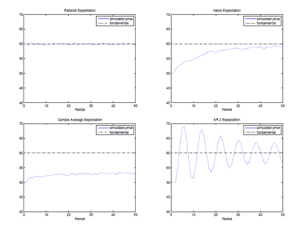
Figure 5: Simulation benchmarks: Top Panels RE (left) and naive (right); Bottom Panels: average expectations (left) ad AR2 trend following rule  p^e_{t+1}= (60+p_{t-1})/2 + (p_{t-1}-p_{t-2}).

Figure 5 contains four line graphs, each containing a horizontal dashed black line set at a y-value of 60, which is labeled "fundamental" and a blue line that is labeled "simulated price".  The x-axes are labeled "Period" and go from 0 to 50, while the y-axes are prices under various expectations and go from 40 to 70.

In the first graph, which is called "Rational Expectation", the blue line fluctuates around the black line very tightly, with an amplitude of about 0.5, for the entire graph.

In the second graph, which is called "Native Expectation", the blue line starts at 50 and slopes upward with decreasing slop, leveling out at about 59 by the end of the graph.

In the third graph, which is called "Sample Average Expectation", the blue line starts at 50 and very gradually increases (with some fluctuation) until it reaches a y-value of 53 at around period 20, then remains there for the rest of the graph.

In the fourth graph, the blue line starts at 50 then very rapidly shoots up to 68 at about period 5, then falls to 52 at period 10, is at 66 for period 15, at 54 for period 20, and so on, decreasing its amplitude by about 2 every cycle of 10 periods.  The last two waves of the blue line have its crests and troughs at 54 and 64.  Overall, the blue line oscillates back and forth across the black line with decreasing amplitude.

Fig. 5 shows the simulation of realized prices, which would occur for a number of homogeneous benchmark expectations rules. When all individuals use the rational, fundamental forecasting rule,  p^{e}_{i,t+1}=\bar{y}/r=p^f, for all  i and  t, the realized price  p_t=\varepsilon_t/(1+r) randomly fluctuates around the fundamental level  p^f=60 with small amplitude, due to the small socks. In the experiment, one can not expect rational behavior at the outset, but aggregate prices might converge to their fundamental value through individual learning. Under naive expectations the price slowly converges towards its fundamental value. The same is true under average expectations, the simplest form of adaptive learning obtained when regressing the price on a constant, but the convergence is extremely slow. If all subjects would use the simple AR2 rule

\displaystyle p^e_{t+1}= \frac{60+p_{t-1}}{2} + (p_{t-1}-p_{t-2}), (4.9)

price oscillations as illustrated in the bottom right panel of Fig. 5 arise. This is an example of an anchoring and adjustment rule, which plays an important role in psychology (Tversky ad Kahneman, 1974), because it extrapolates the last price change from a reference point or anchor  (p^f + p_{t-1})/2 describing the "long-run" price level9.

4.4 Experimental Results

Figure 6: Asset Pricing Experiments: realized market prices, six individual predictions (middle part of each panel) and individual errors (bottom part of each panel).
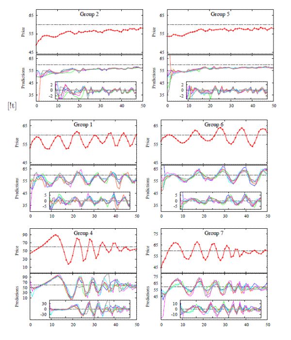
Figure 6: Asset Pricing Experiments: realized market prices, six individual predictions (middle part of each panel) and individual errors (bottom part of each panel).
Figure 6 is contains six panels, each made up of one group that has three line graphs, one on top of the other, with the third within the bottom graph. The top line graph in each group has a y-axis of Price and just a single red line. The bottom line graph has a y-axis of Predictions that goes from under 35 to over 65 and graphs several different lines in different colors. Both line graphs have an x-axis that represents periods and goes from 0 to 50.  The third line graph also contains several lines of different colors.  All three line graphs in each group contain a grey dashed line at the y-value of 60.

The upper left panel displays the graphs for Group 2.  The red line in the top graph (with y-axis limits of 45 and 65) starts at 50 and increases (with a few dips) gradually to around 58. In the bottom graph, most of the lines start between 50 and 55, though the orange line intercepts the y-axis far below the confines of the graph, and meets up with the other lines at about 2 periods in. From there, all the lines move more or less together, slowly sloping upward and ending at a value of about 58.  In the internal third graph (with y-axis limits of -3 and 3), the lines oscillate more or less around zero, with decreasing amplitude.

The upper right panel displays the graphs for Group 5. The red line in the top graph (with y-axis limits of 45 and 65) starts at 54 and slowly increases for the first half of the graph, before reaching and oscillating around 57 or 58 for the remainder of the graph.  In the bottom graph, most of the lines start at 50, except that the orange line intercepts the y-axis far above the upper limit of the y-axis, though it falls shortly to meet up with the other lines at around 50. The Green and black lines also start at 40 and 35 respectively, but rise to around 50 as well.  By the x-value of about 5, all lines more or less move together, slowly increasing until reaching at plateau at around 57. In the internal third graph (with y-axis limits of -3 and 3), the lines oscillate more or less around zero, with decreasing amplitude.

The middle left panel displays the graphs for Group 1. The red line in the top graph (with y-axis limits of 45 and 65) starts at 54 and oscillates fairly regularly with an amplitude of 5 and a wavelength of 9. Throughout the course of the graph the mean value shifts up to only around 55. In the bottom graph, most of the lines start at 50 and oscillate fairly regularly with an amplitude of 5 and a wavelength of 9. The magenta line starts slightly lower at about 30 but quickly rejoins the other lines at 50.  In the internal third graph (with y-axis limits of -5 and 5), the lines oscillate fairly regularly around 0 with a consistent of amplitude of about 4.

The middle right panel displays the graphs for Group 6.  The red line in the top graph (with y-axis limits of 45 and 65) starts at 56 and oscillates around 58 with an initial amplitude of 4 and wavelength of 11. The median increases to about 58 by the end of the graph. In the bottom graph, most of the lines start at 45 and then swing upwards where they oscillate around 59 or so with a wavelength of about 10, for the remainder of the graph.   Both the magenta and the blue lines start at a higher value and then drop down to meet up with the rest of the lines.  In the internal third graph (with y-axis limits of -5 and 5), the lines first rise just barely over 0, but then they oscillate around 0 with increasing amplitude.  The blue and magenta lines first start from a high y-value then drop down to join the other lines.

The bottom left panel displays the graphs for Group 4.  The red line in the top graph (with y-axis limits of 10 and 90) starts at about 45 and gradually rises to 90 before quickly dropping down at an x-value of 12 and oscillating around 50 with decreasing amplitude.  In the bottom graph, all the lines mimic the shape of the red line - first there is a long increase to about ninety, then rapid oscillations with decreasing amplitude.  Towards the end of the bottom graph, the lines do no stay together as they do in the beginning.  In the internal third graph (with y-axis limits of -30 and 30), the lines stay at around zero before beginning to oscillate fairly regularly at an x-value of almost 30 and with amplitude of about 30.  Like the bottom graph, the lines are fairly uniform in the beginning but do not stay together by the end.

The bottom right panel displays the graphs for Group 7.  The red line in the top graph starts at 45 and increases to over 65, before oscillating with decreasing amplitude and a wavelength of about 12 until the end of the graph.   In the bottom graph, all the lines start at around 50 and oscillate around 0 with decreasing amplitude and decreasing wavelength.    In the internal third graph (with y-axis limits of -10 and 10) the lines start at about 10 and swoop down, with a slightly elongated first wavelength, but then they oscillate about 0 with an amplitude of about 10, before dampening to 0 at the end.

Fig. 6 shows time series of prices, individual predictions and forecasting errors in six different markets of the experiment. A striking feature of aggregate price behavior is that three different qualitative patterns emerge. The prices in groups  2 and 5 converge slowly and almost monotonically to the fundamental price level. In groups 1 and 6 persistent oscillations are observed during the entire experiment. In groups 4 and 7 prices are also fluctuating but their amplitude is decreasing.10

A second striking result concerns individual predictions. In all groups participants were able to coordinate their forecasting activity. The forecasts, as shown in the lower parts of the panels in Fig. 7, are dispersed in the first periods but then become very close to each other in all groups. The coordination of individual forecasts has been achieved in the absence of any communication between subjects and knowledge of past and present predictions of other participants.

Figure 7: Left Panels: prices for laboratory experiments in three different groups. Lower parts of left panels show individual predictions and forecasting errors (inner frames). Right Panels: Evolution of the degree of heterogeneity as measured by the standard deviation of individual forecasts in corresponding groups.
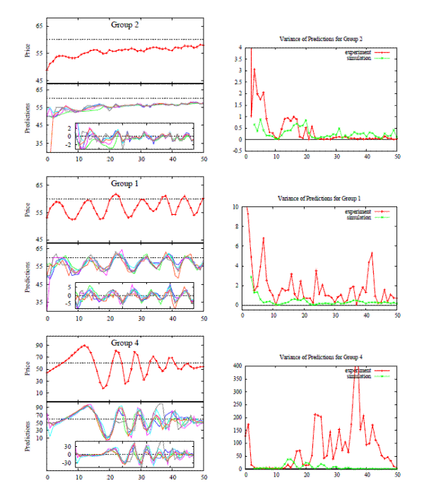
Figure 7: Left Panels: prices for laboratory experiments in three different groups. Lower parts of left panels show individual predictions and forecasting errors (inner frames). Right Panels: Evolution of the degree of heterogeneity as measured by the standard deviation of individual forecasts in corresponding groups
Figure 7 contains three sets of two graphs (together by group number.) The sets contain two graphs (on the left and on the right.) The graphs on the left are split into three separate line graphs like in Figure 6, with the top part graphing a red line representing price over time, and the bottom two graphs showing lines of several different colors representing predictions and forecasting errors over time (respectively.)  The right graph depicts the Variance of Predictions for the group, with two lines; the red line represents the experiment, and the green line represents the simulation. 

The top panel of Figure 7 is for Group 2. The price line on the top left graph starts at around 48 and gradually increases to about 58 by the end of the graph (with a few dips along the way.) The bottom graph of predictions has most of the lines start in between 50 and 55, with the exception of the orange line that starts from much lower (perhaps around 20 though its y-intercept is out of the range of the graph) but rises steeply to meet up with the rest of the line within 5 periods.  From there, the lines generally stay together and very gradually rise to about 57 by the end of the graph.  The forecasting error graph shows most of the line starting at around 2, and then oscillating with decreased amplitude about 0.  The Variance of Predictions graph for Group 2 has the red line intercepting the y-axis well out of the range of the graph (which runs from y=-0.5 to y = 4) and drops down sharply to 1 in the first two periods, then it shoots up again to 3, then to 2, 1.75, 2, and then it drops sharply almost zero 10 periods in.  It then goes back up to around 1 for 8 periods but then mainly stays around zero for the rest of the graph.  The green line starts at 0.75, goes to 9 by 10 periods in, then back up to about 1 20 periods in, and then bounces along zero for the remainder of the graph.

The middle panel of Figure 7 is for Group 1. The price line on the top left graph starts at 53 and goes upward to 59, and then oscillates between 60 and 53 with a slight upward trend and with a period of about 9 for the remainder of the graph.  The bottom graph of predictions mimics the shape almost exactly.  The graph of forecasting errors has most lines starting at around 1, and then oscillating around 0 with decreasing amplitude (amplitude of 1 by the end) and periods of about 9.  The Variance of Predictions graph for Group 1 has the red line intercepting above the confines of the graph (which runs from 0 to 10 on the y-axis) and then quickly dropping down to less than 2 in the first few periods. It then bounces back to 7, then down to 0, where it then goes between 0 and 4 with varying amplitude. It goes to six at around period 40, but then drops down again near 0 for the remainder of the graph. The green line starts at 3 and drops quickly down to 0 by the first 10 periods, and it stays near zero for the remainder of the graph.

The bottom panel of Figure 7 is for Group 4.   The price line on the top left graph starts at 45 and then slowly sweeps upward, topping out at 90 at period 12 before sharply falling to 10, and then oscillating about 50 with decreased amplitude and period of about 9 for the remainder of the graph.  The bottom graph of predictions mimics the shape of the top graph almost exactly, with the liens very uniform in the beginning of the graph though disjointed by the end.  The bottom graph of forecasting errors has most line staring at around 0 and staying there until about 18, when the lines bump up to about thirty, and then oscillate about 0 with slightly decreased amplitude. Like the graph of predictions, the lines are uniformly together in the part of the graph but then disjointed by the end.  The Variance of Predictions graph for Group 4 has the red line starting at 125 and increasing slightly to 175 in the first few periods, then dropping done and staying near 0 until the 13th period, where it has sporadic jumps of about 100, trending upward. But in the last ten periods of the graph, the red line decreases to end at around 0 by the end of the graph.  The green line starts at 0 and stays there until increasing with a slight bump at period 11 to a height of 50, and then oscillates with decreasing amplitude before plateauing at 0 at about 35 and remaining there for the rest of the graph.

Figure 7 (right panel) illustrates the degree of heterogeneity, as measured by the standard deviation of individual forecasts, in three different groups. A first observation is that for each of the three groups, there is considerable time variation in the degree of heterogeneity. In the converging group 2 heterogeneity quickly decreases, to a level below 1 after period 15 and close to 0 after period 25. It should be noted that despite the fact that coordination is quick, prices are not close to the fundamental value. Hence, coordination on the "wrong", non-fundamental price occurs. In the oscillating group 1, heterogeneity fluctuates, with stronger coordination (i.e. a smaller degree of heterogeneity) during trends and weaker coordination during trend reversals. The same features, but in a more extreme form, arise in the dampened oscillation group 4. During the strong trend from periods 4-13 coordination is very strong, with the degree of heterogeneity falling from a initial level above 150 to values less than 5. Thereafter, coordination weakens and the degree of heterogeneity peaks at price trend reversals, becomes very high after period 23 (note the scale on the vertical axis) with an extremely high peak around period 36-37. Note that, as heterogeneity increases, the asset price stabilizes.

To summarize, in the asset pricing LtFEs we observe the following stylized facts:

  1. participants were unable to learn the rational, fundamental price; only in some cases individual predictions moved (slowly) in the direction of the fundamental price towards the end of the experiment;
  2. alltough the sessions were designed in exactly the same, three different price patterns were observed: (i) slow, (almost) monotonic convergence, (ii) persistent price oscillations with almost constant amplitude, and (iii) large initial oscillations dampening slowly towards the end of the experiment;
  3. already after a short transient, participants were able to coordinate their forecasting activity, submitting similar forecasts in every period.

One would like to have a model explaining all these stylized facts simultaneously. We have not bee able to come up wit a homogeneous expectations model fitting all these experiments. The fact that qualitatively different aggregate outcomes can arise suggests that path dependence and heterogeneous expectations play a key role.


5 A Heterogeneous Expectations Model

In the last 15 years a large literature on heterogenous agent models has developed, as surveyed e.g. by Hommes (2006) ad LeBaron(2006). In particular, Brock ad Hommes (1997) introduced a heterogeneous expectations model, where agents tend to switch towards forecasting strategies that have performed better in the recent past. Here we discuss a modified version, a heuristics switching model, which has recently been fitted to the asset pricing LtFEs by Anufriev and Hommes (2009)11.

Agents can choose from a number of simple forecasting heuristics. To discipline the wilderness of bounded rationality, the set of forecasting heuristics needs to be carefully chosen. We will choose forecasting heuristics that are similar to those obtained from estimations of linear models on individual forecasting data in the LtFEs in Hommes et al. (2005) and Heemeijer et al. (2009). To further discipline the wilderness of bounded rationality two forms of individual learning are introduced. First, for some heuristics adaptive learning takes place, tat is, some parameters of the heuristics are updated over time. Second, evolutionar selection or performance based reinforcement learning takes place, that is, agents evaluate the performances of all heuristics, and tend to switch to more successfully rules. Hence, the impact of each of the rules is evolving over time.

To keep the model as simple as possible, Anufriev and Hommes (2009) restricted attention to only four forecasting heuristics:

ADA\displaystyle \quad p^e_{1,t+1} \displaystyle = \displaystyle 0.65\,p_{t-1} + 0.35\,p^e_{1,t} (5.1)
WTR\displaystyle \quad p^e_{2,t+1} \displaystyle = \displaystyle p_{t-1}+ 0.4\,(p_{t-1}-p_{t-2}) (5.2)
STR\displaystyle \quad p^e_{3,t+1} \displaystyle = \displaystyle p_{t-1}+ 1.3\,(p_{t-1}-p_{t-2}) (5.3)
LAA\displaystyle \quad p^e_{4,t+1} \displaystyle = \displaystyle \frac{p^{av}_{t-1}+ p_{t-1}}{2} + (p_{t-1}-p_{t-2}), (5.4)

were  p^{av}_{t-1}=\sum_{j=0}^{t-1}p_j is the sample average of past prices. The first adaptive expectations (ADA) rule predicts that the price is a weighted average of the last observed price  p_{t-1} and the last price forecast  p^e_{t}. This ADA rule was obtained as the estimated linear rule of a number of subjects in the converging groups 2 and 5. The second and the third rules are both trend following rules, with a weak trend (WTR) parameter 0.4 and a strong trend (STR) parameter  1.3 respectively12. These rules were obtained as the estimated linear rules for quite a number of subjects in the oscillatory markets 1, 4, 6 and 7, with 0.4 ad 1.3 obtained as the smallest and largest trend extrapolating coefficients. Finally, the fourth rule is an anchor and adjustment rule, obtained from the linear AR2 rule (4.9), discussed in subsection 4.3, by replacing the (unknown) fundamental price  p^f by a proxy given by the (observable) sample average of past prices  p^{av}_{t-1}. The weight coefficient of the ADA rule and the trend parameters of trend following rules have been fixed and it appears that the simulations below are robust with respect small changes of these parameters. The LAA rule exhibits a simple form of adaptive learning, since the anchor of the rule is the average of the last observed price and the sample average of all observed prices.

Subjects switch between the different forecasting rules based upon quadratic forecasting errors, consistent with the earnings incentives in the experiments. The fitness or performance measure of forecasting heuristic  i is given by

\displaystyle U_{i,t-1} = -\big(p_{t-1}-p^e_{i,t-1}\big)^2+\eta\,U_{i,t-2}\, (5.5)

where the parameter  \eta \in [0,1] measure the strength of the agents' memory. Switching is described by a discrete choice model with asynchronous updating
\displaystyle n_{i,t} = \delta\,n_{i,t-1}+(1-\delta)\,\frac{\exp(\beta\,U_{i,t-1})}{\sum_{i=1}^4 \exp(\beta\,U_{i,t-1})} (5.6)

In the special case  \delta=0, (5.6) reduces to the the discrete choice model with synchronous updating used in Brock and Hommes (1997). The more general case,  0 \leq \delta \leq 1, gives some persistence or inertia in the impact of rule  h, reflecting the fact (consistent with the experimental data) that not all the participants update their rule in every period or at the same time (see Hommes et al., 2005b and Diks and van der Weide, 2005). Hence,  \delta may be interpreted as the average per period fraction of individuals who stick to their previous strategy. In the extreme case  \delta=1, the initial impacts of the rules never change; if  0 < \delta \leq 1, in each period a fraction  1-\delta of participants update their rule according to the discrete choice model. The parameter  \beta \geq 0 represents the intensity of choice measuring how sensitive individuals are to differences in strategy performance. The higher the intensity of choice  \beta, the faster individuals will switch to more successful rules. In the extreme case  \beta=0, the impacts in (5.6) move to an equal distribution independent of their past performance. At the other extreme  \beta=\infty, all agents who update their heuristic (i.e., a fraction  1-\delta) switch to the most successful predictor.

In all simulations below, we fix the parameters at the benchmark values  \beta=0.4, \eta=0.7, \delta= 0.913 and the initial fractions of the four strategies are equal, i.e.  n_{ht}=0.25. The simulations thus only differ in their initial prices, which have been chosen exactly the same as in the first two periods in the corresponding experimental group

Figure 8: Left Panels: prices for laboratory experiments in different groups (red) with corresponding one-step ahead predictions of the evolutionary model (blue). Lower parts of left panels show predictions and forecasting errors (inner frames) of four heuristics. Right Panels: Evolution of heuristic impacts during the one-step ahead predictions of the model. Fractions of four forecasting heuristics: adaptive expectations (ADA, purple), weak trend followers (WTR, black), strong trend followers (STR, blue) and anchoring adjustment heuristic (LAA, red).
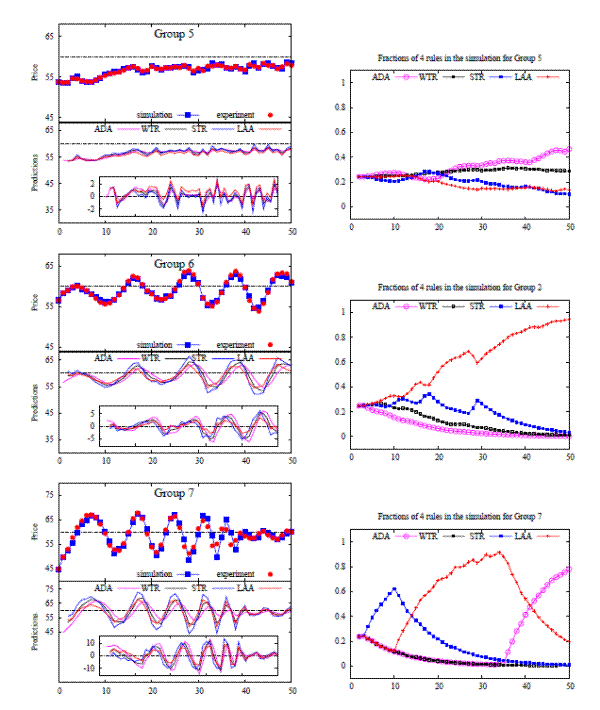
Figure 8: Left panels - prices for laboratory experiments in different groups (red) with corresponding one-step ahead predictions of the evolution model (blue).  Lower parts of left panels show predictions and forecasting errors (inner frames) of four heuristics. Right panels - evolution of heuristic impacts during the one-step ahead predictions of the model. Fractions of four forecasting heuristics: adaptive expectation (ADA, purple), weak trend followers (WTR, black), strong trend followers (STR, blue) and anchoring adjustment heuristic (LAA, red).

Figure 8 contains three sets of line graphs; one set each for Group 5, Group 6 and Group 7.  In the left graphs, there is a top graph which represents Price (with y-limits of 45 and 65) and has a blue line for the simulation and a red line for the experiment, as well as a dashed black line where price equals 60.  The bottom left graph (with limits of 35 to 65) has a pink line for ADA, a grey line for WTR, a blue line for STR and a red line for LAA, as well as a dashed black line at the y-value of 60.  Both graphs have an x-axis that goes from 0 to 50. Within the bottom graph, there are the forecasting errors with the same respective colors and varying limits.  On the right, there is a graph representing the Fractions of 4 rules in the simulation of each group, and there is a pink line for ADA, a black line for WTR, and blue line for STR and a red line for LAA.  The y-limits are 0 to 1 and the x-limits are from 0 to 50.

The first set of graphs is for Group 5.  In the graph for price, the red and blue lines follow an almost identical path which starts at about 54 and, with a few jumps and dips, slowly rises to 58 by the end of the graph.  In the predictions graph, the lines follow the same path as in the price graph.  In the forecasting errors graph (which has y-axis limits of -2 and 2), the lines stay together for the most part, with the pink and red lines above the blue and grey lines for most of the graph.  The lines start out at 0 and rise to 2 before falling sharply and then rising more slowly, all in the first ten periods.  They then sharply rise and fall across the x-axis with a period of about 5 for the remainder of the graph.  The right hand graph has all four lines starting at 0.2, and then they diverge. The pink line rises a fraction, then dips, and then steadily rises to 0.5 by the end of the graph. The blue line dips, then rises, then falls steadily to 0.1 by the end of the graph. The black line gradually increases and then plateaus at 0.3. The red line gradually falls and is at .15 by the end of the graph.

The second set of graphs is for Group 6.  In the graph for price, the red and blue lines follow an almost identical path which starts at about 56 and then rises to about 60, then falls back to 56 at 10 periods, then rises to 63 and back down to 57 in the next then periods, then rises to 65 and then to 55 in its next ten periods and then has a nearly identical phase before ending at around 63 on its way down.  In the predictions graph, the lines follow the nearly the same path as in the price graph, with all four lines staying generally together.  In the forecasting errors graph (which has y-axis limits of -5 and 5), the lines also stay together for the most part.  The lines start out at 0 and fall slightly before rising and falling again with increased amplitude to the end of the graph.  The right hand graph has all four lines starting at 0.2. The pink line falls with decreasing steepness to plateau at 0 by end of the graph. The blue line dips, then rises, then dips for longer, then has one last rise before steadily declining to 0 by the end of the graph. The black line gradually decreases and then plateaus at 0. The red line quickly rises, with only a few dips, and ends the graph at 1.

The third set of graphs is for Group 7.  In the graph for price, the red and blue lines follow an almost identical path which starts at 45 and then rises to about 65, then oscillates around 60 with a decreasing wave length and mildly decreasing amplitude. At about 40 periods the wave is dampened almost entirely and barely wavers around 60 until the end of the graph.  In the predictions graph, the lines follow the nearly the same path as in the price graph, with all four lines staying generally together.  In the forecasting errors graph (which has y-axis limits of -10 and 10), the lines also stay pretty much together and follow a nearly identical path (though scaled down) from the predictions graph.  The right hand graph has all four lines starting at 0.2. The black line just steadily decreases and plateaus at 0 by the end of the graph. The pink stays with the black line until 35 periods in when it rises sharply though with decreasing steepness, until ending at 0.8 at the end of the graph. The blue line rises sharply to 0.6 then falls with decreasing steepness and plateaus at 0 by the end of the graph. The red line stays with the black and pink lines until 10 when it increases sharply, reaching a point of nearly 1 at 35, then falls sharply to end at 0.2 at the end of the graph.

Fig. 8 compares the experimental data with the one-step ahead predictions made by the heuristics switching model, for one converging group (group 5), one oscillating group (group 6) and one dampened oscillating group (group 7); the other groups yield very similar results; see Anufriev and Hommes (2009). Fig. 8 suggests that the switching model with four heuristics fits the experimental data quite nicely. The one-step ahead predictions of the nonlinear switching model in Fig. 8 use past experimental price data to determine the forecasts and the fractions of the strategies at each period  t, i.e., the model simulation uses exactly the same information that was available to participants in the experiments. An immediate observations by comparing these simulations is that the one-period ahead forecasts can easily follow the different patterns in aggregate price behavior, slow monotonic convergence, sustained oscillations as well as dampened oscillations.

The right panels in Fig. 8 show the corresponding fractions of the four strategies for each group. In different groups different heuristics are taking the lead after starting from a uniform distribution. In the monotonically converging group, the impact of the different rules stays more or less equal, although the impact of adaptive expectations gradually increases and slightly dominates the other rules in the last 25 periods. The oscillatory group yields similar results as, with the LAA rule dominating the market early and its impact increasing to about  90\% towards the end of the experiment. Finally, for the group with the dampened oscillations, one step ahead forecast produces a rich evolutionary selection dynamics (bottom panel), with three different phases where the STR, the LAA and the ADA heuristics subsequently dominate. The STR dominates during the initial phase of a strong trend in prices, but starts declining after it misses the first turning point of the trend. The LAA does a better job in predicting the trend reversal and its impact starts increasing. The LAA takes the lead in the second phase of the experiment, with oscillating prices. But the oscillations slowly dampen and therefore, after period 35, the impact of adaptive expectations, which has been the worst performing rule until that point, starts increasing and adaptive expectations dominates the groups in the last 9 periods.


6 Positive versus Negative Feedback Experiments

Aggregate price behavior in the cobweb and the asset pricing LtFEs are quite different. While in the cobweb framework the price fluctuates around its fundamental value, with a sample average of realized prices very close to the RE price, in the asset pricing experiments persistent deviations from the fundamental price with long lasting under- or over-valuations have been observed. A key difference between the cobweb and asset pricing experiments is the type of feedback: the asset pricing (cobweb) framework exhibits positive (negative) feedback, that is the realized price depends positively (negatively) on the average price forecast. In the case of positive (negative) feedback, when an individual forecast increases, the realized market price goes up (down). A natural question then is whether the type of feedback, positive versus negative, explains these differences in aggregate behavior.

In most markets both types of feedback may play a role. Positive feedback however, seems particularly relevant in speculative asset markets. If many agents expect the price of an asset to rise they will start buying the asset, aggregate demand will increase and so, by the law of supply and demand, will the asset price. High price expectations thus become self-confirming and lead to high realized asset prices. In markets where the role of speculative demand is less important, e.g. in markets for non-storable commodities, negative feedback may play a more prominent role. Consider e.g. a supply-driven commodity market. If many producers expect future prices to be high they will increase production which, according to the law of supply and demand, will lead to a low realized market price.

Heemeijer et al. (2009) investigate how the expectations feedback structure affects individual forecasting behaviour and aggregate market outcomes by considering market environments that only differ in the sign of the expectations feedback, but are equivalent along all other dimensions. In this section we discuss these experiments and apply the heterogeneous expectations model of Section 5 to see whether it can explain the different aggregate outcomes.

The distinction between positive and negative expectation feedback is related to the concepts of strategic complements versus strategic substitutes. Haltiwanger and Waldman (1985) argue that when actions are strategic complements, agents have an incentive to imitate other agents. This is the case in an asset market, where predicting a price close to the predictions of the other participants turns out to be most profitable. However, coordination of predictions enhances the impact of the irrational participants upon realized prices and convergence to the rational equilibrium price becomes unlikely. When actions are strategic substitutes, agents have an incentive to deviate from what other agents are doing. This is the case in negative feedback markets, where agents have an incentive to predict high (low) prices when the majority predicts prices below (above) the equilibrium price. The impact of irrational individuals will be limited and convergence to the equilibrium price is more likely. Coordination of predictions will only take place after convergence.

In recent experiments Fehr and Tyran (2001, 2005, 2007) study the impact of different strategic environments (strategic complementarity versus strategic substitutability) on individual rationality and aggregate outcomes. Strategic substitutability (complementarity) prevails if an increase in the action of individual i generates an incentive for j to decrease (increase) his action. Fehr and Tyran study the adjustment of nominal prices after an anticipated money shock in a price setting game with positively (complements) or negatively sloped (substitutes) reaction curves, and find much faster convergence in the case of substitutes. Sutan and Willinger (2009) investigate a new variant of beauty contest games (BCG) in which players actions are strategic substitutes versus strategic complements and find that chosen numbers are closer to rational play in the case of strategic substitutes.

In the LtFEs of Heemeijer et al. (2009), the (unknown) price generating rules in the negative and positive feedback systems were respectively:

\displaystyle p_t = 60 - \frac{20}{21}[\sum_{h=1}^6 \frac{1}{6} p_{ht}^e] - 60] + \epsilon_t, \hskip2cm   negative feedback (6.1)

\displaystyle p_t = 60 + \frac{20}{21}[\sum_{h=1}^6 \frac{1}{6} p_{ht}^e - 60] + \epsilon_t, \hskip2cm   positive feedback (6.2)

where  \epsilon_t is a random shock to the pricing rule. First we will consider positive and negative feedback systems with small IID shocks  \epsilon_t,  \epsilon_t\sim N(0,0.25), and later on with large permanent shocks.

A common feature of the positive and negative feedback systems (6.1) and (6.2) is that both have the same RE equilibrium steady state  p^*, with  p^*=60 when the shocks  \epsilon_t have mean 0. The only difference between (6.1) and (6.2) is therefore the sign of the slope of the linear map,  20/21\approx +0.95 resp.  -20/21\approx -0.9514.

Figure 9: Negative (left panel) vs. positive (right panel) feedback experiments with small IID shocks; prices (top panels), individual predictions (bottom panels) and forecast errors (small panels).
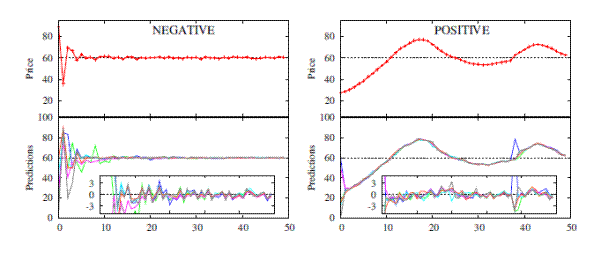
Figure 9: Negative (left panel) vs. positive (right panel) feedback experiments with small IID shocks; prices (top panels), individual predictions (bottom panels) and forecast errors (small panels).
Figure 9 contains two panels which are split into three line graphs. There is the top graph which represents price with a red line, the bottom graph which represents predictions and has several differently colored lines, and the inner graph that represents forecasting errors and has the same color lines as in the bottom graph.

The left panel shows line graphs for the negative feedback case.  In the price graph (which has y-limits of 0 and 90) the red line starts at 90 and falls sharply to 35, then rises again to 70, then falls to 60 where it remains, with very slight disturbances, until the end of the graph.  In the predictions graph, most all the lines follow a nearly identical path of the price line in the top graph.  In the forecast error graphs, the y-limits are -4 and 4, and while most lines start out of the graph, by 10 periods in most of the lines are together and oscillating around 0.

The right panel shows the graphs for the positive feedback case. In the price graph (which has y-limits of 0 and 90), the red line starts at 30 and gradually increases to 8 by 20 periods in, and then falls to 55 about 40 periods in, then rises to 70 and decreases almost to 60 by the end of the graph.  In the predictions graph, most all of the lines follows a nearly identical path, with the exception that all the lines start either at 60 or at 0 but very soon converge on the set path, and also just before 40 periods in blue line spikes up by 20 before settling back into the path again.  In the forecast error graphs, the y-limits are -4 and 4, and most of the lines oscillate around 0 for the remainder of the graph.  The blue line spikes up past the boundaries of the graph right before 40.

Figure 9 shows realized market prices as well as individual predictions in two typical groups. A striking feature is that aggregate price behavior is very different in the positive versus negative feedback cases. In the negative feedback case, the price relatively quickly settles down to the RE steady state price 60, while in the positive feedback case, the market price oscillates slowly around its fundamental value. Individual forecasting behavior is also different for the different feedback treatments: in the case of positive feedback, coordination of individual forecasts occurs extremely quickly, within 2-3 periods. The coordination however is on a "wrong" non-fundamental price. In contrast, in the negative feedback case coordination of individual forecasts is slower and takes about 10 periods. More persistence in heterogeneity of individual forecasts however ensures that, after 10 periods, the realized market price is very close to the RE benchmark of 60.

Figure 10: Positive feedback (bottom panels) and negative feedback (top panels) markets with small shocks. Realized and simulated prices (left panels) and corresponding evolution of fractions of 4 strategies in heuristics switching model.
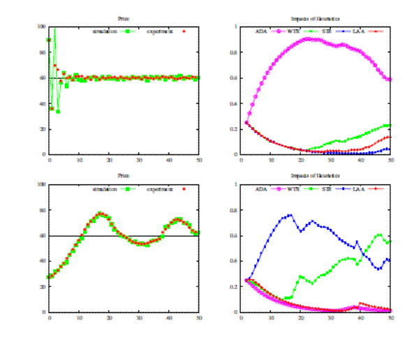
Figure 10: Positive feedback (bottom panels) and negative feedback (top panels) markets with small shocks. Realized and simulated prices (left panels) and corresponding evolution of fractions of 4 strategies in heuristics switching model.
Figure 10 contains four line graphs in a two-by-two formation. The left-side graphs are for the price and they have two lines, a green one for the simulation and a red one for the experiment, and the y-axis goes from 0 to 100 (the x-axis goes from 0 to 50 periods).  The right-side graphs are for the impact of heuristics and there are four lines: there is a pink one for ADA, a green one for WTR, a blue one for STR and a red one for LAA. The y-axis goes from 0 to 1 and the x-axis goes from 0 to 50 periods.

The two top graphs are for negative feedback. The price graph has both the red and green lines starting at 90, and then dropping to 35. Then the green line goes up past 100 but the red line goes to only 70. The red line oscillates very lightly around 60, while the green line takes a few more ups and downs until it also oscillates around 60.  The impacts of heuristics graph has all four lines starting at about 0.25. Then the red line gradually drops down and heads up again when it hits almost zero, creating a gentle u-shape, ending at 0.15 by the end of the graph.  The blue line follows the red line but stays at 0 between 30 and 40 periods, and then just barely rises to 0.05 by the end of the graph. The green line stays with the red and green lines until 20 when it heads up again at a steady pace and ends at 0.25 at the end of the graph. The pink line increases rapidly to 0.9 and then falls again, creating a hump, and ends at 0.6.

The two bottom graphs are for positive feedback. The price graph has both the red and green lines following a nearly identical route, with the lines starts at around 28 and then increasing to almost 80 18 periods in, and then decreasing to 55 at 30 periods, then rising again to 70 at 25 and ending at almost 60.  The impacts of heuristics graph has all four lines starting at about 0.25. Then the pink line gradually drops down to 0 at around 30 periods in, then has a small increase at 35 but then drops down again to end at 0.  The red line follows almost an identical path except its slight increase at the end comes about two periods later and is a little higher.  The green line follows the red and pink lines until 15 when it increases with irregular dips and rises, until ending at 0.55. The blue line increases sharply after its start and tops out at 0.7 before decreasing again, with a few dips and rises in between, until it ends at 0.4.

Can the heterogeneous expectations model of Section 5 explain these different outcomes in individual and aggregate behaviour? Figure 10 shows realized market prices together with the simulated prices (left panels), and the corresponding evolution of the fractions of the four strategies (right panels) of the heuristics switching model with the same benchmark parameters as before, i.e.  \beta=0.4, \eta=0.7, \delta= 0.9. The model matches aggregate price behaviour in both the negative and positive feedback treatment. Furthermore, the time series of the fractions of the different forecasting heuristics (Figure 10, right panels) provide an intuitive explanation of why aggregate behavior is different. In the negative feedback treatment, the adaptive expectations strategy performs best and within 20 periods it captures more than  90\% of the market, thus enforcing convergence towards the fundamental equilibrium price. In contrast, in the positive feedback treatment the impact of the strong trend-following rule (STR) quickly increases and it captures more than  75\% of the market after 15 periods. Thereafter, the impact of the STR rule gradually declines, while the fraction of weak trend-followers (WTR) gradually increases due to the fact that the STR-rule makes (somewhat) larger mistakes (especially at the turning points) than the WTR-rule.

The difference in aggregate behavior is thus explained by the fact that trend following rules are successful in a positive feedback environment reinforcing price oscillations and persistent deviations from the fundamental equilibrium benchmark price, while the trend-following rules are driven out by adaptive expectations in the case of negative feedback.

Figure 11: Positive feedback (bottom panels) and negative feedback (top panels) markets with large permanent shocks to the equilibrium steady state level. Realized and simulated prices (left panels) and corresponding evolution of fractions of the 4 strategies in heuristics switching model.
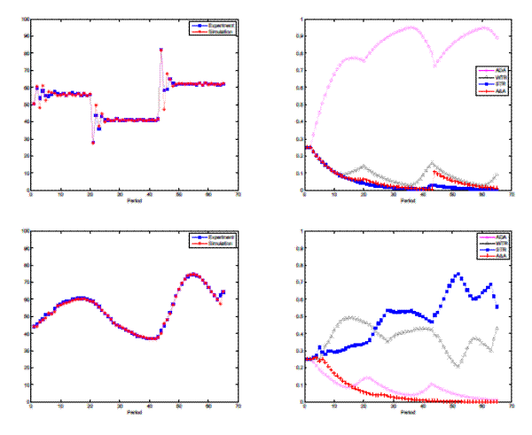
Figure 11: Positive feedback (bottom panels) and negative feedback (top panels) markets with large permanent shocks to the equilibrium steady state level. Realized and simulated prices (left panels) and corresponding evolution of fractions of the 4 strategies in heuristics switching model.
Figure 11 contains four line graphs in a two-by-two formation. The left-side graphs are for the price and they have a red line for the simulation, and a blue line for the experiment.  The y-axis goes from 0 to 100 (the x-axis goes from 0 to 70 periods).  The right-side graphs are for the evolution of fractions and contain four lines: there is a pink one for ADA, a grey one for WTR, a blue one for STR and a red one for A&A. The y-axis goes from 0 to 1 and the x-axis goes from 0 to 70 periods.

The two top graphs are for negative feedback. In the price graph, both lines start at 50 and then bounce back between 50 and 60 for the first 7 periods or so, before plateauing at 55 until 20 periods in, when they drop sharply down to 27. From there, they bounce back up to 50 and then down again, plateauing at 40 from 25 to 25 periods, when they bounce back up to 80 and down again, plateauing at 60 at 47 periods in and remaining there to the end of the graph. Throughout the graph, the blue line does not change as severely as the red line; that is to say, its amplitude is usually smaller.  In the evolution of fractions graph, all lines start at 0.25. The blue line slopes down with decreasing slope until it reaches 0 at 35 periods, then it has a small blip upward to 0.05 at 42, but decreases again to 0 at the end of the graph. The red line follows the blue line for the first 15 periods, when it deviates with a small upward blip to 0.075, and then decreases again, meeting the blue line at 0 35 periods in. It also has a blip upward to 0.1 at 43 periods, but then slopes down to end the graph at 0. The black line follows the red and blue line until 12 periods in when It slopes up again, reaching a point of 0.175.  It then falls again to a low of 0.025 at 35 periods; it then reaches another peak of 0.175 at 42 periods, and then falls to near 0 at 60 periods before sloping up again to end at 0.1.  The pink line starts off with a steep incline with decreasing slope until it reaches a small peak at 0.75 at 15 periods before sloping down again to 0.725 at 23 periods.  It then rises again to reach another maximum at 0.95 at 37 periods before falling to 0.7 at 42 periods in and then rising again to 0.95 again at 60 periods in. It ends with a small drop to 0.9.

The two bottom graphs are for positive feedback. In the price graph, the red and the blue lines follow virtually the same path with only a few instances where they are different.  Both lines start at 43 and gently slope upward to 60 1t 16 periods, before sloping down again and reaching a minimum of 38 at 42 periods.  It then rises more rapidly to 75 at 55 periods and then falls again to 55 at 65 periods in (the blue line doesn't fall quite this far) until rising again for the last few periods to reach 70.  In the evolution of fractions graph, all lines start at 0.25. From there, the pink line falls with decreasing slope to a trough of 0.1 at 15, it then rises to a peak of 0.15 at 21 periods, then it falls to 0.05 at 35 periods, then it reaches another peak of 0.12 at 42 periods, and then gradually declines to end the graph near 0.  The red line stays at about 0.25 for the first 5 periods before dropping with decreasing slope to 0 at around 45, where it remains for the rest of the graph.  The black line spends the first 5 periods around 0.25 before increasing to 0.5 at 15 periods. It then falls to 0.35 at 25 periods, bounces back to 0.4 at 40 periods, drops sharply to 0.2 at 50 periods, has one more maximum at 0.4 at 59 periods, drops to 0.3 then back up to 0.45 to end it.  The blue line spends the first 5 periods at 0.25 before a small uptick to 0.325. After returning to its previous level, the blue line gradually increases until 20 periods in (when it is at 0.35) when it increases more rapidly to 0.55 at 30 periods in, where it remains for 10 more periods. It then falls down to 0.45 at 45 periods before rising to a maximum of 0.75 at 52 periods. It reaches another trough at 0.6 at 55 periods, before rising to 0.7 at 60 periods and dropping down again to end the graph at 0.55.

Figure 12: Positive/Negative Feedback; Large Shocks Coordination & Price Discovery; median absolute distance to RE fundamental price; median standard deviation of individual predictions
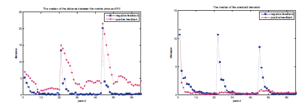
Figure 12: Positive/Negative Feedback; Large Shocks Coordination & Price Discovery; median absolute distance to RE fundamental price; median standard deviation of individual predictions
Figure 12 consist of two line graphs that graph distance versus period. Both graphs contain a pink line representing positive feedback and a blue line representing negative feedback.  The left graph, with an x-axis that goes from 0 to 70 and a y-axis that goes from 0 to 25, shows the median of the distance between the market price and RE.  The right graph, with an x-axis that goes from 0 to 70 and a y-axis that goes from 0 to 15, shows the median of the standard deviation.

In the left graph, both lines follow the same general path, though the pink line is consistently above the blue line by about 2 to 5.  The pink line starts at 7 and the blue line starts at 5. Both lines fall to near 0 at period 9. The blue line bumps along 0 until 20 periods in, whereas the pink line gradually increases to about 2.5 over this stretch.  Then both lines increase rapidly - the pink line to 15 and the blue line to 13, before dropping down again. The blue line falls to 0 again at 25 periods and stays there until 44, whereas the pink line stays around 4. At 42 periods both lines again shoot upward, the pink line to 22 and the blue line to 20. They fall back down again, the blue line to 0 where it stays for the remainder of the graph, and the pink line to around 3. The pink line has as small bump back up to 5 before declining again to 3, before jumping up to 4 in the last period.

In the right graph, the pink line starts at 12 and falls sharply to almost zero within the first 3 periods, and bumps along the x-axis until 45 periods when it increases to 2 and then falls down to 1 for the remainder of the graph. The blue line starts at 11 and then falls to 1 in the first 10 periods, where it remains until 22 periods when it jumps back up to 12, before falling to 1 again by period 27. It stays at 1 again until period 4 when it jumps to 9, then falls back to 1 by period 51, and stays there for the remainder of the graph.

Bao et al. (2010) recently ran similar LtFEs with large permanent shocks  \epsilon_t to the price generating mechanisms (6.1) and (6.2). These shocks have been chosen such that, both in the negative and positive feedback treatments, the fundamental equilibrium price  p^* changes over time according to:

\begin{displaymath}\begin{array}{lll} p_t^* &= & 56 \hskip2.5cm 0\leq t \leq 21 \\ p_t^* &= & 41 \hskip2.5cm 22\leq t \leq 43 \\ p_t^* &= & 62 \hskip2.5cm 44\leq t \leq 65. \end{array}\end{displaymath} (6.3)

The purpose of these experiments was to investigate how the type of expectations feedback may affect the speed of learning of a new steady state equilibrium price. Figure 11 shows realized market prices together with the simulated market prices (left panels), together with the evolution of the fractions of the four strategies of the heuristics switching model (right panels) for a typical group of the negative feedback (top panels) and the positive feedback treatment (bottom panels). The heuristics switching model is exactly the same as in Anufriev and Hommes (2009), in the case of the asset pricing experiments (see Section 5), with the same benchmark parameters as before, i.e.  \beta=0.4, \eta=0.7, \delta= 0.9. As in the case of small shocks, there is a striking difference between positive and negative feedback markets. In the negative feedback market, after each large shock the price quickly (within 5 periods) settles down to the RE benchmark, while in the positive feedback market the price slowly oscillates with persistent deviations from the RE benchmark. The heuristics switching model matches both patterns quite nicely and provides an intuitive, behavioral explanation why these different aggregate patterns occur. In the negative feedback market, trend following strategies perform poorly and the adaptive expectations strategy quickly dominates the market (more than  50\% within 10 periods) enforcing quick convergence to the RE benchmark after each large shock. In contrast, in the positive feedback treatment, trend following strategies perform well, the weak trend following rule dominates in the first 20 periods, while the strong trend following rule starts dominating after the first large shock in period 22.

Figure 12 reveals some other striking features of aggregate price behavior and individual forecasts. The left panel shows the time variation of the median distance to the RE benchmark price over all groups in both treatments. For the negative feedback treatment, after each large shock the distance spikes but converges quickly back (within 5-6 periods) to 0, while for the positive feedback treatment after each shock the distance to the RE benchmark shows a similar spike but does not converge to 0 and only decreases slowly. The right panel shows how the degree of heterogeneity, that is, the median standard deviation of individual forecasts, changes over time. For the positive feedback treatment after each large shock heterogeneity decreases very quickly and converges to (almost) 0 within 3-4 periods, while in the negative treatment heterogeneity is more persistent for about 10 periods after each large shock. One may summarize these results in saying that in the positive feedback treatment individuals quickly coordinate on a common prediction, but that coordination on the "wrong" non-fundamental price occurs. On the other hand, in the negative feedback treatment coordination is slow, heterogeneity is more persistent but price convergence is quick. Stated differently, positive feedback markets are characterized by quick coordination and slow price discovery, while negative feedback markets are characterized by slow coordination, more persistent heterogeneity and quick price discovery. See Bao et al. (2009) for a more detailed discussion.


7 A New Keynesian Macro Model

As a final example, we briefly discuss the LtFEs experiments in a standard New Keynesian macro model of Assenza et al. (2009); see also Pfajfar and Santoro (2009) for closely related LtFEs. The New Keynesian model is described by the following equations:

\displaystyle y_{t} \displaystyle = \displaystyle y_{t+1}^{e}-\varphi(i_{t}-\pi_{t+1}^{e})+g_{t}\,, (7.1)
\displaystyle \pi_{t} \displaystyle = \displaystyle \lambda y_{t}+\beta\pi_{t+1}^{e}+u_{t}\,, (7.2)
\displaystyle i_{t} \displaystyle = \displaystyle \phi_{\pi}(\pi_{t}-\overline{\pi})+\overline{\pi}\,, (7.3)

where  y_{t} and  y_{t+1}^{e} are respectively the actual and the expected output gap at time  t,  i_{t} is the nominal interest rate,  \pi_{t} and  \pi _{t+1}^{e} are respectively the actual and expected inflation rates,  \overline{\pi} is the target inflation rate,  \lambda,  \sigma,  \beta and  \varphi are positive coefficients, and  g_{t} and  u_{t} are (small) white noise shocks. The coefficient  \phi_{\pi} measures the response of the nominal interest rate  i_{t} to changes in the inflation rate  \pi_{t}. Equation (7.1) is the IS curve in which the actual output gap  y_{t} depends on the expected output gap  y_{t+1}^{e} and on the real interest rate  i_{t}-\pi_{t+1}^{e}. Equation (7.2) is the expectations-augmented New Keynesian Phillips curve according to which actual inflation depends on the actual output gap and expected inflation. Finally, equation (7.3) is the monetary policy rule implemented by the Central Bank in order to keep inflation at its target level  \overline{\pi}.

In the LtFEs of Assenza et al. (2009), two different groups of 6 subjects have to provide two-period ahead forecasts of the inflation rate respectively the output gap for 50 periods. Realized inflation and realized output gap are determined by the (average) individual expectations of two different groups of 6 individuals. Subjects only obtain qualitative information about the macro-economy, but they do not know the underlying law of motion (7.1-7.3).

Figure 13: Learning to forecast experiment in New Keynesian Macro framework. Left panel: time series of realized inflation, individual inflation forecasts, interest rate and realized output gap. Right panel: time series of realized inflation, interest rate, realized output gap and individual forecasts of output gap. Parameter values:  \phi _{\pi }=1.5, ...

Figure 13 has two line graphs. The left graph is labeled Tr 3b gr2 infl. And has a y-axis that goes from -1.5 5o 5.5 and a x-axis that goes from 0 to 50.  The second graph is labeled Tr 3b gr2 output gap and has a y-axis that runs from -2 to 5 and an x-axis that also runs from 0 to 50.  In both graphs there are three lines labeled in the legend: the inflation rate is black, the output gap is orange, and the interest rate is purple.  Those three lines have identical paths in both graphs.  However, there are other lines that are not labeled (they are brown, yellow, blue and pink) that change from graph to graph.  In the first graph, they mainly follow the path of the purple line, with some noise, and in the second graph they mainly follow the orange line, again with some noise. In both graphs, there are two horizontal black dashed lines at the y-values of 2 and 0.25.  The orange line starts at 0.25 and then decreases to -0.5 before oscillating around 0 with decreased amplitude until the end of the graph.  The purple and black lines follow similar paths, starting at 4 and 3 respectively, where they decrease and then oscillate around about 2.25 with decreased amplitude.

Figure 14: New Keynesian Macro Model: Simulations of heuristics switching model

Figure 14: New Keynesian Macro Model: Simulations of Heuristics switching model
Figure 14 has four line graphs in a two-by-two formation.  The top two graphs have a red line for the simulation and a blue scatter points for the experiment, and both graphs have an x-axis that runs from 0 to 50 periods.  In the bottom two graphs, there are four lines: a blue line which represents ADA, a red line with represents WTR, a black line which represents STR, and a green line that represents LAA.   Both of the bottom graphs have an x-axis that runs from 0 to 50 periods and y-axes that run from 0 to 1.

The top left graph represents output and has a y-axis that runs from -1.5 to 1.5.  The red line starts at 0.3 and then sharply drops to -1 in the first 4 periods.  It then jumps up to 0.75, before falling again. For the next two wavelengths the amplitude increases around the median of about 0.25, and then the amplitude decreases as the wave oscillates between about 0.5 and -1 from periods 25 to 40. After period 40, the wave's amplitude is severely dampened to about 0.1 and the median increases from less than 0 to just above 0. Throughout the graph, the blue scatter plot closely matches the red line.

In the bottom left graph, all the lines start at the same value of 0.25 and remain there for the first 4 periods.  Then the black line steadily decreases (with decreasing slope) until it reaches a minimum of 0 at 42 periods in. It then rises slightly to end the graph at 0.5.  The purple line similarly decreases after four periods, running just below the black line until 35 periods in when it starts to increase. It reaches a maximum of 0.5 at 42 periods and then declines ever so slightly to end the graph at 0.45.  The red line stays around 0.25 until 10 periods in, when it starts to decline slightly faster than the black and purple lines, so it appears they are converging. However, before they intersect the red line starts to increase again, and increases with a pretty steady rate to end the graph at 0.25.  The green line starts to increase after 4 periods and reaches a maximum at 0.85 23 periods in. It then slopes down again, crosses the purple line at 40 periods in and starts to flatten out at the end of the graph, ending just below 0.3.

The top right graph represents inflation and has a y-axis that runs from 1 to 4.  The red line starts at 4 and sharply drops down to 1.5. From there it oscillates with decreasing amplitude about 2.25 until period 33 when its amplitude is dampened to about 0.5 and it oscillates irregularly around 2.  Throughout the graph the blue scatter plot is fit very well around the red line.

In the bottom right graph, all the lines start at the same value of 0.25 and remain there for the first 4 periods.  Then the black line increases to 0.4 before decreasing with increasing slope until it reaches a minimum of just above 0 at 36 periods in. From there it rises to end the graph just below 0.1.  The purple line starts to decrease after period 4 and reaches a minimum of just above 0 at 24 periods in, before rising at a moderate right and ending the graph just below 0.4.  The red line has a small dip right after 4 periods to 0.2 before it has a small bump to 0.3 at 10 periods in, where it then decreases to reach a minimum of 0.124 periods in. From there it rises to end the graph at 0.3.  The green line has a small dip to 0.2 at 9 periods in before rising to a maximum at 0.8. From there it falls steadily to end the graph at 0.275

Figure 13 shows time series of realized inflation, output gap, interest rate together with individual forecasts of inflation and output gap. Both inflation and output gap exhibit dampened oscillations eventually converging to the RE benchmark steady state. An interesting feature of these experiments is that an aggressive monetary policy described by a Taylor type interest rate rule that adjust the interest rate more than one point for one in response to inflation (with a coefficient  \phi _{\pi }=1.5) is able to stabilize heterogeneous expectations.

Figure 14 shows simulated time series of inflation and output gap, together with the fractions of the forecasting rules, of the benchmark heuristics switching model of Anufriev and Hommes (2009). The same heuristics switching model is used for both inflation and output gap forecasts and the model fits the experimental data quite well. The patterns of the weight of the forecasting heuristics are quite similar for inflation and output, as one would expect since both time series are qualitatively similar. The Learning Anchor and Adjustment (LAA) rule dominates most of the time, with a peak of about  80\% after 25 periods and the adaptive expectations rule dominating in the last 10 periods when the economy stabilizes. There is a slight difference in the initial phase, with the strong trend rule STR dominating inflation forecasting in periods 5-10, picking up the stronger trend in inflation.

8 Concluding Remarks

LtFEs can be used to test theories of expectations and learning in benchmark model settings. LtFEs are Taylor made experiments to test exclusively the expectations hypothesis, computerizing all other model assumptions. Different outcomes in aggregate behavior have been observed in different market settings. To our best knowledge, no homogeneous expectations model fits all LtFEs across different settings. Quick convergence to the RE-benchmark only occurs in stable (i.e. stable under naive expectations) cobweb/negative feedback markets.

Lab experiments suggest that heterogeneity is a crucial aspect of a theory of expectations, because a heterogeneous expectations model can explain observed path dependence in the same market environment as well as different aggregate outcomes across different market settings.

A challenge to economic theory is to come up with a universal and plausible theory of heterogeneous expectations. The fact that a simple heuristics switching model fits different LtFEs gives some hope that a general heterogeneous expectations hypothesis may explain individual expectations and aggregate outcomes across different market settings.
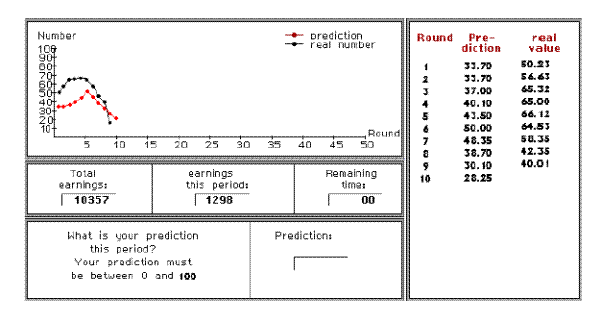
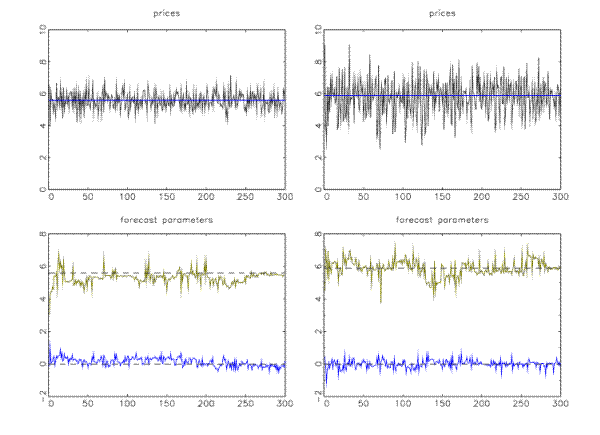
Bibliography

Adam, K., (2007),
Experimental evidence on the persistence of output and inflation, The Economic Journal 117 (520) , 603-636 .
Akerlof, G.A. and Shiller, R.J., (2009),
Animal Spirits: How Human Psychology Drives the Economy, and Why It Matters for Global Capitalism, Princeton University Press.
Allen and Taylor, (1990),
Charts, noise and fundamentals in the London foreign exchange market, Economic Journal 100, No. 400, Conference Papers, 49-59.
Anderson, E.W., Ghysels, E. and Juergens, J.L., (2005),
Do heterogeneous beliefs matter for asset pricing? Review of Financial Studies 18, 875-924.
Anufriev, M. and Hommes, C. , (2009),
Evolutionary Selection of Individual Expectations and Aggregate Outcomes, CeNDEF Working Paper 09-09, University of Amsterdam, September 2009.
Arifovic, Jasmina., 1994.
"Genetic algorithm learning and the cobweb model." Journal of Economic Dynamics and Control 18(1): 3-28.
Baak, S.J., (1999),
Tests for bounded rationality with a linear dynamic model distorted by heterogeneous expectations, Journal of Economic Dynamics and Control 23, 1517-1543.
Bao, T., Hommes, C.H., Sonnemans, J. and Tuinstra, J., (2010),
Individual expectation, limited rationality and aggregate outcome, CeNDEF working paper, January 2010.
Barberis, N. and Thaler, R., (2003),
A survey of behavioral finance, Handbook of the Economics of Finance, In: Constantinidis, G.M. et al. (Eds.), Elsevier.
Basak, S., (2000),
A model of dynamic equilibrium asset pricing with heterogeneous beliefs and extraneous risk, Journal of Economic Dynamics and Control 24, 63-95.
Bénassy-Quéré, Larribeau, S. and MacDonald, R., (2003),
Models of exchange rate expectations: how much heterogeneity?, International Financial Markets, Institutions and Money 13, 113-136.
Benartzi, S. and Thaler, R.H., (2007),
Heuristics and biases in retirement savings behavior, Journal of Economic Perspectives 21, 81-104.
Boswijk, H.P., Hommes, C.H. and Manzan, S., (2007),
Behavioral heterogeneity in stock prices, Journal of Economic Dynamics and Control 31, 1938-1970.
Bottazzi, G., Devetag, G. and Pancotto, F., (2008),
Does Volatility matter? Expectations of price return and variability in an asset pricing experiment, CEEL Working Paper 1-08.
Branch, W.A., (2004),
The theory of rationally heterogeneous expectations: evidence from survey data on inflation expectations, Economic J. 114, 592-621.
Branch, W.A., (2007),
Sticky information and model uncertainty in survey data on inflation expectations, Journal of Economic Dynamics and Control 31
Branch, W.A. and Evans, G.W., (2006),
Intrinsic heterogeneity in expectation formation, Journal of Economic Theory 127, 264-295.
Brock, W.A. and Hommes, C.H., (1997),
A rational route to randomness, Econometrica 65, 1059-1095.
Brock, W.A., and Hommes, C.H., (1998),
Heterogeneous beliefs and routes to chaos in a simple asset pricing model, J. Econ. Dyn. & Contr. 22, 1235-1274.
Camerer, C.F. and Ho, T.H., (1999),
Experienced-weighted attraction learning in normal form games, Econometrica 67, 827-874.
Campbell, J.Y., A.W. Lo and A.C. MacKinlay, (1997),
The Econometrics of Financial Markets, Princeton University Press, Princeton.
Capistrán, C. and Timmermann, A., (2009),
Disagreement and biases in inflation expectations, Journal of Money, Credit and Banking 41, 365-396.
Carlson, J., (1967),
The stability of an experimental market with a supply response lag, Southern Economic Journal 33, 305–321.
Chavas, J.P., (2000)
On information and market dynamics: the case of the U.S. beef market, Journal of Economic Dynamics and Control 24, 833-853.
Chiarella, C., R. Dieci and X. He, (2009),
Heterogeneity, market mechanisms, and asset price dynamics, In: Hens, T. and K. R. Schenk-Hoppé (Eds.), Handbook of Financial Markets: Dynamics and Evolution, Elsevier, pp. 277-344.
Colander, D., Föllmer, H., Haas, A., Goldberg, M.D., Juselius, K., Kirman, A. Lux, T. and Sloth, B., (2009)
. The Financial Crisis and the Systemic Failure of Academic Economics, Univ. of Copenhagen Dept. of Economics Discussion Paper No. 09-03. Available at SSRN: http://ssrn.com/abstract=1355882
Colucci, D. and Valori, V., (2006),
Ways of learning in a simple economic setting: a comparison, Chaos, Solitons and Fractals 29, 653-670.
DeGrauwe, P., (2009),
What's wrong with modern macroeconomics. Top-down versu bottom-up macroeconomics, CESifo Economic Studies Conference Paper, November 2009.
Delli-Gatti, D., Gaffeo, E., Gallegati, M., Giulioni, G. and Pallestrini, A., (2008),
Emergent macroeconomics. An agent-based approach to business fluctuations, Springer Verlag, Milan.
DeLong, J.B., Shleifer, A., Summers, L.H. and Waldmann, R.J., (1990),
Noise trader risk in financial markets, Journal of Political Economy 98, 703-738.
Diks, C.G.H. and Weide, R. van der, (2005),
Herding, A-synchronous Updating and Heterogeneity in Memory in a CBS, Journal of Economic Dynamics and Control 29, 741-763.
Dreger, C. and Stadtmann, G., (2008),
What drives heterogeneity in foreign exchange rate expectations: insights from a new survey, International Journal of Finance and Economics 13, 360-367.
Duffy, J., (2006),
Agent-based models and human-subject experiments, in Leigh Tesfatsion and Kenneth L. Judd (ed.), Handbook of Computational Economics, edition 1, volume 2, chapter 19, pages 949-1011.
Duffy, J. (2008a),
Experimental Macroeconomics, Entry in: S. Durlauf and L. Blume, (Eds.), The New Palgrave Dictionary of Economics, 2nd ed., New York: Palgrave Macmillan.
Duffy, J. (2008b),
Macroeconomics: a survey of laboratory research, In: J. Kagel A.E. Rot, (Eds.), Handbook of Experimental Economics, Volume 2, forthcoming.
Ellen, ter S. and Zwinkels, R.C.J., (2009),
Oil price dynamics: a behavioral finance approach with heterogeneous agents, Working Paper, Erasmus University Rotterdam.
Elliott, G. and Ito, T., (1999),
Heterogeneous expectations and tests of efficiency in the yen/dollar forward exchange rate market, Journal of Monetary Economics 43, 435-456.
Erev, I. and Roth, A.E., (1998),
Prediction how people play games: reinforcement learning in games with unique strategy equilibrium, American Economic Review 88, 848-881.
Evans, G.W. and Honkapohja, S, (2001),
Learning and expectations in macroeconomics, Princeton University Press, Princeton.
Farmer, J.D. and Geanakoplos, J., (2009),
The virtures and vices of equilibrium and the future of financial economics, Complexity 14, 11-38.
Fehr, E. and Tyran, J.-R., (2001),
Does money illusion matter? American Economic Review 91, 1239-1262.
Fehr, E. and Tyran, J.-R., (2005),
Individual irrationality and aggregate outcomes, Journal of Economic Perspectives 19, 43-66.
Fehr, E. and Tyran, J.-R., (2008),
Limited rationality and strategic interaction: the impact of the strategic environment on nominal inertia, Econometrica 76, 353-394.
Frankel, J.A. and Froot, K.A., (1987)
Short-term and Long-term Expectations of the Yen/Dollar Exchange Rate: Evidence from Survey Data, Journal of the Japanese and International Economies 1, 249-274; also published as NBER working paper 2216, April 1987.
Frankel, J.A. and Froot, K.A., (1990)
The Rationality of the Foreign Exchange Rate. Chartists, Fundamentalists and Trading in the Foreign Exchange Market, American Economic Review 80, no. 2, AEA Papers and Proceedings, 181-185.
Grandmont, J.-M., (1998),
Expectation formation and stability in large socio-economic systems, Econometrica 66, 741-781.
Haruvy, E., Lahav, Y. and Noussair, C.N., (2007),
Traders' expectations in asset markets: experimental evidence, American Economic Review 97, 1901-1920.
Heemeijer, P., Hommes, C.H., Sonnemans, J. and Tuinstra, J., (2009),
Price stability and volatility in markets with positive and negative expectations feedback, Journal of Economic Dynamics & Control, 1052-1072.
Hens, T. and Schenk-Hoppé, K.R. (Eds.), (2009),
Handbook of Financial Markets: Dynamics and Evolution, Elsevier.
Holt, C.A. and A.P. Villamil, (1986),
A laboratory experiment with a single person cobweb, Atlantic Economic Journal 14, 51–54.
Hommes, C.H., (2006),
Heterogeneous agent models in economics and finance, In: Tesfatsion, L. and Judd, K.L., (eds), Handbook of Computational Economics, Volume 2: Agent-Based Comp. Econ., chapter 23, North-Holland, 1109-1186.
Hommes, C.H., (2009),
Bounded Rationality and Learning in Complex Markets, In: Handbook of Economic Complexity, Edited by J. Barkley Rosser, Jr., Cheltenham: Edward Elgar.
Hommes, C.H., Huang, H. and Wang, D. (2005b),
A robust rational route to randomness in a simple asset pricing model. Journal of Economic Dynamics and Control 29, 1043-1072.
Hommes, C.H. and Lux, T., (2009),
Individual Expectations and Aggregate Behavior in Learning to Forecast Experiments, CeNDEF Working Paper, University of Amsterdam.
Hommes, C.H., Sonnemans, J., Tuinstra, J., and van de Velden, H., (2005a)
Coordination of expectations in asset pricing experiments, Review of Financial Studies 18, 955-980.
Hommes, C., J. Sonnemans, J. Tuinstra and H. van de Velden, (2007),
Learning in cobweb experiments, Macroeconomic Dynamics 11 (S1), 8-33.
Hommes, C.H., Sonnemans, J., Tuinstra, J. and Velden, H. van de, (2008),
Expectations and bubbles in asset pricing experiments, Journal of Economic Behavior & Organization 67, 116-133.
Hommes, C.H., J. Sonnemans and H. van de Velden, (2000),
Expectation formation in an experimental cobweb economy, In: D. Delli Gatti, M. Gallegati and A. Kirman (eds.). Interaction and Market Structure: Essays on Heterogeneity in Economics, Lecture Notes in Economics and Mathematical Systems, volume 484, pp. 253–266. Berlin: Springer-Verlag
Hommes, C. H., and Sorger, G., (1998)
Consistent Expectations Equilibria, Macroeconomic Dynamics 2, 287-321.
Hommes, C.H. and Wagener, F.O.O., (2009),
Complex Evolutionary Systems in Behavioral Finance, In: T. Hens and K.R. Schenk-Hoppé (Eds.), Handbook of Financial Markets: Dynamics and Evolution, Elsevier, 2009, 217-276.
Jong, de E., Verschoor, W.F.C. and Zwinkels, R.C.J., (2009),
Behavioural heterogeneity and shift-contagion: Evidence from the Asian crisis, Journal of Economic Dynamics and Control 33, 1929-1944.
Kelley, H. and D. Friedman, 2002
, Learning to Forecast Price, Economic Inquiry, 40, 556-573.
LeBaron, B., (2006),
Agent-based Computational Finance, Handbook of Computational Economics, Volume 2: Agent-Based Computational Economics, chapter 24, L. Tesfatsion and K.L. Judd (Eds.), North-Holland, Amsterdam, 1187-1233.
Lei, V., Noussair, C.N. ad Plott, C.R., (2001),
Nonspeculative bubbles in experimental asset markets: lack of common knowledge of rationality vs. actual irrationality, Econometrica 69, 831-859.
Lillo, F., Moro, E., Vaglica, G. and Mantegna, R.N., (2008),
Specialization and herding behavior of trading firms in a financial market, New Journal of Physics 10, 043019.
Lucas, R.E., (1972),
Econometric testing of the natural rate hypothesis, In: O. Eckstein (ed.) The econometrics of price determination Conference. Board of Governors of the Federal Reserve System and Social Science Research Council, Washington DC, 1972, 50-59.
Lucas, R.E., (1986),
Adaptive behavior and economic theory, Journal of Business 59 (4), S401-S426.
Lux, T., (2009)
Stochastic behavioral asset pricing models and the stylized facts, In: T. Hens and K.R. Schenk-Hoppé (Eds.), Handbook of Financial Markets: Dynamics and Evolution, Elsevier, 2009.
MacDonald, R. and Marsh, I., (1996),
Currency forecasters are heterogeneous: confirmation and consequences, Journal of International Money and Finance 15, 665-685.
Mankiw, N.G., Reis, R., Wolfers, J., (2003),
Disagreement about inflation expectations, In: Gertler, M., Rogoff, K. (Eds.), NBER Macroeconomics Annual 2003.
Marimon, R., S.E. Spear and S. Sunder, 1993
, Expectationally Driven Market Volatility: an Experimental Study, Journal of Economic Theory, 61, 74-103.
Marimon, R. and S. Sunder, (1993),
Indeterminacy of Equilibria in a Hyperinflationary World: Experimental Evidence, Econometrica 61, 1073-1107.
Marimon, R. and S. Sunder, (1994),
Expectations and Learning under Alternative Monetary regimes: an experimental approach, Economic Theory 4, 131-162.
Marimon, R. and S. Sunder, (1995),
Does a constant money growth rule help stabilize inflation? Carnegie-Rochester Conference Series on Public Policy 43, 111-156.
Menkhoff, L and Taylor, M.P., (2007),
The obstinate passion of foreign exchange professionals: technical analysis, Journal of Economic Literature 45, 936-972.
Muth, J.F., (1961)
Rational expectations and the theory of price movements, Econometrica 29, 315-335.
Pesaran, H.M. and Weale, M., (2006),
Survey expectations, In: G. Elliott, C.W.J. Granger and A. Timmermann, Handbook of Economic Forecasting, Amsterdam, North-Holland, pp.715-76.
Plot, C.R. and S. Sunder, (1982),
Efficiency of experimental security markets with insider information: an application of rational expectations models, Journal of Political Economy 90, 663-698.
Rosser, J. Barkley, (2009),
Handbook of Economic Complexity, Jr., Cheltenham: Edward Elgar.
Sargent, T.J. (1993):
Bounded rationality in macroeconomics, Clarendon Press.
Sargent, T.J. (2008),
Evolution and intelligent design, American Economic Review 98, 5-37.
Schmalensee, R., 1976,
An Experimental Study of Expectation Formation, Econometrica, 44, 17-41.
Schunk, D., (2009),
Behavioral heterogeneity in dynamic search situations: Theory and experimental evidence, Journal of Economic Dynamics and Control 33, 1719-1738.
Shefrin, H. and Statman, M., (1994),
Behavioral capital asset pricing theory, The Journal of Financial and Quantitative Analysis 29, 323-349.
Shiller, R.J., 2000,
Measuring bubble expectations and investor confidence, Journal of Psychology and Financial Markets 1, 49-60.
Simon, H.A., (1957),
Models of man, Wiley, New York, NY.
Sims, C.A., (1980),
Macroeconomics and reality, Econometrica 48, 1-48.
Smith, V.L., (1962),
A experimetal stud of competitive market beavior, Joural of Political Ecoom 70, 111-137.
Smith, V.L., G.L. Suchanek and A.W. Williams, 1988,
Bubbles, Crashes and Endogenous Expectations in Experimental Spot Asset Markets, Econometrica, 56, 1119-1151.
Sunder, S.,
Experimental asset markets: a survey: In: J.H. Kagel and A.E. Roth, (Eds.), Handbook of Experimental Economics, Princeton University Press, 445-500.
Sutan, A. and Willinger, M., (2009),
Guessing with negative feedback: An experiment, Journal of Economic Dynamics and Control 33, 1123-1133.
Taylor, M.P. and Allen, H., (1992),
The use of technical analysis in the foreign exchange market, Journal of International Money and Finance 11, 304-314.
Tesfatison, L. and Judd, K.L., (eds), 2006,
Handbook of Computational Economics, Volume 2: Agent-Based Comp. Econ., North-Holland.
Tversky, A. and Kahneman, D., (1974),
Judgment under uncertainty: heuristics and biases, Science 185, 1124-1131.
van de Velden, H., (2001),
An Experimental Approach to Expectation Formation in Dynamic Economic Systems, Ph-D Dissertation, Tinbergen Institute Research Series 268.
Williams, A.W., (1987)
The Formation of Price Forecasts in Experimental Markets, Journal of Money, Credit and Banking, 19, 1-18.
Vaglica, G., Lillo, F., Moro, E. and Mantegna, R.N., (2008),
Scaling laws of strategic behavior and size heterogeneity in agent dynamics, Physical Review E 77, 036110.
Vissing-Jorgensen, A., (2003),
Perspective on behavioral finance: does `irrationality' disappear with wealth? Evidence from expectations and actions, In: Gertler, M., Rogoff, K. (Eds.) NBER Macroeconomics Annual, MIT Press.
Wellford, C.P., (1989),
A Laboratory Analysis of Price Dynamics and Expectations in the Cobweb Model, Discussion Paper No. 89-15, Department of Economics, University of Arizona
Williams, J., (1977),
Capital asset prices with heterogeneous beliefs, Journal of Financial Economics 5, 219-239.
Zapatero, F., (1998),
Effects of financial innovation on market volatility when beliefs are heterogeneous, Journal of Economic Dynamics and Control 22, 597-626.


Footnotes

* This work was presented at a plenary lecture at the 15th International Conference on Computing in Economics and Finance (CEF), Sydney, July 15-17, 2009. I would like to thank the participants of the CEF-conference for many stimulating discussions. This survey is based on longlasting cooperation and many ideas from my co-authors Joep Sonnemans, Jan Tuinstra, Henk van de Velden, Peter Heemeijer, Buz Brock and Tiziana Assenza and particularly benefitted from ideas, simulations and figures provided by Mikhail Anufriev, Te Bao, Domenico Massaro and Thomas Lux. Financial support from the EU 7th framework collaborative project Monetary, Fiscal and Structural Policies with Heterogeneous Agents (POLHIA), grant no. 225408, is gratefully acknowledged. None of the above are responsible for errors in this paper. Return to Text
1. There is also an extensive literature on heterogeneous belief models based on heterogeneous information, see e.g. Williams (1977), Shefrin and Statmann (1994), Zapatero (1998), Basak (2000) and Anderson et al. (2005). Return to Text
2. 1300 points corresponded to 0.5 Euro, so that maximum earnings were 25 Euro's. Average earnings ranged from 11.5 to 21 Euro (in about 1.5 hours), over the different treatments. Return to Text
3. Colucci and Valori (2006) fit simple adaptive learning rules to the individual cobweb LtFE of Hommes et al. (2000). Arifovic (1994) calibrates a GA-learning model to the cobweb experiments of Wellford (1989). Return to Text
4. See Hommes and Sorger (1998), where the parameters of an AR1 rule are updated according to sample autocorrelation learning. Return to Text
5. In similar cobweb LtFE experiments Heemeijer et al. (2009) recently estimated individual forecasting rules, and many individuals actually used forecasting rules of the simple AR1-form (3.7). Return to Text
6. Gaunersdorfer (2000) studies the case with time varying beliefs about variances and Chiarella and He (2002,2003) investigate the model with heterogeneous risk aversion coefficients. Return to Text
7. Bottazzi et al. (2008) consider asset pricing LtFEs were, in addition to a price forecast subjects must also forecast the variance of excess returns, which is then used in the mean-variance demand function (4.3) to compute the market clearing price. Return to Text
8. In the experiment  n_t never exceeds 0.25, while the weight of the other traders are equal to  (1- n_t)/6. Hommes et al. (2008) investigate price behavior in asset pricing LtFEs without robot traders. Return to Text
9. At this stage one could argue that the anchor of this rule, defined as the average between the last observed price and the fundamental price, was unknown in the experiment, since subjects were not provided explicitly with the fundamental price. It is remarkable however that for a number of subjects the linear estimated forecasting rule was surprisingly close to the anchor and adjustment rule (4.9) Return to Text
10. Price dynamics in group 3 (not shown, but see the concluding remarks) is more difficult to classify. Similar to group  1 it started with moderate oscillations, then stabilized at a level below the fundamental, suddenly falling in period  t=40, probably due to a typing error of one of the participants. Return to Text
11. The heuristics switching model is similar to other models of reinforcement learning, e.g. Erev and Roth (1998) and Camerer and Ho (1999). An important difference however is that our model is built in a market environment rather than the strategic environments usually studied in standard game theory. Schunk (2009) introduces a dynamic model of behavioral heterogeneity in search behavior and shows that his experimental data is well explained by a model assuming dynamic updating of utility reference points. Return to Text
12. Haruvy et al. (2007) also provide experimental evidence that individual price expectations are significantly affected by past price trends. Trend following behavior is often associated with technical trading strategies in real financial markets; see Menkhoff and Taylor for a comprehensive overview of the importance of technical analysis. Return to Text
13. These values have been obtained in Anufriev and Hommes (2009) after some trial and error simulations. The simulation results however are fairly robust with respect to small changes in these parameter values. Return to Text
14. In both treatments, the absolute value of the slopes is 0.95, implying in both cases that the feedback system is stable under naive expectations Return to Text

This version is optimized for use by screen readers. Descriptions for all mathematical expressions are provided in LaTex format. A printable pdf version is available. Return to Text