Skip to: [Printable Version (PDF)] [Bibliography] [Footnotes]

Finance and Economics Discussion Series: 2006-28 Screen Reader version*

The U.S. Treasury Yield Curve:

1961 to the Present^*

Refet S. Gürkaynak

Brian Sack

and

Jonathan H. Wright^**

June 2006

Keywords: Yield curve, forward rates, on-the-run premium, treasury market

Abstract:

The discount function, which determines the value of all future nominal payments, is the most basic building block of finance and is usually inferred from the Treasury yield curve. It is therefore surprising that researchers and practitioners do not have available to them a long history of high-frequency yield curve estimates. This paper fills that void by making public the Treasury yield curve estimates of the Federal Reserve Board at a daily frequency from 1961 to the present. We use a well-known and simple smoothing method that is shown to fit the data very well. The resulting estimates can be used to compute yields or forward rates for any horizon. We hope that the data, which are posted on the website http://www.federalreserve.gov/pubs/feds/2006 and which will be updated periodically, will provide a benchmark yield curve that will be useful to applied economists.

 

1. Introduction

The U.S. Treasury yield curve is of tremendous importance both in concept and in practice. From a conceptual perspective, the yield curve determines the value that investors place today on nominal payments at all future dates--a fundamental determinant of almost all asset prices and economic decisions. From a practical perspective, the U.S. Treasury market is one of the largest and most liquid markets in the global financial system. In part because of this liquidity, U.S. Treasuries are extensively used to manage interest rate risk, to hedge other interest rate exposures, and to provide a benchmark for the pricing of other assets.

With these important functions in mind, this paper takes up the issue of properly measuring the U.S. Treasury yield curve. The yield curve that we measure is an off-the-run Treasury yield curve based on a large set of outstanding Treasury notes and bonds. We present daily estimates of the yield curve from 1961 to 2006 for the entire maturity range spanned by outstanding Treasury securities. The resulting yield curve can be expressed in terms of zero-coupon yields, par yields, instantaneous forward rates, or -by- forward rates (that is, the -year rate beginning years ahead) for any and .

Section 2 of the paper reviews all of these fundamental concepts of the yield curve and demonstrates how they are related to each other. Section 3 describes the specific methodology that we employ to estimate the yield curve, and Section 4 discusses our data and some of the details of the estimation. Section 5 shows the results of our estimation, including an assessment of the fit of the curve, and section 6 demonstrates how the estimated yield curve can be used to calculate the yield on "synthetic" Treasury securities with any desired maturity date and coupon rate. As an application of this approach, we create a synthetic off-the-run Treasury security that exactly replicates the payments of the on-the-run ten-year Treasury note, allowing us accurately to measure the liquidity premium on that issue. Section 7 offers some concluding thoughts. The data are posted as an appendix to the paper on the FEDS website.

2. Basic Definitions

This section begins by reviewing the fundamental concepts of the yield curve, including the necessary "bond math." It then describes the specific estimation method employed in this paper.

2.1 The Discount Function and Zero-Coupon Yields

The starting point for pricing any fixed-income asset is the discount function, or the price of a zero-coupon bond. This represents the value today to an investor of a $1 nominal payment years hence. We denote this as . The continuously compounded yield on this zero-coupon bond can be written as

$$y_t (n)=-\ln (d_t (n))/n,$$ (1)

and conversely the discount function can be written in terms of the yield as

$$d_t (n)=\exp (-y_t (n)n).$$ (2)

Although the continuously compounded basis may be the simplest way to express yields, a widely used convention is to instead express yields on a "coupon-equivalent" or "bond-equivalent" basis, in which case the compounding is assumed to be semi-annual instead of continuous. For zero-coupon securities, this involves writing the discount function as

$$d_t (n)=\frac{1}{(1+y_t^{ce} /2)^{2n}},$$ (3)

where is the coupon-equivalent yield. One can easily verify that the continuously compounded yield and the coupon-equivalent yield are related to each other by the following formula:

$$y_t =2\ln (1+y_t^{ce} /2).$$ (4)

Thus, it is easy to move back and forth between continuously compounded and coupon-equivalent yields.

The yield curve shows the yields across a variety of maturities. Conceptually, the easiest way to express the curve is in terms of zero-coupon yields (either on a continuously compounded basis or a bond-equivalent basis). However, practitioners instead usually focus on coupon-bearing bonds.

2.2 The Par-Yield Curve

Given the discount function, it is straightforward to price any coupon-bearing bond by summing the value of its individual payments. For example, the price of a coupon-bearing bond that matures in exactly years (paying $1) is as follows:

$$P_t (n)=\sum\limits_{i=1}^{2n} {(c/2)d_t (i/2)+d_t (n)} ,$$ (5)

where is the semi-annual coupon payment on the security--that is, it has a stated annual coupon rate of .³ Of course, for coupon-bearing bonds the yield will depend on the coupon rates that are assumed.

One popular way to express the yields on coupon-bearing bonds is through the concept of par yields. A par yield for a particular maturity is the coupon rate at which a security with that maturity would trade at par (and hence have a coupon-equivalent yield equal to that coupon rate). The yield can be determined from an equation similar to (5), only setting the price of the security equal to $1:

$$1=\sum\limits_{i=1}^{2n} {\frac{y_t^p (n)}{2}d_t (i/2)+d_t (n)} ,$$ (6)

where we have replaced the coupon rate with the variable to denote the -year par yield. Solving equation (6), the par yield is then given by:⁴

$$y_t^p (n)=\frac{2(1-d_t (n))}{\sum\limits_{i=1}^{2n} {d_t (i/2)} }.$$ (7)

The par yields from equation (7) are expressed on a coupon-equivalent basis. A continuously compounded version of this can be derived by assuming a bond pays out a continuous coupon rate, in which case the par yield with maturity , , is given by:

$$y_t^{p,cc} (n)=\frac{1-d_t (n)}{\int_0^n {d_t (i)di} }.$$ (8)

Zero-coupon yields are a mathematically simpler and more fundamental concept than par yields. However, one advantage of expressing the yield curve in terms of par yields is that financial market participants typically quote the yields on coupon-bearing bonds. Most financial commentary focuses on individual Treasury securities, most often the on-the-run issues--the most recently issued securities at each maturity. These securities trade near par (at least initially) and have shorter duration (owing to the positive coupon) than zero-coupon yields with the same maturities.⁵ Of course, the choice of whether to focus on zero-coupon yields or par yields is simply a choice of the manner to present the yield curve once estimated; these are alternative ways of summarizing the information in the discount function. In fact, the yield curve can be used to compute the yield for a security with any specified coupon rate and maturity date--an approach that we will use below to analyze individual securities.

2.3 Forward Rates

The yield curve can also be expressed in terms of forward rates rather than yields. A forward rate is the yield that an investor would agree to today to make an investment over a specified period in the future--for -years beginning years hence. These forward rates can be synthesized from the yield curve. Suppose that an investor buys one -year zero-coupon bond and sells -year zero-coupon bonds. Consider the cash flow of this investor. Today, the investor pays for the bond being bought and receives for the bond being sold. These cash flows, of course, cancel out, so the strategy does not cost the investor anything today. After years, the investor must pay as the -year bond matures. After a further years, the investor receives $1 as the -year bond matures. Thus, this investor has effectively arranged today to buy an -year zero-coupon bond years hence. The (continuously compounded) return on that investment, determined by the amount that the investor must pay at time to receive the $1 payment at time , is what we will refer to as the -by- forward rate, or the -year rate beginning years hence. The forward rate is given by the following formula:

$$f_t (n,m)=-\frac{1}{m}\ln (\frac{d_t (n+m)}{d_t (n)})=\frac{1}{m}\left( {(n+m)y_t (n+m)-ny_t (n)} \right),$$ (9)

with the last equality following from (2). Taking the limit of (9) as goes to zero gives the instantaneous forward rate years ahead, which represents the instantaneous return for a future date that an investor would demand today:

$$f_t (n,0)=\lim _{m\to 0} f_t (n,m)=y_t (n)+n{y}'_t (n)=-\frac{\partial }{\partial n}\ln (d_t (n)),$$ (10)

where the last equality again uses equation (2). Notice that (10) implies that the yield curve is upward (downward) sloping whenever the instantaneous forward rate is above (below) the zero-coupon yield at a given maturity.

One can think of a term investment today as a string of forward rate agreements over the horizon of the investment, and the yield therefore has to equal the average of those forward rates. Specifically, from equation (10), , and so, from equation (2), the -period zero-coupon yield (expressed on a continuously compounded basis) is given by:

$$y_t (n)=\frac{1}{n}\int_0^n {f_t (x,0)dx} .$$ (11)

Likewise we can write as the average of one-year continuously compounded forward rates:

$$y_t (n)=\frac{1}{n}\Sigma _{i=1}^n f_t (i-1,1).$$ (12)

Thus, given a complete range of forward rates, one can calculate the complete yield curve from equations (11) and (12), or, conversely, given the complete yield curve, one can calculate all the forward rates from equations (9) and (10). Yields and forward rates are simply alternative ways of describing the same curve.

By using forward rates, we can summarize the yield curve in some potentially more informative ways. For example, the ten-year Treasury yield can be decomposed into one-year forward rates over that ten-year horizon. As we will discuss below, near-term forward rates tend to be affected by monetary policy expectations and hence cyclical variables, while longer-term forwards instead are determined by factors seen as more persistent or by changes in risk preferences. The ten-year yield meshes these two types of influences together, whereas it may be easier to interpret that yield when one considers the near-term and distant forward rates separately. Indeed, former Fed Chairman Greenspan often parsed the yield curve into its various forward components (see for example his February and July 2005 Monetary Policy Testimonies). Similarly, Gürkaynak, Sack, and Swanson (2005) frame their discussion of the responsiveness of the yield curve to macroeconomic news in terms of forward rates, pointing to the fact that distant forward rates appear to respond to incoming data (which they associate with movements in long-term inflation expectations).

Lastly, one can also compute forward rates for future investments that have coupon payments. A par forward rate is the coupon rate that one would demand today to make a $1 investment at time and to receive back $1 in principal at time along with semiannual coupons from time n+ to time , assuming that and are coupon dates. Let denote this -by- par forward rate (expressed with semiannual compounding). An investor can synthesize this par forward rate agreement by selling one -year zero coupon bond and buying of -year zero-coupon bonds and one more year zero-coupon bond, where is set so as to ensure that the net cash flow today is zero. This implies that

$$d_t (n)-\Sigma _{i=1}^{2m} d_t (n+i/2)\frac{f_t^p (n,m)}{2}-d_t (n+m)=0.$$ (13)

Solving this equation gives the formula for the -by- par forward rate:

$$f_t^p (n,m)=\frac{2(d_t (n)-d_t (n+m))}{\sum\limits_{i=1}^{2m} {d_t (n+i/2)} }.$$ (14)

Whereas continuously compounded zero-coupon yields can be written as the average of the corresponding continuously compounded forward rates, as in equations (11) and (12), we cannot simply write par yields as averages of the constituent par forward rates. However, Campbell, Lo and Mackinlay (1997) and Shiller, Campbell and Schoenholtz (1983) show, using a loglinear approximation, that

$$y_t^p (n)\approx \frac{1-\rho }{1-\rho ^n}\Sigma _{i=1}^n \rho ^if_t^p (i-1,1),$$ (15)

where , the analog of equation (12) for par rates.

2.4 Duration and Convexity

Before moving on to yield curve modeling and estimation, we introduce a couple of key concepts for the yield curve: duration and convexity.

Duration is a fundamental concept in fixed-income analysis. Much of the value of a coupon-bearing security comes from coupon payments that are being made before maturity, so the effective time that investors must wait to receive their money is shorter than the maturity of the bond. The Macaulay duration of a bond is a weighted average of the time that the investor must wait to receive the cash flows on a coupon-bearing bond (in years):

$$D=\frac{1}{P_t (n)}[\sum\limits_{i=1}^{2n} {\frac{i}{2}\frac{c}{2}d_t (i/2)+nd_t (n)} ].$$ (16)

Zero-coupon bonds have duration equal to the maturity of the bond, but coupon-bearing securities have shorter duration. For a given maturity, the higher the coupon rate is, the shorter the duration.

Closely related to this concept is the modified duration of a bond, , which is defined as the Macaulay duration divided by one plus the yield on the bond (assuming semi-annual compounding):

$$D_{MOD} =\frac{D}{1+\textstyle{{y^{ce}} \over 2}}.$$ (17)

It can be shown that the derivative of the log price of a bond with respect to its yield is simply . Thus, modified duration provides the sensitivity (in percent) of the value of a bond to small changes in its yield.

A related concept is that of convexity. Modified duration measures the sensitivity of the log price of a bond to changes in yield, but it is accurate only for small changes in yield. The reason it is not accurate for large changes in yield is that the relationship between prices and yields is nonlinear: the capital gain induced by a decline in the yield is larger than the capital loss induced by an equal-sized increase in the yield.

Convexity captures this nonlinearity. To a second-order approximation, the change in the log price of the bond is given by:

$$d\log (P)=-D_{\bmod } dy+\frac{1}{2}\kappa (dy)^2,$$ (18)

where is the convexity of the bond. Convexity has implications for the shape of the yield curve that will be an important consideration in the choice of our methodology for estimating the yield curve.

In particular, convexity tends to pull down longer-term yields and forward rates, an effect that increases with uncertainty about changes in yields. Consider, for example, an increase in the uncertainty about a long-term interest rate that is symmetric in terms of the possible basis-point increase or decrease in yield. For a given level of the yield, this tends to increase the expected one-period return on the bond because of the asymmetry noted above--that the capital gain from a fall in the yield is greater than the capital loss from a rise in the yield. Formally, consider the expected value of the -period zero-coupon bond one period ahead, which we can write as . By Jensen's inequality, we have:

$$E_t [d_{t+1} (n)]=E_t [\exp (-y_{t+1} (n)n)]>\exp (E_t [-y_{t+1} (n)]n).$$ (19)

In other words, the expected value is higher than the value that would be associated with the expected yield next period.

Markets, of course, recognize this effect and incorporate it into the pricing of the yield curve. In particular, the convexity effect tends to push down yields, as investors recognize the boost to expected return from the convexity term and hence are willing to pay more for a given bond. This effect tends to be larger for bonds with longer maturities, giving the yield curve a hump shape that is discussed at greater length below.

3. Yield Curve Estimation

If the Treasury issued a full spectrum of zero coupon securities every day, then we could simply observe the yield curve and have a complete set of the yields and forward rates described in the previous section. That, unfortunately, is not the case. Treasury has instead issued a limited number of securities with different maturities and coupons. Hence, we usually have to infer what the yields would be across the maturity spectrum from the prices of existing securities.

For each date, we know the prices (and therefore yields) of a number of Treasury securities with different maturities and coupon payments. Accounting for the differences in maturities and coupons is not a problem; the estimation will simply view coupon-bearing bonds as baskets of zero-coupon securities, one for each coupon payment and the principal payment (as described above).⁶ The more significant problem is the fact that we do not have securities at all maturities. To come up with yields across the complete maturity spectrum, we have to interpolate between the existing securities. This exercise is what constitutes yield curve estimation.

In embarking on this exercise, one is immediately confronted by an important issue: how much flexibility to allow in the yield curve. Put differently, one has to decide whether all observed prices of Treasury securities exactly reflect the same underlying discount function. This is surely not the case: Idiosyncratic issues arise for specific securities, such as liquidity premia, hedging demand, demand for deliverability into futures contracts, or repo market specialness (which is often related to the other factors). Moreover, some variation across securities could arise from bid-ask spreads and nonsynchronous quote times, though we believe that these effects are quite small in our data (described below).

In any case, it is desirable (and in fact necessary) to impose some structure on the yield curve to smooth through some of this idiosyncratic variation. However, one can choose different methods that vary in terms of how much flexibility is allowed. One can estimate a very flexible yield curve which would fit well in terms of pricing the existing securities correctly, but do so with considerable variability in the forward rates. Or, one could impose more smoothness on the shape of the forward rates while sacrificing some of the fit of the curve. The more flexible approaches tend to be spline-based methods that involve a large number of estimated parameters, while the more rigid methods tend to be parametric forms that involve a smaller number of parameters.

The choice in this dimension depends on the purpose that the yield curve is intended to serve. A trader looking for small pricing anomalies may be very concerned with how a specific security is priced relative to those securities immediately around it. Suppose, for example, that the yield curve has a dip in forward rates beginning, say, in year eight that is associated with the fact that securities in that sector are the cheapest-to-deliver into the Treasury futures contract (an example we will show below). The trader, in assessing the value of an individual security in that sector, would probably want to incorporate that factor into his relative value assessment, and hence he would want to use a yield curve flexible enough to capture this variation in the forwards. By contrast, a macroeconomist may be more interested in understanding the fundamental determinants of the yield curve. Because it is difficult to envision a macroeconomic factor that would produce a brief dip in the forward rate curve eight years ahead, he may wish to use a more rigid yield curve that smoothes through such variation.

Our primary purpose in estimating the yield curve is to understand its fundamental determinants such as macroeconomic conditions, monetary policy prospects, perceived risks, and investors' risk preferences. Considering this purpose, we will employ a parametric yield curve specification. As will be seen below, this specification will allow for very rich shapes of the forward curve while largely ruling out variation resulting from a small number of securities at a given maturity.

Our approach follows the extension by Svensson (1994) of the functional form that was initially proposed by Nelson and Siegel (1987). The Nelson-Siegel approach assumes that instantaneous forward rates years ahead are characterized by a continuous function with only four parameters:

$$f_t (n,0)=\beta _0 +\beta _1 \exp (-n/\tau _1 )+\beta _2 (n/\tau _1 )\exp (-n/\tau _1 ).$$ (20)

With this function, instantaneous forward rates begin at horizon zero at the level and eventually asymptote to the level . In between, forward rates can have a "hump," with the magnitude and sign of the hump determined by the parameter and the location of the hump determined by the parameter .

Below we will show some results that allow us to interpret the shape of the forwards that result from this functional form. But at this point, it is worth making a few notes. We can always interpret forward rates as having two components: expected future short-term interest rates and a term premium. Under Nelson-Siegel, the forward rates will tend to start at the current short-term rate that is largely determined by the current monetary policy setting (the starting point), will be governed at intermediate-horizons by expectations of the business cycle, inflation, and corresponding monetary policy decisions (the hump), and will end up at a steady-state level (the asymptote).

It turns out, however, that this yield curve has difficulty fitting the entire term structure, especially those securities with maturities of twenty years or more. The reason is convexity. As discussed in section 2 above, convexity tends to pull down the yields on longer-term securities, giving the yield curve a concave shape at longer maturities (as will be seen below). The Nelson-Siegel specification, while fitting shorter maturities quite well, tends to have the forward rates asymptote too quickly to be able to capture the convexity effects at longer maturities.

For that reason, we instead use the more flexible approach described in Svensson (1994). This approach assumes that the forward rates are governed by six parameters according to the following functional form:

$$f_t (n,0)=\beta _0 +\beta _1 \exp (-n/\tau _1 )+\beta _2 (n/\tau _1 )\exp (-n/\tau _1 )+\beta _3 (n/\tau _2 )\exp (-n/\tau _2 ).$$ (21)

In effect, this specification adds two new parameters (the last term in the equation) that allow a second "hump" in the forward rate curve. The yield curve collapses to Nelson-Siegel when is set to zero. However, as we will see below, the yield curve typically needs a second hump, one that usually occurs at long maturities, to capture the convexity effects in the yield curve. Integrating these forward rates gives us the corresponding zero-coupon yields:

$$y_t (n)=\beta _0 +\beta _1 \frac{1-\exp (-\frac{n}{\tau _1 })}{\frac{n}{\tau _1 }}+\beta _2 [\frac{1-\exp (-\frac{n}{\tau _1 })}{\frac{n}{\tau _1 }}-\exp (-\frac{n}{\tau _1 })]+\beta _3 [\frac{1-\exp (-\frac{n}{\tau _2 })}{\frac{n}{\tau _2 }}-\exp (-\frac{n}{\tau _2 })],$$ (22)

and from these yields one can compute the discount function at any horizon.

Thus, for a given set of parameters, the Svensson specification characterizes the yield curve and discount function at all maturities. The discount function can then be used to price any outstanding Treasury security with specific coupon rates and maturity dates. In estimating the yield curve, we choose the parameters to minimize the weighted sum of the squared deviations between the actual prices of Treasury securities and the predicted prices. The weights chosen are the inverse of the duration of each individual security. To a rough approximation, the deviation between the actual and predicted prices of an individual security will equal its duration multiplied by the deviation between the actual and predicted yields. Thus, this procedure is approximately equal to minimizing the (unweighted) sum of the squared deviations between the actual and predicted yields on all of the securities.

Of course, this is just one of many specifications that we could have chosen. A number of other papers instead use spline-based methods, including Fisher, Nychka, and Zervos (1995), Waggoner (1997), and McCulloch (1975, 1990). These methods generally allow for more variation in the forward rate curve (though the degree of flexibility can be controlled in the specifications). However, that flexibility may come with some costs. Bliss (1996) compares a number of estimation methods and finds that parsimonious specifications such as the Nelson-Siegel method perform favorably relative to some of the more flexible methods. In addition, Sack (2000) demonstrates some of the estimation difficulties that can arise under more flexible approaches for estimating the U.S. term structure.

4. Data and Estimation Issues

We employ the Svensson methodology for estimating our benchmark yield curve. In our view, this method strikes an appealing balance between being flexible enough to fit the U.S. yield curve well and being parsimonious enough to avoid over-fitting the idiosyncratic variation in the yields of individual securities. As described above, we estimate the six parameters, using maximum likelihood, to minimize the sum of the squared deviations between the actual prices of Treasury securities and the predicted prices, where the prices are weighted by the inverse of the duration of the securities.

Our underlying quotes on Treasury securities come from two primary sources. For the period from 14 June 1961 to the end of November 1987, we rely on the CRSP daily Treasury file, which provides end-of-day quotes on all outstanding Treasury securities. Since December 1987, we use Treasury quotes provided by the Federal Reserve Bank of New York (FRBNY), which is a proprietary database constructed from several sources of market information.⁷

An immediate issue that arises is determining the set of securities to be included in the estimation. The Treasury securities outstanding at any point in time can differ in many dimensions, including their liquidity and their callable features. Our goal is to use a set of securities that are similar in terms of their liquidity and that do not have special features (such as being callable) that would affect their prices. In other words, we would ideally have securities that only differ in terms of their coupons and maturities.

To that end, we include in the estimation all outstanding Treasury notes and bonds, with the following exceptions:

(i) We exclude all securities with option-like features, including callable bonds and flower bonds.⁸

(ii) We exclude all securities with less than three months to maturity, since the yields on these securities often seem to behave oddly. This behavior may partly reflect the lack of liquidity for those issues and segmented demand for short-term securities by particular investor classes.

(iii) We also exclude all Treasury bills out of concern about segmented markets. Indeed, Duffee (1996) showed that bill rates are often disconnected from the rest of the Treasury yield curve, perhaps owing to segmented demand from money market funds and other short-term investors.

(iv) We begin to exclude twenty-year bonds in 1996, because those securities often appeared cheap relative to ten-year notes with comparable duration. This cheapness could reflect their lower liquidity or the fact that their high coupon rates made them unattractive to hold for tax-related reasons.⁹

(v) We exclude the two most recently issued securities with maturities of two, three, four, five, seven, ten, twenty, and thirty years for securities issued in 1980 or later. These are the "on-the-run" and "first off-the-run" issues that often trade at a premium to other Treasury securities, owing to their greater liquidity and their frequent specialness in the repo market.¹⁰ Earlier in the sample, the concept of an on-the-run issue was not well defined, since the Treasury did not conduct regular auctions and the repo market was not well developed (as discussed by Garbade (2004)). Our cut-off point for excluding on-the-run and first off-the-run issues is somewhat arbitrary but is a conservative choice (in the sense of potentially erring on the side of being too early).

(vi) Other issues that we judgmentally exclude on an ad hoc basis. For example, there were large and persistent fails-to-deliver in the May 2013 3? percent ten-year note, well after it ceased to be either the on-the-run or first off-the-run ten-year security. With the security persistently trading around the fails rate in the overnight repo market, the yield on the security in the cash market was driven down. Thus, we dropped the security for some time to avoid having our yield curve distorted by the idiosyncratic dislocation of this issue.

These restrictions imply that we are estimating an "off-the-run" Treasury yield curve, one for which the liquidity of the included securities should be relatively uniform. The liquidity implicit in our curve should be regarded as adequate, though far short of the remarkable liquidity of on-the-run issues.

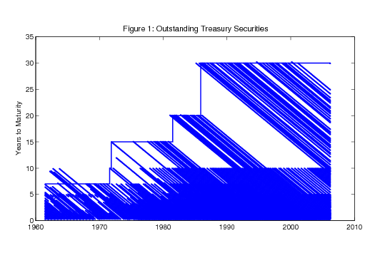
The ranges of maturities available for estimation over our sample are shown graphically in Figure 1, which takes the same form as a figure reported by Bliss (1996). The date is shown on the horizontal axis, the remaining maturity is shown on the vertical axis, and each outstanding Treasury coupon security is represented by a dot showing its remaining maturity on that date. For example, a dot at a ten-year maturity in 1985 denotes a security that is to mature ten years later, in 1995. That same security will be represented by a dot at the nine-year maturity in 1986.

In the results below, we report estimates of the yield curve at horizons that go as far out as possible without extrapolating far beyond the range of maturities that are actually outstanding. The maximum maturity that we report is shown by the horizontal line segments in Figure 1. Specifically, we report yield curve estimates out to seven years for the early part of the sample, extend them to ten years on 16 August 1971, to fifteen years on 15 November 1971, to twenty years on 2 July 1981, and to thirty years since 25 November 1985.¹¹ Of course, with the estimated parameters from the Svensson yield curve, one could compute yields and forward rates at any horizon; however, we would strongly recommend only focusing on those measures at the horizons for which outstanding securities were available for estimation.

A final issue is whether to make adjustments for tax effects, a topic discussed by McCulloch (1975). In our view, the correct adjustment is difficult to determine, in part because Treasury securities are held by a wide range of investors with different tax brackets. In fact, a large set of Treasury investors, including pension funds and others, are exempt from taxes. Moreover, Treasury securities provide a tax advantage on state and local taxes that depends on the state of residence of the investor. Given these considerations, we chose not to make adjustments for tax effects. Nevertheless, tax considerations may be important in some applications, in which case users might want to make tax adjustments to our smoothed yield curve.

5. Results

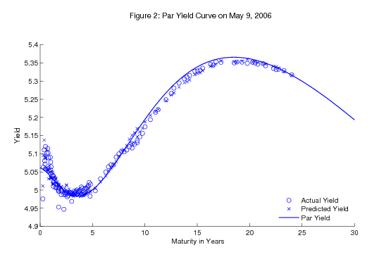
Using the above methodology, we estimate the U.S. Treasury yield curve from June 1961 to the present. As an example of the results, Figure 2 shows the estimated yield curve on May 9, 2006. The solid line is the continuously compounded par yield curve, the open circles are the actual quotes on all outstanding coupon securities included in the estimation, and the crosses are the predicted yields for those issues.

As can be seen, the yield curve does an impressive job fitting the entire cross-section of Treasury coupon issues with a function of only six parameters. The largest misses are for very short-term issues, which we attribute to the idiosyncratic nature of those securities, and for several securities in the two- to three-year maturity range that appear divorced from other yields on that day.

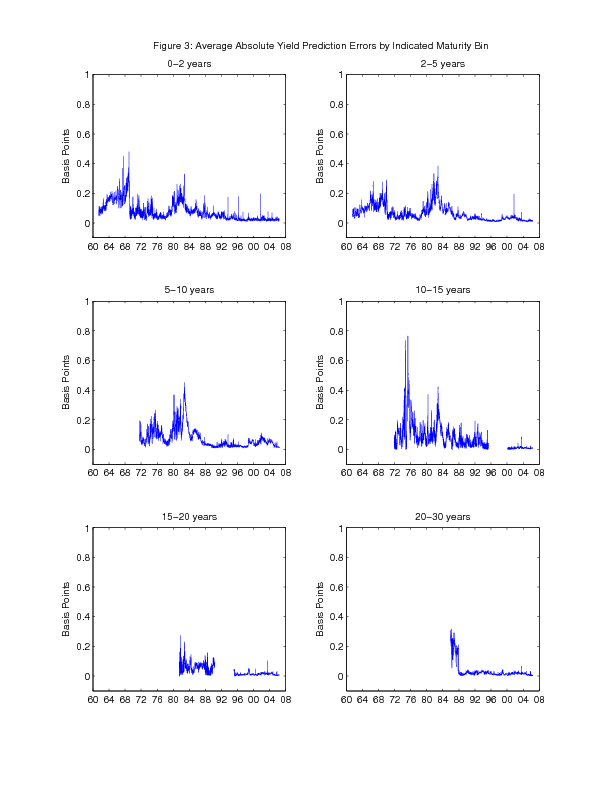
The success at fitting Treasury yields on this date is repeated throughout the sample. Figure 3 shows the average absolute yield prediction error in different maturity buckets over time. As can be seen, all of the errors are quite small over the entire sample. The largest fitting errors tend to be seen at the longest maturities that are being fitted.

In addition, the fit of the yield curve estimation has generally improved over time and is particularly good in the latter part of the sample. One possible explanation of this fact is that the market has become more active and liquid, which has reduced pricing anomalies across various securities. Under that interpretation, it is interesting to note that the fit of the estimation temporarily worsened slightly after the financial market turmoil in the fall of 1998. Fleming (2000) has suggested that Treasury securities may have become less connected to one another at that time because many of the arbitrage desks that assure the close relationships across securities became less active.

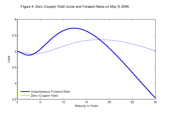
Figure 4 returns to the specific date considered in Figure 2, only now showing the instantaneous forward rates and the zero-coupon yield curve. To assess the performance of the Svensson method, it is useful to add some interpretation to the shape of the yield curve that day. At the short horizons, forward rates and yields decline slightly, apparently reflecting market expectations for slight easing of monetary policy in 2007 and beyond. Beyond this range, both curves turn up, reflecting the normal upward-sloping pattern of the yield curve associated with term premia. The upward slope of the yield curve tapers off at long horizons, however, and eventually turns down. Accordingly, the forward rates turn down earlier and much more sharply.

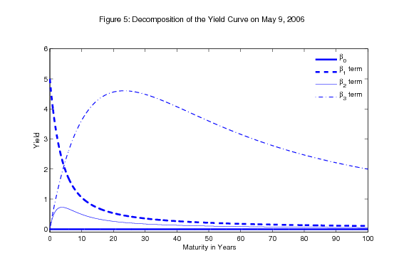
This date provides a good example of the way in which the Svensson method typically fits the U.S. yield curve. Figure 5 provides more details by showing the decomposition of this yield curve into its components on this date. Loosely speaking, as discussed in section 3, the success of this method comes from allowing two "humps" that seem to serve very different purposes. The first hump (the term) is often located at relatively short horizons, which in many cases is needed to capture the effects of near-term monetary policy expectations (along with the decay component, the term). The second hump (the term) is typically located at much longer horizons--long enough so that the forward rate schedule is still downward sloping even after 30 years, even though the specification assumes that forward rates eventually asymptote to a constant.

The downward tilt to forward rates at long horizons is an important characteristic of the U.S. yield curve; for example, the instantaneous forward rate ending 25 years ahead has continuously been below the instantaneous forward rate ending 20 years ahead for the past decade. This pattern most likely reflects the convexity of longer-term securities, which pulls down their yields for the reasons discussed above.¹²

The asymptote for the forward rate curve (the term) is estimated to be zero on this date, which arises because the convexity effect leaves forward rates sloping downward at the longest maturities and there are no perpetuities issued by the Treasury to accurately pin down the infinite horizon yield. For this reason, the asymptote is usually not strongly identified and is estimated to be zero at times. As was seen in Figure 2, this underidentification of the asymptote has no implications for the fit of the yield curve over the range of existing maturities.

Because the second hump is typically located at such long horizons, it cannot be reliably identified in the earlier parts of our sample, when the longest maturity available was fifteen, ten, or even seven years. This consideration forces us to impose some restrictions on the estimation method earlier in our sample. Specifically, we use the Nelson-Siegel specification for the period before 1980; put differently, we restrict the parameter to be zero. This is a restriction that probably would not hold if longer-term securities were available over that period, but imposing it does not significantly affect the fit of the yield curve at the short maturities available.

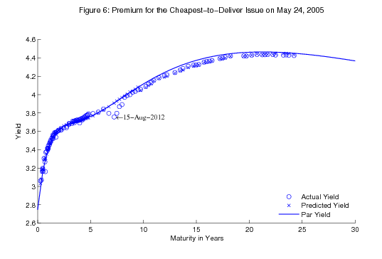
While the Svensson specification is sufficiently rich to capture the shape of the yield curve associated with policy expectations and convexity, it is not so flexible as to be significantly influenced by the idiosyncratic behavior of a small number of securities. A useful example took place in the spring of 2005, when the markets reportedly became concerned that the supply of ten-year notes that were cheapest-to-deliver into the Chicago Board of Trade's Treasury futures contract was not sufficient to meet the required delivery (Whitehouse, Lucchetti and McKay (2005)). As shown in Figure 6, the market began to place a significant premium on the August 2012 note, which was cheapest-to-deliver into the June 2005 ten-year futures contract. Those securities immediately surrounding this issue also attracted a premium. Some fitting methods would capture this pattern with sizable swings in forward rates about seven years ahead that are unrelated to macroeconomic fundamentals. The Svensson yield curve, however, is rigid enough that it does not give a dip at that particular maturity, but instead fits the general shape of the yield curve.

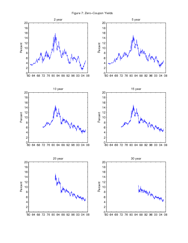
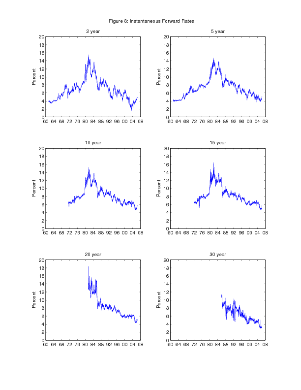
One important advantage of our yield curve estimates is that they are available over a long history. The full history of estimates for a selected set of Treasury yields and forward rates is shown in Figures 7 and 8. Yields and forward rates generally drifted higher over the late 1960s and 1970s and then drifted lower over most of the 1980s and 1990s, following the general pattern of inflation and longer-run inflation expectations over the sample. Of course, there is also much variation associated with the business cycle and other factors, especially at shorter maturities.

One issue that we confront when reviewing the historical yield curve estimates is that the estimated parameters demonstrate some instability, in that they sometimes jump discretely from one day to the next, often with little actual movement in underlying bond prices. Anderson and Sleath (1999) illustrate clearly that changing a single data point in the set of prices used to fit the Svensson yield curve can produce a notable shift in parameters and also in fitted yields. This is a drawback of parameterized yield curves, and forward rates can be particularly affected. However, it is important to note that although these jumps in parameters can be large, the changes in predicted yields over most of the maturity range considered are quite muted. In effect, there is an identification issue and the estimation is arriving at fairly similar yield curve shapes over the most of the maturity range considered through different combinations of parameters.¹³ This parameter instability is a drawback to the Svensson methodology, but the smoothness of the Svensson yield curve, its ease of economic interpretation, and its relative insensitivity to the parameter shifts over the range of horizons that are most relevant to monetary policymakers leads us to nonetheless prefer the Svensson curve to alternatives such as splines.¹⁴

The appendix that accompanies this paper provides data on zero-coupon yields (continuously compounded), instantaneous forward rates (continuously compounded) and par yields (coupon-equivalent) for the full range of maturities that we consider. The data are daily and are available back to June 14, 1961. The appendix also includes one-year par forward rates (coupon-equivalent) beginning one, four, and nine years ahead, as well as the estimates of the parameters of the Svensson yield curve. This appendix is posted on the website http://www.federalreserve.gov/pubs/feds/2006/200623/feds200623.xls, using the mnemonics described in Table 1. We intend to update the data regularly, as a resource for academic researchers and financial market practitioners.

We only report the yield curve at horizons for which there are outstanding Treasury securities (as discussed above). Although there is nothing to stop a researcher from constructing yields at any horizons from these parameter estimates, we strongly advise against doing so, since there is no reason to expect the extrapolation to yield reasonable results.

One maturity point for which this consideration applies is zero. The risk-free short-term interest rate (usually an instantaneous interest rate or perhaps an overnight interest rate) plays a critical role in many financial models. However, the yield curve estimated above is not designed to fit well at the very shortest maturities.¹⁵ At those maturities, the term structure of Treasury yields will be affected by factors that our parameterization will not capture, including seasonal patterns in Treasury bill issuance and the timing of FOMC meetings. Recall that we excluded all bills and those coupon securities with less than three months of remaining maturity from the estimation, partly for this reason.¹⁶

6. Synthetic Treasury Securities

There are many advantages to having a smoothed Treasury yield curve. Here we will highlight one application--the use of the yield curve to construct a "synthetic" off-the-run Treasury security with any maturity date and coupon rate desired. Such securities can be very useful for assessing the relative value of other securities.

The approach is straightforward. The estimated yield curve provides us with the value that investors place on a known, risk-free payment at any date in the future. Thus, for a hypothetical coupon rate and maturity date, we can compute the value of each payment on the security and sum them up to arrive at a predicted price of the synthetic security, which can then be converted to its yield. This represents the yield that one would expect on an off-the-run Treasury security with those exact payments.

This procedure can be used for computing a benchmark against which to measure spreads on various securities. For example, it could be applied to measure the credit risk spread for a corporate bond. Whereas most applications measure corporate spreads relative to individual Treasury securities, the payments and maturities of the two securities will differ some. By using a synthetic Treasury with identical payments, one eliminates any distortions coming from mismatched payments and the resulting differences in duration and convexity. Moreover, since it is an off-the-run synthetic Treasury security, it may have liquidity that is closer to that of the corporate bond than would an on-the-run issue.

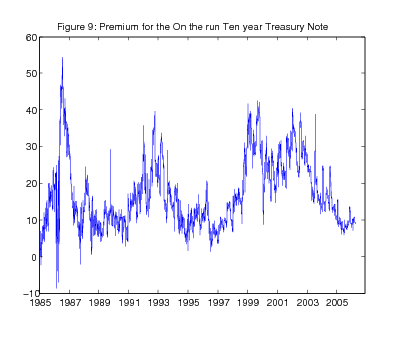
Here we choose to demonstrate this technique by considering the liquidity premium for the on-the-run ten-year Treasury note. On-the-run Treasury issues were excluded from the estimation of the yield curve. As noted above, these securities typically trade at a premium to off-the-run Treasuries, as investors are willing to pay a higher price for the greater liquidity offered by these securities. Many market participants measure the on-the-run premia relative to the first or second off-the-run security, but those issues will have shorter duration. The difference in duration can distort the measure, especially when the Treasury yield curve is steep.

We instead measure the liquidity premium for an on-the-run issue by comparing it to a synthetic off-the-run Treasury security with the same coupon rate and maturity date. The resulting measure for the ten-year Treasury note is shown in Figure 9 for the period since 1985. As can be seen, there is considerable variation in the measure at high frequency. In part, this reflects the auction pattern of the on-the-run premium: The premium tend to jump higher at the auction of a new security, when the liquidity advantage of the on-the-run issue will be realized for the longest time, and then diminishes gradually up to the auction of a new security. But there is also more gradual and persistent variation over time that is of interest. The liquidity premium appears to move up during periods of financial turmoil, including the stock market crash of 1987 and the seizing up of markets in the fall of 1998. Moreover, the premium remained relatively high from 2000 to 2002, a period during which the supply of on-the-run issues was curtailed.¹⁷ More recently, the premium has moved back to about 10 basis points, a level that appears relatively normal for tranquil periods.

The variation in this premium highlights a shortcoming of using the yields on on-the-run issues to measure of the shape of the yield curve. Movements in those yields can be associated with changes in the liquidity premium, particularly around Treasury auctions. This is why we exclude these securities from our yield curve estimation. This concern also applies to the Treasury constant maturity series (reported in the Federal Reserve's H.15 release), which are estimated from a blend of on-the-run and off-the-run issues.

7. Conclusion

In this paper we have estimated the U.S. Treasury yield curve using an approach that is simple and parsimonious. The approach is quite effective at capturing the general shape of the yield curve while smoothing through the idiosyncratic variation in the yields on individual securities. As such, the results should prove useful for understanding the general macroeconomic and other factors that have broad effects on the shape of the yield curve. The estimated yield curve can be expressed in a variety of ways, including zero-coupon yields, par yields, and forward rates.

Our yield curve fills a void in the academic literature. To our knowledge, no estimated yield curve is available on a daily basis back to the early 1960s. The dataset of Fama and Bliss (1987) (which has been updated) is monthly, and only provides estimates out to five-year maturities, while the dataset of McCulloch and Kwon (1993) is also monthly and only provides estimates out to ten-year maturities. Our data set has the advantages of being available on a daily basis, extending back to 1961, providing estimates for all maturities that are feasible given the distribution of outstanding securities, and being updated on a regular basis.

Given the importance of the yield curve in both the macroeconomics and finance literatures, we hope that our yield curve will serve as a valuable benchmark to be used in applied research. It is to this end that we have made the full dataset available to be downloaded from http://www.federalreserve.gov/pubs/feds/2006/200623/feds200623.xls and will update it regularly.

References

Anderson, Nicola and John Sleath (1999), "New Estimates of the U.K. Real and Nominal Yield Curves," Bank of England Quarterly Bulletin, November 1999, 384-392.

Bliss, Robert R. (1996), "Testing Term Structure Estimation Methods," Advances in Futures and Options Research, 9, 197-231.

Campbell, John Y., Andrew W. Lo, and A. Craig MacKinlay (1997), The Econometrics of Financial Markets, Princeton University Press, Princeton.

Duffee, Gregory (1996), "Idiosyncratic Variation of Treasury Bill Yields," Journal of Finance, 51, 527-551.

Fisher, Mark, Douglas Nychka and David Zervos (1995), "Fitting the Term Structure of Interest Rates with Smoothing Splines," Finance and Economics Discussion Series, 95-1.

Fleming, Michael J. (2000), "The Benchmark U.S. Treasury Market: Recent Performance and Possible Alternatives," Federal Reserve Bank of New York Economic Policy Review, 6, 129-145.

Garbade, Kenneth D. (2004), "The Institutionalization of Treasury Note and Bond Auctions, 1970-75," Federal Reserve Bank of New York Economic Policy Review, 10, 29-45.

Gürkaynak, Refet S., Brian Sack and Eric T. Swanson (2005), "The Sensitivity of Long-Term Interest Rates to Economic News: Evidence and Implications for Macroeconomic Models," American Economic Review, 95, 425-436.

McCulloch, J. Huston (1975), "The Tax-Adjusted Yield Curve," Journal of Finance 30, 811-830.

McCulloch, J. Huston (1990), "U.S. Term Structure Data, 1946-87," Handbook of Monetary Economics, Volume I, 672-715.

McCulloch, J. Huston and Heon-Chul Kwon (1993), "U.S. Term Structure Data, 1947-1991," Ohio State Working Paper #93-6.

Nelson, C. R. and A. F. Siegel (1987), "Parsimonious Modeling of Yield Curves," Journal of Business 60, 473-489.

Sack, Brian (2000), "Using Treasury STRIPS to Measure the Yield Curve," Finance and Economics Discussion Series Working Paper #2000-42.

Sack, Brian and Robert Elsasser (2004), "Treasury Inflation-Indexed Debt: A Review of the U.S. Experience," Federal Reserve Bank of New York Economic Policy Review 10, 47-63.

Shiller, Robert, John Y. Campbell and Kermit L. Schoenholtz (1983), "Forward Rates and Future Policy: Interpreting the Term Structure of Interest Rates," Brookings Papers on Economic Activity, 1, 173-217.

Svensson, Lars E. O. (1994), "Estimating and Interpreting Forward Rates: Sweden 1992-4," National Bureau of Economic Research Working Paper #4871.

Waggoner, Daniel (1997), "Spline Methods for Extracting Interest Rate Curves from Coupon Bond Prices," Federal Reserve Bank of Atlanta Working Paper 97-10.

Whitehouse, Mark, Aaron Lucchetti and Peter A. McKay (2005), "Short-Bond Shortage Isn't Over," Wall Street Journal, August 11, 2005.

Table 1: Description of the series in the data appendix:

Series	Compounding Convention	Mnemonics	Maturities Reported (max)
Zero-coupon yield	Continuously Comp.	SVENYXX	All integers 1-30
Par yield	Coupon-Equivalent	SVENPYXX	All integers1-30
Instantaneous forward rate	Continuously Comp.	SVENFXX	All integers 1-30
One-year forward rate	Coupon-Equivalent	SVEN1FXX	1, 4, and 9
Parameters	N/A	BETA0 to TAU2	N/A

Notes: XX in each case denotes the maturity in years. For example, SVENY10 denotes the ten-year zero-coupon yield. Maturities reported are limited before 1985 as described in the text. The one-year forward rates XX years hence denote the one-year forward rates beginning XX years hence. For example, SVEN1F09 is the one-year forward rate from nine to ten years hence. The parameters are labeled BETA0, BETA1, BETA2, BETA3, TAU1, and TAU2, corresponding to the equations in the text. Note that the parameters BETA3 and TAU2 are restricted to zero in the earlier part of the sample, as discussed in the text.

 

 

 

 

 

 

 

 

Footnotes

1. ^* We are grateful to Oliver Levine for superlative research assistance and to Brian Madigan, Vincent Reinhart and Jennifer Roush for helpful comments. All remaining errors are our own. All of the authors were involved in yield curve estimation at the Federal Reserve Board when working at that institution. The views expressed in this paper are solely the responsibility of the authors and should not be interpreted as reflecting the views of the Board of Governors of the Federal Reserve System or of any other employee of the Federal Reserve System. Return to Text

2. ^** Gürkaynak: Department of Economics, Bilkent University, 06800 Ankara, Turkey; [email protected][email protected] Sack: Macroeconomic Advisers, LLC, Washington DC 20006; [email protected] Wright: Federal Reserve Board, Washington DC 20551; (202) 452 3605; [email protected] Return to Text

3. Because the bond matures in exactly years, it is assumed to make its coupon payment today. Thus, the end-of-day price of the bond includes no accrued interest. We will have to address accrued interest in the pricing of individual Treasury securities below. Return to Text

4. For simplicity, this formula again assumes that a coupon payment has just been made and the next coupon is a full coupon period away, so that there is no accrued interest. Return to Text

5. We introduce the concept of duration in section 2.4 below. The coupon rate for an on-the-run issue is set after the auction at the highest level at which the security trades below par. Because Treasury sets coupons in increments of 12.5 basis points, this process leaves the issues trading very near par immediately after the auction. Return to Text

6. Coupon securities simply bundle together all of these individual payments. Unbundling these payments is precisely the purpose of the Treasury STRIPS program, in which each coupon and the principal can be individually traded. See Sack (2000) for an overview. Return to Text

7. We are not permitted to release either the underlying CRSP data or the FRBNY data. Return to Text

8. Flower bonds were securities with low coupons that could be redeemed at par for the payment of estate taxes. Return to Text

9. To avoid an abrupt change to the sample, we allow their weights to linearly decay from 1 to 0 over the year ending on January 2, 1996. Return to Text

10. Some simple statistics on trading volume highlight just how different the on-the-run issues are from other Treasury issues. According to Sack and Elsasser (2004), the weekly turnover rate for off-the-run Treasury securities in 2003 (that is, weekly trading volume as a percent of outstanding debt) was about 22 percent, while it was a remarkable 1400% for on-the-run issues. Return to Text

11. Note that from 1985 to 1995, there was a ten-year gap at longer maturities, reflecting the Treasury's decision to stop issuing twenty-year bonds and to start issuing thirty-year bonds in 1985. However, the yield curve estimation appears to smooth through this gap without much problem. Return to Text

12. Sack (2000) shows that this characteristic is also evident in the prices of Treasury STRIPS. Return to Text

13. For example, averaging over the days where the absolute change in was in the top percentile, the maximum absolute change in the zero-coupon yield across all maturities from one to twenty years was 10 basis points. Averaging over these days, the maximum absolute change in the instantaneous forward rate across all these maturities was 20 basis points. Meanwhile , which is the asymptote of the instantaneous forward curve jumped by over 2 percentage points on all these days. Yields, and especially forward rates, were more sensitive to these parameter jumps at maturities beyond twenty years. Return to Text

14. The instability in parameters could in principle owe to the numerical optimization algorithm for minimizing the criterion function failing to find the global minimum on some days. However, the insensitivity of our results to starting values leads us to think that this is not the case. Return to Text

15. Indeed, on a few days the extrapolated zero maturity interest rate in our dataset would even be negative. Return to Text

16. If one instead wanted to include an instantaneous or overnight interest rate, one possibility would be to use the effective federal funds rate series that is published on the Federal Reserve's H.15 data release, though some adjustment would have to be made for the small credit risk premium embedded in this rate and perhaps for its different tax treatment. Return to Text

17. The on-the-run premium has been elevated at other times as well. Indeed, the largest premium under our measure occurred in 1986. While the source of that premium is unclear, it may have been driven in part by special demand for on-the-run securities from foreign investors. Return to Text

This version is optimized for use by screen readers. A printable pdf version is available.

Home | Economic Research and Data | Accessibility | Contact us
Last update: July 11, 2008