Skip to: [Printable Version (PDF)] [Bibliography] [Footnotes]

Finance and Economics Discussion Series: 2007-07 Screen Reader version ^♣

Estimating Probabilities of Recession in Real Time Using GDP and GDI

Jeremy J. Nalewaik *

December 19, 2006

Keywords: Recessions, Markov Switching Models

Abstract:

This work estimates Markov switching models on real time data and shows that the growth rate of gross domestic income (GDI), deflated by the GDP deflator, has done a better job recognizing the start of recessions than has the growth rate of real GDP. This result suggests that placing an increased focus on GDI may be useful in assessing the current state of the economy. In addition, the paper shows that the definition of a low-growth phase in the Markov switching models has changed over the past couple of decades. The models increasingly define this phase as an extended period of around zero rather than negative growth, diverging somewhat from the traditional definition of a recession.

1 Introduction

Since Hamilton (1989, 1990), many authors have computed probabilities of recession using Markov switching models for real gross domestic product (GDP). The popularity of these models stems in part from the fact that their estimated probabilities of recession line up well with the peak and trough dates produced by the NBER's business cycle dating committee. However when Chauvet (1998), Chauvet and Piger (2002), and Chauvet and Hamilton (2005) use databases on real GDP from the Federal Reserve Bank of Philadelphia to examine the performance of Markov switching models in real time, their performance is more mixed, and was quite poor in recognizing the start of the 2001 recession. Other models have been developed to compute probabilities of recession based on dynamic factor characterizations of a host of monthly indicators such as sales, industrial production, income and employment growth. These models typically perform better than the univariate GDP model in recognizing the start of recessions, but are substantially more complicated. Further, none of these monthly indicators is as comprehensive a measure of the state of the economy as GDP.¹

Overlooked so far in this literature is the fact that, while the U.S. Bureau of Economic Analysis (BEA) press releases feature GDP, its expenditure-based estimate of the size of the economy, BEA also produces an income-based estimate of the size of the economy, gross domestic income (GDI).² GDI should equal GDP, theoretically, but in practice they often diverge substantially. The appeal of exploiting the information in GDI to date recessions is simple: it is as comprehensive as GDP, but it may capture information about the economy missed by measured GDP. For example, GDI may capture informative variation in income and employment data not fully reflected by GDP. Grimm (2005) has recently shown that GDI tends to fall more than GDP in recessions, a sign that GDI may be useful in making inferences about recessions.

This paper examines the performance of GDI for making inferences about recessions in real time. It estimates univariate Markov switching models for the growth rates of real GDI and real GDP, and bivariate Markov switching models that employ the information in both. It then compares the real time estimated probabilities of recession from these models to various benchmarks, such as the NBER start and end dates for recessions and smoothed probabilities of recession from the Markov switching models themselves.³ The main finding is that, no matter what benchmark one uses, real time GDI has done a substantially better job recognizing the start of the last several recessions than has real time GDP.

Mechanically, the main result in the paper stems in part from the fact that GDI tends to fall more than GDP in recessions, but also because the relatively small variance of GDI in the Markov switching models, conditional on the estimated state of the world, makes it more reliable than GDP as a signal of the state. In our baseline specification, the lower conditional variance is actually the key element explaining the superiority of GDI. However when we account for the mid-1980s reduction in the variance of the growth rate of the economy, the difference between mean growth rates across states becomes the more important factor.

Investigating further, the paper examines the behavior of real time probabilities estimated from the bivariate model around the start of each of the last four recessions, and shows that the corporate profits component of GDI played a particularly important role in the 2001 recession. Overall, while the examination here clearly shows that GDI has been superior in identifying the start of the last few recessions, I also point out reasons why GDP remains important to consider as well in assessing the current state of the economy.

As a secondary finding, the paper shows that the parameters estimated from the Markov switching models have changed in interesting ways over the past couple of decades. At the start of the out-of-sample evaluation period, in 1978, the models defined their low-growth state as a period with substantially negative mean growth, and their smoothed probabilities of the low-growth state lined up well with the NBER's recession dates. However, estimated mean growth in the low-growth state has crept up considerably over the past 25 years to the point where it now hovers around zero, with smoothed probabilities showing low-growth phases that are substantially longer than recessions as defined by the NBER. So it is important to note that while I continue to use the short-hand term "recession" to describe low-growth periods as identified by the models, the models are increasingly defining these periods in a way that diverges from the traditional meaning of the term. The last two recessions, with their extended periods of low growth after the nadir of the downturn - dubbed "jobless recovery" periods - seem to drive this finding. Some of these changes may stem from the acceleration of trend productivity growth since the late 1990s, which may have shifted up the mean growth rate of the economy in recession. While only the most recent recession in our sample is affected by this acceleration, it may have been significant enough to affect parameters estimated over the entire sample.

Section 2 of the paper briefly discusses the GDP and GDI data. Section 3 outlines the basic models and shows estimated probabilities of recession for the most recent quarter from 1978 to 2005 for selected BEA releases. Section 4 shows how to estimate smoothed probabilities of recession for every monthly National Income and Product Accounts (NIPA) release by BEA since 1978, and examines time series of these smoothed probabilities around the recessions in the sample. Section 5 reports results from a robustness check, showing how the results change if the basic model is altered to reflect the reduction in variance of the growth rate of the economy in the 1980's. Section 6 concludes.

2 Data: GDP and GDI

The BEA's first estimates of nominal and real GDP for the most recent full quarter are released about a month after the quarter closes; these have been called the "advance" estimates for some time now. Many components of nominal GDI come out as part of the "advance" release, but some components such as corporate profits are left missing because BEA feels that the data are not of sufficient quality for release at that time. So there is no official "advance" estimate of nominal GDI; generally we must wait until BEA's next set of estimates about a month later - called the "preliminary" estimates - to get the first read of GDI. However due to reporting lags for firms' year-end profit statements, for the fourth quarter of each year we must wait until BEA's third data release for corporate profits and GDI. The third set of estimates, inaptly named the "final" current quarterly estimates, are generally released about three months after the quarter closes.

The cycle repeats about a month after the "final" release, when the "advance" estimates for the next quarter arrive; the "final" estimates of GDP and GDI for the prior quarter generally stand until BEA conducts an annual revision. There are two exceptions to this rule for GDI, though: first, for fourth quarters up until 1993 BEA produced an additional estimate of corporate profits and GDI for quarter at the time of the "advance" quarter release, and second, since 2002 BEA has released a revised estimate of employee compensation and GDI for quarter with either the "final" or "preliminary" quarter release. The importance of this second exception will be covered in more detail when we discuss the recovery of the economy from the 2001 recession. In terms of the annual revisions, these typically occur in the summer at the time BEA releases its "advance" data for the second quarter; the NIPA data for three years prior to the current year are reopened for revision. A benchmark revision substitutes for this typical annual revision about once every five years; in a benchmark revision, data for all years are reopened for revision, and methodological changes are made as well.

Using databases maintained by BEA on the various vintages of estimates, back issues of BEA's monthly Survey of Current Business, and tables from the National Income and Product Accounts books released at the time of each benchmark revision, I constructed a real time database of the aggregates of interest. Specifically, we have at each BEA NIPA release since 1978Q1 (the "advance", "preliminary", and "final" for each quarter) what were the currently prevailing time series at that time, with the levels of each time series extending back to 1959Q3. From 1991Q4 to 2005Q3, the aggregates of interest are nominal GDP, nominal GDI, and real GDP; from 1978Q1 to 1991Q3, the aggregates of interest are nominal GNP, nominal GNI, and real GNP.⁴ We study two time series: the first, which we call , is the annualized quarterly growth rate of real GDP (or real GNP prior to 1991Q4), and the second, which we call , is the annualized quarterly growth rate of "real GDI" - nominal GDI deflated by the GDP deflator (or nominal GNI deflated by the GNP deflator prior to 1991Q4).⁵

3 Probabilities of Recession from the "Final" Current Quarterly Releases

The Basic Univariate Model

We first estimate probabilities of recession from GDP growth alone, using time series available after the "final" release for each quarter. The simple univariate model we employ is that of Chauvet and Hamilton (2005). There are two states of the world, expansion () and recession ();⁶ conditional on the state of the world, the distribution of is Gaussian,⁷ following:

The mean growth rate switches depending on the state of the economy; however each state is assumed to have a common variance .

I quickly review the recursion that produces the likelihood function and estimated probabilities of recession and expansion. Label the estimated probabilities of time expansion or recession, conditional on the history of GDP growth through time , , as:

Assume we have these probabilities in hand. We can estimate probabilities of recession and expansion next period, based on the same information set, through application of a Markov transition matrix. With two states, the Markov transition matrix contains two parameters to be estimated, and . Application of the transition matrix yields:

Given , the likelihood function for time GDP growth based on its history through time is:

We update the probability with respect to the contemporaneous as follows:

The process repeats next period. Given , this recursive procedure gives and for all periods , as well as the likelihood function to be maximized over parameters (of the Markov transition matrix and conditional densities). Smoothed probabilities that use information from the entire sample are then computed using an algorithm of Kim (1994).

Hamilton (1990) shows that the maximum likelihood parameters satisfy:

These are simple weighted averages, computed using the smoothed probabilities as weights; this result is key to the estimation procedure we employ throughout the paper, an application of the EM algorithm described in Hamilton (1990).

Before discussing the results, consider for a moment the degree to which the probabilities shift when we update them with respect to the contemporaneous growth rates. One measure of how much the probabilities shift is:

given equation (1) and the assumption of conditional normality, this reduces to:

A value closer to than to shifts the probabilities towards (and vice versa). The degree to which the probabilities shift depends on the spread between the means and the within-state variance . A larger mean spread, holding constant the conditional variance, implies more precise inferences about recessions and expansions and larger shifts in probabilities on average; a greater variance holding constant the mean spread implies smaller shifts in the probabilities. Indeed, as the variance approaches infinity, the ratio converges to one, implying no updating at all. There are two types of variance in this model, variance from the economy shifting between recessions and expansions, and within-state variation. The less of this second type, the better our inferences about the first type.

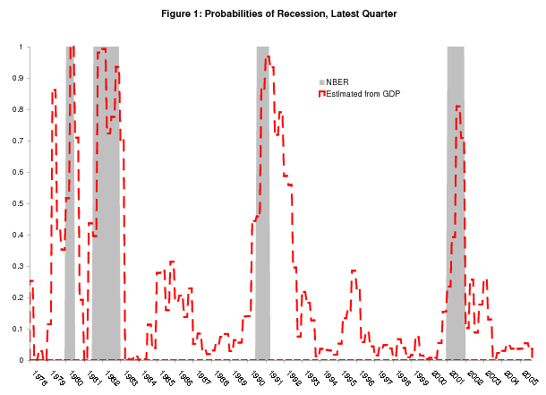
Figure 1 shows real time estimated probabilities of recession using time series back to 1959Q4 from each "final" current quarterly release from 1978Q1 to 2005Q3; the probability for the latest quarter available at each release is shown.⁸ The dashed red line shows these latest probabilities of recession estimated from the model, with recessions as defined by the NBER shaded gray.⁹ This probability shoots up well above 50% at some point during the course of each NBER recession, but in the starting quarter the signal is typically unclear. At the NBER-defined start of the 1980, 1981-82, 1990-91, and 2001 recessions, the latest probabilities were 52%, 40%, 45%, and 23%, respectively. In the latest recession, the real time performance of the model is particularly poor, giving us 23% and 39% probabilities in its first two quarters. As discussed later, and also in Chauvet and Hamilton (2005) and the 2004 Economic Report of the President, there are good reasons to believe this most recent downturn started earlier than the NBER-defined start date, which makes the performance of real GDP even poorer.

Table 1 shows the first set of parameter estimates of the model, computed using the time series of real GNP growth available in 1978Q1, and the last set of estimates, computed using the time series of real GDP growth available in 2005Q3. Standard errors are in parentheses. The last set of estimates, computed using revised data and the realizations of several additional recessions, has a slightly lower mean growth rate during expansions and a substantially higher mean growth rate during recessions, approximately equal to zero. This contraction of the mean spread , as well as the slight increase in the conditional variance , imply that it has become more difficult to recognize recessions over the last 27 years using real GDP, as its behavior in the different states has become less distinct.¹⁰ This finding is consistent with the widely reported moderation in the volatility of economic activity (e.g., McConnell and Perez-Quiros, 2000). Section 5 discusses this moderation in more detail.

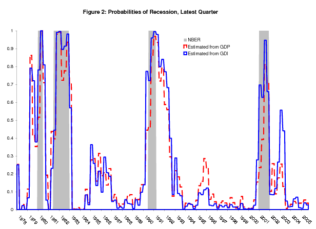
Table 2 shows the first and last parameter estimates of the same univariate model substituting real GDI, , for real GDP, . Compared to table 1, we see a slightly higher , implying a longer duration for recessions estimated from GDI, and we see a lower conditional variance for GDI, more pronounced in the last set of estimates. Figure 2 repeats the information in Figure 1, with the latest probabilities of recession estimated from GDI overlaid in solid blue. The GDI probabilities clearly perform better than the GDP probabilities at the NBER-defined start of recessions; at the starting point of the 1980, 1981-82, 1990-91, and 2001 recessions, these GDI probabilities were 78%, 44%, 72%, and 70%, respectively, each higher than the corresponding GDP probability. Some other notable features of this figure - the 1979 spike in the GDP and GDI probabilities, and the 2003 spike in the GDI probability, will be discussed later.

The Basic Bivariate Model

We next consider the bivariate generalization of the model, using both GDP and GDI to estimate probabilities of recession. We again focus on the "final" current quarterly releases, since the latest quarter's GDP and GDI are both always available with this release. The model again follows Chauvet and Hamilton (2005); GDP and GDI growth, conditional on the state of the world, are jointly normally distributed as:

so:

The Markov transition matrix is as before; the recursion that produces the likelihood function, and and for all periods , is similar to the univariate model; now denotes the history of both GDP and GDI, and the updating of with respect to and follows:

The maximum likelihood estimates of the parameters of the model satisfy:

where represent the smoothed probabilities from the bivariate model. Parameter estimates for the model are again computed via the EM algorithm.

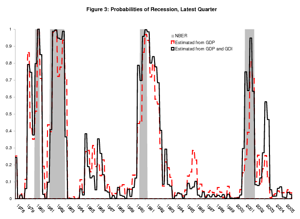
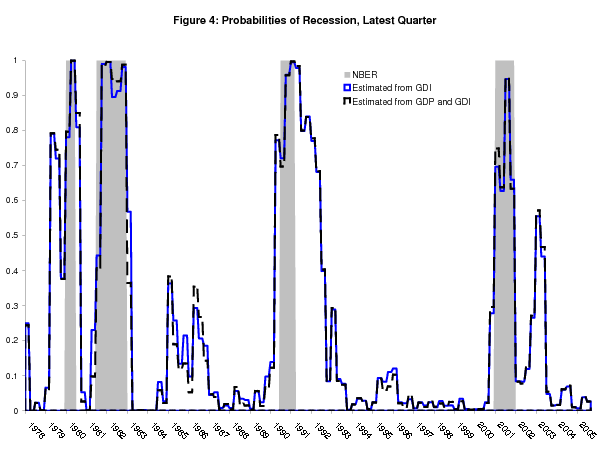
Figure 3 plots, in solid black, the real time probabilities of recession for the latest quarter from the bivariate model, along with the univariate GDP probabilities in dashed red. This figure looks very similar to Figure 2, and Figure 4 shows why: the bivariate model produces probabilities that are almost identical to the univariate GDI probabilities. So in the bivariate model, GDI dominates GDP, largely determining the probabilities of recession.

Table 3 shows the parameter estimates for the bivariate model from the first and last "final" current quarterly release we consider. In the first estimate on the 1959Q4 through 1978Q1 sample, the conditional means and variances are almost identical to those found in tables 1 and 2. Over this sample period, the model fits the 1960-61 recession, the long expansion through the 1960s, the 1969-70 recession and brief subsequent expansion, and the 1973-1975 recession and subsequent expansion. It turns out that smoothed probabilities from the univariate GDP and GDI models are quite similar over these cycles, so it is not surprising that the smoothed probabilities from the bivariate model are similar as well; equations (2) and (5) then imply the conditional means and variances of the bivariate model must be similar to those from the univariate models. For the last estimate on the 1959Q4 to 2005Q3 sample, the moments of GDI again line up with those from the univariate model, but the moments of GDP growth differ, a fact again traceable back to the smoothed probabilies: those from the bivariate model line up well with those from the univariate GDI model but differ substantially from those from the univariate GDP model in the 1980s, 1990s, and 2000s.

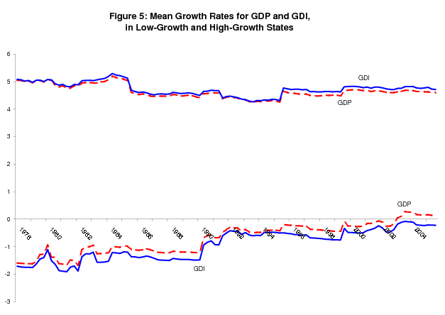
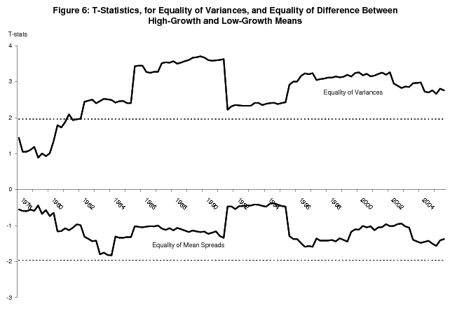
The intuition from updating formula (3) helps explain why GDI dominates in the bivariate model; the bivariate analog to this formula is more complicated, but the basic intuition is the same. A greater spread between conditional means and smaller conditional variance increases the weight a variable receives in determining the probabilities of recession and expansion. Table 3 shows that GDI wins on both counts. While figure 5 shows that the greater mean spread for GDI holds for all the intervening sets of estimates between 1978 and 2005, figure 6 shows it is never statistically significant (the line below the x-axis). However the t-statistic for the difference between the conditional variance of GDP and the conditional variance of GDI is significant at the 5% confidence level for every estimate after 1981;¹¹ the conclusion here is that the smaller conditional variance of GDI accounts for its dominance in determining probabilities of recession and expansion in the bivariate model. However, in other specifications of the model, it is the difference between the mean spreads that is key (see section 5).

As a robustness check for the result that GDI has lower conditional variance than GDP, I used smoothed probabilities from the univariate GDP model to compute the conditional moments of GDI following (2); results are shown in table 4. Standard errors reflect the fact that the smoothed probabilities are functions of parameters estimated with uncertainty - Nalewaik (2006) outlines the procedure. Comparing these results to those in tables 1 and 2, we see that, even using recession probabilites computed from GDP alone, GDI has a smaller conditional variance than GDP.

Smoothed Probabilities

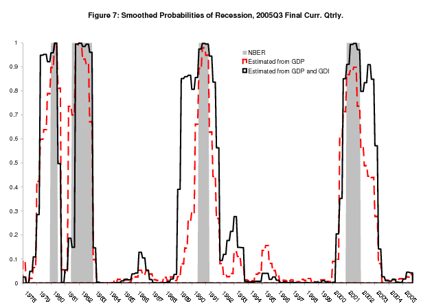
Figure 7 shows smoothed probabilities extending back to 1978 from the release of 2005Q3 "final" current quarterly data. While this figure highlights the differences between the smoothed probabilities from the bivariate model and univariate GDP model, it also highlights differences between the smoothed probabilities from the Markov switching models and the NBER recession dates. The bivariate model in particular has increasingly come to define its low-growth state as a period of mean growth around zero, including not only several quarters of negative growth strung together, but also periods of slow or around zero growth that have occured around recent contractions. For the 1980 recession, this slow growth period includes most of 1979; for the 1990-1991 recession, this slow growth period includes most of 1989 and the early part of 1990; and for the 2001 recession, this slow growth period includes 2002 and part of 2003. The GDP-based smoothed probabililities are generally closer to the NBER dates, but the movement towards a more expansive definition of the low-growth phase is evident in the univariate GDP model as well.

So we have three candidate benchmarks to which we may compare our real time estimated probabilities of recession: the NBER's dates, the latest smoothed univariate GDP probabilities, and the latest smoothed bivariate probabilities. However, no matter what benchmark one uses, the real time probabilities from the univariate GDP model do not rise fast enough at the start of recessions, a problem that is alleviated by incorporating the real time information in GDI through the bivariate model. This conclusion holds when one takes the start dates defined by the NBER as the benchmark, and Figure 7 shows that it must hold taking the smoothed probabilities as the benchmark as well, since they rise above 50% before the NBER start date for almost every recession. The only exception is the 1981-82 recession, where the smoothed bivariate probabilities suggest that the recession started in 1981Q4 rather than 1981Q3.

4 Examining Smoothed Probabilities of Recession at Each NIPA Release around Recessions

While the behavior of GDI largely determines probabilities of recession in the bivariate model, there are good reasons to avoid dropping GDP from the model altogether. One is that it is desirable to compute probabilities of recession after each "advance" and "preliminary" current quarterly NIPA release, since they are a month or two more timely than the "final" release. GDI is simply not available with the "advance" release and sometimes the "preliminary"; for these releases we must rely on GDP alone.

To deal with the unavailability of GDI in the first release or two, we estimate bivariate model parameters with data through quarter , and then employ a two stage updating procedure for inferences about , using the fact that we can factor the conditional bivariate density into a marginal and a conditional:

For releases where GDI is unavailable, we employ a first stage updating of the probabilities using the marginal densities of GDP alone:

Here denotes the the probability of expansion that has been updated with GDP alone. Appendix A derives the smoothed probabilities of recession that may be computed at this stage. In the case of full updating, the standard algorithm of Kim (1994) starts with the last probability of recession in the sample, , and iteratively produces the smoothed probabilities going back in time; so would be produced first, then , etc. In this case of partial updating, the same procedure produces the correct smoothed probabilities, but the algorithm starts with instead of . For period , the smoothing produces instead of the standard ; more generally, for any period , the smoothing produces instead of .

It is important to note that this latest probability of recession, updated with GDP alone, may look quite different from the corresponding probability from a univariate GDP model. The reason is that prior probabilities have been updated with GDP and GDI in the bivariate model, but just GDP in the univariate model, and prior probabilities have an important impact on current probabilities through the Markov transition matrix. These prior probabilities often provide critical information, in fact, as shown in some of the examples below.

Naturally, when GDI comes available in a subsequent release, the probability of recession is updated in a second stage using the density of GDI conditional on GDP:

It can be verified that, after this second stage, this procedure gives the same probabilities as are produced updating all in one stage.

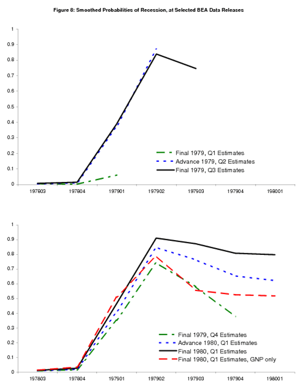
The subsections that follow undertake a closer examination of probabilities of recession at interesting NIPA release dates, examining the recent history of probabilities as well as just the latest probability. The recent history of probabilities are smoothed with the data available in real time; for example the solid black line in the top panel of Figure 8 shows the contemporaneous probability of recession for 1979Q3, computed from the time series available at the "final" 1979Q3 NIPA release, along with probabilities from prior quarters back to 1978Q3, with those probabilities smoothed with respect to that "final" 1979Q3 time series.

The 1980 recession

Figure 8 starts with data from the "final" 1979Q1 GNP release, showing smoothed probabilities as the light green line in the top panel. The probabilities are low here despite the weak GNI and GNP growth rates of 1.4% and 0.8%, since they follow strong 6.1% and 6.9% growth in 1978Q4. However the "advance" 1979Q2 reading of -3.3% GNP growth (shown here as the dotted blue line in the top panel) causes the probability to shoot up to almost 90%, and it remains high with the "preliminary" 1979Q2 estimates of -2.4 GNP and -2.2% GNI growth; the "final" 1979Q2 estimates are similar (smoothed probabilities not shown). The latest smoothed probabilities from the bivariate model suggest with high probability that the recession or low-growth phase started here.

The last half of 1979 brings weak to moderate readings on growth, with "final" estimates for 1979Q3 GNP and GNI growth at 3.1% and 1.5% (smoothed probabilities shown as the solid black line in the top panel), respectively, and "final" estimates for 1979Q4 GNP and GNI growth at 2.0% and 2.7%. These growth rates damp down the real time estimated probability to below 50%; see the light green line in the bottom panel. At the NBER-defined start of the recesssion in 1980Q1, "advance" GNP growth is 1.1%, causing the smoothed probabilities (the dotted blue line in the bottom panel) to tick up. The "final" 1980Q1 release brings 1.2% and 0.7% growth for GNP and GNI; these growth rates are low enough, combined with the history of weak growth in 1979, to bring the 1980Q1 probability of recession well above 50%, as shown in solid black line in the bottom panel. The dashed red line in the bottom panel shows that this is not the case for probabilities computed from GNP alone: while the high probability in 1979Q2 remains, the GNP-based probabilities show about a 50 probability that the economy has passed through that period of weakness by 1980Q1, a notion that large negative growth in 1980Q2 dispels. The additional information provided by GNI, its slightly weaker history post-1979Q2, allows the bivariate model to provide a clear signal in 1980Q1, as opposed to the ambiguous signal provided by the univariate GNP model.

The 1990-1991 recession

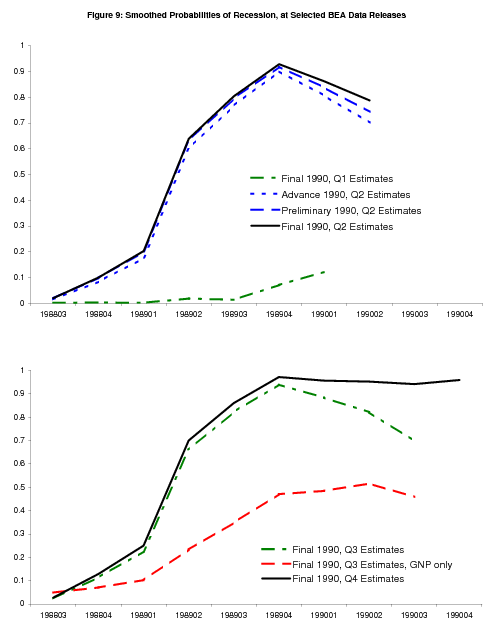
Figure 9 shows smoothed probabilities around the start of the 1990-91 recession, and illustrates how critical the information provided in BEA's annual revisions can be. The economy seems to be sailing along smoothly until the annual revision that comes with the 1990Q2 data: the four quarterly GNP growth rates in 1989 (in chronological order) are revised down from 3.7%, 2.5%, 3.0% and 1.1% to 3.6%, 1.6%, 1.7% and 0.3%, an average downward revision of about three quarters of a percentage point. The quarterly growth rates of GNI are revised down even more, from 4.3%, 2.0%, 3.5% and 1.4% to 3.4%, 0.9%, 1.4% and -0.7%, an average downward revision of about one and a half percentage points. With the revisions, the probabilities from the model indicate quite clearly that economy was in recession or its low-growth phase in the second half of 1989 (see the dotted blue, dashed blue, and solid black lines in the top panel).¹² Positive growth from 1990Q1 to 1990Q3 brings down the probabilities in those quarters, but the growth rates are low enough to keep the probabilities well above 50%. Negative growth in 1990Q4 solidifies the view that the economy is in recession (see the solid black line in the bottom panel).

The red dashed line in the second panel of Figure 9 shows smoothed probabilities from the univariate model with GNP alone, after the "final" 1990Q3 data release. The comparatively large downward revisions to GNI growth do make a critical difference, especially the 2.1 percentage point downward revision that takes 1989Q4 GNI growth down to -0.7%. With GNP growth alone, the probabilities drift up but never cross the 50% threshold before the release of 1990Q4 data; these probabilities paint a much more ambiguous picture of the economy.

The importance of the revisions provides a means for reconciling the results in this paper, showing that GDI provides value over GDP in identifying recession in real time, with the results in Nalewaik (2006). That paper analyzes the properties of constructed time series of GDP and GDI where each quarterly observation is the "final" current quarterly growth rate released in real time three months after that quarter closed. It shows that the larger mean spread and lower conditional variance of GDI relative to GDP are less evident in these early-vintage "final" current quarterly growth rates - i.e. the statistical advantages of GDI in identifying recessions appear much more clearly in data that have passed through annual revisions. A reader may wonder how it is possible to find the real time results that we have found so far given that fact.

To square these facts, return to the point made in the discussion of two-stage updating: prior probabilities have an important impact on current probabilities through the Markov transition matrix. The prior probabilities, computed from data that have passed through annual revisions, are more accurate in the bivariate model than in the univariate GDP model, and these more accurate prior probabilities translate into more accurate current probabilities through the time dependence in the model. This holds true even if the latest current quarterly estimate of GDI is not necessarily any more accurate than the latest current quarterly estimate of GDP. The influence of the annual revision to the 1989 data on the 1990 probabilities of recession shows how this can work.

The 2001 recession (beginning)

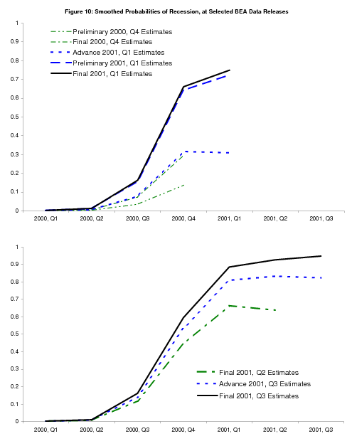
Figure 10 shows smoothed probabilities around the start of the 2001 recession. In 2000Q4, "advance" GDP growth (smoothed probabilities not shown) comes in at 1.4%, and is revised down to 1.1% in the "preliminary" release, which leads to an uptick in the probability of recession to about 10%. The first GDI estimate for this quarter arrives with BEA's "final" release, and its growth of 0.3% (with GDP growth of 1.0%) bumps up the probability of recession to about 30%. In 2001Q1, when the NBER dates the start of the recession, "advance" GDP growth starts at 2.0%, again giving a probability of recession of about 30%, but when GDI growth comes in at 0.1% with the "preliminary" release, the probability of recession immediately jumps above 50%. The "final" values for 2001Q1 have GDP and GDI growth running at 1.2% and 0.0%, respectively. This case is somewhat different than the 1990 recession just discussed: it is the latest values of GDI that provide the critical information, rather than revised estimates from prior years.

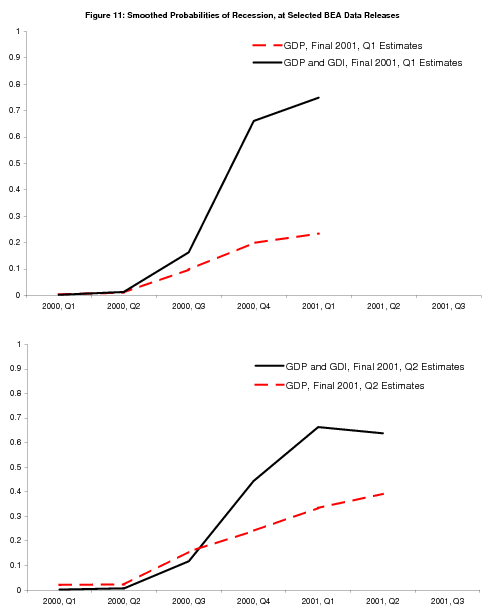
The "final" values for 2001Q2 have GDP and GDI growth at 0.3% and 1.2%, respectively; the stronger value for GDI leads to a slight downtick in the probability of recession, but the probability remains above 50%. Figure 11 compares bivariate probabilities of recession computed in 2001Q1 and 2001Q2 with the corresponding univariate GDP probabilities. The differences are striking: the probabilities of recession computed using GDP alone are much lower than those using GDP and GDI. Negative values for GDP and GDI growth in 2001Q3 (not shown) solidify the view that the economy is in recession in both models, but these data were released by BEA after other events had made the recession abundantly clear. It was only the bivariate model that sounded clear warning bells months earlier.

The 2001 recession (end)

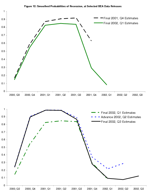
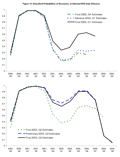
Before analyzing further the superior performance of GDI in recognizing the start of the 2001 recession, Figures 12 and 13 show the evolution of the ending point of the 2001 recession with the arrival of new data. "Final" GDP and GDI for the 2001Q4 registered at 1.7 and 3.1%, bringing down the probability of recession somewhat, and very strong 2002Q1 growth rates of 6.1% and 5.4% bring the probability of recession below 50%, as shown in the green line in the top panel of Figure 12. The 2002Q2 "advance" release came with an annual revision that was quite informative. The 2001 growth rates of GDP and GDI were both revised down, making the recession clearer in the data, and the 2000Q4 growth rate of GDI was revised down to -0.5% as well, which is reflected in the smoothed probabilities which now assign high probability to the recession starting in this quarter. The 2002Q1 growth rates of GDP and GDI were also revised down, GDP from 6.1% to 5.0%; this particular quarterly growth rate was ultimately revised down further to 2.7%.

The 2002 annual revision marked the beginning of a new practice for BEA regarding the GDI growth rates: initially at the time of the "final" current quarterly release, and later accelerated to the "preliminary," BEA began revising employee compensation and GDI for the prior quarter, replacing the current quarterly estimates of wages and salaries based on Current Employment Statistics (CES) survey data with estimates based on what is often called the ES-202 data. The ES-202 data are superior to the CES data for at least two reasons: (1) the CES data are computed from samples of businesses, while the UI data are computed from the entire universe of businesses from which the CES survey is drawn, and (2) the UI data include bonuses, gains from exercising nonqualified stock options and other irregular forms of pay not captured by the CES survey. Prior to this change the ES-202 data had been incorporated at annual revisions; the new practice allows BEA to produce more accurate GDI estimates sooner.

Figure 13 is where we begin to see the impact of the ES-202 revisions. We have, with the "final" 2002Q4 release, a downward revision to 2002Q3 GDI growth from 2.2% to 0.8.¹³ 2002Q4 GDP and GDI growth are weak as well ("final" values at 1.4% and 2.4%), and we begin to see the probability of recession creeping back upwards. "Final" 2003Q1 GDP and GDI growth are 1.4% and 1.9% with 2002Q4 GDI revised down to 1.2%,¹⁴ and the probability of recession has crept back up above 50% at this point. 2003Q1 GDI growth is revised down with the 2003Q2 release, but "final" 2003Q2 GDP and GDI both come in stronger, at 3.3% and 3.1%, and the 2003Q3 estimates clearly demarcate the end of the recession with 8.2% GDP and 5.8% GDI growth rates. With the "preliminary" 2003Q3 release came a benchmark revision that confirmed the downward ES-202 revisions at the end of 2002, increasing their size to the point where the smoothed probabilities suggest the recession of 2001 did not actually end until 2003Q2, as can be seen clearly in Figure 7.

The 2001 recession (beginning), reprise

It is natural to ask whether any particular component of GDI plays an outsized role in its superiority in recognizing the start of recessions. For the 2001 recession, a clear candidate emerges: corporate profits. The table below shows the prevailing estimates of corporate profits for selected "final" current quarterly data releases around the start of the recession, the results of the 2001 annual revision that came with the 2001 second quarter numbers, and the latest estimates of corporate profits for that time period:

Corporate Profits

	"final" curr. qtr.	2001 annual revision	latest (2005Q3)
1999Q4	919.4	857.6	869.3
2000Q1	965.6	870.3	832.6
2000Q2	963.6	892.8	833.0
2000Q3	970.3	895.0	811.8
2000Q4	914.7	847.6	794.3
2001Q1	869.0	789.8	778.7
2001Q2	759.8	759.8	783.1
2001Q3	697.0		714.5

Real GDI growth rates of around zero in 2000Q4 and 2001Q1 pushed the estimated probability of recession from the bivariate model above 50% in 2001Q1, and the table shows that corporate profits fell sharply in these quarters. If corporate profits had been just flat rather than showing steep declines, real GDI growth in 2000Q4 and 2001Q1 would have come in around 3 percent and 2 percent, respectively.

It is notable that most of the fall in corporate profits in 2000Q4 and 2001Q1 was subsequently revised away by BEA, as part of it was simply a correction of estimates that were too high at the end of the expansion. Much of the decline in corporate profits now appears to have occured earlier, in 2000Q1 and 2000Q3.¹⁵ Was it simply fortuitous measurement errors that drove GDI's success in identifying the start of the 2001 recession? Perhaps, and that would argue for caution in relying too much on GDI to identify recessions going forward. Another reason for caution is the results in Nalewaik (2006) showing that the statistical advantages of GDI over GDP are not as evident in the "final" current quarterly estimates as in estimates that have passed through annual revisions. This result is not inconsistent with the real time analysis here; as the discussion of the 1990 recession makes clear, more accurate prior probabilities of recession, based on data that have passed through annual revisions, typically lead to more accurate current probabilities of recession. However these results do suggest that it would be imprudent to rely on GDI exclusively; careful examination of the information in both GDP and GDI should produce the best results going forward.

The corporate profits mismeasurement issue is certainly important, but measurement errors in other components of GDI are important to considered as well. In particular, note that around the start of the latest recession in 2000Q4 and 2001Q1, the changes in "final" current quarterly employee compensation were subsequently revised down by about 65 billion in total, approximately offsetting the upward revisions to the change in corporate profits. The more timely incorporation of ES-202 data discussed earlier may reduce these measurement errors going forward, possibly improving the ability of current quarterly GDI to identify the start of recessions.¹⁶In a related point, the incorporation of ES-202 information likely moves the statistical properties of a GDI estimate closer to the statistical properties of an estimate that has passed through annual revisions. Only the last one or two time series observation would typically exhibit the statistical properties of the "final" current quarterly estimates under the new procedure, compared to the last two to five observations under the old procedure depending on when the last annual revision occured. So the new procedure may diminish somewhat the relevance of the results in Nalewaik (2006) on the "final" current quarterly estimates.¹⁷

5 Robustness Check: Accounting for the Mid-1980s Reduction in Variance of GDP and GDI Growth

A large number of papers have documented and analyzed the now-evident reduction in variance of the growth rate of the economy that occurred sometime in the mid-1980s - see McConnell and Perez-Quiros (2000). When Fixler and Nalewaik (2004) allow for a break in the variance of GDP and GDI in 1984Q3,¹⁸ they find that the variance of GDI growth exceeds that of GDP growth both before and after the break, whereas without the break, the reverse is true. While those results derive from a different sample period than that considered here, and unconditional variances are not quite the same as conditional variances from a Markov switching model, given our finding that the lower conditional variance of GDI drives its dominance of GDP in the bivariate model, it is important to check whether this result holds when we allow for the break in variances.

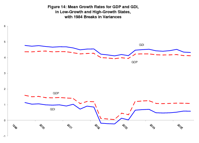
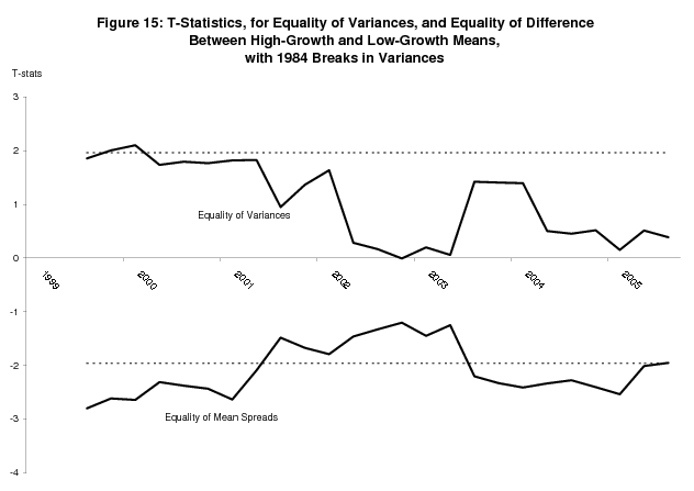
Table 5 shows estimates of the bivariate model with a 1984Q3 break in the variance parameters, estimated using data from the 2005Q3 "final" current quarterly release. As before, these parameters are estimated via the EM algorithm, which required some straightforward modifications to the formulas in (5). In addition to the massive decreases in variance that we see after the break, the variance of GDI relative to the variance of GDP increases, although the variance of GDP remains larger, unlike the unconditional estimates of Fixler and Nalewaik (2004). The mean growth rates of GDP and GDI in expansions decrease, the mean growth rates of GDP and GDI in recessions increase,¹⁹ and the mean spread for GDI increases relative to the mean spread for GDP. We estimated this model for every "final" current quarterly release since 1999Q3, around the time when academic papers on the reduction in variance began to appear, and Figure 14 plots the mean spreads for each one of these estimates. We see the consistently larger mean spread for GDI. Figure 15 shows t-statistics for the equality of the (post-break) variances, and for the equality of the mean spreads. Interestingly, while the difference between the variances quickly loses its statistical significance, the difference between the mean spreads is now statistically significant at the 95% significance level for many sets of estimates. This argues that the advantage of GDI over GDP in identifying recessions is robust to the inclusion of the variance breaks; however the basis for the advantage of GDI shifts to a greater mean spread from a smaller conditional variance.

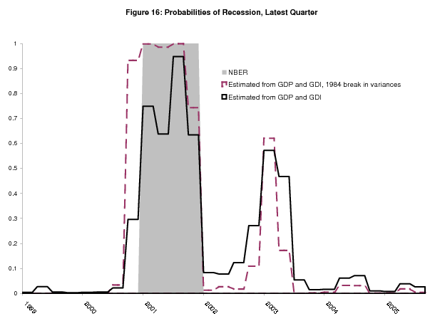
Figure 16 plots the probability of recession for the latest quarter from each of these 1999Q3 to 2005Q3 real time estimates of the model, along with the familiar estimates without the break. Given the tiny post-break conditional variances, the model confidently calls the start of the recession in 2000Q4. Although subsequent evidence confirmed this result, concerns about over-fitting argue that this model should be used with caution.

6 Conclusions

This paper estimates Markov switching models for GDP and GDI in real time, showing that GDI has recognized the start of recent recessions faster than GDP. Some combination of the following two statistical facts accounts for this: (1) the deceleration of GDI growth in recessions is greater than the deceleration of GDP growth, (2) the variance of GDI conditional on the estimated state of the world is lower, so it provides a more accurate signal of the state. In the baseline specification, the lower conditional variance is the key factor, although the greater deceleration becomes more important after accounting for the mid-1980s moderation in the variance of the growth rate of the economy. While the paper points out some caveats regarding the measurement of GDI, overall the results suggest that in analyzing the current state of the economy, GDI should be scrutinized closely along with GDP. The bivariate Markov switching model employed in this paper is a useful tool for summarizing the information in both estimates about the state of the economy.

Going forward, there is some reason to believe that BEA's real time estimates of employee compensation for current quarters will be better than they have been in the past. First, BEA now incorporates what are essentially census counts of firms' wages and salaries paid, from the BLS's ES-202 program, into its quarterly estimates with a shorter lag than it has in the past, about 5 months after the quarter closes.²⁰ Second, the extrapolators BEA uses before it has access to the ES-202 are likely to improve as well, as BLS rolls out more comprehensive earnings measures over the next couple of years as part of its monthly Current Employment Statistics (CES) data releases. Since employee compensation makes up the bulk of GDI, these changes give further reason to study GDI carefully in analyzing the current state of the economy in the years to come.

An interesting side result of the paper is that, over the past 25 years, the Markov switching models have gradually increased the mean growth rates of GDP and GDI in low-growth periods, to the point where they are now around zero rather than significantly negative. Going hand in hand with this, these low-growth periods as defined by the switching models are now substantially longer than recessions as defined by the NBER's peak and trough dates.

Appendix A: Derivation of the Smoothing Algorithm
For Partially Updated Probabilities in Last Sample Period

The proof that Kim's (1994) smoothing algorithm works when the last observation in the sample is only partially updated, as in (6), requires only very minor modifications to the proof provided in Appendix 22.A of Hamilton (1994); what follows below draws heavily from that Appendix.

The probability of recession in the last period of the sample, updated with respect to the partially available information, is . We'll start by considering how to produce the smoothed probability of recession one period earlier, or . The first step is to show that , moving to more general notation of arbitrary states and periods. We have:

where is the joint density-distribution function of and , as Hamilton (1994) puts it. A key assumption of the model is that, for the joint density:

so the joint distribution of the variables, conditional on the current state, is independent of prior states. We assume this is true for the marginal density of as well, so:

in which case the in A.1 cancel, which proves the first step. Next, consider:

where the last line is proven in Hamilton (1994). Then:

The smoothing algorithm of Kim (1994) produces this result; the only difference is that replaces the standard .

Next consider the smoothed probabilities for a period arbitrarily far back in time. Using the same arguments as in Hamilton (1994), one can prove that:

Then as in A.2, we can show:

and parallelling A.3, we have:

This justifies use of the Kim (1994) algorithm arbitrarily far back in time.

Bibliography

Andrews, Donald W.K. "Tests for Parameter Instability and Structural Change with Unknown Change Point"

Econometrica, 1993

(61), pp. 821-856.

Chauvet, Marcelle. "An Econometric Characerization of Business Cycle Dynamics with Factor Structure and Regime Switching"

International Economic Review, 1998

(39), pp. 969-996.

Chauvet, Marcelle and Hamilton, James. "Dating Business Cycle Turning Points"

in Nonlinear Analysis of Business Cycles, edited by Costas Milas, Philip Rothman, and Dick van Dijk, Elsevier, forthcoming.

Chauvet, Marcelle and Piger, Jeremy. "Identifying Business Cycle Turning Points in Real Time",

Federal Reserve Bank of Atlanta working paper 2002-27, 2002.

Economic Report of the President, 2004

Fixler, Dennis J. and Nalewaik, Jeremy J. "News, Noise, and Estimates of the True Unobserved State of the Economy",

BEA working paper 2004-08, 2004.

Friedman, Milton. "The 'Plucking Model' of Business Fluctuations Revisited"

Economic Inquiry, 1993 pp. 171-177.

Grimm, Bruce T. "Alternative Measures of U.S. Economic Activity in Business Cycles and Dating",

BEA working paper 2005-05, 2005.

Hamilton, James D. "A New Approach to the Economic Analysis of Nonstationary Time Series and the Business Cycle"

Econometrica, 1989

(57), pp. 357-84.

Hamilton, James D. "Analysis of Time Series Subject to Changes in Regime"

Journal of Econometrics, 1990

(45), pp. 39-70.

Hamilton, James D. Time Series Analysis.

Princeton, Princeton University Press (1994).

Kim, Chang-Jin. "Dynamic Linear Models with Markov Switching"

Journal of Econometrics, 1994

(60), pp. 1-22.

Kim, Chang-Jin and Nelson, Charles R. "Friedman's Plucking Model of Business Fluctuations: Tests and Estimates of Permanent and Transitory Components"

Journal of Money, Credit and Banking, 1999 (31), pp. 317-334.

McConnell, Margaret M., and Perez-Quiros, Gabriel. "Output Fluctuations in the United States: What Has Changed Since the Early 1980s?"

American Economic Review, 2000 (90), pp. 1464-1476.

Nalewaik, Jeremy J. "Towards More Accurate and Timely Estimated Probabilities of Recession: Incorporating Vintage Differences and Forecasts into Markov Switching Models."

Manuscript, 2006

Seskin, Eugene P., and McCulla, Stephanie H. "Annual Revision of the National Income and Product Accounts,"

Survey of Current Business, August 2002, pp. 7-34.

Sichel, Dan. "Inventories and the Three Phases of the Business Cycle"

Journal of Business and Economic Statistics, 1994 (12), pp. 269-77.

Table 1:
Real Time Estimates of Markov Switching Model for GDP

Data as of 1978Q1 Final Curr. Qtrly. Release

Estimate	5.05	-1.59	7.71	0.94	0.79	1.00
(s.e.)	(0.41)	(0.91)	(1.37)	(0.04)	(0.11)	(1.03)

Data as of 2005Q3 Final Curr. Qtrly. Release

Estimate	4.51	-0.22	8.37	0.93	0.79	1.00
(s.e.)	(0.32)	(0.85)	(1.03)	(0.03)	(0.08)	(2.91)

Table 2:
Real Time Estimates of Markov Switching Model for GDI

Data as of 1978Q1 Final Curr. Qtrly. Release

Estimate	5.09	-1.71	6.84	0.94	0.80	1.00
(s.e.)	(0.38)	(0.80)	(1.19)	(0.03)	(0.11)	(1.13)

Data as of 2005Q3 Final Curr. Qtrly. Release

Estimate	4.71	-0.22	6.40	0.94	0.82	1.00
(s.e.)	(0.25)	(0.53)	(0.74)	(0.02)	(0.07)	(1.17)

Table 3:
Real Time Estimates of Bivariate Markov Switching Model for GDP and GDI

Data as of 1978Q1 Final Curr. Qtrly. Release

Estimate	5.05	5.09	-1.59	-1.71	7.72	6.85	6.86	0.94	0.80	1.00
(s.e.)	(0.40)	(0.38)	(0.82)	(0.79)	(1.35)	(1.20)	(1.24)	(0.03)	(0.11)	(1.22)

Data as of 2005Q3 Final Curr. Qtrly. Release

Estimate	4.60	4.71	0.13	-0.22	8.48	6.40	5.85	0.93	0.82	1.00
(s.e.)	(0.28)	(0.25)	(0.55)	(0.53)	(0.94)	(0.73)	(0.75)	(0.03)	(0.07)	(1.17)

Table 4:
GDI Parameters
Evaluated Using Smoothed Probabilities from Univariate GDP Model

Data as of 1978Q1 Final Curr. Qtrly. Release

Estimate	5.07	-1.64	7.02
(s.e.)	(0.41)	(0.99)	(1.29)

Data as of 2005Q3 Final Curr. Qtrly. Release

Estimate	4.47	-0.12	7.37
(s.e.)	(0.28)	(0.91)	(0.86)

Table 5:
Real Time Estimates of Markov Switching Model for GDP and GDI,
1984Q3 Breaks in Variance Parameters
Data as of 2005Q3 Final Curr. Qtrly. Release

Estimate	4.12	4.32	1.08	0.58	15.18	11.46	11.54
(s.e.)	(0.23)	(0.22)	(0.39)	(0.41)	(2.42)	(2.06)	(2.11)

Estimate	2.62	2.40	1.16	0.93	0.81	1.00
(s.e.)	(0.40)	(0.44)	(0.38)	(0.03)	(0.07)	(1.60)

Footnotes

* Comments Welcome. Board of Governors of the Federal Reserve System (e-mail: [email protected]). The views expressed in this paper are soley those of the author. Much of this work was completed while the author was a research economist at the U.S. Bureau of Economic Analysis (BEA). I thank Doug Elmendorf, Charles Fleischman, Bruce Grimm, David Lebow, Jeremy Rudd, Dan Sichel, John Stevens and seminar participants at BEA and the Board of Governors for comments. Return to Text

1. One advantage of the models based on monthly indicators, compared to models based on quarterly NIPA aggregates such as GDP, is timeliness. Nalewaik (2006) shows how to incorporate forecasts of GDP (and GDI) from monthly or weekly indicators into the Markov switching models discussed here. Those models retaining the comprehensiveness of GDP while exploiting the added timeliness of the monthly data. Return to Text

2. The BEA may emphasize GDP because GDP is produced in a more timely manner than GDI, a fact whose implications are discussed later in the paper. The BEA may also emphasize GDP because they produce price deflators for the detailed components of GDP but not GDI. Return to Text

3. These smoothed probabilities, also called two-sided probabilities, use time series realizations of GDP and GDI from the future as well as the past to estimate the probability of recession at any given date, and hence are more accurate than the one-sided probabilities using only past realizations available in real time. Return to Text

4. GNP rather than GDP was BEA's featured aggregate until 1991Q3 when GDP took over. The difference between GDP and GNP, net factor payments, is usually pretty small, typically not altering the annualized quarterly growth rates of the time series by more than a couple tenths of a percentage point. Return to Text

5. While deflating nominal GDI by the GDP deflator to estimate real GDI is not entirely satisfactory, a better procedure did not immediately present itself. Return to Text

6. While the two state model is most popular in the literature, a three state "plucking" model, with GDP bouncing back rapidly after a recession, has been examined quite a bit as well: see Friedman (1993), Sichel (1994), and Kim and Nelson (1999). The last two recessions, exhibiting periods of slow growth after the NBER-defined end date, argue against the use of the three state model in analyzing recent history. Return to Text

7. Chauvet and Hamilton (2005) provide some non-parametric evidence of normality in a regime-switching context, using the NBER's start and end dates for recesssions. Return to Text

8. As noted earlier, the "final" release for quarter occurs close to the end of quarter . A significant amount of data on quarter has been released at this point, which could potentially be exploited to produce more timely estimated probabilities of recession - this is examined in Nalewaik (2006). Return to Text

9. We shade areas in a somewhat expansive way; the NBER dates the beginning and end of recessions by month; if any month of a quarter is classified by the NBER as in recession, we shade the entire quarter. For example, the NBER says the last recession in the plots started in March 2001 and ended in November 2001; we shade both 2001Q1 and 2001Q4. Return to Text

10. Fixing the data and comparing the probabilities of recession computed using the different set of parameter estimates can give a sense of the impact of these parameter changes. Examining the 1960 recession using 1978Q1 vintage data, real GNP growth rates of -0.97%, -1.72%, -2.05% in the last three quarters of 1960 translate into one-sided probabilities of recession of 41%, 92%, and 99% using 1978Q1 parameters, and probabilities of 29%, 77%, and 95% with 2005Q3 parameters. These differences are not large, but with 2005Q3 parameters, the signals are a bit more muddled. Return to Text

11. The large jumps here in 1985, 1991, and 1995 correspond to benchmark revisions to the NIPAs. There were also benchmark revisions in 1980, 1999, and 2003. Return to Text

12. We can see now that figure 3 is somewhat misleading for the start of this recession; the bump above 50% we see in 1990Q2 in that figure comes with large increases in probabilities of recession for prior quarters, which would surely have been of interest to analysts of the state of the economy at the time. Return to Text

13. After BEA's 2005 annual revision, this growth rate stood at -0.4%. Return to Text

14. After BEA's 2005 annual revision, this growth rate stood at currently stands at 0.3%. Return to Text

15. The overall decline in corporate profits from 1999Q4 to 2001Q3 is about 150 billion in the 2005Q3 vintage data, still substantial. Return to Text

16. Seskin and McCulla (2002), in their description of BEA's annual revision for that year, explicitly point to the incorporation of ES-202 data as the reason for the downward revision to employee compensation in 2001. Return to Text

17. The earlier incorporation of the ES-202 data may not be an unambiguous improvement, however. For example, these data pick up gains from exercising nonqualified stock options, which typically require offsetting reductions to corporate profits; if BEA does not accurately capture these offsetting reductions for its first few corporate profits estimates, because it must rely on incomplete surveys and publicly available corporate financial statements, then additional measurement error could be introduced into GDI. The extent to which this will prove to be a problem with the new procedures is unclear. Return to Text

18. Fixler and Nalewaik (2004) conduct likelihood-ratio break point tests, following Andrews (1993), to arrive at this break point. Return to Text

19. Concerns about overfitting stopped us from modelling breaks in these parameters as well as the variance parameters. Return to Text

20. The earlier incorporation of the ES-202 data does have the potential to introduce some problems; see footnote 17. Return to Text

^♣ This version is optimized for use by screen readers. Descriptions for all mathematical expressions are provided in LaTex format. A printable pdf version is available. Return to Text

Home | Economic Research and Data
Accessibility | Contact us
Last update: May 10, 2007