
A Cohort-Based Model of Labor Force Participation
Keywords: Labor force, aging, labor supply, labor force participation
Abstract:
The probability that an individual participates in the labor force declines precipitously beyond age 50. This feature of labor supply suggests that ongoing shifts in the age distribution of the population will put substantial downward pressure on the aggregate labor force participation rate. However, the aggregate rate is also influenced by trends within age groups. Neglecting to model both within-group influences and shifting population shares will doom any estimate of aggregate labor supply. We develop a model that identifies birth cohorts' propensities to participate, uses these propensities to derive age-specific trends in participation rates, and explicitly incorporates the influence of shifting population shares in estimating aggregate labor force participation.
I. Introduction
Growth in labor productivity and growth in labor input determine output growth. In recent years, technological developments have changed how many economists think about growth in labor productivity. However, in the coming years, the aging of the population will change how economists think about the growth in labor input in the United States. In only the last few years, as the oldest baby boomers turned 50, then 55, and then 60, an almost unremarked economic change slowly surfaced: They became less likely to participate in the labor force. Obscured by a labor market slump, the aging of the population began to put downward pressure on aggregate labor supply, marking the start of what is likely to be a sharp deceleration in labor input that will last another half-century.
This structural change represents the type of economic turning point typically missed by backward-looking time series models. In this paper we propose an empirical model that explicitly incorporates the ongoing demographic changes and offers an alternative to commonly used filters and time series models for projections and trend-cycle decompositions.1 The model we propose captures well the historical changes in labor force participation and addresses a variety of substantive economic questions about aggregate labor supply.
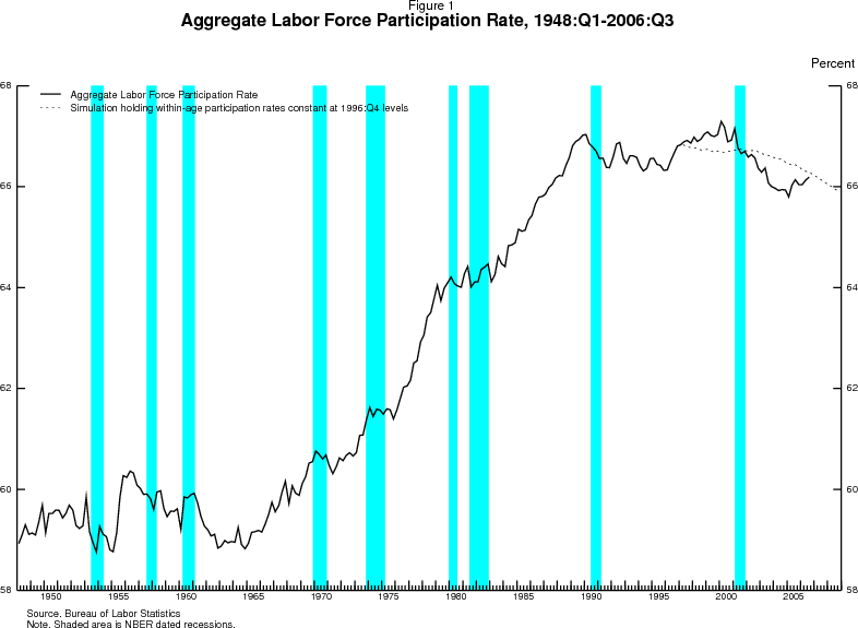
The solid line in figure 1 shows the aggregate labor force participation rate in the United States from 1948 onward. Broadly speaking, this rate can be described as having had three regimes: a period of relative stability until the mid-1960s, a period of steady increase between the mid-1960s and the late 1980s, and a recent period in which those increases have ended. This experience was dominated by movements in women's labor force participation, which rose sharply over the 25 years following 1965, and leveled off after about 1990.
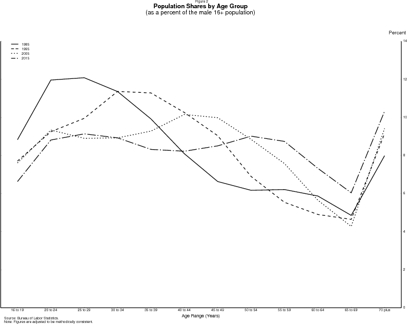
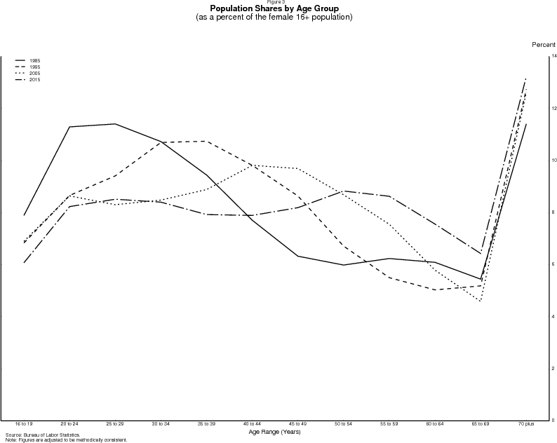
However, the dominant development in coming years will likely be the evolution of the age distribution of the population. As shown in figure 2 for men and figure 3 for women, as the baby-boomers have aged and life expectancies have increased, the population share of older Americans has begun to rise. Since 1995 the population bulge comprising people in their 30s has moved on to older ages--ages with lower participation rates. Barring a major change in the participation behavior of older persons, the shift of the population distribution away from prime-working ages will put significant downward pressure on the nation's labor force participation rate.
To put the potential magnitude of this demographic shift into perspective, the dashed line in figure 1 shows a simulated path for the aggregate labor force participation rate that holds constant the participation rates of individual age groups at their 1996 levels but allows population shares to evolve as projected by the Census Bureau. The shift in population shares alone is already putting downward pressure on the participation rate. Although not shown, the shift in population shares would, ceteris paribus, lower the participation rate from about 66 percent in 2005 to about 64 percent by 2015, and push it below 60 percent by 2030. Thus, absent other changes, the aging of the population has the potential to undo the increases in participation brought about earlier by the increased entry of women into the labor force.
As these changes in the age distribution unfold, it is unclear how the within-group trends will adapt to offset--or perhaps evolve to exacerbate--the declines induced by aging. (Indeed, thus far it appears that within-group trends have mostly exacerbated the decline.) Our aim in this paper is to present a model that decomposes the movements in labor force participation into components driven directly by the aging of the population and by trends within age groups, as well as the business cycle.2
The paper proceeds as follows: The next section describes the shifts underway in the nation's age distribution and decomposes the influence of each age group's changing population share on the aggregate participation rate. The third section discusses the influence of birth cohort. The fourth section outlines a non-parametric model of aggregate participation that identifies birth cohorts' propensities to participate and a baseline age profile, and explicitly incorporates the changing population shares. The fifth section discusses several complications that arise in estimation, and the sixth section discusses the basic model results. Sections seven and eight extend the model to allow the age profiles to evolve over time along with other types of structural change in the labor market, and discuss the results. The ninth section focuses on the past several years, and the tenth section concludes.
II. The influence of population shifts
In any period, the low-frequency changes in the aggregate participation rate can be decomposed into the influence of changes in the demographic distribution of the population and the influence of changes in labor supply behavior within the various demographic groups. One useful decomposition of
the aggregate labor force participation rate into the contributions of the participation rates and population shares of the several groups follows the identity,
Changes over time in the first term can be interpreted as the contribution of changes in a group's population share to the evolution of the overall participation rate, and changes over time in the second term can be interpreted as the contributions of changes in the group's participation rate to that evolution.3
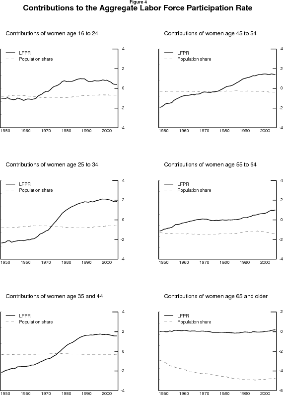
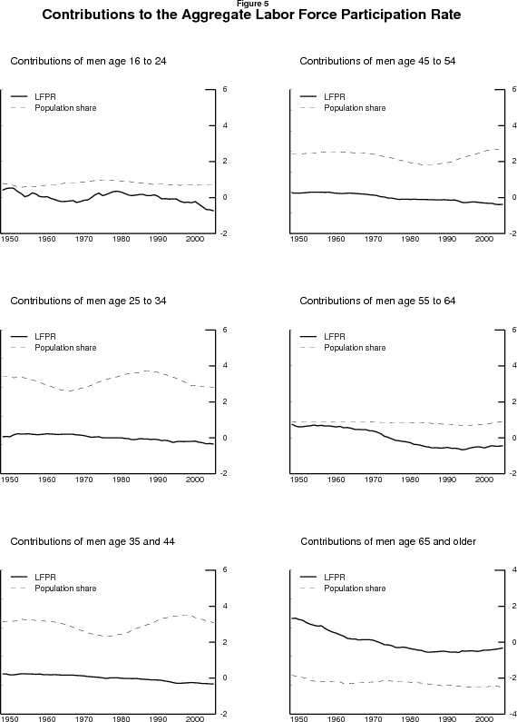
Figures 4 and 5 illustrate this decomposition for twelve age-sex groups. Looking back over history, the evolution of participation rates for particular groups has been the more important factor, although demographic shifts have played a role as well. Over the period roughly from 1948 to 1965, the aggregate participation rate was fairly flat, as an increase in the share of the population (especially women) over age 64 and declines in the participation rates of men in several age groups were offset by an increase in the participation rates of prime-aged (25-64) women. Over the period roughly from 1965 to 1990, the big story was a large increase in the participation rates of young and prime-aged women, which overwhelmed decreases in the participation rates of prime-aged and older men, and a further increase in the share of the population (again especially women) over age 64. From roughly 1990 to 2000, further, smaller, increases in the participation rates of prime-aged women were offset by small declines in the participation rates of young and prime-aged men. Since then, beginning at about the same time as the 2001 recession, the aggregate participation rate has fallen. How much of this is best described in terms of these sorts of low-frequency movements, and how much in terms of the business cycle and other temporary phenomena, is a question we will return to below.
III. The influence of birth-year cohort
The increases in the participation rate of women, and the concomitant decline in the participation rate of men, likely reflected numerous factors such as evolving tastes, reproductive technology, wealth, education, social attitudes, and the development of the retirement, welfare, and financial systems. Some of these changes arguably were to be internalized into the behavior of new generations more easily than into the behavior of mature cohorts who had already made "sticky" choices. And, indeed, among women in particular, much of the change in the aggregate participation rate appears to have resulted from progressively higher average participation rates of successive cohorts, as opposed to increases in age-adjusted participation within cohort; that is, entering cohorts of women had higher participation rates for their ages than did the cohorts who proceeded them.
The model we propose in the next section estimates observed attachment of cohorts in the labor force as a basis for considering their future attachment, building on a rich literature. John D. Durand (1948) recognized policymakers' need for labor force and participation rate projections for the post-war period. Not surprisingly, his work modeled demographic shifts and trends toward early retirement. However, he explicitly recognized an intrinsic propensity to supply labor that was birth-year specific: "As they grew older, each successive generation of women seems to have retained the greater propensity to be in the labor force which it developed in early adulthood, and so the higher percentages of labor force members have gradually been transmitted throughout the age groups from the late 20's to the early 60's," he wrote, relying on decennial censuses from 1890 to 1940 for his analysis.4
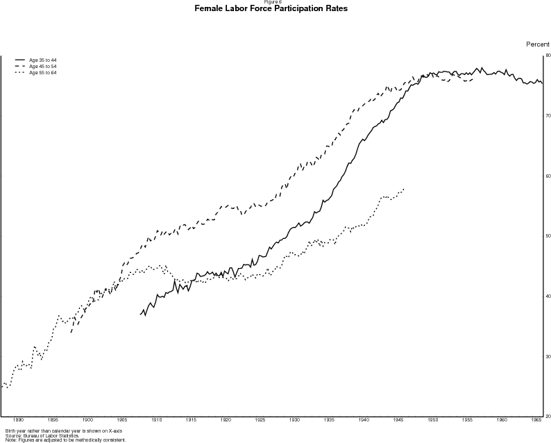
Durand's observation was prescient. Figure 6 shows the labor force participation rates for three age groups of women: age 35 to 44, age 45 to 54 and age 55 to 64. Each line shows the participation rate of an age group over time. However, instead of the year of observation, the x-axis shows the birth year for the middle age of the group. In this way, the lines are shifted so that each birth cohort is vertically aligned with itself at different ages. The participation rate of the 45-54 year old group (the dashed line) appears to exhibit three rough inflections, in the vicinity of years 1960, 1975, and 1997, corresponding to the cohorts born around 1910, 1925, and 1947. The first two of these inflections line up well with the 55 to 64 year old group (the dotted line), meaning that the inflection points in the two age groups seem to be related to when the cohorts born in 1910 and 1925 passed through. The cohort associated with the third inflection (those born around 1947) are not quite old enough to exhibit that inflection in the older group. But that third inflection point can be seen when that cohort was 35-44 years old (the solid line). Similarly (not shown), beginning in the mid-1960s and ending in the late 1970s, successive cohorts of 16-24 year old women had higher participation rates than their predecessors. Participation rates of successive cohorts 25-34 year olds stopped rising about ten years later, in the late 1980s, suggesting that the participation rate in each of these age groups at a given time is at least partly related to which birth cohort is passing through that age at that time.
These coincidences suggest that birth cohort plays a significant role in determining the pattern in participation of an age group over time. Of course, not all age groups line up so well by birth year, or at least not all of the inflection points line up. Clearly, there have been developments in participation that are not well-represented by the aging of birth cohorts, and may, for example, be better represented as changes in the shape of the age profile. We will return to these factors below. Nevertheless, the apparent importance of differences in the participation rates of successive cohorts means that the evolution of the aggregate participation rate ought to be at least partly predictable. That is, the difference between the participation behavior of a given birth cohort at a younger age and that of earlier cohorts at that same younger age tells us something about the difference between the participation behavior of that birth cohort at an older age and of those earlier cohorts at that same older age. For example, the fact that at age 35 women born in 1945 had higher participation rates than did women born in 1935 could have led us to predict that at age 50 the women born in 1945 would also have higher participation rates than did the women born in 1935.
Thus, an empirical model should incorporate the already observed behavior of birth cohorts as they have passed through each age group and use that information to project how that intrinsic attachment will influence the participation rates of older age groups in the future. However, in addition to cohort effects, the model should also incorporate the influence of age, and contemporaneous influences--leading to the well-established identification problem of separately identifying these three linearly dependent determinants of participation: age, cohort and year. In fact, the model proposed in the next section is similar to that of Greenberg, et. al. (1950) who decomposed the incidence of syphilis into age, birth year, and contemporaneous time effects. Because the three dimensions are linearly dependent, the authors utilized functional form assumptions to separately identify the three influences. We extend the earlier authors' time series application to a panel framework. We consider a similar problem in the context of labor force participation, and explore variation in age and cohort profiles that builds on the earlier statistical research. The resulting framework provides economically meaningful estimates of the role of age, birth cohort, and year in labor force participation rates.
IV. The Basic Model
In the previous two sections we have argued for the importance of two regularities in explaining changes in the labor force participation rate: changes in the propensity to participate as a person ages, and differences in propensities to participate across birth cohorts. In this section we develop a model that attempts to identify the influence of various factors that can be represented on average by a person's birth cohort, those that can be represented on average by a person's age, and those that can be represented by the state of the business cycle. The model is an attempt to use the observed history of each cohort's labor force attachment to inform us about its present and future attachment, and to combine our knowledge of cohort behavior with known demographic changes into a coherent framework. Later, we enhance the model to incorporate measurable trends in human capital, family structure, and retirement financing. But first we are interested to see how far age and cohort alone can go in explaining the history of the labor force participation rate.
Because both the average participation rates and the age profiles of participation have historically been so different for men and women we model participation separately by gender. We assume that the labor force participation rate of men or of women of a particular age ![]() in year
in year ![]() can be specified as
can be specified as
where LFPR is the participation rate;
This specification assumes that each birth-year cohort has a general propensity to participate in the labor force that is determined by various unmeasured factors. This propensity is quantified by ![]() , the log of which can be viewed as a cohort-specific intercept. However, the members of different cohorts share a common baseline pattern of participation over the life cycle, being, for example, low when at school or retirement ages and higher during prime earning years.
This common baseline age profile is represented by the age-specific intercepts,
, the log of which can be viewed as a cohort-specific intercept. However, the members of different cohorts share a common baseline pattern of participation over the life cycle, being, for example, low when at school or retirement ages and higher during prime earning years.
This common baseline age profile is represented by the age-specific intercepts, ![]() * , which are assumed to be constant over the sample period.
* , which are assumed to be constant over the sample period.
For practical reasons, we wish to aggregate this up to the fourteen age groups for which participation rates are published by the Bureau of Labor Statistics. Equation (3) does not aggregate easily, but we can approximate it by a set of fourteen estimating equations (one for each age group in the data) for each gender of the form:
where ![]() indexes the age groups,
indexes the age groups, ![]() indexes the calendar year, and
indexes the calendar year, and ![]() indexes birth years. The
indexes birth years. The ![]()
![]() are indicator variables that equal one if the corresponding cohort
are indicator variables that equal one if the corresponding cohort ![]() appears in that age group
appears in that age group ![]() at time
at time ![]() , and
, and ![]()
![]() is the number of ages in age group
is the number of ages in age group ![]() .
. ![]()
![]() is a vector of cyclical (and, later, other variables), the
is a vector of cyclical (and, later, other variables), the ![]() are age group fixed effects, and the
are age group fixed effects, and the ![]() are birth year or cohort fixed effects. The
degree of cyclical sensitivity (
are birth year or cohort fixed effects. The
degree of cyclical sensitivity (![]() ) varies by age group, while the cohort effects do not - that is, the cohort effects are constrained to be the same across all equations in
which the cohort appears. The age effects (
) varies by age group, while the cohort effects do not - that is, the cohort effects are constrained to be the same across all equations in
which the cohort appears. The age effects (![]() ) are constant. For each gender, the 14 equations are estimated simultaneously using a least squares algorithm. Counting both the men
and the women, we estimate about 260 parameters in 28 equations.
) are constant. For each gender, the 14 equations are estimated simultaneously using a least squares algorithm. Counting both the men
and the women, we estimate about 260 parameters in 28 equations.
The age effects (![]() ) and the cohort effects (ß) can be combined to calculate a trend participation rate for each age-sex group.
) and the cohort effects (ß) can be combined to calculate a trend participation rate for each age-sex group.
These group-specific trends can be weighted by the relevant population shares at each point in time and summed to produce an aggregate trend:
V. Estimation Issues
There are a few technical issues worth noting before we move on to discuss the estimates from this model.
A. Adjustments to the data on the labor force
In order to make the data on the labor force participation rates consistent over time, we have adjusted the published data for discontinuities caused by the introduction at various times of updated population weights, the redesign of the CPS in 1994, and the change to compositing procedures in 1998.
B. Cyclical controls
The business cycle is represented in the model by the contemporaneous and two lagged deviations of employment in the nonfarm business sector from an estimate of its trend. The trend is derived from an HP filter, with the smoothness parameter for the quarterly data set to 2800. This has the virtue of setting the trend so that it tends to coincide with the actual level of employment when the unemployment rate was at the Congressional Budget Office's estimate of the NAIRU. In order to prevent endpoint bias in the HP filter from unduly affecting the estimate of trend employment in recent years, we assumed that trend employment increased at an annual rate of 1/2 percent after the fourth quarter of 2001, the last quarter in which the HP filter was equal to the actual level of employment.5
C. Identification and normalization
The cross-equation constraints (i.e., that the cohort effects are the same at all ages) identify the cohort effects up to a scale factor. As a cohort moves from one age category to the next, observed changes in the age group's participation rate identify the relative level of the cohort's effect. However, a normalization is needed because the allocation of the overall level of the aggregate participation rate, so to speak, between the cohort effects and the age effects is arbitrary. We could allow the cohort effects to be in the units of the dependent variable, or allow the age effects to be in the units of the dependent variable. We chose the latter. In particular, we set the cohort effect for the cohort born in 1969 equal to one. Thus, for that cohort only, the estimated age profile directly represents that cohort's trend participation rate at each age.
D. Cohorts with few observations
Although each birth year's cohort effect is constrained to be equal across all age categories, we do not constrain the cohort effects to evolve in a particular way from birth year to birth year. Rather, each cohort effect is freely estimated (relative to the "numeraire" cohort born in 1969). However, we estimated the cohort effects for the cohorts that entered the labor market after 1996 were in a different fashion. We treated these eight cohorts differently because there are too few observations with which to reliably estimate their cohort effects. In particular, we are concerned about the possible bias associated with estimating cohort effects using observations drawn primarily from a cyclically weak period (2001 to 2003). 6
We tried several methods of addressing this problem, but the most satisfactory proved to be to estimate the model omitting the most recent eight birth cohorts from the data.7 Thus all of the estimated coefficients, including the age effects and the coefficients on the right-hand-side variables, were estimated without the influence of the recent cohorts. We then assigned cohort effects to those missing eight birth cohorts by extending a regression line fitted through the previous twenty-four cohort effects.8
VI. Results from the basic model
We estimated the model on data from 1977 through 2005. The basic model attempts to capture the salient developments in labor force participation within age-sex groups solely by means of (nonparametric) fixed effects for age group and for birth-year cohort, in order to examine how much of the evolution of the participation rate can be captured by a simple structure that combines the well-established differences in participation by age with a longstanding fundamental insight into the generational evolution of labor force behavior.
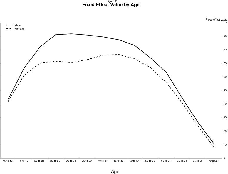
Thus, the age effects are intended to capture the general life-cycle pattern of participation--the average propensity to participate at each age--including the influence of education, fertility, health, and myriad other factors. Figure 7 shows the estimated age effects. The age profiles follow the familiar pattern. Participation rates rise rapidly as young persons leave school. Men, on average, reach their peak participation in their late 20s. The age profile for women pauses at about the same age, dips a bit in the early-30s then rises a bit further to peak in their late 40s, no doubt reflecting fertility patterns. For both sexes, participation begins to fall off rapidly in their 50s.
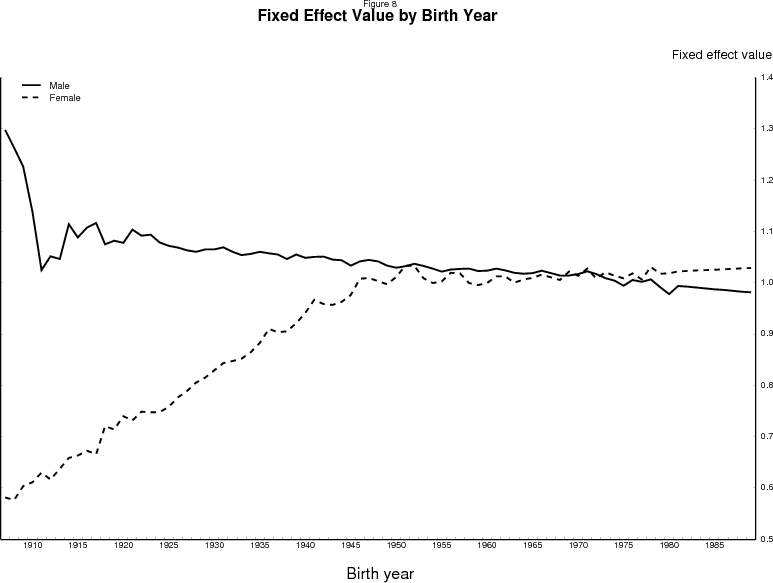
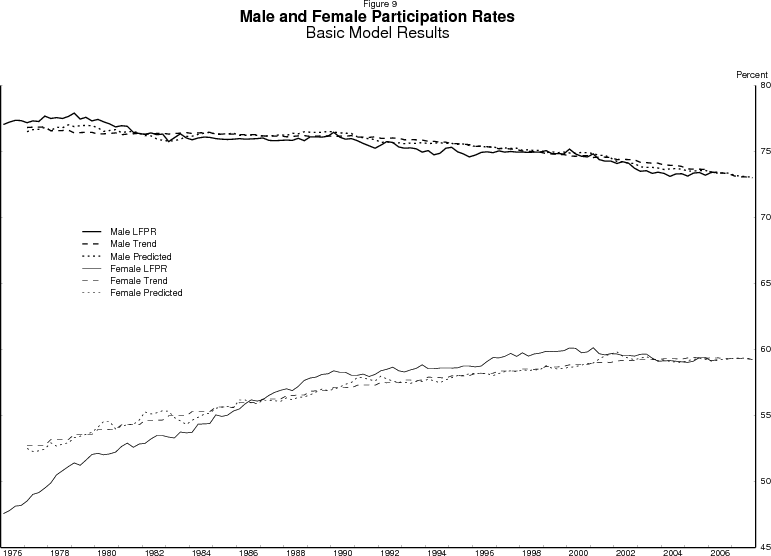
The cohort effects are intended to capture the average propensity of persons born in a particular year to participate over the course of their lives. The estimated cohort effects appear in figure 8. For men, the propensity to participate is estimated to have fallen steadily from cohort to cohort, likely reflecting increasing wealth and ability to finance nonparticipation. These declining cohort effects combine with the movement of the varying-sized cohorts across the age profile from figure 7 to produce a trend for the participation rate of men, shown as the dashed line at the top of figure 9, that falls fairly steadily across our period of analysis.
In contrast, the participation propensities of successive cohorts of women (the dashed line in figure 8) rose rapidly until reaching the cohorts born around 1950, as each generation of women became more likely than their forebears to participate. Since the cohorts born around 1950, however, these propensities have stabilized. Note that this coincides with the inflection points in the actual participation rate series shown in figure 6: The leveling off of the age 35 to 44 and 45 to 54 year old female participation rates occurred about when the 1950 birth cohort was in the middle of these age groups. The pattern of cohort effects interacts with the movement of cohorts across the age profile from figure 7 to produce the aggregate trend for the participation rate of women shown as the dashed line at the bottom of figure 9. This trend rises at a decreasing rate through our analysis period and is close to flat by 2005.
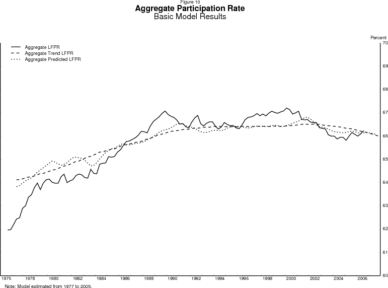
Thus, as figure 9 demonstrates, for men, age and cohort effects alone seem to be able to capture well the basic evolution of the participation rate. For women, age and cohort effects capture the basic evolution of the participation rate in the very broadest terms - rising at a decreasing rate. However, the estimated trend for women clearly fails to reflect the full extent of the curvature in the participation rate of women, and this failure carries over into the aggregate participation rate shown in figure 10. Something is missing for particular age groups of women. In particular, the estimated trends for women in their 20s through their 40s (not shown) exhibit too little "bend," which is why after aggregating by population shares the female trend shown in figure 9 fits the actual data poorly. The participation rates of women in these age groups changed over time in ways not correlated with their birth years. In other words, the female age profile was evolving with time while the basic model assumes it was fixed.9
VII. Evolution of the age and cohort profiles: The enhanced model
The baseline age profile represented by the ![]()
![]() parameters in
equation (4) is assumed to be constant across time. It is intended to capture a basic pattern of life-cycle behavior, and the level of the age effect for any age group is identified by the labor force behavior of the cohorts that appear in that age equation during the sample period. Similarly, the
cohort effects represented by the
parameters in
equation (4) is assumed to be constant across time. It is intended to capture a basic pattern of life-cycle behavior, and the level of the age effect for any age group is identified by the labor force behavior of the cohorts that appear in that age equation during the sample period. Similarly, the
cohort effects represented by the ![]() parameters in (4) are assumed to be constant across time. They are intended to capture the basic propensity of a birth cohort to
participate.
parameters in (4) are assumed to be constant across time. They are intended to capture the basic propensity of a birth cohort to
participate.
As the estimates from the basic model demonstrated, the life-cycle pattern of participation does not appear to have been close enough to constant across cohorts (or time) for that model to be an adequate approximation of reality. Or, equivalently, the relative propensity to participate of a cohort has not been sufficiently constant across ages (or time).10 As various economic and social factors evolved, the age profile of participation evolved as well. The failure of the basic model to capture the curvature in the participation rates of women, in particular, can be attributed to the model's failure to allow cohort profiles or age profiles to evolve. In this section we put forward an "enhanced" model that allows these profiles to change. In doing so, we necessarily blur the analytically convenient distinction between the influence of age and the influence of "era" on participation.
One approach to modeling these changes would be to allow the age effects or the cohort effects to evolve slowly over time according to some predetermined process. However, this method puts a great deal of the weight of identification upon the choice of process, and does not contribute to economic interpretation of the evolution.
Instead, we estimate changes in the shape of the age profiles by including on the right-hand side of the model variables that represent the economic and social changes that we suspect have been, or are likely to be, of greatest significance. That is, we amend the basic model to include more than
just the cyclical controls in the ![]() vector. Thus, equation (4) is replaced by
vector. Thus, equation (4) is replaced by
again suppressing the sex subscripts, where now the variables in the vector ![]() can vary by age group (
can vary by age group (![]() as well as time. Altogether, we estimate 322 parameters in 28 equations.
as well as time. Altogether, we estimate 322 parameters in 28 equations.
We continue to assume that conditional on the variables in ![]() , the age and cohort effects are constant over time. However, these effects now have a different character: The additional
variables mean that the age and cohort effects by themselves will no longer fully describe how participation rates evolve as a person ages or across cohorts. Put differently, the age or cohort effects will no longer fully describe the age or cohort profiles of participation; these
profiles will now also depend upon the variables in
, the age and cohort effects are constant over time. However, these effects now have a different character: The additional
variables mean that the age and cohort effects by themselves will no longer fully describe how participation rates evolve as a person ages or across cohorts. Put differently, the age or cohort effects will no longer fully describe the age or cohort profiles of participation; these
profiles will now also depend upon the variables in ![]() . The age effects themselves may be viewed as defining a baseline or average age profile from which particular cohorts deviate in
accordance with the
. The age effects themselves may be viewed as defining a baseline or average age profile from which particular cohorts deviate in
accordance with the ![]() variables, or as residuals that pick up the life-cycle pattern that we have failed to capture through the included variables. Similarly, the cohort effects may be viewed
as defining the fundamental propensity of a cohort to participate, from which that cohort may deviate at particular ages in accordance with the
variables, or as residuals that pick up the life-cycle pattern that we have failed to capture through the included variables. Similarly, the cohort effects may be viewed
as defining the fundamental propensity of a cohort to participate, from which that cohort may deviate at particular ages in accordance with the ![]() variables, or as residuals that pick up the
influences on the cohort that we have failed to measure with the included variables, i.e., a persistent residual that is constant across time and age. In either case, full age or cohort profiles, of the sort shown in figure 7 and figure 8 for the basic model, will need to include both the age or
cohort effects and the relevant variables, and it will no longer be possible to decompose the trend in participation into disjoint age and cohort components.
variables, or as residuals that pick up the
influences on the cohort that we have failed to measure with the included variables, i.e., a persistent residual that is constant across time and age. In either case, full age or cohort profiles, of the sort shown in figure 7 and figure 8 for the basic model, will need to include both the age or
cohort effects and the relevant variables, and it will no longer be possible to decompose the trend in participation into disjoint age and cohort components.
The condition that the variables in ![]() may vary by both age and time is quite general. In the cases of some of the variables we will discuss momentarily, such as educational attainment, the
variable is constant across time within a cohort - it "ages" with the cohort, so to speak - but varies across cohorts. While in others, such as marriage rates, the variable varies over time or age within a cohort, as well as varying across cohorts.
may vary by both age and time is quite general. In the cases of some of the variables we will discuss momentarily, such as educational attainment, the
variable is constant across time within a cohort - it "ages" with the cohort, so to speak - but varies across cohorts. While in others, such as marriage rates, the variable varies over time or age within a cohort, as well as varying across cohorts.
Note that the coefficients on each variable in ![]() vary freely by age/sex group, except where we have imposed our prior that the coefficient be zero. Because the coefficients differ across
age groups, movements in the variables over time change the shapes of the age profiles even in those cases where the variable itself does not vary by age group.
vary freely by age/sex group, except where we have imposed our prior that the coefficient be zero. Because the coefficients differ across
age groups, movements in the variables over time change the shapes of the age profiles even in those cases where the variable itself does not vary by age group.
The included variables fall into three broad categories: human capital, retirement financing, and family structure. We will discuss each in turn, as well as one category - immigration - that we did not include.
There is a good a priori case to be made for each of the variables we discuss (and others that we do not) to have a significant and independent effect on labor force participation, that is, a good case for including each of them in the model. However, many of these variables have shared broad patterns of movement over our sample period. Indeed, several are largely monotonic: Life expectancies, dependency ratios, and educational attainment have mostly risen over time; fertility and the frequency of defined-benefit pensions have mostly fallen. The series do exhibit variation that will facilitate identification. Even life expectancies are not completely smooth and exhibit non-linear variation, and educational attainment accelerated for the cohorts eligible for the Vietnam era draft, then flattened out and more recently, for women in particular, attainment has picked up again. However, because many important economic influences have trended similarly over the last three decades, choosing which variables to include and in just what fashion is largely a matter of judgment, and the coefficients on the relatively few included variables must be interpreted cautiously. The estimated coefficients from our preferred specification of the enhanced model appear in table 1.
A. Human capital
a. Return to education. The first human capital variable we include in the model is an estimate of the return to a college education relative to a high school education. This variable is constructed from a regression of wages on a standard set of variables that includes different levels of schooling, as in Aaronson, Park, and Sullivan (2006).11 We included separate estimates of this return for men and for women in the equations for school-aged groups (16-17, 18-19, and 20-24). We expected that a higher return to education would be induce more intensive schooling, and thus reduce labor force participation. This proved true for men, but not for women. In fact, the coefficients for school-aged women were significantly positive for the 18-19 and 20-24 age groups. Our interpretation of this perverse result is that for women in these age groups, the increases in the return to a college education reflected more general improvements in the labor market opportunities of women, and they responded by increasing their participation, perhaps even while in school.
b. Educational attainment. A second education variable is the percentage of a cohort who had a college degree at age 27, an age by which most people have completed their formal educations. 12 A comparable variable for high school attainment moved too closely with college attainment to include both in the model.13 For age groups past school-age, educational attainment can be expected to increases the opportunities for and returns from employment, which has both substitution and income effects on labor force participation. We would expect the substitution effect to raise participation, while the higher incomes available to cohorts with more education make them likely to retire earlier, or may enable more intermittent labor force attachment.
For men, college attainment is by and large associated with lower rates of participation, suggesting that the income effect dominates in most age groups. For the oldest persons, however, a greater prevalence of college attainment is associated with higher rates of participation, presumably reflecting the greater suitability for the oldest ages of the types of jobs that a college education makes possible.
For women, the pattern is mixed, with a greater prevalence of college attainment associated with greater labor force participation at some ages and less participation at other ages. We are reluctant to attach structural interpretations to these coefficients. For women, the rise in college education in the model likely represents several developments in labor market opportunities for women that moved in rough tandem with the increases in educational attainment.
c. Minimum wage. For the youngest group (16-17 years old) we also included a variable for the real value of the federal minimum wage. This coefficient on this variable is significantly negative for teenage women but estimated to be close to zero for teenage men.
d. Female/male earnings ratio. Another variable that we considered including under the category of human capital is the ratio of median weekly earnings for full-time working women to those of full-time men. We tried including this variable in the equations for women aged 18-61 (that is, above typical high-school age but below typical retirement ages) in order to represent another aspect of the expansion of women's labor market opportunities, which would be expected to draw more women into the work force and perhaps reduce the degree of specialization into market and home production within the household.14 However, the inclusion of this variable neither improved the fit of the model nor facilitated (as hoped) the interpretation of the coefficients on the educational attainment variables, so we did not include it in our preferred specification.
B. Financing retirement
The labor force participation of older persons can be expected to depend, in part, on their ability to finance retirement. Cohorts that find themselves better positioned to retire at an earlier age will have lower rates of participation in the older age groups. Aside from education, which we treated above, several factors would appear to be among the most likely to affect the ability to finance retirement.15
a. Parameters of the Social Security program. The four most important changes to the Social Security retirement system in our sample period have been to the earnings test, the early retirement rules, the retirement age, and the delayed retirement credit. We summarize the latter three developments by including two variables for the average fraction of the Primary Insurance Amount (PIA) a man would receive if he were to retire at a particular age. One variable is used for the 62-64 age group, and a higher value is equivalent to a smaller penalty for retiring early. The other is used for the 65-69 age group, and a higher value of the variable implies a greater reward for delaying retirement. The coefficients on these two variables have the expected signs, with a smaller penalty for retiring early lowering participation among 62-64 year old men, and a greater reward for retiring later raising participation among 65-69 year old men. Changes to the earnings test during this period coincided with the changes in the delayed retirement credit, so the estimates may reflect some influence of this change although we did not include a separate variable for them.
We tried these variables in the equations for older women. However, the coefficients were never statistically significant and their signs and magnitudes made little sense. This may be because the participation rates of women over most of our sample period are already so low by the ages at which these parameters would be most relevant, leaving little room for the changes in the Social Security program to make an estimable difference. If so, then these program parameters may play more of a role in the years ahead as more women may be nearer to the line between participation and nonparticipation at these older ages.
b. Private pension plans. Large changes have taken place in the coverage and character of private pension plans as well. As is well known, the percentage of workers covered by defined benefit pension plans has been declining for some time, while the incidence of defined contribution plans has been rising.16 DB pension plans tend to provide strong incentive for covered workers to remain at work until a particular date or age, and then incentive for them to retire, while DC pensions tend to be more neutral towards the date of retirement. As a result, we might expect the changing composition of private pensions to affect labor force participation rates at various ages. We tried variables for both the level and the proportion of DB coverage, but found no significance for these variables in our model. We left them out of our preferred specification.
c. Life expectancy. In any forward looking model of labor supply in which workers do not rely entirely upon Social Security or private defined-benefit pensions to finance their retirement, or where the values of those benefits are fixed in nominal terms, we would expect a longer expected lifespan to increase the number of years a person chooses to work, in order to save more for the longer expected retirement and to reduce the number of years of retirement that need to be financed. We expect these extra years to primarily take the form of later retirement. We do not expect persons in prime working years to be near this margin; and it is our considered opinion that young people, who may, in principle, choose to begin working sooner or increase their schooling in anticipation of a longer life, do not, in fact, give much thought to the far future. In addition, to the extent that life expectancy is correlated with better health more generally, longer life expectancies should imply that older individuals would be physically able to work longer into their lives.
We include a variable for gender-specific life expectancy as of age 65, calculated from life tables published by the Census Bureau,17 in the equations for ages 62 and above. Greater life expectancy is associated with higher rates of labor force participation for men and women in the three oldest age groups (although not statistically significantly so for the 65-69 age group of women).
d. The age distribution of the population. The prospects for the generosity of the Social Security system and of private pensions plans depends in large part on the ratio of potential retirees to likely workers, and it is the current and impending increases in this ratio that drive the current concerns about the future of Social Security and Medicare. Accordingly, we used Census Bureau estimates and projections to construct a "potential dependency ratio", defined as the ratio of the population over age 64 to the population age 25-64 that a cohort saw or can expect to see at age 65. However, we found that this variable did not add to the power of the model once the variable for life expectancy was included, and so we did not include it in the specification presented here.
e. Private wealth. For many persons, private wealth, including both financial assets and housing wealth, play an important role in financing retirement. Therefore, one might expect the level of a private wealth to influence the timing of retirement. Indeed, a popular explanation offered for the increase in the labor force participation of older persons following 2000, while the participation rates of other age groups were falling, was that the decline in stock prices, especially to expectations formed during the long bull market, had induced many to delay their retirements. Several researchers have explored the role of wealth in retirement decisions, and suggested that it may be an important element.18 We experimented with several measures of household wealth as explanatory variables in our model, including total household net wealth, stock market wealth, and housing wealth, but found no measures with reasonable explanatory power, even for the age groups near retirement age.
f. Disability benefits. Numerous studies have reported a relationship between SSDI and the long-run downward trend in participation among men. We tried a variable for the disability award rate--the fraction of applications for benefits that were approved in each year--to represent the generosity of the Federal disability insurance program, and, in particular, the changes over time in the stringency of the criteria for being awarded disability benefits. Although this variable is not completely independent of other factors that influence participation--the composition of the applicant pool surely varies with the state of the labor market, for example--it is an improvement in this regard relative to using a measure of disability benefits recipiency. The disability variable did not add significantly to the explanatory power of the model, so we left it out of our preferred specification.
Again, we do not necessarily view the lack of significance of the variables representing private pensions, potential dependency ratios, private wealth or disability benefits as implying that these factors have had no influence on labor force participation in reality. Rather, it is possible that the trends in these variables are being adequately represented by the trends in other elements of the model.
C. Family structure.
We attempt to capture influences associated with family structure with two variables and their interaction in the equations for women.
a. Marriage. At most ages, the percentage of women who are married has fallen substantially over our sample period. For obvious reasons, married women have long had lower participation rates than unmarried women, although we recognize that the decline in marriage rates may be both a cause and a result of increased labor force participation. We included a variable for the percentage of women in the age group who are married, for each age group 18-61. We omitted this variable from the 16-17 age group because their marriage rates are too low to be a significant factor in determining their aggregate participation, and from the older age groups because the change in their marriage rates reflects the changing lifespans of men (i.e., declining rates of widowhood) rather than the choice of family structure, and because of the complications marriage introduces for Social Security benefits. As expected, higher rates of marriage are strongly associated with lower labor force participation rates among women.
b. Fertility. In the equations for women aged 18-29 we included a variable for the percentage of the cohort that, when in each age group, had children younger than 6 years old.19 We expected higher values for this variable to be associated with lower rates of labor force participation. We failed to find this effect at first--indeed, the coefficients on the child variable were significantly positive for two of the age groups--but an interesting pattern emerged when we include an interaction term between the marriage variable and the variable for young children. Taken at face value, the coefficients indicate that for married women in these age groups, the presence of young children is associated with lower rates of labor force participation, but the opposite is true for unmarried women. Obviously we are not estimating an individual-level relationship with our aggregate data, but the results are easily interpreted this way.
One may expect the influence of the presence of young children on labor force participation to have changed over time in response to changing social norms, institutions, and economic opportunity. If so, then it would be desirable to allow the coefficients on the fertility variable to vary over time. For reasons of identification, allowing the coefficient to vary freely is not possible, and simply constraining the coefficients to vary "slowly" over time seemed to us too ad hoc. Instead, we used individual-level data from the CPS to estimate separately for each year an age-group-specific coefficient on a variable for the presence of children less than 6 years old from a cross-section regression of participation.20 We then interacted these coefficients, which vary by year, with the fertility variable in our model. In this way, the coefficient on the fertility variable was constrained to evolve over time in the same way as the cross-sectional coefficients. However, these interactions did not add to the explanatory power of the model, and we did not include them in our preferred specification.
D. Immigration
Another influence on labor force participation is immigration. Because many immigrants come to a new nation in order to find work, we might expect immigration to raise participation rates for some groups. Unfortunately, few good sources of data exist on the foreign born by age. We constructed variables representing the share of foreign born in each age/sex group from data from the decennial censuses and from the CPS. These variables did not influence the aggregate model estimates and had little influence on the individual trends. Moreover, for the most part the coefficient estimates for men were negative--a particularly counter-intuitive result. We therefore excluded these variables.
Immigration also has the potential to influence the population shares. For example, unmeasured immigration may have shifted the population distribution toward age groups with high participation rate without being captured in the government's population estimates. However, the influence of such missing persons is likely small in the aggregate. For example, if one holds within-group participation rates constant and adds a hypothetical 100,000 persons per year in unmeasured immigration since 2002 to the population estimates for 25-29 year old men (who participate with more than 90 percent likelihood), this would raise the level of the participation rate by less than one-tenth percentage point.21
VIII. Results from the enhanced model
As described in section V, we use a measure of the deviation of employment from trend, and two lags, to control for the business cycle. The elasticity of the participation rate with respect to this employment gap for each demographic group (summarized by summing the coefficients) are shown in table 2. For both sexes, the youngest group (those 16 and 17 years old) is by far the most sensitive to the business cycle. Beyond that, among men participation rates are most cyclically sensitive for the youngest and oldest age groups, while the middle age groups (35-59) display relatively little sensitivity. For women, the estimated cyclical sensitivity remains fairly high through their mid forties, but the estimates suggest that women's participation is countercyclical in their late 50s and early 60s.
The relative importance for the historical evolution of the aggregate labor force participation rate of the various other explanatory variables described in section VII depends not only on their estimated coefficients, but also on the extent of variation in each of the variables during our sample period. In order to provide a sense of this, table 3 presents the estimated effect of a one standard deviation increase in each variable on the aggregate trend participation rate. For this illustration, we used 2005 population weights to aggregate the estimates from the 28 separate equations.
Of the included variables, variation in the marriage rate is estimated to have had by far the largest influence on the historical trend, as the increases in participation have coincided in recent decades with the tendency of more couples to postpone marriage or forgo marriage altogether. Indeed, the decline in marriage rates slowed in the years around 1990, at about the same times that female participation rates stopped their rapid ascent. Aside from marriage and its interaction with young children, life expectancy and college attainment are estimated to have had the largest impact on the aggregate rate. Note, however, that although the model estimates that longer life expectancies have raised participation by raising within-group participation rates, that estimate does not incorporate the effect of the corresponding increase in the relative number of elderly individuals, which would put downward pressure on the trend. Note also that although changes in the social security program are estimated to have had, on net, relatively little influence, they are more important within the narrow age groups where these variables are relevant.
As we emphasized above, in the enhanced model the age and cohort effects do not fully represent the age and cohort profiles, that is, how average participation rates evolve over the life-cycle or across cohorts. Instead, age or cohort profiles must include both the age or cohort effects and the influence of the time-varying variables, except those that capture cyclical changes in participation.
To construct cohort profiles, we calculate the trend participation rate for each age group in each year as
The age profiles are computed in a similar fashion, except that the contributions of the cohort effects are omitted from the calculation to remove the direct effects of the changing mix of cohorts in an age group over time. In principle, for each birth cohort we could trace out the trend as we move from age group to age group. For purposes of presentation, however, we aggregated into five-year groups of cohorts.
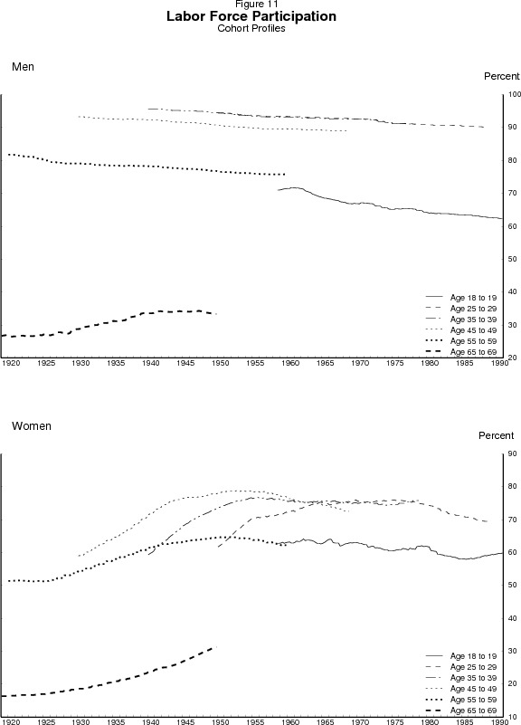
Figure 11 shows the cohort profiles for selected age groups. For men, the cohort profiles are generally declining, as successive cohorts have lower propensities to participate in the labor force than their predecessors in each age group, with the notable exception of the oldest age group. Individuals in this oldest group (which begins with cohorts born in the late 1920s) exhibit an increasing propensity to participate that no doubt reflects greater expected longevity and better health rather than a latent increasingly favorable attitude towards work at retirement age. Women share this feature at ages 65 and over. In addition, teenage women, like teenage men, have been, by and large, increasingly less likely to participate in the labor force. In the middle age groups, however, successive cohorts of women display higher participation rates to a point, then peak and in the turn down.
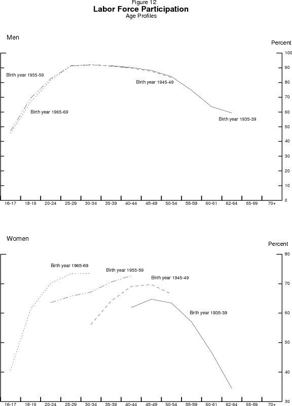
The age profiles in figure 12 are shown for selected groups of birth cohorts that are well represented in those age groups in order to highlight how those profiles have evolved over time. The profiles for men have been remarkably stable. As can be seen in the upper panel, the age profile segments for the various groups of birth cohorts lie on top of each other for those ages for which they overlap, suggesting that a single age profile applies to all cohorts in the sample. In contrast, the age profiles for women (in the lower panel) are disjoint, suggesting that they have evolved significantly over time. Most notably, more recent cohorts appear to have reached their peak rates of participation earlier in life: Participation rates of the oldest cohorts shown - those born in the 1930s - apparently peak in their late 40s, while rates for those born in the late 1940s peak in their early 40s, and the rates for those born in the late 1960s seem likely to be peaking in their early 30s.
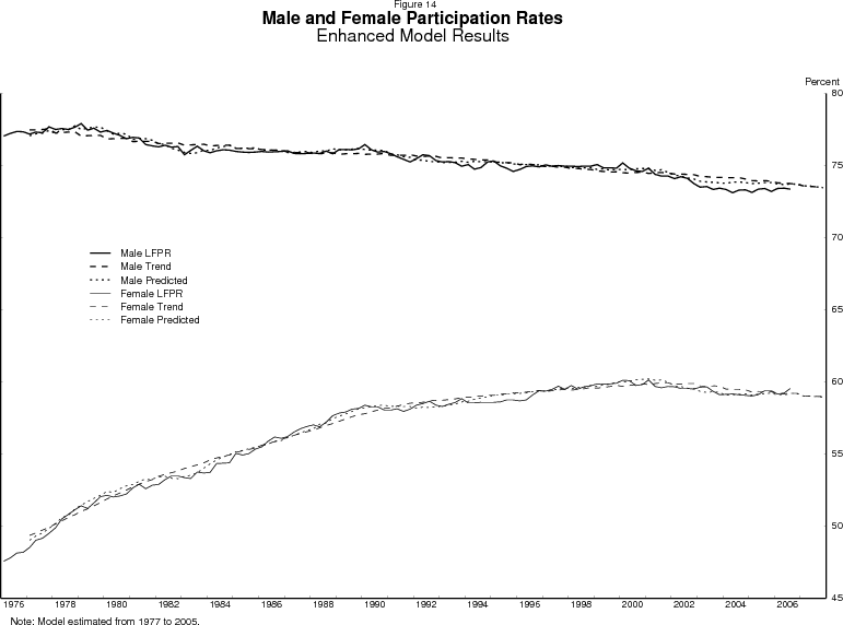
Figure 13 shows the enhanced model's estimated trend for the aggregate labor force participation rate. The model appears to fit the aggregate participation rate rather well. The aggregate trend follows the familiar pattern of rising then flattening, and the enhanced model captures the bend that the basic model missed. The trends for men and women are shown separately in figure 14.
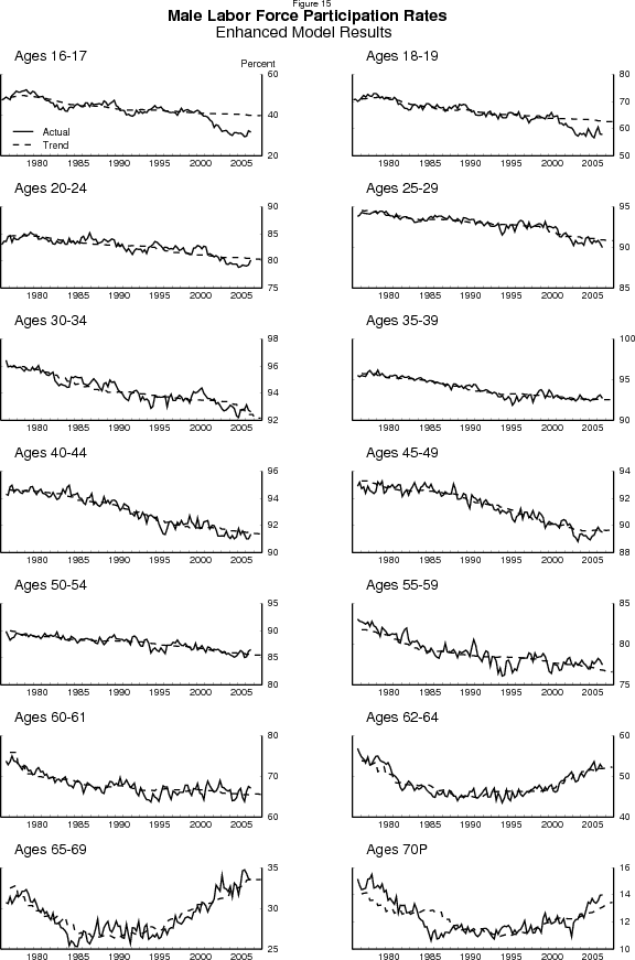
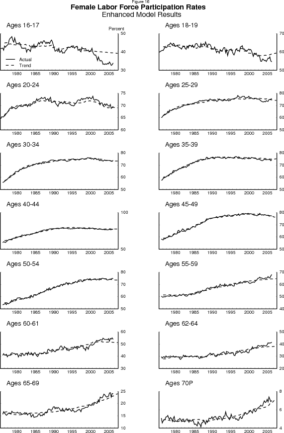
Figures 15 and 16 show the actual participation rates and the estimated trends for each of the 28 age/sex groups. By and large, the model captures the movements in the participation rates of the various groups quite well. There are isolated periods - such as 1994-5 for middle-aged men and 1984-5 for older men - where the model fails to capture the group's behavior. But we are more concerned about the model's estimates for older persons and teenagers over the past few years, to which we return below.
IX. Recent movements in the participation rate
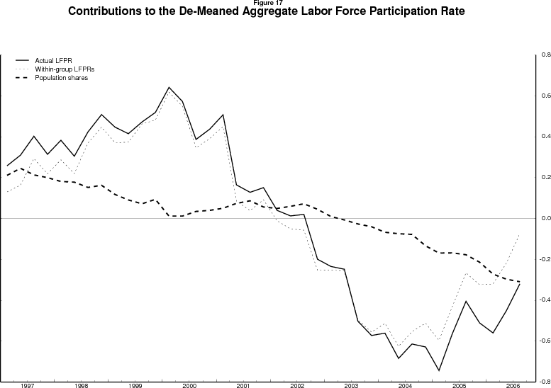
The solid line in figure 17 shows the aggregate labor force participation rate relative to its mean (that is, the left-hand side of equation (1)), from 1997 to midway through 2006. The participation rate first rose as the labor market continued to tighten, then began to fall sometime early in 2000. The participation rate continued to fall into early 2005, well after the labor market had begun to improve, before rising through the latest data shown. These persistent declines in participation during a labor market expansion caused many analysts to ask whether this behavior reflected trend or cycle.
The dark and light dashed lines repeat the decomposition from equation (1) for this shorter period, this time aggregating across the age/sex groups to show the total contributions of shifting population shares (the aging of the population) and of within-group changes in participation rates. During the late 1990s period of labor market tightening, the two forces worked in opposite directions, with aging modestly damping the presumably cyclical increases in within-group participation rates. From 2000 to 2002, including the recession and its immediate aftermath, aging was a neutral factor while presumably cyclical decreases in within-group participation rates drove the aggregate rate down. Looking back at figure 13, the model tells a more nuanced story: Virtually all of the movements in the aggregate participation rate between 1997 and 2002 were cyclical movements about a fairly flat trend, as the net downward pressure on the trend from population aging was offset by continued upward movement in the trends for some demographic groups.
In contrast, since 2002 the movement (or lack thereof) in the aggregate participation rate has been a cyclical recovery back towards a declining trend. The model suggests that the aggregate trend rate dropped from 66.8 percent to 66.2 percent between the fourth quarter of 2002 and the fourth quarter of 2006. Why? Roughly two-thirds of this decline - about 0.4 percentage point - is due to shifting demographic shares, especially the redistribution of baby boomers from high participation rate ages to low participation rate ages. The remainder is due to a combination of developments. On the one side, the flattening of women's trend participation in prime-aged groups combined with the ongoing decline in men's trend participation in prime and younger age groups to push the aggregate participation rate down. One the other side, the model estimates that the trends for the participation rates of men and women aged 62 and over are rising, and these rising trends among older individuals offsets some of the downward pressure from the younger age groups.
As we mentioned at the end of the previous section and show in figures 15 and 16, there are a few groups for which the model cannot explain recent developments well. Women from age 55 to 64 and men in the oldest age group have had participation rates persistently above trend for the past few years. The model does explain significant increases in the trend participation rates of older persons of both sexes beginning in the mid-1990s as a function of rising life expectancies and changes in the Social Security rules. But the recent increases among these groups are larger than the model can explain.23 Although they may become more important as time goes on, for now the gaps between the model predictions for women age 55 to 64 and the oldest men have only a modest influence on the aggregate trend.
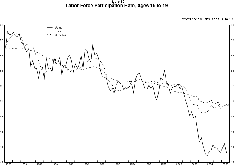
In contrast, the low participation rates of teenagers (16-17 and 18-19) of either sex during the last three years is striking, and influences the aggregate trend more significantly.24 The model's surprise is easily seen in figure 18, where the participation rates of the teenagers of both sexes, their trends, and the corresponding model predictions have been aggregated into one 16-to-19-year-old demographic group. As the dotted line indicates, the model is not surprised that the participation rates for these groups dropped rapidly in the recession. Instead, the model is surprised by the extent of the drop and especially that the participation of teens failed to recover even after employment growth resumed in earnest in 2003.
The decline is puzzling in part because little of it is explained by shifts from market work to school enrollment.25 Even examining the available BLS time use surveys from 2003 to 2005, a period of cyclical recovery in employment, shows that over the two years 16-to-24-year olds reduced both the average hours per day working and the average hours per day in school or school-related activities. In contrast, time spent in personal care and other activities rose noticeably. Minimum wages are also an unlikely culprit. The model already incorporates the real value of the minimum wage, and no discrete change in minimum wages occurred in 2001-2002 to link to the precipitous fall in teenage labor market attachment at that time. More generally, the earnings of younger workers relative to older workers showed no deterioration in the past few years. The low levels of participation among teens remains a puzzle.
X. Conclusion
In this paper we presented a model of the aggregate labor force participation rate that makes several contributions to the literature on labor supply. First, the model provides a trend-cycle decomposition that is an appealing alternative to aggregate time series models and other smoothing algorithms. For example, the Kalman Filter necessarily relies on history to decide how much recent innovation to pass through to trend. Such a filter risks falsely extrapolating historical experience, and in addition, could misidentify cyclical influences at the end of any estimation period. In contrast, the model we proposal abstracts from the cyclical influence of the most recent data, and allows the observed behavior of cohorts identified over full business cycles to project forward future labor force attachment. In addition, the trends estimated in the paper are more directly interpretable in an economic context, as the influence of demographics and cohorts can be deciphered. Thus, although our model also risks falsely extrapolating historical experience, we can point to the assumptions that lead us astray, or test the sensitivity of our model to the underlying assumptions. Arguably, the model we propose thus offers a useful tool for projecting future estimates of labor supply.
Second, the model uncovers several interesting features of aggregate labor supply. In particular, in identifying the patterns among female birth cohorts, the model estimates that female labor force participation rates have leveled off not solely because of contemporaneous developments in the labor market opportunities for women, but also because the increases in the generation-specific attachment of successive cohorts of women in the labor force began leveling off with the cohorts born in the early 1950s. This conclusion is based not on simple extrapolations of recent trends, but on observing these cohorts for 40 years, and their successors through several business cycles. The model thus suggests that, barring major changes in policy or environment, women's labor supply will likely show little further gain in the coming years. Indeed among some age groups, female labor supply has changed direction and is trending down. Entering cohorts of women no longer exhibit substantially more attachment than exiting cohorts, suggesting that this social phenomenon is no longer putting discernable upward pressure on the aggregate rate.
Third, the model can be used to ask many interesting questions that we have not yet explored. For example, with appropriate caution, the model could be used to simulate the changes in future labor supply due to changes in immigration policy or further increases in longevity. The model simulations could also be used to build trends for economic aggregates heavily influenced by labor force participation rates, such as aggregate labor income.
In sum, we developed a model of the labor force participation rate that combines differences in labor force participation across birth cohorts, differences in participation across ages, and the evolution of the age distribution of the population into a unified structure. We introduced a basic model that captures the intuition of how labor force attachment has evolved over the past thirty years, and an enhanced model that captures more nuanced evolution associated with measurable developments in education, family structure, government programs, longevity, and other variables. While the model fits well over most of history for most age/sex groups, there remain anomalies in the past few years - among teenagers and older persons, in particular. Despite these puzzles, the framework we propose for estimating broad trends in labor supply appears to have many potential uses and offer an interesting line of research.
Aaronson, Daniel, Kyung-Hong Park, and Daniel Sullivan. 2001. "Growth in Worker
Quality." Economic Perspectives (Federal Reserve Bank of Chicago) 2001(4):53-74.
Aaronson, Stephanie, Bruce Fallick, Andrew Figura, Jonathan Pingle, and William Wascher. 2006. "The Recent Decline in the Labor Force Participation Rate and Its Implications for Potential Labor Supply," Brookings Papers on Economic Activity, (1):69-134.
Baxter, Marianne, and Robert G. King. 1999. "Measuring Business Cycles: Approximate Band-Pass Filters for Economic Time Series," The Review of Economics and Statistics, 81(4): 575-593, November.
Burtless, Gary. 1999. "An Economic View of Retirement." In Behavioral Dimensions of Retirement Economics, edited by Henry J. Aaron. Brookings Institution Press, Washington, D.C.
Bowen, William G., and T. Aldrich Finegan. 1969. The Economics of Labor Force Participation. Princeton University Press, Princeton, New Jersey.
Coronado, Julia L. and Maria Perozek, "Wealth Effects and the Consumption of Leisure: Retirement Decisions During the Stock Market Boom of the 1990s," Finance and Economics Discussion Series #2003-20, Federal Reserve Board, May 2003.
Durand, John D., The Labor Force in the United States 1890-1960. New York: Social Science Research Council, 1948.
Frees, Edward W. 2003. "Stochastic forecasting of labor force participation rates," Insurance: Mathematics and Economics, 33:317-336.
Goldin, Claudia. 2006. "The Quiet Revolution That Transformed Women's Employment, Education and Family." American Economic Review, Papers and Proceedings 96(2):1-21.
Greenberg, B.G., John J. Wright and Cecil G. Sheps. 1950. "A Technique for Analyzing Some Factors Affecting the Incidence of Syphilis," American Statistical Association Journal, September, 373-399.
Gustavsson, Magnus and Par Osterholm. 2006. "The informational value of unemployment statistics: A note on the time series properties of participation rates," Economics Letters, 92(2):428-433.
Hotchkiss, Julie L. 2005. "What's Up with the Decline in Female Labor Force Participation?" Working Paper 2005-18. Federal Reserve Bank of Atlanta (August).
Jaeger, David A. 1997. "Reconciling the Old and New Census Bureau Education Questions: Recommendations for Researchers." Journal of Business and Economic Statistics 15(3): 300-309.
Kirkland, Katie. 2002. "Declining Teen Labor Force Participation," Issues in Labor Statistics, September.
Loughran, David S., and Steven Haider. 2005. "Do the Elderly Respond to Taxes on Earnings? Evidence from the Social Security Retirement Earnings Test." RAND Corporation Labor and Population Working Paper WR-223.
Kominski, Robert, and Paul M. Siegel. 1993. "Measuring Education in the Current Population Survey." Monthly Labor Review 116(9): 34-38.
McNown, Robert and Cristobal Ridao-Cano. 2005. "A time series model of fertility and female labor supply in the UK," Applied Economics, 37:521-532.
Mulligan, Casey B., and Yona Rubinstein. 2006. "Specialization, Inequality, and the Labor Market for Women." Unpublished manuscript. University of Chicago (January).
Pingle, Jonathan F. 2006. "Social Security's Delayed Retirement Credit and the Labor Supply of Older Men," Finance and Economics Discussion Series #2006-37, Federal Reserve Board, August 2006.
Poterba, James, and Joshua Rauh, Steven Venti and David Wise. 2006. "Defined Contribution Plans, Defined Benefit Plans, and the Accumulation of Retirement Wealth," National Bureau of Economic Research, Working Paper #12597, October.
Wachter, Michael L. 1977. "Intermediate Swings in Labor-Force Participation," Brookings Papers on Economic Activity, 1977(2):545-576.

| age | men | men |
women | women |
|---|---|---|---|---|
| 16 to 17 | -0.32 | 0.02 | -0.05 | 0.02 |
| 18 to 19 | -0.17 | 0.01 | 0.64 | 0.10 |
| 20 to 24 | -0.04 | 0.01 | 0.10 | 0.04 |
| age | men | men |
women | women |
|---|---|---|---|---|
| 25 to 29 | -0.09 | 0.04 | -1.38 | 0.24 |
| 30 to 34 | -0.04 | 0.04 | 0.02 | 0.11 |
| 35 to 39 | -0.05 | 0.04 | 0.52 | 0.13 |
| 40 to 44 | -0.07 | 0.04 | 0.54 | 0.33 |
| 45 to 49 | -0.12 | 0.04 | -0.30 | 0.16 |
| 50 to 54 | -0.13 | 0.04 | 0.19 | 0.14 |
| 55 to 59 | -0.14 | 0.05 | 0.25 | 0.15 |
| 60 to 61 | -0.23 | 0.07 | -0.50 | 0.39 |
| 62 to 64 | -1.47 | 0.18 | -1.47 | 0.90 |
| 65 to 69 | -1.16 | 0.29 | 3.07 | 0.93 |
| 70 over | 0.62 | 0.36 | 5.66 | 1.00 |
| age | men | men |
women | women |
|---|---|---|---|---|
| 62 to 64 | 1.22 | 0.13 | 1.57 | 0.57 |
| 65 to 69 | 1.61 | 0.35 | 0.35 | 0.52 |
| 70 over | 2.05 | 0.34 | 1.67 | 0.50 |
| age | men | men |
women | women |
|---|---|---|---|---|
| 16 to 17 | 0.00 | 0.01 | -0.03 | 0.01 |
| age | men | men |
women | women |
|---|---|---|---|---|
| 62 to 64 | -1.82 | 0.18 |
| age | men | men |
women | women |
|---|---|---|---|---|
| 65 to 69 | 3.56 | 0.93 |
| age | women | |
|---|---|---|
| 18 to 19 | -5.25 | 1.76 |
| 20 to 24 | -5.68 | 0.66 |
| 25 to 29 | -1.80 | 0.82 |
| 30 to 34 | -3.77 | 0.11 |
| 35 to 39 | -2.63 | 0.16 |
| 40 to 44 | -1.84 | 0.58 |
| 45 to 49 | -2.82 | 0.30 |
| 50 to 54 | -1.28 | 0.29 |
| 55 to 59 | 0.24 | 0.36 |
| 60 to 61 | -2.60 | 1.29 |
| age | women | women |
|---|---|---|
| 18 to 19 | 0.21 | 0.08 |
| 20 to 24 | 1.09 | 0.14 |
| 25 to 29 | -0.96 | 0.57 |
| age | women | women |
|---|---|---|
| 18 to 19 | -4.72 | 1.15 |
| 20 to 24 | -4.56 | 0.47 |
| 25 to 29 | 1.03 | 1.29 |
| Age (years) | Males Elasticitya |
Males Standard Error |
Females Elasticitya |
Females Standard Error |
|---|---|---|---|---|
| 16-17 | 1.84 | .16 | 1.89 | .16 |
| 18-19 | .25 | .08 | .33 | .13 |
| 20-24 | .42 | .06 | .35 | .08 |
| 25-29 | .14 | .02 | .45 | .09 |
| 30-34 | .16 | .02 | .35 | .04 |
| 35-39 | .04 | .02 | .36 | .05 |
| 40-44 | .07 | .02 | .39 | .07 |
| 45-49 | .06 | .02 | .03 | .06 |
| 50-54 | .06 | .04 | .34 | .07 |
| 55-59 | -.03 | .06 | -.24 | .10 |
| 60-61 | .29 | .12 | -.56 | .21 |
| 62-64 | .47 | .16 | -.47 | .26 |
| 65-69 | .46 | .23 | .16 | .35 |
| 70 and over | .60 | .36 | -.43 | .35 |
Source: Authors' calculations.
a. Sum of the coefficients on the employment gap in the current period and two lags. Return to Table
| Variablea | Percentage points |
|---|---|
| Returns to education | .063 |
| College completion rate | -.137 |
| Life expectancy | .228 |
| Minimum wage | -.002 |
| Generosity of early-retirement rules | -.023 |
| Generosity of delayed retirement credits | .033 |
| Marriage rate | -2.693 |
| Presence of children under 6 in family | .040 |
| Interaction of marriage and children | -1.016 |
Source: Authors' calculations.
a. See the text for definitions of the variables. Return to Table
Footnotes
However, such a formula attributes a positive contribution to aggregate participation to any group whose population share rises, and a negative contribution to any group whose population share falls, regardless of whether the group's participation rate is above or below the average. In contrast, formula (1) takes into account that when the population share of one group rises, that necessarily means that the share of the other groups falls. Return to Text
 g = 1 to 14


