The 'Elusive' Capital-User Cost Elasticity Revisited
Keywords: User cost elasticity, fixed investment, capital accumulation, price of capital, interest rate
Abstract:
JEL classifications: C23, E22, E44, E62
1 Introduction
Economists have long had a keen interest in knowing the degree that businesses wish to adjust capital holdings in response to shifts in the supply of capital--the user cost elasticity of capital. The attention paid to this parameter is well justified, as its magnitude is of central importance for calibrating macroeconomic models that, in turn, are used for forecasting, for evaluating economic hypotheses, and examining fiscal and monetary policy alternatives. For example, this elasticity is relevant for assessing the effectiveness of investment tax incentives, such as the bonus depreciation allowances enacted by the U.S. federal government in 2002, 2003 and 2008. Despite its significance, econometricians have generally found it difficult to identify this elasticity in empirical work, leading to estimates that vary substantially in magnitude from study to study. This reflects the familiar econometric challenge of identifying the slope of a demand curve in an environment where both demand and supply can be shifted by sources that cannot always be isolated.1 This challenge is complicated further in this context by adjustment costs--both internal and external. These costs prolong the period needed for capital to fully adjust to a given disturbance and tend to make the demand response depend on the anticipated persistence of the shock (Tevlin and Whelan [2003]).2
Recently, new methods have been applied to this topic that point to a fairly large aggregate response of capital demand to changes in capital supply. Much of this work has followed from the insights of Caballero [1994], who argued that the user cost elasticity can be identified more effectively using a cointegration approach that emphasizes the low-frequency variation in the data, thereby de-emphasizing transitory distortions associated with adjustment costs and possibly sidestepping endogeneity problems. Using this strategy for aggregate data for equipment capital, Caballero [1994] and Schaller [2006] obtain statistically significant estimates of the long-run user cost elasticity that are close to the Cobb-Douglas benchmark of -1.0.3 However, the estimates in these studies become insignificant when structures are included in the measure of capital. This is not a negligible omission, as structures constitute a huge fraction of the nominal stock of business capital, and therefore should be an important component of the overall response of capital to changes in its user cost.4 More recent work by Smith [2007] uses cointegration methods for a panel of United Kingdom industries, but with a measure of capital that includes both equipment and structures. He finds a user cost elasticity that is substantially smaller-- around -0.40. Using a stationary specification and aggregate data for the United States, Tevlin and Whelan [2003] find estimates of the user cost elasticity around -0.20.
This study revisits the subject using a unique quarterly dataset of manufacturing industries from South Africa for the period between 1970 and 2000. We think that the South African experience over this period is particularly pertinent to the user cost elasticity debate. The country is sufficiently small and open that its economy likely takes interest rates and capital goods prices as given (Schaller [2006]), and is sufficiently isolated that we can conjecture that these prices are also exogenous. This allows us to bypass some of the challenges posed by endogeneity. Also, our industry level dataset has a large number of observations and a cross-sectional dimension, which allows us to control for sources of endogeneity stemming from latent aggregate and industry effects and may make our results less susceptible to small sample bias than some previous studies. Finally, the embargo imposed on South Africa provides a unique opportunity to assess the importance of endogeneity for estimates of the user cost elasticity since the embargo forced the country's economy to transition from open toward autarky, and then back to open. Under our working assumption that the user cost is exogenous in a small and isolated open economy, we would expect the user cost elasticity to be smaller during the embargo period-- when the endogeneity problem was likely more severe--than in the non-embargo periods.
Using both cointegration and distributed lag specifications that are derived directly from optimal investment behavior in the presence of adjustment costs, we find highly significant estimates of the user cost elasticity in the range of -0.80 to -1.0. In most cases, these estimates are statistically indistinguishable from the Cobb-Douglas benchmark of ![]() . Unlike previous studies (Caballero [1994] or Schaller [2006]) that also find user cost elasticity estimates in this range, our estimates are for
measures of business fixed capital that includes both equipment and structures. To our knowledge, this study is one of the first to document such a large user cost elasticity for a broad measure of business capital that includes both equipment and structures, and the first to show that similar
estimates can be obtained using both stationary and cointegrating regression specifications. Interestingly, we find that controlling for the effect of the embargo period-- when the economy was less open and more likely to have interest rates and prices of capital goods that are determined
endogenously-- leads to a statistically significant increase in the absolute value of the user cost elasticity estimate. The estimated elasticity during the embargo period is much smaller, in the range of estimates found in the majority of previous studies. These latter results are particularly
intriguing as they suggest the importance of endogeneity as a possible explanation for why previous studies--which largely employ data from large economies--have often failed to obtain estimates of the user cost elasticity of a substantial magnitude.
. Unlike previous studies (Caballero [1994] or Schaller [2006]) that also find user cost elasticity estimates in this range, our estimates are for
measures of business fixed capital that includes both equipment and structures. To our knowledge, this study is one of the first to document such a large user cost elasticity for a broad measure of business capital that includes both equipment and structures, and the first to show that similar
estimates can be obtained using both stationary and cointegrating regression specifications. Interestingly, we find that controlling for the effect of the embargo period-- when the economy was less open and more likely to have interest rates and prices of capital goods that are determined
endogenously-- leads to a statistically significant increase in the absolute value of the user cost elasticity estimate. The estimated elasticity during the embargo period is much smaller, in the range of estimates found in the majority of previous studies. These latter results are particularly
intriguing as they suggest the importance of endogeneity as a possible explanation for why previous studies--which largely employ data from large economies--have often failed to obtain estimates of the user cost elasticity of a substantial magnitude.
2 The Embargo: Some Background
As mentioned above, a key feature of the South African economic history that we exploit in this study is the country's unique revision toward autarky that began around 1985 and ended early in 1994. During this period, the world imposed economic sanctions on South Africa to encourage an end to its apartheid regime--a political system that granted different rights to citizens based on race. As a result of the embargo, several foreign public and private entities operating in South Africa decided to disinvest and/or stop making new investments or reinvestments of earnings in the country.5 In addition to these restrictions on capital flows, several countries also restricted or banned trade with South Africa. These restrictions limited the country's ability to trade goods and financial claims with the rest of the world.
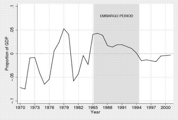
South Africa's trade-to-GDP ratio dropped from an average of 23 percent during the pre-embargo period to an average of 19 percent during the embargo, then snapped back to an average of 25 percent after the embargo was lifted. The country's current account balance, shown in Figure 1, also follows a pattern consistent with these restrictions.6 Before 1985, the country registered current account deficits that averaged 2 percent of GDP. However, when economic sanctions intensified between 1985 and 1993, the current account balance swung to a surplus that averaged about 2.4 percent of GDP. When economic sanctions were lifted in early 1994, the current account balance reversed again to a deficit as the country re-integrated into the world economy.7
For estimation purposes, we interpret the beginning of the embargo as September 1985, when official sanctions were enacted against South Africa by the European Community and the United States, and the end of the embargo as April 1994, when the country held its first all-race democratic elections.8 These dates are also consistent with the swings in South Africa's current account balance discussed above.
3 Theoretical Motivation
We assume that each industry can be represented by a forward-looking representative firm that operates in perfectly competitive markets and that faces internal costs for adjusting its capital stock. Each of these firms maximizes its market value by choosing its labor input for the current period and its capital stock for the following period. The investment decision balances costs of adjustment against the costs associated with deviating from capital holdings that would be optimal in the absence of internal adjustment costs. As a preliminary step, we define frictionless capital as:
![\displaystyle k_{i,t}^{\ast}\equiv y_{i,t}-\sigma u_{i,t}+\left( \sigma-1\right) a_{i,t}^{k}=\left[ \begin{array}[c]{ccc}% 1 & -\sigma & \left( \sigma-1\right) \end{array} \right] \left[ \begin{array}[c]{c}% y_{i,t}\\ u_{i,t}\\ a_{i,t}^{K}% \end{array} \right] %](img6.gif) |
(1) |
for industries
![\displaystyle U_{i,t}=p_{i,t-1}^{K}\left( \frac{1-\tau z_{t}}{1-\tau}\right) \left[ r_{t-1}^{f}+\zeta+\delta_{i}-\frac{E_{t-1}\left[ \Delta p_{i,t}^{K}\right] }{p_{i,t-1}^{K}}\right]](img19.gif) |
(2) |
where
We assume that the determinants of
![]() in equation (3) in each industry evolve according to a joint stochastic process that competitive firms treat as given.11 A key issue for identification is whether there is capital-augmenting technological progress so that
in equation (3) in each industry evolve according to a joint stochastic process that competitive firms treat as given.11 A key issue for identification is whether there is capital-augmenting technological progress so that
![]() shows up as a determinant of
shows up as a determinant of
![]() . Our specification allows for technology to have independent effects on all factors of production, thereby nesting as special cases a number of important alternatives. One
special case is Hicks-Neutral technological progress, where a common technological factor
. Our specification allows for technology to have independent effects on all factors of production, thereby nesting as special cases a number of important alternatives. One
special case is Hicks-Neutral technological progress, where a common technological factor
![]() augments all inputs to the same extent. A second important special case is for technology to solely augment labor so that
augments all inputs to the same extent. A second important special case is for technology to solely augment labor so that
![]() . As King, Plosser, and Rebelo [1988] show, this case is theoretically appealing because it allows for the existence of a balanced growth steady state.
A third possibility is that production takes a Cobb-Douglas form, which imposes the restriction that
. As King, Plosser, and Rebelo [1988] show, this case is theoretically appealing because it allows for the existence of a balanced growth steady state.
A third possibility is that production takes a Cobb-Douglas form, which imposes the restriction that ![]() so that the final term involving the unobserved technology factor drops out of
equation (3). A final, more general, possibility is a case where both capital- and labor-augmenting technology are allowed to have distinct trajectories.
so that the final term involving the unobserved technology factor drops out of
equation (3). A final, more general, possibility is a case where both capital- and labor-augmenting technology are allowed to have distinct trajectories.
We assume that the representative firm in each industry ![]() seeks to maximize the present value of its cash flows by choosing optimal trajectories of capital and labor in the face of
adjustment costs for capital:
seeks to maximize the present value of its cash flows by choosing optimal trajectories of capital and labor in the face of
adjustment costs for capital:
![\displaystyle % {\displaystyle\sum\limits_{j=0}^{\infty}} R_{t}^{t+j}E_{t}\left\{ \left( 1-\tau_{t+j}\right) \left\{ F\left( K_{i,t+j},L_{i,t+j}\right) -w_{i,t+j}L_{i,t+j}\right\} -\overline{p}% _{i,t+j}^{k}\left[ I_{i,t+j}+J\left( K_{t+1+i},...,K_{t+1+i-M}\right) \right] \right\} %](img31.gif) |
(3) |
where the optimization is subject to the capital accumulation constraint
 is the real price of capital after deducting the present value of capital depreciation allowances.
In Appendix 6, we generalize the approach described in Tevlin and Whelan [2003] to show that, up to a linear approximation, the optimal capital stock will follow a distributed lag of the form:
![\displaystyle k_{i,t+1}=\left[ \begin{array}[c]{ccc}% 1 & -\sigma & \left( \sigma-1\right) \end{array} \right] G(B)\left[ \begin{array}[c]{c}% y_{i,t}\\ u_{i,t}\\ a_{i,t}^{K}% \end{array} \right] %](img47.gif) |
(5) |
where
In this model, the potential presence of the unobserved factor
![]() means that cointegration between capital, output and the user cost may not hold in general, but may hold for the special cases (discussed above) in which this term
disappears.15 If cointegration does hold, then a levels specification could be a particularly efficient identification strategy because the estimated
parameters from this regression are super-consistent even in the presence of endogeneity. However, if cointegration fails to hold, then estimates using levels specifications could yield spurious results.16 We regard the potential presence of such a relationship as an empirical issue, and test the null of no cointegration using formal panel cointegration tests. In addition, we estimate the user cost elasticity using difference
specifications that do not rely on cointegration.
means that cointegration between capital, output and the user cost may not hold in general, but may hold for the special cases (discussed above) in which this term
disappears.15 If cointegration does hold, then a levels specification could be a particularly efficient identification strategy because the estimated
parameters from this regression are super-consistent even in the presence of endogeneity. However, if cointegration fails to hold, then estimates using levels specifications could yield spurious results.16 We regard the potential presence of such a relationship as an empirical issue, and test the null of no cointegration using formal panel cointegration tests. In addition, we estimate the user cost elasticity using difference
specifications that do not rely on cointegration.
As one would expect, identification in these specifications hinges on our ability to isolate exogenous movements in the user cost while controlling for changes in output--the relevant shift factor for demand. We think that our South African data may be particularly useful in this regard, because the user cost is likely to be exogenous during the non-embargo portion of our dataset. Taken together, estimates using these alternative approaches should provide a fairly robust sense of the range of elasticity estimates that can be supported by the data.
4 Data
Our dataset consists of a quarterly panel of 24 two-digit manufacturing industries over the period from 1970:Q1 to 2000:Q4.17 Quarterly industry-level
estimates of the real capital stock (![]() ), fixed investment, gross value added (
), fixed investment, gross value added (![]() ), consumption of fixed capital, and industry-specific price deflators for investment (
), consumption of fixed capital, and industry-specific price deflators for investment (
![]() ) and output (
) and output (
![]() ) were obtained from South Africa Trade and Industrial Policy Strategies (TIPS). Quarterly data for prime borrowing rates (
) were obtained from South Africa Trade and Industrial Policy Strategies (TIPS). Quarterly data for prime borrowing rates (![]() ) and the average corporate tax rate (
) and the average corporate tax rate (![]() ) were obtained from the South African Reserve Bank. The user cost of capital for
each industry in each quarter (
) were obtained from the South African Reserve Bank. The user cost of capital for
each industry in each quarter (![]() ) was calculated using equation (3). The cost of capital component of the user cost (the bracketed term in the user cost
equation) is calculated as the sum of the nominal borrowing cost in the preceding quarter (
) was calculated using equation (3). The cost of capital component of the user cost (the bracketed term in the user cost
equation) is calculated as the sum of the nominal borrowing cost in the preceding quarter (![]() ), a fixed risk premium of 10 percentage points, the estimated depreciation rate (
), a fixed risk premium of 10 percentage points, the estimated depreciation rate (
![]() ), less a proxy for anticipated capital gains for investment goods (
), less a proxy for anticipated capital gains for investment goods (
![]() ) in that quarter.18 For each industry, we proxy for expected capital gains using the conditional forecast from an OLS regression that projects the four-quarter rate of increase in the investment price deflator onto variables in the time
) in that quarter.18 For each industry, we proxy for expected capital gains using the conditional forecast from an OLS regression that projects the four-quarter rate of increase in the investment price deflator onto variables in the time ![]() information set: Namely, current and lagged values of the nominal interest rate and lags of the dependent variable.19 The capital price component of the user cost (
information set: Namely, current and lagged values of the nominal interest rate and lags of the dependent variable.19 The capital price component of the user cost (
![]() ) is formed as the ratio of the industry's investment deflator and its output deflator, and is multiplied by our estimates of the relevant tax terms.20
) is formed as the ratio of the industry's investment deflator and its output deflator, and is multiplied by our estimates of the relevant tax terms.20
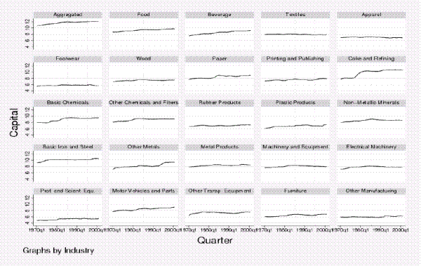
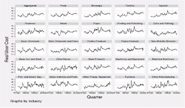
Figures C and C show time-series plots of the capital-output ratio and user costs for each industry in our panel. Note that all three of our primary variables of interest (capital, output and the user cost) vary both in the time and cross-section dimensions. In turn, since corporate tax rates and risk-free rates do not vary across industries, cross-sectional variation in the user cost owes almost entirely to differences across industries in the relative price of capital, anticipated capital gains, and capital depreciation rates.21 In reality, our user cost measure may miss some variations in the user cost stemming from changes in the risk premium, which could vary idiosyncratically over time and across industries and may not be adequately reflected in our measure of borrowing costs. But we think it is quite likely that risk premiums are not integrated processes, so this variation is not an issue--at least asymptotically--in our levels specifications. In the difference specifications, we attempt to limit the influence of potential variations in the risk premium by differencing, and by controlling for fixed and aggregate effects.
5.1 Unit Root Tests
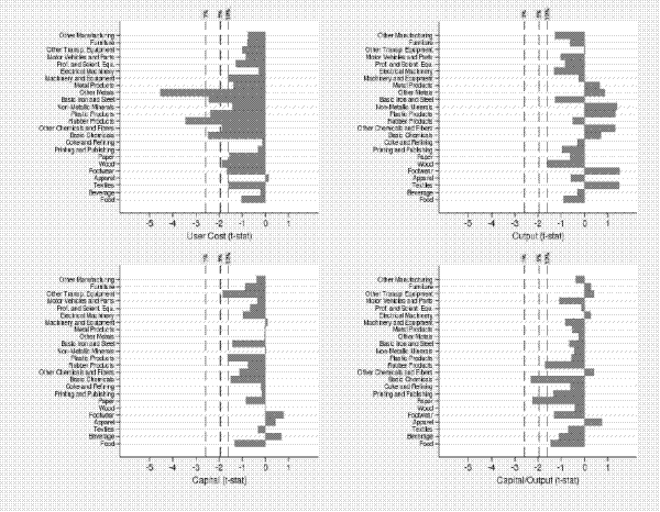
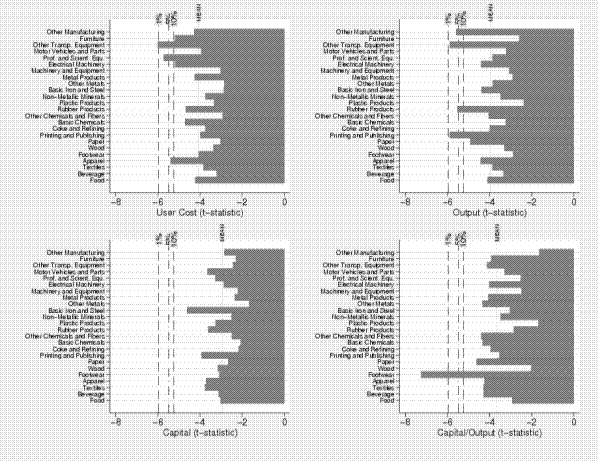
Before proceeding to estimation, we formally test for unit roots in our measures of capital, output, and the user cost. As mentioned earlier, unit roots are necessary to identify frictionless elasticities from long-run responses. We also test for a unit root in the ratio of capital to output, which is a precondition for a cointegrating relation between capital, output, and the user cost. Starting with the single time series tests, Figure C shows the results of Dickey-Fuller GLS tests by industry.22 To correct for small-sample size distortions, we augmented these equations with lag difference terms using the lag selection criterion described in Ng and Perron [2001] to choose an appropriate lag order.23 These tests fail to reject unit roots at 5 percent significance in all but six of the twenty-four industries in our panel. At 10 percent significance, we fail to reject unit roots in all but nine industries.
A potential issue for our analysis is the presence of structural breaks. In our dataset, there is a strong rationale to believe that there may be structural breaks at the time that the embargo was imposed and removed. These structural breaks, if present, could make it difficult to draw inferences about the existence of unit roots, an important characteristic for our estimation. To assess the effect of potential structural breaks, we conduct unit roots tests following the procedure in Clemente, Montañes and Reyes [1998], which is robust for two structural breaks. Figure C shows the results of this test for each industry in our sample. The break-robust tests fail to reject a unit root for capital, output, and the capital-to-output ratio. For the user cost, the tests fails to reject a unit root at 5 percent significance for all but two of the industries in our panel--close to what we would expect from type I error.24
We also tested for the presence of unit roots using panel tests, which have the additional benefit of exploiting information contained in the cross-sectional dimension of the dataset. Table 1 shows the results for a number of alternative specifications. The first
line shows p-values for the panel unit root tests developed by Pesaran [2007], which maintains a null hypothesis that a given variable has a unit root for all industries against the alternative of no unit root in at least one industry.25 The second line of the table shows p-values obtained by applying the Hadri [1999] test to our full dataset, which maintains the
null of stationarity for all 24 industries against the alternative of a unit root. For robustness, we conducted all of these tests both on our full panel of 24 industries and for an "![]() subsample" of industries in which single-series tests failed to reject the presence of a unit root in the user cost at the 10 percent significance level. Taken together, these tests provide support for maintaining that the relevant
variables in our full panel have unit roots at the 5 percent significance level. However, at the 10 percent significance level, the evidence for unit roots in the user cost for all 24 industries in the full panel is mixed. For the
subsample" of industries in which single-series tests failed to reject the presence of a unit root in the user cost at the 10 percent significance level. Taken together, these tests provide support for maintaining that the relevant
variables in our full panel have unit roots at the 5 percent significance level. However, at the 10 percent significance level, the evidence for unit roots in the user cost for all 24 industries in the full panel is mixed. For the ![]() subsample, the panel tests do support the existence of unit roots in the user cost. Since unit roots in the user cost are preconditions for identification, we err on the side of caution by also showing elasticity estimates obtained by restricting
the dataset to just the
subsample, the panel tests do support the existence of unit roots in the user cost. Since unit roots in the user cost are preconditions for identification, we err on the side of caution by also showing elasticity estimates obtained by restricting
the dataset to just the ![]() subsample.
subsample.
5.2 Estimates Using Panel Cointegration Techniques
We begin by estimating a cointegrating specification between capital, output and the user cost. Equation (3) can be rearranged to obtain:
| (6) |
where
![\begin{displaymath} e_{it}=\left[ \begin{array}[c]{ccc}% 1 & -\sigma_{i} & \left( \sigma_{i}-1\right) \end{array}\right] \left[ G(B)-I_{3}\right] \left[ \begin{array}[c]{c}% y_{i,t}\ u_{i,t}\ a_{i,t}^{K}% \end{array}\right] \end{displaymath}](img76.gif)
Small sample bias remains an important econometric issue when testing for cointegration because our sample may not be sufficiently large to overcome finite-sample correlation between the regressors and the structural error term in equation (5.2).28 We estimate our cointegrating relationship using pooled DOLS (Kao and Chiang [2000]) which assumes homogeneity, and mean-group DOLS (Pedroni [2001]) which allows for heterogeneity in the true elasticity across industries. Both of these specifications include dynamic OLS terms that correct for biases that arise in finite samples when there is correlation between the error term and our regressors.29 The structural form of the error in equation (5.2) provides some useful guidance about what variables to include as dynamic correction terms. Specifically, when the conditions for cointegration hold, the error term will generally include lagged differences in both the user cost and output. For this reason, we include first-differenced lags and leads of both of these variables in all of our specifications.30 In addition, we include time dummies and fixed effects in order to correct for biases that arise in the presence of contemporaneous correlation between residuals across industries (Pedroni [2001]).
We begin by testing the validity of the cointegrating relation in equation (5.2) using both our full dataset and the ![]() subsample. We conduct two
sets of tests. The first set is a homogeneous cointegration specification that uses cointegrating residuals from pooled DOLS specifications, while the second set is a heterogenous specification that uses cointegrating residuals fitted using our mean-group DOLS specifications. All of our tests
assess the null hypothesis of no cointegration using test statistics described by Pedroni [1999].31 We conduct these tests for
pooled within-dimension ("panel") statistics that maintain the null that the residuals in all industries have unit roots against the alternative that these residuals have a common stable autoregressive parameter, and for between-dimension ("group") statistics that maintain the null that the cointegrating residuals in all industries have a unit root against the alternative that the residuals in all industries have stable--but not necessarily common--autoregressive
roots.32 The results, shown in Table 2, show that our tests are able reject the null of no cointegration, and provide fairly
strong empirical support for both our homogeneous and heterogeneous cointegrating specifications.
subsample. We conduct two
sets of tests. The first set is a homogeneous cointegration specification that uses cointegrating residuals from pooled DOLS specifications, while the second set is a heterogenous specification that uses cointegrating residuals fitted using our mean-group DOLS specifications. All of our tests
assess the null hypothesis of no cointegration using test statistics described by Pedroni [1999].31 We conduct these tests for
pooled within-dimension ("panel") statistics that maintain the null that the residuals in all industries have unit roots against the alternative that these residuals have a common stable autoregressive parameter, and for between-dimension ("group") statistics that maintain the null that the cointegrating residuals in all industries have a unit root against the alternative that the residuals in all industries have stable--but not necessarily common--autoregressive
roots.32 The results, shown in Table 2, show that our tests are able reject the null of no cointegration, and provide fairly
strong empirical support for both our homogeneous and heterogeneous cointegrating specifications.
Table 3 reports our user elasticity estimates from these two cointegration specifications. The first and second columns of the table report estimates using our full panel of 24 industries and for the ![]() subset of industries, respectively. Results for our pooled DOLS specifications--shown in the top portion of the table--all point to highly significant estimates of the user cost elasticity that are in the neighborhood of the Cobb-Douglas benchmark
of -1.0. All of these pooled specifications include 25 leads and lags of first-differences in output and the user cost, the order of which was determined using a sequential t-test procedure
similar to that described by Ng and Perron [1995].33 This number of dynamic correction terms is in line with specifications used
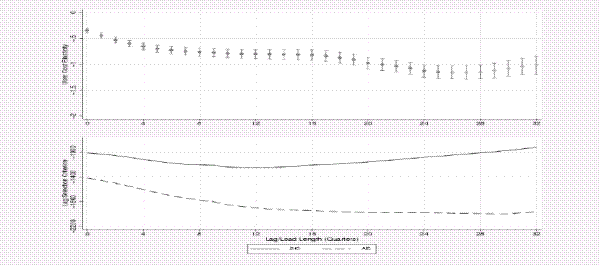
by Caballero [1994] and Schaller [2006] for quarterly equipment capital. Figure C shows how varying the number of included leads and lags affects our estimates. Estimates of the user cost
elasticity--shown in the top panels of the figure--tended to increase in absolute magnitude as we added more dynamic correction terms, but generally remained in the range of -1.0 for a wide
range of possible specifications. The bottom panels of this figure show that our lag/lead length roughly corresponds with what would be suggested by the Akaike Information Criterion.34
subset of industries, respectively. Results for our pooled DOLS specifications--shown in the top portion of the table--all point to highly significant estimates of the user cost elasticity that are in the neighborhood of the Cobb-Douglas benchmark
of -1.0. All of these pooled specifications include 25 leads and lags of first-differences in output and the user cost, the order of which was determined using a sequential t-test procedure
similar to that described by Ng and Perron [1995].33 This number of dynamic correction terms is in line with specifications used
by Caballero [1994] and Schaller [2006] for quarterly equipment capital. Figure C shows how varying the number of included leads and lags affects our estimates. Estimates of the user cost
elasticity--shown in the top panels of the figure--tended to increase in absolute magnitude as we added more dynamic correction terms, but generally remained in the range of -1.0 for a wide
range of possible specifications. The bottom panels of this figure show that our lag/lead length roughly corresponds with what would be suggested by the Akaike Information Criterion.34
The bottom portion of Table 3 summarizes our estimation results using group-mean DOLS. This method estimates separate DOLS specifications for each industry and then forms an estimate of the aggregate elasticity using a weighted average of the industry estimates. To
correct for finite-sample bias, we include in each DOLS regression 8 leads and 16 lags of the first-differences in output and the user cost.35 We find a
user-cost elasticity estimate of -0.54 for the full panel, but the estimate rises in magnitude to -0.85 for the ![]() subsample.
subsample.
In the following section, we present and estimate a distributed-lag specification. The motivation for this alternative specification is two-fold. First, it provides some assurance that our results are robust to alternative econometric specifications. Second, it allows us to test the importance, for estimation, of the exogeneity of shocks to the user cost. We estimate the user cost elasticity during the embargo period and compare it to the elasticity in the non-embargo period. Such an analysis could not be appropriately carried out with the cointegration specification which, under the maintained assumptions, should be consistent even in the presence of such endogeneity.
5.3 Distributed Lag Specification
When shocks to the user cost are exogenous, and both output and the user cost contain unit roots, the first two columns of the matrix ![]() in equation (3) are identical to the first two columns of a three-dimensional identity matrix
in equation (3) are identical to the first two columns of a three-dimensional identity matrix ![]() . Given these assumptions, we can estimate distributed lag
specifications of the form:
. Given these assumptions, we can estimate distributed lag
specifications of the form:
| (7) |
for industries
where the long-run responses are restricted such that
We start by including a large number of lags in our regressions and then apply the sequential t-test procedure described in Ng and Perron [2001] to successively eliminate lags of the user cost that--at the margin--do not contain statistically relevant information about the overall magnitude of the response.38 Figure C shows the results of this lag order selection exercise for two alternative specifications. The circles that denote the estimate at each lag show the outcome of our sequential t-test at that lag: Dark circles denote that the coefficient on the last included lag can be statistically distinguished from zero at 10 percent significance level. The outcome of these sequential t-tests suggest that we include 27 quarterly lags in our baseline specification.39
Table 4 shows estimates from our distributed lag specifications for both the heterogeneity specification that assumes an identical user cost elasticity across industries ("HOM"). We also show results of a seemingly unrelated specification that estimates separate elasticities for each industry, and construct the aggregate elasticity by averaging the industry-specific elasticities ("HET") using as weights each industry's average share of the total nominal capital stock over the sample period.40
The estimated long-run user cost elasticities for these specifications range between -0.48 (heterogeneous specification) and -0.62 (homogeneous specification) for the full sample, both of which are highly significant. For the subsample of industries for which unit root in the user cost is more robust, the estimates of user cost elasticity are larger, ranging from ![]() to -0.83. In the following section, we assess the importance of identification for
estimation of the user cost elasticity by examining the effect of embargo on our estimates.
to -0.83. In the following section, we assess the importance of identification for
estimation of the user cost elasticity by examining the effect of embargo on our estimates.
5.4 Economic Embargo, Endogeneity, and User Cost Elasticity
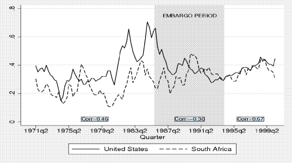
Presumably when the economy became less open during the embargo period (1985-1994), one would expect shocks to the user cost to have become less exogenous because the embargo introduced differences between South Africa's domestic interest rates and the world interest rates, and between domestic and world prices of capital goods. This presumption is borne out in the data. Figure C shows the aggregate user cost for fixed business capital in the United States (a proxy for the world) and for South Africa.41 Though the composition of the business capital stock likely differs in these two countries, broad patterns in these user costs suggest that the cost of capital in South Africa became detached from the rest of the world during the embargo period. The contemporaneous correlation between the two user costs series is highly positive both before and after the embargo, but fell significantly during the embargo. This pattern is consistent with the conjecture that shocks to the user cost during the embargo period were less influenced by exogenous factors.42 In light of this, the identification problem would be heightened during the embargo period, making it more difficult to estimate the user cost elasticity. We formally test this hypothesis by estimating the user elasticity during the embargo and non-embargo periods.
To capture the potential effect on our estimates of this heightened endogeneity, we augment the lagged-difference specification in the preceding section to include terms that interact the observable explanatory variables with a dummy variable for the embargo period. Our formulation for this regression is:
![\begin{displaymath}% \begin{array}[c]{c}% \Delta k_{i,t}=\eta_{i}+T_{t}+N^{y}(B)\Delta y_{i,t}+M^{y}(B)\left( d_{t}\Delta y_{i,t}\right) \\ +N^{u}(B)\Delta u_{i,t}+M^{u}(B)(d_{t}\Delta u_{i,t})+\epsilon_{i,t}\text{,}% \end{array}\end{displaymath}](img100.gif) |
(8) |
so that the embargo affects the entire long run relationship between capital and its fundamentals, but only for observations of capital growth that occur within the embargo period. As in our previous distributed lag specification, we estimate these regressions using contemporaneous observations and 27 lags of each the fundamentals (including the interactions with the embargo dummy). Given these estimates, we determine the long-run elasticity of capital with respect to the user cost by calculating
Results using this specification are shown in Table 5. The first and second columns show estimates using our full panel of 24 industries and the ![]() subsample. We find that the magnitude of the user cost elasticity outside of the embargo period increases from the -0.45 to -0.62 range (in previous section) to -0.75. For the
subsample. We find that the magnitude of the user cost elasticity outside of the embargo period increases from the -0.45 to -0.62 range (in previous section) to -0.75. For the ![]() sample, the estimate increases from the -0.77 to -0.83 range to -0.86. Interestingly, the user cost elasticity for the embargo period is significantly lower and in the -0.25 to -0.27 range, consistent with estimates in many previous studies that document a small and, often, insignificant user cost
elasticity. These results are consistent with the hypothesis that the user cost became more endogenous during the embargo period, leading to a greater role of simultaneity bias. These findings may help explain why studies of the capital-user cost elasticity using stationary specifications and data
from large economies often find very little role for the user cost in determining the size of the capital stock.43 The similarity results from this
specification after correcting for the embargo period to those shown earlier from the cointegration specification is particularly intriguing and suggests that our estimates are fairly robust across econometric specifications.
sample, the estimate increases from the -0.77 to -0.83 range to -0.86. Interestingly, the user cost elasticity for the embargo period is significantly lower and in the -0.25 to -0.27 range, consistent with estimates in many previous studies that document a small and, often, insignificant user cost
elasticity. These results are consistent with the hypothesis that the user cost became more endogenous during the embargo period, leading to a greater role of simultaneity bias. These findings may help explain why studies of the capital-user cost elasticity using stationary specifications and data
from large economies often find very little role for the user cost in determining the size of the capital stock.43 The similarity results from this
specification after correcting for the embargo period to those shown earlier from the cointegration specification is particularly intriguing and suggests that our estimates are fairly robust across econometric specifications.
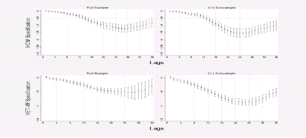
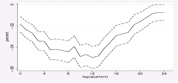
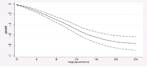
To better describe how capital adjusts to innovations in the user cost, we show the marginal and cumulative responses of capital to a one percent increase in the user cost in figures C and C, respectively. These responses are for our
embargo-corrected estimates using the ![]() subsample-- those for the full sample have similar contours. These marginal responses for our embargo corrected estimates show a distinct hump-shape
that reaches maximum response at about twelve quarters and then gradually attenuates to about zero by the twenty eighths quarter. These responses suggest a rather slow and non-monotonic adjustment process that extends over about seven years. This helps document the importance of focusing on the
long-run in order to capture the full response of the capital stock to effect of a shock to the user cost, and the importance of using a regression specification that is flexible enough to allow the shape of the response to be non-monotonic over time.
subsample-- those for the full sample have similar contours. These marginal responses for our embargo corrected estimates show a distinct hump-shape
that reaches maximum response at about twelve quarters and then gradually attenuates to about zero by the twenty eighths quarter. These responses suggest a rather slow and non-monotonic adjustment process that extends over about seven years. This helps document the importance of focusing on the
long-run in order to capture the full response of the capital stock to effect of a shock to the user cost, and the importance of using a regression specification that is flexible enough to allow the shape of the response to be non-monotonic over time.
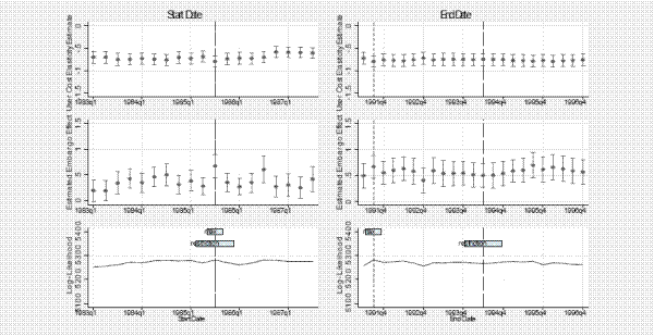
Our estimation assumed that the embargo started in 1985 and ended in early 1994. The exact dating of the embargo period could be uncertain as it is with most event studies. The choice of these dates is supported by anecdotal evidence and narratives on the imposition and removal of the embargo as well as in the aggregate economic data shown earlier. Nonetheless, we conduct sensitivity analyses that vary the embargo's starting and ending dates within a two-year window of our chosen dates. Figure C shows in the bottom panels, the log-likelihood of various starting and ending dates, and the top panels show the corresponding user cost elasticities. The bottom panels show the log-likelihood of each alternative, holding all else equal, while the top and middle panels show corresponding elasticity estimates for the non-embargo and embargo periods, respectively. Our user cost elasticity estimate is not sensitive to reasonable changes in the starting and ending dates of the embargo as shown in the top panels and our starting date (1985) maximizes the log-likelihood.
6 Concluding Remarks
In this study we estimate a statistically significant user cost elasticity between -0.80 and -1.0 which, in most cases, are statistically indistinguishable from the Cobb-Douglas benchmark of -1.0. This study is one of the first to document such a large user cost elasticity for a broad measure of business capital that includes both equipment and structures, and the first to show that similar estimates can be obtained using both stationary and cointegrating regression specifications.
One explanation for our ability to identify a large user cost elasticity is that exogenous shocks to the user cost are better identified in a small and isolated economy like South Africa. In a closed economy or in a large open economy, the capital stock and the user cost of capital are jointly determined by a domestic demand and supply equilibrium that equates the marginal product and marginal opportunity cost of capital services. This simultaneity introduces inconsistency into estimates of the user cost elasticity. In a small open economy like South Africa, however, shocks to the user cost are largely influenced by world interest rates and prices of capital goods that the country takes as given.
The economic embargo that the world imposed on South Africa between about 1985 and early 1994 forced their economy to revert toward autarky. This provides a unique opportunity to determine the extent that endogeneity attenuates estimates of the capital-user cost elasticity. We find a robust correlation between the user cost for South Africa and that of the United States (a proxy for world user costs) before the embargo. This correlation falls significantly during the embargo period, and goes back up after the sanctions are lifted and South Africa is re-integrated into the world economy. We find that during the embargo period, when the user cost became less influenced by exogenous factors, the estimated user cost elasticity fell considerably--to magnitudes that are more in line with those obtained in many previous studies. These results underscore the importance of identification to uncovering the `elusive' user cost elasticity of capital.
A. Appendix: Derivation of Estimation Equation
We start by finding a linearized solution for the firm's capital stock for some arbitrary ![]() for the generalized, linearly homogeneous adjustment cost function
for the generalized, linearly homogeneous adjustment cost function
![]() that satisfies the restrictions described in the main text. After substituting out investment using the capital accumulation constraint in equation (3), the first order condition for the capital stock in this case--after some rearranging--is:
that satisfies the restrictions described in the main text. After substituting out investment using the capital accumulation constraint in equation (3), the first order condition for the capital stock in this case--after some rearranging--is:
![\displaystyle E_{t}\left[ \frac{\partial F(A_{t+1}^{L}L_{t+1},A_{t+1}^{K}K_{t+1})}{\partial K_{t+i}}\right]](img111.gif) |
![\displaystyle =\overline{p}_{t}^{K}\left[ r+\delta-\frac{E_{t}\left[ \Delta p_{t+1}^{K}\right] }{p_{t}^{K}}\right] +](img112.gif) |
(9) |
![\displaystyle {\textstyle\sum\limits_{m=0}^{M}} E_{t}\left[ \overline{p}_{t+m}^{K}\right] (1+r)^{1-m}J_{1+m}(K_{t+1+m}% ,...,K_{t+1+m-M})](img113.gif) |
(10) |
where
![\displaystyle E_{t}\left[ \left( \frac{Y_{t+1}}{K_{t+1}}\right) ^{\frac{1}{\sigma}}% \frac{\left( A_{t+1}^{K}\right) ^{\frac{\sigma-1}{\sigma}}}{U_{t+1}}\right]](img123.gif) |
![\displaystyle =E_{t}\left[ \left( \frac{K_{t+1}^{\ast}}{K_{t+1}}\right) ^{\frac {1}{\sigma}}\right]](img124.gif) |
|
![\displaystyle =1+\frac{% {\textstyle\sum\limits_{m=0}^{M}} \frac{E_{t}\left[ p_{t+m}^{k}\right] }{p_{t}^{K}}(1+r)^{1-m}J_{1+m}% (K_{t+1+m},...,K_{t+1+m-M})}{r+\delta-\frac{E_{t}\left[ \Delta p_{t+1}% ^{k}\right] }{p_{t}^{K}}},](img125.gif) |
where we have used the definition of frictionless capital from (3). Given an assumption
![\displaystyle E_{t}\left[ k_{t+1}^{\ast}\right] \approx k_{t+1}+% {\textstyle\sum\limits_{m=1}^{M}} \overline{d}_{m}\left( k_{t+1+m}-k_{t+1}\right) +% {\textstyle\sum\limits_{m=1}^{M}} d_{m}\left( k_{t+1-m}-k_{t+1}\right) ,](img142.gif) |
(11) |
where
 and and |
||
 for for |
and where
 |
(12) | |
| (13) |
where we have defined the following polynomial in the backshift operator:

| (14) |
Note that this the same general form as the solutions derived by Tinsley [2002] in which firms minimize a quadratic loss objective in which adjustment costs are a function of
At this stage, we let ![]() denote
denote
![]() , so that
, so that
![]() . This factor, which constitutes a moving target toward which capital error-corrects over time, amounts to a weighted average of anticipated future
frictionless stocks where the weights are determined implicitly by the discount factor and the eigenvalues that are embedded in in the lead polynomial
. This factor, which constitutes a moving target toward which capital error-corrects over time, amounts to a weighted average of anticipated future
frictionless stocks where the weights are determined implicitly by the discount factor and the eigenvalues that are embedded in in the lead polynomial
![]() .48 Letting
.48 Letting
![]() denote the
denote the
![]() lead vector
lead vector
![]() , the forward motion of this target can be described by the companion system:
, the forward motion of this target can be described by the companion system:
| (15) | ||
![\displaystyle =a\left( \rho^{-1}\right) E_{t}\left[ {\textstyle\sum\limits_{i=0}^{\infty}} \mathbf{A}^{i}\iota_{M}k_{t+1+i}^{\ast}\right]](img199.gif) |
where
![\displaystyle \mathbf{A}=\left[ \begin{array}[c]{cc}% 0 & I_{M-1}\\ -a_{M}\rho^{-M} & \begin{array}[c]{ccc}% -a_{M-1}\rho^{-(M-1)} & \ldots & -a_{1}\rho^{-1}% \end{array} \end{array} \right] ,](img201.gif) |
(16) |
and
Tevlin and Whelan [2003] show that the forward-looking nature of the capital target is crucial for empirical estimation because the long-run response of capital to an unanticipated change in fundamentals is determined by the degree that this new information affects
the effective capital target ![]() .49 In
turn, this response is closely related to the anticipated persistence of the disturbances. To allow for these expectation effects, we assume that firms forecast the determinants of the frictionless capital stock in equation (3) using the following
VAR(p) process:
.49 In
turn, this response is closely related to the anticipated persistence of the disturbances. To allow for these expectation effects, we assume that firms forecast the determinants of the frictionless capital stock in equation (3) using the following
VAR(p) process:
 , , |
(17) |
where
![\begin{displaymath}\mathbf{C}=\left[ \begin{array}[c]{ccc}% \begin{array}[c]{c}% \begin{array}[c]{c}% C_{1}% \end{array} \\ I_{(p-1)q}% \end{array} & \begin{array}[c]{c}% \begin{array}[c]{c}% \cdots \end{array} \\ \end{array} & \begin{array}[c]{c}% \begin{array}[c]{c}% C_{p}% \end{array} \\ \mathbf{0}_{(p-1)q\times p}% \end{array} \end{array} \right] ,\end{displaymath}](img218.gif)
|
(18) |
is the
After restating the frictionless capital stock in vector form as
![]() , equation (A) can be solved to yield that:
, equation (A) can be solved to yield that:
| (19) |
where we have defined the
![\displaystyle \mathbf{D}\equiv a\left( \rho^{-1}\right) [I_{q}\;\mathbf{0}_{q\times (p-1)q}]% {\textstyle\sum\limits_{i=0}^{\infty}} \left( \iota_{M}^{^{\prime}}\mathbf{A}^{i}\iota_{M}\right) \mathbf{C}^{i+1},](img227.gif) |
(20) |
where
| (21) |
Inserting this representation into equation (A), it can be shown that the optimal capital stock is determined by the equation:
| (22) |
or, after inverting the backshift polynomial
| (23) |
Since
B. Appendix: First Proof
Recall from the previous appendix the definition of the VAR matrix polynomial ![]() shown in equation (A). We begin by showing that if
shown in equation (A). We begin by showing that if
![]() --so that the VAR(p) in equation (A) can be restated as a VAR(p-1) system in
--so that the VAR(p) in equation (A) can be restated as a VAR(p-1) system in
![]() --then
--then
![]() . A necessary condition to establish that
. A necessary condition to establish that
![]() is that all
is that all ![]() of the variables in the VAR(p) contain unit roots.52 Once we establish this result, we turn our attention to cases with
of the variables in the VAR(p) contain unit roots.52 Once we establish this result, we turn our attention to cases with ![]() unit roots, where
unit roots, where
![]() .
.
Begin by defining the matrix
![]() as a
as a
![]() matrix of stacked identity operators
matrix of stacked identity operators
![]() . Using this definition, equation (A), and the fact that
. Using this definition, equation (A), and the fact that ![]() from equation (A), this means that:
from equation (A), this means that:
![\displaystyle G(1)=\mathbf{DS=}a\left( \rho^{-1}\right) [I_{q}\;\mathbf{0}_{q\times q(p-1)}]% {\textstyle\sum\limits_{i=0}^{\infty}} \left( \iota_{M}^{^{\prime}}\mathbf{A}^{i}\iota_{M}\right) \mathbf{C}% ^{i+1}\mathbf{S}](img248.gif) |
(24) |
Straightforward matrix algebra using equation (A) establishes that:
| (25) |
when
![\displaystyle G(1)=a\left( \rho^{-1}\right) [I_{q}\;\mathbf{0}_{q\times(p-1)q}]\mathbf{S}% {\textstyle\sum\limits_{i=0}^{\infty}} \left( \iota_{M}^{^{\prime}}\mathbf{A}^{i}\iota_{M}\right) =I_{q}a\left( \rho^{-1}\right) {\textstyle\sum\limits_{i=0}^{\infty}} \left( \iota_{M}^{^{\prime}}\mathbf{A}^{i}\iota_{M}\right) ,](img253.gif)
|
(26) |
so our desired result boils down to proving that
 |
(27) |
since all the roots of the bottom row companion matrix are stable. Note that the expression on the right hand side of this equation is pre- and postmultiplied by the selection vector
![\begin{displaymath} \left( I_{M}-\mathbf{A}\right) ^{-1}=\left[ \begin{array}[c]{cccccc}% { 1} & { -1} & { 0} & { \cdots} & { 0} & { 0}\ { 0} & { 1} & { -1} & { \cdots} & { 0} & { 0}\ { \vdots} & { \vdots} & { \vdots} & { \ddots} & { \vdots} & { \vdots}\ { 0} & { 0} & { 0} & { \cdots} & { 1} & { -1}\ { a}_{M}{ \rho}^{-M} & { a}_{M-1}{ \rho}^{-(M-1)} & { a}_{M-2}{ \rho}^{-(M-2)} & { \cdots} & { a}% _{2}{ \rho}^{-2} & { 1+a}_{1}{ \rho}^{-1}% \end{array}\right] ^{-1}. \end{displaymath}](img257.gif)
![\displaystyle \equiv\left[ \begin{array}[c]{ccccc}% { 1} & { -1} & { 0} & { \cdots} & { 0}\\ { 0} & { 1} & { -1} & { \cdots} & { 0}\\ { \vdots} & { \vdots} & { \vdots} & { \ddots} & { \vdots}\\ { 0} & { 0} & { 0} & { \cdots} & { 1}% \end{array} \right] _{M-1\times M-1},\qquad N_{2}\equiv\left[ \begin{array}[c]{c}% { 0}\\ { 0}\\ { \vdots}\\ { -1}% \end{array} \right] _{M-1\times1},](img259.gif)
|
||
and
![\begin{displaymath} \left( N_{1}\right) ^{-1}\equiv\left[ \begin{array}[c]{ccccc}% { 1} & { 1} & { \cdots} & { 1} & { 1}\ { 0} & { 1} & { \cdots} & { 1} & { 1}\ { \vdots} & { \vdots} & { \ddots} & { \vdots} & { \vdots}\ { 0} & { 0} & { \cdots} & { 1} & { 1}\ { 0} & { 0} & { \cdots} & { 0} & { 1}% \end{array}\right] , \end{displaymath}](img263.gif)
 Straightforward calculations using this formula show that
We now turn our attention to cases where the VAR(p) in equation A has fewer than ![]() unit roots. Without loss of generality,
assume that the first
unit roots. Without loss of generality,
assume that the first ![]() of the variables in vector
of the variables in vector ![]() have unit
roots. Given this setup, we need to show that the columns of the matrix
have unit
roots. Given this setup, we need to show that the columns of the matrix ![]() that multiply the first
that multiply the first ![]() elements of
elements of ![]() are the same as the first
are the same as the first ![]() columns of the identity matrix
columns of the identity matrix ![]() . As a first step, Appendix B shows that, in the absence of cointegrating relations, the first
. As a first step, Appendix B shows that, in the absence of cointegrating relations, the first ![]() columns of the summed
columns of the summed ![]() polynomial
polynomial ![]() must be the same as the first
must be the same as the first ![]() columns of an identity matrix
columns of an identity matrix ![]() . Now we proceed to calculate
. Now we proceed to calculate ![]() using equation (B). Equation (B) still holds, and the
matrix product
using equation (B). Equation (B) still holds, and the
matrix product
![]() can be decomposed as follows:
can be decomposed as follows:
![\begin{displaymath} \mathbf{CS}=\mathbf{S+}\left[ \begin{array}[c]{c}% C(1)-I_{q}\ \mathbf{0}_{(p-1)q}% \end{array}\right] , \end{displaymath}](img271.gif)
![\begin{displaymath} \mathbf{C}^{i+1}\mathbf{S}=\mathbf{S+}\left[ \begin{array}[c]{c}% H_{i+1}\left( C(1)-I_{q}\right) \ \mathbf{0}_{(p-1)q}% \end{array}\right] , \end{displaymath}](img272.gif)
![\displaystyle G(1)=I_{q}a\left( \rho^{-1}\right) {\textstyle\sum\limits_{i=0}^{\infty}} \left( \iota_{M}^{^{\prime}}\mathbf{A}^{i}\iota_{M}\right) +a\left( \rho^{-1}\right) \left[ {\textstyle\sum\limits_{i=0}^{\infty}} \left( \iota_{M}^{^{\prime}}\mathbf{A}^{i}\iota_{M}\right) H_{i+1}\right] \left( C(1)-I_{q}\right) .](img275.gif)
|
(28) |
Finally, using our results for the
![\displaystyle G(1)=I_{q}+a\left( \rho^{-1}\right) \left[ {\textstyle\sum\limits_{i=0}^{\infty}} \left( \iota_{M}^{^{\prime}}\mathbf{A}^{i}\iota_{M}\right) H_{i+1}\right] \left( C(1)-I_{q}\right) .](img276.gif) |
(29) |
Since the first
C. Appendix: Second Proof
Partitioning the vector ![]() so that the first
so that the first ![]() variables are
variables are
![]() and the remaining
and the remaining ![]() variables are
variables are ![]() . We wish to prove that, when a nonstationary VAR(p) representation of the form shown in equation (A) exists, the first
. We wish to prove that, when a nonstationary VAR(p) representation of the form shown in equation (A) exists, the first ![]() columns of the matrix
columns of the matrix ![]() must be the same as the corresponding columns of the identity matrix
must be the same as the corresponding columns of the identity matrix ![]() .
.
We begin by forming a basis of the space of ![]() vectors
vectors ![]() such that
such that
![]() is
is ![]() . Since the first
. Since the first ![]() elements of
elements of ![]() are assumed to be
are assumed to be ![]() and there are no cointegrating relations linking these variables, one such basis is the
and there are no cointegrating relations linking these variables, one such basis is the
![]() matrix:
matrix:
| (30) |
Therefore, the space of ![]() linear combinations
linear combinations
![]() is spanned by the space of vectors
is spanned by the space of vectors
![]() for any nonzero
for any nonzero ![]() vector
vector ![]() . Since the elements of
. Since the elements of
![]() must be stationary, it can always be written using a Wold representation of the form:
must be stationary, it can always be written using a Wold representation of the form:
| (31) |
and
 where
where
| (32) |
so that any rotation of
Now note that the VAR(p) can be written as
![]() . Premultipling both sides of equation (C) by the expression
. Premultipling both sides of equation (C) by the expression
![]() and simplifying, one obtains the restriction that:
and simplifying, one obtains the restriction that:
| Dataset | User Cost | Output | Capital |
|
||
|---|---|---|---|---|---|---|
| Full Sample | All I(1) | At least one I(0) | 0.093 | 0.485 | 1.000 | 0.924 |
| Full Sample | All I(0) | All I(1) | 0.000 | 0.000 | 0.000 | 0.000 |
| I(1) Subsample | All I(1) | At least one I(0) | 0.363 | 0.101 | 1.000 | 0.903 |
| I(1) Subsample | All I(0) | All I(1) | 0.000 | 0.000 | 0.000 | 0.000 |
Notes: For each sample, the top line reports the p-value for the null hypothesis of a unit root using a version of the CADF panel unit root test devised in Pesaran (2007). In our test, we constructed a "Ztbar" statistic by taking the average of normalized t-statistics across industries, using simulated first and second moments. Asymptotically, this statistic is normally distributed under the null (see Im, Pesaran and Shin [2007]) , a fact that we use to compute the p-value under the null.. Results are not meaningfuly affected when we instead use the critical values in Pesaran[2007]. In an alternative specification, we include a "Trend" to allow for trend-stationary under the alternative hypothesis, doing so does not affect our tests results. These tests are robust for cross-sectional dependence and serial correlation. The number of included lagged differences for each industry was chosen by a sequential t-test criterion in which lags were dropped until that lag was significant at 10 percent for more than 10 percent of the industries. The bottom line for each dataset reports the p-value for the Hadri (1999) panel test, which maintains the null of stationarity. All tests control for fixed and aggregate effects. The Pesaran test is robust for serial correlation and generic forms of cross-sectional error correlation. The results of the Hadri test are robust to serially correlated errors and heteroskedasticity.
Note: Listed p-values are for the null of no cointegration for the statistics described in Pedroni(2001). For the homogeneous specification, residuals are from a cointegrating vector that was fitted using a pooled DOLS specification that included 25 leads and lags of the first-difference of the independent variables. The heterogeneous specifications were estimated using a group-mean DOLS estimator that included 8 leads and 16 lags of the first-differenced independent variables. All estimators control for group fixed effects and and time effects. The results of these tests were unchanged when we restricted the output elasticity to unity.
| Long Run Elasticity of Capital to | Full Panel | I(1) Panel |
|---|---|---|
| HOM: Pooled DOLS User Cost | -0.965 | -1.000 |
| HOM: Pooled DOLS User Cost | (0.064) | (0.072) |
| HOM: Pooled DOLS Sample Size | 1,560 | 975 |
| HET: Group Mean DOLS User Cost | -0.536 | -0.845 |
| HET: Group Mean DOLS User Cost | (0.039) | (0.056) |
| HET: Group Mean DOLS Sample Size | 2,208 | 1,380 |
Note: Pooled DOLS: Specifications include 25 leads and lags of changes in output and the user cost, along with current values. Standard errors are robust for cross-sectional correlation in the error term and autocorrelation. Mean-Group DOLS: Specifications include 8 leads and 16 lags of the first-differences in the user cost and output. Standard errors are robust to cross-sectional correlation and autocorrelation. All specifications control for fixed and aggregate effects.
| Long Run Elasticity of Capital to | Full PanelHOM | Full PanelHET-W | I(1) Panel HOM | I(1) Panel HET-W |
|---|---|---|---|---|
| User Cost ( |
-0.615 | -0.477 | -0.767 | -0.826 |
| User Cost ( |
(0.067) | (0.048) | (0.079) | (0.054) |
| Lags Included | 27 | 19 | 25 | 19 |
| Sample Size |
Note: All regressions include the contemporaneous observation of the dependent variable and lags of the independent variables in addition to industry fixed effects,and aggregate effects. In all specifications, the long-run capital output elasticity is constrained to be one. The estimates denoted "HOM" restrict so that all industries have the same elasticity. The "HET-W" estimates separate user cost elasticities for each industry, then forms an estimate of the aggregate elasticity that weights each industry's estimate by its average share of the total nominal capital stock over the sample period. The number of included lags in each specification was determined using a sequential T test procedure in which the lag length was successively shortened until the coefficient(s) on the last included lag(s) was (were jointly) significant. Standard errors are robust to both cross-sectional correlation and heteroskedasticity in the residuals.
| Long Run Elasticity of Capital to: Period | Full Panel | I(1) Panel |
|---|---|---|
| User Cost: Non-Embargo ( |
-0.749 | -0.858 |
| User Cost: Non-Embargo ( |
(0.074) | (0.085) |
| User Cost: Embargo (
|
-0.250 | -0.265 |
| User Cost: Embargo (
|
(0.108) | (0.134) |
| User Cost: Difference ( |
0.499 | 0.593 |
| User Cost: Difference ( |
(0.115) | (0.142) |
| Lags Included | 27 | 27 |
| Sample Size |
Note: All regressions include the contemporaneous observation of the dependent variable and 27 lags, along with fixed industry fixed effects, and aggregate effects. The number of included lags was determined by performing a sequential T-test procedure for the entire dataset. The robust standard errors account for both cross-sectional correlation and heteroskedasticity in the residuals. All specifications are restricted so that the long-run capital output elasticity is one. Standard errors were calculated using the entire covariance matrix for all estimated parameters.
Figure 1: Ratio of Current Account to Gross Domestic Product for South Africa, 1970 to 2001.
Figure 11: Sensitivity of results from embargo specification to beginning and end dates of the embargo, for speci- fications that are restricted so that the long-run capital-output elasticity is one. Left panels show sensitivity to the begin date, while right panels show sensitivity to the ending date. Top panels: Estimates of corrected user user cost elasticity with 95 percent confidence interval. Middle panels: Estimated effect of embargo on elasticity with 95 percent confidence interval. Bottom panels: Log-likelihood for given start or end date.
Footnotes
![\displaystyle % F(A_{i,t}^{K},A_{i,t}^{L},K_{i,t,},L_{i,t})=\left[ \omega_{i}\left( A_{i,t}^{K}K_{i,t}\right) ^{\frac{\sigma-1}{\sigma}}+(1-\omega_{i})\left( A_{i,t}^{L}L_{i,t}\right) ^{\frac{\sigma-1}{\sigma}}\right] ^{\frac{\sigma }{\sigma-1}}% ,](img12.gif)
![\displaystyle J\left( K_{t+1},...,K_{t+1-M}\right) =K_{t}% {\textstyle\sum\limits_{m=1}^{M}} \tfrac{\theta_{m}}{2}\left[ \left( 1-B\right) ^{m}\left( \tfrac{\Delta K_{t+1}}{K_{t}}\right) \right] ^{2},](img44.gif) |
(4) |
where
 Note that this formula
implicitly assumes that firms expect interest rates, the corporate tax rate, and the rate of depreciation to remain constant in the coming periods-i.e. all tax changes are surprises. Return to Text
Note that this formula
implicitly assumes that firms expect interest rates, the corporate tax rate, and the rate of depreciation to remain constant in the coming periods-i.e. all tax changes are surprises. Return to TextWe also conduct lag order specifications using the Akaike and Schwarz information criteria for each number of included lags. The results did not provide additional useful guidance. Return to Text
![\frac{E_{t}\left[ \Delta p_{t+1}^{k}\right] }{p_{t}^{k}}](img149.gif) drop out in the vicinity of the steady state since
drop out in the vicinity of the steady state since
![\displaystyle % {\displaystyle\sum\limits_{l=1}^{\infty}} \theta^{l}E_{t}\left[ \gamma\left( \Delta k_{t+l}\right) ^{2}+\left( k_{t+l}-k_{t+l}^{\ast}\right) ^{2}\right] .](img172.gif)
![\displaystyle f_{t}=\iota_{M}^{^{\prime}}g_{t}=a\left( \rho^{-1}\right) E_{t}\left[ {\textstyle\sum\limits_{i=0}^{\infty}} \iota_{M}^{^{\prime}}\mathbf{A}^{i}\iota_{M}k_{t+1+i}^{\ast}\right] ,](img179.gif)
