
Federal Home Loan Bank Advances and Commercial Bank Portfolio Composition
Abstract:
The primary mission of the 12 cooperatively owned Federal Home Loan Banks (FHLBs) is to provide their members financial products and services to assist and enhance member housing finance. In this paper, we consider the role of the FHLBs' traditional product - "advances," or collateralized loans to members - in stabilizing commercial bank members' residential mortgage lending activities.
Our theoretical model shows that using membership criteria (such as a minimum of 10 percent of the portfolio being in mortgage-related assets) or using mortgage-related assets as collateral does not ensure that FHLB advances will be put to use for stabilizing members' financing of housing. Indeed, our model demonstrates that advances - a relatively low cost managed liability - are most likely to influence lending only when such liabilities are used to finance "relationship" loans (i.e., loans to bank-dependent borrowers) that will be held on a bank's balance sheet and are least likely to influence lending for loans where the loan rate is heavily influenced by securitization activities, like mortgages.
Using panel vector autoregression (VAR) techniques, we estimate recent dynamic responses of U.S. bank portfolios to FHLB advance shocks, to bank lending shocks, and to macroeconomic shocks. Our empirical findings are consistent with the predictions of our theoretical model. First, recent bank portfolio responses to FHLB advance shocks are of similar magnitude for mortgages, for commercial and industrial loans, and for other real estate loans. This suggests that advances are just as likely to fund other types of bank credit as to fund single-family mortgages. Second, unexpected changes in all types of bank lending are accommodated using FHLB advances. Third, FHLB advances do not appear to reduce variability in bank residential mortgage lending resulting from macroeconomic shocks. However, some banks appear to have used FHLB advances to reduce variability in commercial and industrial lending in response to such macroeconomic shocks. Thus, relatively low cost managed liabilities may be used to finance "relationship" borrowers (which are typically business borrowers, rather than residential mortgage borrowers), although this use for advances appears to have diminished over time.
Keywords: Advances, Government-Sponsored Enterprises, GSE, Portfolio shocks, Panel-VAR
JEL Classification Numbers: G21: Banks, Depository Institutions, Mortgages
G18, G38: Government Policy and Regulation
*The views expressed do not necessarily reflect those of the Board of Governors of the Federal Reserve System, the Federal Reserve Bank of Atlanta, or their respective staffs. We thank Brent Ambrose, Joseph McKenzie, Joe Peek, Larry Wall, and various seminar participants for helpful comments on previous drafts.
1. Introduction
Government-sponsored enterprises (GSEs) represent an unusual intervention by the federal government into private capital markets. GSEs are financial institutions that are individually chartered by Congress, but owned by private shareholders (cooperative members or outside investors depending on
the ownership arrangement). The Congressional charters, extraordinary ongoing interactions between these institutions and government officials, and past government actions have created a perception in financial markets that GSE debt obligations are implicitly guaranteed by the federal government.
This perception allows each institution to borrow at favorable interest rates and then pass some of these savings on to consumers. Hence, by chartering a specific GSE, the federal government can target benefits toward a specific sector of the economy without recognizing the attendant costs in the
federal budget. The three most prominent GSEs are those serving housing: the Federal Home Loan Bank (FHLB) System, the Federal National Mortgage Association (Fannie Mae), and the Federal Home Loan Mortgage Corporation (Freddie Mac).1![]() 2
2
Measuring the extent to which a GSE's primary business activities provide gross social benefits - as defined by its statutory mission - is a critical first step in understanding whether such interventions are desirable. (Of course, even then, one has not accounted for costs, including general equilibrium distortions.) With respect to Fannie Mae and Freddie Mac, a large literature has emerged that attempts to estimate the effect of their activities on mortgage interest rates.3 Remarkably, as noted by McCool (2005), there has been little attempt to examine similar questions for the FHLB System.4 This is the aim of our paper.
The FHLB System is a collection of 12 cooperatively owned wholesale banks. The statutory mission of this GSE is to provide their members financial products and services, including collateralized loans (advances), to assist and enhance such members' financing of (1) housing and (2) community lending.5 Membership is open to all depository institutions with more than 10 percent mortgage assets and also to community financial institutions (i.e., those with less than $587 million in total assets as of December 2005). Over 8,000 financial institutions are currently members of the FHLB System.
In this paper, we focus on the role of FHLB advances in stabilizing commercial bank members' financing of housing.6 We specifically consider three questions. First, are unexpected changes in advances correlated with changes in residential mortgage lending and other forms of bank lending? Second, are unexpected changes in bank loan portfolios, including residential mortgages, accommodated using FHLB advances? Third, do FHLB advances help to insulate bank portfolios from macroeconomic shocks (e.g., unexpected changes in the federal funds rate, the yield curve, or GDP) and do these shocks have less of an effect on residential mortgage lending than on other forms of bank lending?
Toward answering these questions, we first develop a loan pricing model that provides the conditions for relatively cheap, or more steadily priced, FHLB advances to influence loan rates and thereby affect bank credit and, in particular, mortgage credit. As we demonstrate later, if mortgage markets are heavily influenced by securitization or other forms of market-based financing, then a bank might hold a mortgage portfolio (because it "cherry picks" from the flow of mortgage originations) but still have no influence on mortgage pricing or mortgage credit availability.
As suggested by our theory, a better measure of a bank's influence on mortgage markets, relative to other forms of lending, is to compare changes in mortgage supply after either a change in the bank's cost of funds or a change in an exogenous factor that could be offset by a change in a bank's cost of funds. If FHLBs are providing funds that ultimately create more mortgage credit or if they stabilize members' financing of housing -- rather than simply funding all bank assets -- then it is through innovations in supply or demand across loan types that this relationship might be observed.
We use the predictions of the theoretical model to interpret recent dynamic responses of U.S. commercial bank portfolios to FHLB advance shocks, to unexpected loan demand shocks, and to macroeconomic shocks using a panel-VAR. We present the following results. First, bank portfolio responses to FHLB advance shocks are of similar magnitude for mortgages, for commercial and industrial loans, and for other real estate loans. Hence, advances are just as likely to fund other types of bank credit as to fund single-family mortgages. Second, unexpected changes in lending, due to changes in loan demand for example, are accommodated using advances by active FHLB members. Mortgage lending is not unique in this respect. Third, FHLB advances do not appear to have reduced the variability in residential mortgage lending by banks that resulted from either federal funds rate shocks or GDP shocks. However, some banks appear to have used FHLB advances to smooth commercial and industrial lending in response to such macroeconomic shocks, although this use appears to have diminished over time. Therefore, FHLB advances do not appear to be stabilizing commercial bank members' financing of housing. Overall, we find that commercial banks are increasingly relying on FHLB advances as a wholesale funding source and - because money is fungible - advances are being used to fund all types of commercial bank assets, not just residential mortgages.
The rest of the paper is organized as follows: Section 2 provides some background information on the FHLB System to lay the foundation for understanding our theoretical and empirical modeling strategies. Section 3 provides a theory for considering the effects of FHLB advances on bank portfolio lending in the context of modern capital markets. Section 4 describes our empirical approach, while Section 5 discusses our findings. The last section provides a summary.
2. Background: The Federal Home Loan Bank (FHLB) System and FHLB Advances
The FHLB System was created in 1932 and consists of 12 regional wholesale banks (FHLBs) and an Office of Finance that acts as the FHLBs' gateway to the capital markets.7 Each FHLB is a separate legal entity, cooperatively owned by its member financial institutions (commercial banks, thrifts, credit unions, and insurance companies), that has its own management, employees, and board of directors. The individual FHLBs do not generally compete for members as each institution is assigned a distinct geographic area to serve.8 However, the FHLB System is often viewed as a whole because most of the FHLBs' financing takes the form of debt for which the 12 institutions are jointly and severally liable ("consolidated obligations").9 Flannery and Frame (2006) provide a detailed overview of the structure, activities, and risks of the FHLB System.
FHLB System assets totaled just over $1 trillion at year-end 2006.10 Advances comprise the majority of assets ($641 billion, or about 63 percent of total assets). The FHLBs also maintain portfolios of investments ($271 billion on a consolidated basis) and residential mortgage loans purchased from their members ($98 billion on a consolidated basis).11 Around 95 percent of the consolidated asset portfolio of the FHLB System is funded with debt, almost all of which takes the form of the consolidated obligations issued by the Office of Finance. The FHLB System also funds roughly about 5 percent of their assets through equity capital, most of which is derived from mandatory member stock subscriptions.12
Advances are historically the dominant activity conducted by the FHLB System and hence the most natural place to look for an effect of FHLBs on mortgage markets. By law, these collateralized borrowings are to be used only for residential housing finance.13 The most common forms of advance collateral are mortgage-related assets (whole loans and mortgage-backed securities) and U.S. Treasury and Federal Agency securities.14
Beyond the explicit collateral, the FHLBs also have priority over the claims of depositors and almost all other creditors (including depositors and the Federal Deposit Insurance Corporation) in the event of a member's default - known as a "super-lien."15 Importantly, the super-lien may have the effect of muting FHLB incentives to underwrite and price member credit risk.16
Any link between FHLB advance activity and mortgage funding by the GSEs' member financial institutions must be made through the collateral posted on advances. However, this link is likely to have markedly weakened over the past 75 years due to changes in the legal environment, information technology, and financial practice.
During its first 50 years or so of existence, the FHLB System primarily acted as a reliable supplier of long-term funding for thrift industry mortgage lending by making collateralized advances to these depository institutions. During this time, Congress imposed asset limitations on thrifts that resulted in balance sheets almost entirely comprised of residential mortgage-related assets. All depository institutions were also subject to limitations on the interest rates that they paid depositors (under Regulation Q), which periodically resulted in liquidity pinches. Hence, the availability of FHLB advances to thrifts for the purpose of funding mortgages during deposit shortages. Below, we refer to this smoothing of deposit funding for the purpose of originating mortgages as the "mortgage funding view" of FHLB advance activity.17
A series of changes since 1980 significantly altered the U.S. mortgage funding system. First, the Depository Institutions Deregulation and Monetary Control Act of 1980 and the Garn-St. Germain Depository Institutions Act of 1982 terminated the Regulation Q ceiling on savings account interest rates and gave thrifts expanded investment powers. Second, the Financial Institutions Recovery and Reform Act of 1989 opened FHLB membership to all depository institutions with more than 10 percent of their portfolios in residential mortgage-related assets (whole mortgages and mortgage-backed securities). Most recently, the Financial Services Modernization Act of 1999 expanded the mission of the FHLB System to act as a general source of liquidity to "community financial institutions" and lifted the requirement that thrifts be members of this GSE.18
Today, all types of depository institutions are eligible for FHLB membership. Moreover, few depository institutions maintain portfolios heavily concentrated in mortgages, like the thrifts of yesteryear. In addition, mortgage markets are now national in scope because of improvements in information technology, the growth in mortgage securitization, and the related investment in mortgage-backed assets by a wide-variety of domestic and international investors. Hence, any link between FHLB advances and mortgage lending is likely to be much weaker today than in the past. Indeed, given the modest constraint on FHLB membership related to residential mortgage activity, the portfolio composition of most FHLB members (especially the largest members which dominate advance activity), and the simple fact that money is fungible; FHLB advances could be funding virtually any type of asset. Below, we will refer to the view that FHLB advances are but one of many sources of wholesale funds that are not linked to any particular asset type as the "wholesale funding view" of FHLB advance activity.
3. FHLB Advances, Modern Capital Markets, and Bank Lending
This section presents a theoretical model in order to formalize the prior notions about the relationship between FHLB advances and bank lending in general and residential mortgage lending in particular. Our model is based on Heuson, Passmore, and Sparks (2001), who provide a rigorous treatment of the theory as it relates to mortgage markets, as well as Hancock, Lehnert, Passmore and Sherlund (2005), who customized the model for bank capital requirements.
3.1 The Model
Banks, in our model, have a choice between funding their lending on balance sheet using a mix of deposits and FHLB advances or alternatively via securitization. As we described above, the FHLBs are nominally collateralized lenders but because of the super-lien, they can lay claim to all bank assets. This legal right is important because it means that FHLBs, unlike other wholesale liability providers to banks (or equivalently securitizers), do not necessarily need to worry about adverse selection or "cherry picking" of collateral by FHLB members. In other words, the FHLBs may not need a different (and tighter) underwriting standard than the bank itself.
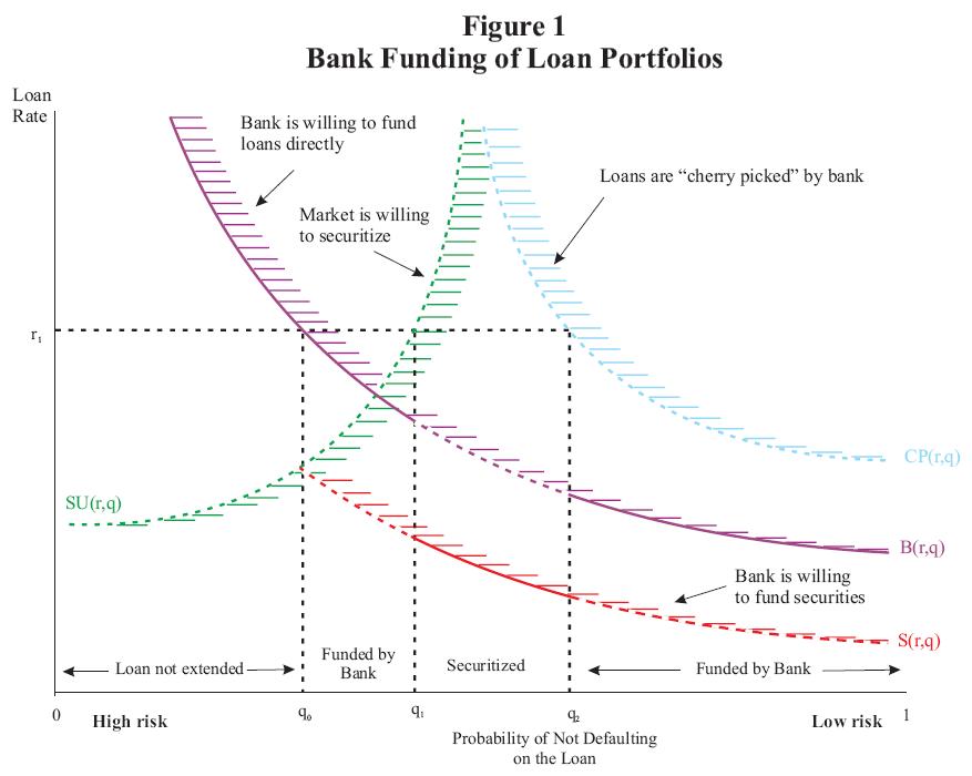
Figure 1 provides a graphical representation of the industry supply curve for a given bank loan market. On the horizontal axis is the probability that borrower will not default, ![]() ,
in a given market segment, which ranges from 0 to 1. Borrowers with higher probabilities of not defaulting (i.e., those closer to 1 in the right corner of the figure) have the lowest credit risks. The marginal cost of bearing borrower credit risks declines as
,
in a given market segment, which ranges from 0 to 1. Borrowers with higher probabilities of not defaulting (i.e., those closer to 1 in the right corner of the figure) have the lowest credit risks. The marginal cost of bearing borrower credit risks declines as ![]() increases, so the lowest rate that a lender is willing to accept falls as the probability of not defaulting on a loan rises.19
increases, so the lowest rate that a lender is willing to accept falls as the probability of not defaulting on a loan rises.19
The purple line (solid and dashed) represents the locus of zero economic profit combinations of loan rates (![]() and credit risks (
and credit risks (![]() from using bank liabilities (including core deposits and FHLB advances) to fund loans directly.20 The bank is
willing to use its liabilities to fund all loans with credit risks equal to, or less than, the credit risks represented by this line (denoted as the set of all points to the right of
from using bank liabilities (including core deposits and FHLB advances) to fund loans directly.20 The bank is
willing to use its liabilities to fund all loans with credit risks equal to, or less than, the credit risks represented by this line (denoted as the set of all points to the right of ![]() .
The red line (solid and dashed) is the locus of zero economic profit combinations of loan rates and credit risks if the bank uses its liabilities to fund securities backed by loans rather than to fund loans directly (denoted
.
The red line (solid and dashed) is the locus of zero economic profit combinations of loan rates and credit risks if the bank uses its liabilities to fund securities backed by loans rather than to fund loans directly (denoted ![]() . Again, the bank is willing to fund all securities with credits risks equal to, or less than, the credit risks represented by this line. Because securities yield a liquidity benefit to the bank, the bank would prefer to use its liabilities to fund
securities, all things equal.
. Again, the bank is willing to fund all securities with credits risks equal to, or less than, the credit risks represented by this line. Because securities yield a liquidity benefit to the bank, the bank would prefer to use its liabilities to fund
securities, all things equal.
However, all things are not equal. Market securities provide a liquidity benefit because they have credit risk properties that can be easily communicated to market investors. Generally, this credit risk is communicated by a high credit rating, a third-party guarantee, and/or a debt structure
that shields investors from credit losses. Market investors also know that banks will tend to keep the best loans and, because only banks can originate loans, they must guard themselves against cherry picking. The loans that a bank will keep are all those with credit risks that are equal to, or
less than, those to the right of the blue dashed line (denoted CP(![]() .
.
Market investors must offset the loan originators' first mover advantage (the "cherry picking") to earn a competitive rate of return, and thus they have a higher credit risk standard than does the bank. This standard is given by the green line -- market investors will only purchase,
securitize, or rate, loans with credit risks equal to, or less than, those represented by the green line (denoted SU(![]() .
.
To summarize, when the loan rate is r![]() , loan originators (which are almost always depositories) only want to sell loans with credit risks between 0 and
, loan originators (which are almost always depositories) only want to sell loans with credit risks between 0 and ![]()
![]() because of cherry picking.21 Moreover, because of this cherry picking activity, market participants only want to use loans with
credit risks between
because of cherry picking.21 Moreover, because of this cherry picking activity, market participants only want to use loans with
credit risks between ![]()
![]() and 1 to create marketable securities. Loans originated by
banks with credit risks lower than
and 1 to create marketable securities. Loans originated by
banks with credit risks lower than ![]()
![]() are placed in the bank's investment
portfolio. Therefore, the effective industry supply curve for loan credit risks of a given product type is represented by the solid segments of the purple and red lines.
are placed in the bank's investment
portfolio. Therefore, the effective industry supply curve for loan credit risks of a given product type is represented by the solid segments of the purple and red lines.
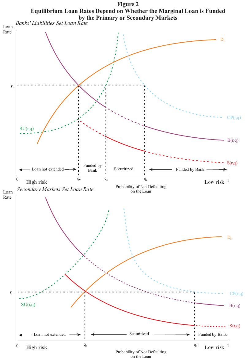
Figure 2 illustrates that equilibrium loan rates are determined by the intersection of supply and demand. The demand curve in this model ranks borrowers by the maximum interest rate they are willing to pay for a loan, suggesting that borrowers with a high probability of paying back their loan are more willing to pay higher interest rates, all other things equal. Loan default is assumed to be costly for borrowers, so that when high interest rates prevail, only borrowers with low odds of default stay in the loan applicant pool.22 This means that the demand curve slopes upward when the probability of not defaulting on a loan is used on the horizontal axis. The equilibrium loan rate for a loan market segment is determined where the demand curve for that segment crosses the industry supply curve.23
3.2 Necessary Conditions for FHLB Advances to Influence Mortgage Interest Rates.
Two necessary conditions must be met in order for FHLB advances to influence mortgage interest rates: (1) the marginal borrower is funded by a bank's liabilities and not by the capital markets, and (2) FHLB advances must be among the bank's lowest cost funding sources. For the mortgage market to respond uniquely, a third condition is also required - that only mortgage loans collateralize FHLB advances and that the banks do not maintain excess collateral.
In the context of the model, FHLBs have the potential to moderate loan rates only if a loan market segment (e.g., mortgage, consumer, commercial and industrial, etc.) demand curve crosses the industry supply curve in the areas where loans, and not securities, are funded by the FHLB member's
liabilities (as shown by the orange line in the top panel of figure 2). Here, the demand curves D![]() crosses the supply curve between q
crosses the supply curve between q![]() and q
and q![]() . Loans to borrowers with credit risks from [
. Loans to borrowers with credit risks from [![]()
![]()
![]()
![]() ] are funded directly with bank liabilities (which include FHLB advances). In contrast, loans to borrowers with credit risks from [
] are funded directly with bank liabilities (which include FHLB advances). In contrast, loans to borrowers with credit risks from [![]()
![]()
![]()
![]() ] are effectively market-priced because the bank swaps the loans for securities at the market rate and then funds the securities by using its liabilities.24 In addition, loans to borrowers who are very good credit risks [
] are effectively market-priced because the bank swaps the loans for securities at the market rate and then funds the securities by using its liabilities.24 In addition, loans to borrowers who are very good credit risks [![]()
![]() 1] are "cherry picked" and held in the bank's investment portfolio and funded with bank liabilities.
1] are "cherry picked" and held in the bank's investment portfolio and funded with bank liabilities.
The bottom panel of figure 2 illustrates an alternative scenario in which the demand curve D![]() cuts across the portion of the industry supply curve where credit risks are borne by the
market. This implies that marginal borrowers are not borrowers with a bank relationship and therefore the bank (and thus FHLB advances) cannot influence loan rates. Instead, loans to borrowers with credit risks from [
cuts across the portion of the industry supply curve where credit risks are borne by the
market. This implies that marginal borrowers are not borrowers with a bank relationship and therefore the bank (and thus FHLB advances) cannot influence loan rates. Instead, loans to borrowers with credit risks from [![]()
![]()
![]()
![]() ] are effectively funded by the market through asset-backed securitization, with the bank's liabilities being used to purchase the securities. Again, loans to borrowers from [
] are effectively funded by the market through asset-backed securitization, with the bank's liabilities being used to purchase the securities. Again, loans to borrowers from [![]()
![]()
![]() 1] are "too good" to
market fund; these loans are funded directly by bank liabilities but only because they yield a competitive return for the bank's investment portfolio.
1] are "too good" to
market fund; these loans are funded directly by bank liabilities but only because they yield a competitive return for the bank's investment portfolio.
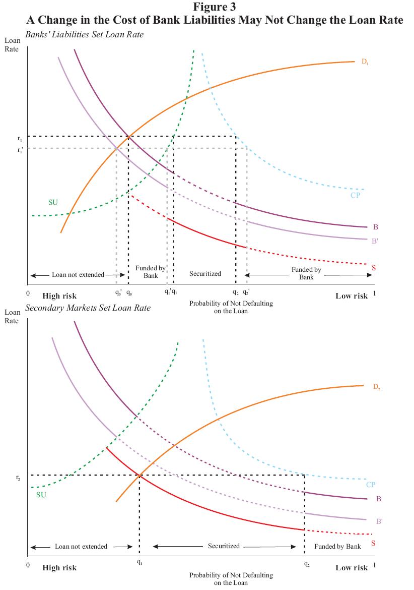
As shown in the top panel of figure 3, which portrays a loan market where borrowers are funded on the margin by bank liabilities, rates on FHLB advances can potentially influence loan rates. However, in order for this to occur, FHLB advances must be among a bank's lower cost funding
alternatives, so as to lower the bank's cost of funds (shown by the move from curve B to curve B![]() in figure 3). This lower cost of funds would cause loan rates to fall because the bank
provides funds to the marginal borrower in the loan market (and banking markets are assumed to be competitive). In other words, the FHLB advance must actually be a lower cost of funds than other wholesale liability alternatives.
in figure 3). This lower cost of funds would cause loan rates to fall because the bank
provides funds to the marginal borrower in the loan market (and banking markets are assumed to be competitive). In other words, the FHLB advance must actually be a lower cost of funds than other wholesale liability alternatives.
The bottom panel of figure 3 alternatively portrays a loan market where the bank's borrowers are funded on the margin by market-priced funding. In this case, lowering the bank's own cost of funds does not influence loan rates. Thus, when securitization plays an important role in a loan market, a lower cost for FHLB advances would be unlikely to influence loan rates. Because mortgage lending is especially influenced by securitization in practice, and because most banks have substantial excess potential collateral, FHLB advances seem unlikely to influence mortgage rates and mortgage lending. However, this is ultimately an empirical question to which we will now turn.
4. Estimation of Bank Portfolio Dynamics
This section describes data and the specification we use to estimate the dynamic interactions between the various components of banks' balance sheets and aggregate economic conditions.
4.1 FHLB Advances Data
Information on FHLB advances held by FHLB members (ADV) is available on a quarterly basis from the Federal Housing Finance Board.25 Table 1 provides data on advances outstanding and FHLB capital stock ownership as of 2006:Q3 for thrifts and commercial banks stratified into three asset size groups (less than $100 million, $100 million to $1 billion, and greater than $1 billion). Strikingly, commercial bank borrowers greatly out number - more than four to one - thrift borrowers (column (2)). Indeed, about half of FHLB advances outstanding are to commercial bank members (columns (3) and (4)), which also own almost half of the FHLB System's capital stock (column (5)). And these advances are concentrated in the largest entities: Commercial banks with greater than $1 billion in total assets, institutions that have many sources of wholesale funding, hold more than one-third of FHLB advances outstanding (column (4)). Below, we focus our study on commercial banks given their increasing importance to the FHLB System and because these lenders have greater opportunity to employ advances for many different types of loans -- not only for residential mortgages.
Because asset-liability management is typically centralized within a banking organization, we constructed asset and liability data at the "top holder" level. For example, a bank holding company, which is comprised of a lead bank and several subsidiary banks, would be the top holder of the banking organization. We aggregated individual bank asset and liability information to the domestic top holder level using information from the National Information Center (NIC), which is the central repository containing information about all U.S. banking organizations and their domestic and foreign affiliates. A bank that is unaffiliated with any other bank is considered to be its own top holder organization.
Bank top holder entities were stratified into three size groups in each quarter: (1) Small top holders have total assets at or below the 50th percentile of the distribution of total assets; (2) medium top holders have total assets between the 50th and 95th percentiles of the distribution of total assets; and (3) large top holders have total assets at or above the 95th percentile of the distribution of total assets. These percentile cutoffs for the three top holder size groups allocate top holders such that 43 percent of the sample is considered "small", 51 percent of the sample is "medium", and 6 percent of the sample is "large" as of 2006:Q3 (table 2). These top holder percentage allocations across the three size groups roughly correspond to those for commercial banks in table 1: small banks (less than $100 million in assets), 38 percent; medium banks ($100 million to $1 billion in total assets), 55 percent; and, large commercial banks (greater than $1 billion in total assets), 7 percent.
As of quarter-end 2006:Q3, only 66 percent of the smallest top holder members borrowed from a FHLB and together they borrowed just $6.4 billion (table 2). In contrast, about 83 (92) percent of medium (large) top holders borrowed from their FHLB and together these entities borrowed $56..1 billion ($304.5 billion). Thus, actual FHLB borrowings are heavily skewed towards the largest top holder banking organizations.
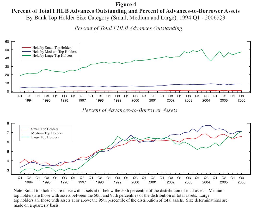
Figure 4 presents quarterly time-series information on the percent of total FHLB advances outstanding and on the percent of advances-to-borrower assets for each of three top holder size groups for 1994:Q1 through 2006:Q3, inclusive. Over this period, large top holder FHLB members, who have many sources of wholesale funding, have steadily increased their share of total FHLB advances outstanding (top panel) as the proportion of their assets funded by FHLB advances has risen and kept pace with advance usage by smaller top holders (bottom panel).
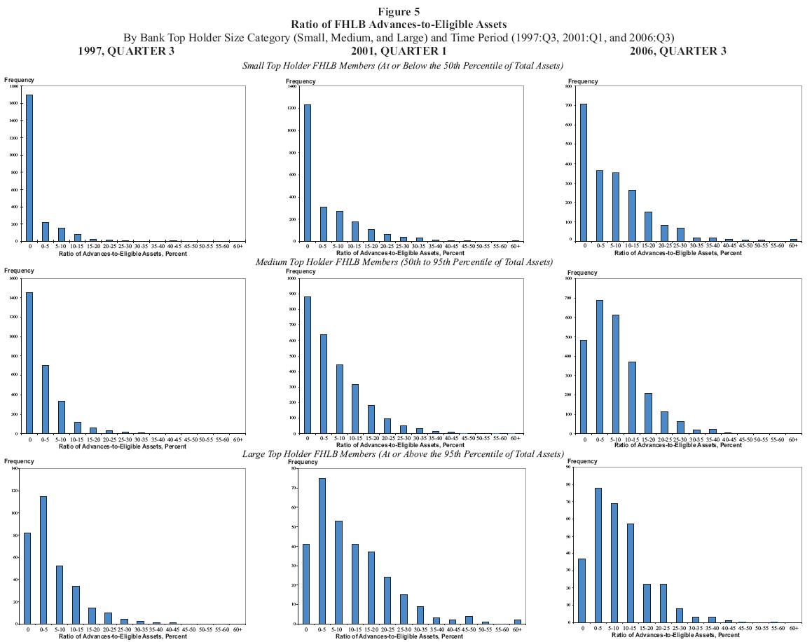
FHLB System members generally have a stock of eligible advance collateral that far exceeds their actual advance borrowings. Figure 5 presents histograms for advances-to-eligible asset ratios (in percent) for small top holders (top panel), medium top holders (middle panel), and large top holders (bottom panel) at quarters-end, 1997:Q3 (left panel), 2001:Q1 (middle panel) and 2006:Q3 (right panel).26 Looking across the top and middle panels of Figure 5, it is clear that a fairly high proportion of small- and medium-sized top holder FHLB members respectively had no advances at all. This pattern did not hold true for the large top holder FHLB members (bottom panel). Regardless of top holder size, virtually all top holder FHLB members used much less than 50 percent of their eligible collateral for FHLB advances, suggesting that collateral is not a binding constraint for commercial banks.
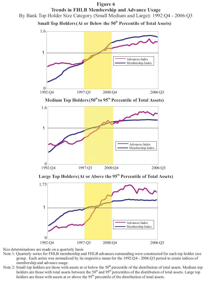
Figure 6 presents aggregate time-series information on the number of FHLB members and their advances outstanding for the three top holder size groups during 1994:Q1 through 2006:Q3. Each series was normalized by its respective time-series mean during the sample period so changes in growth can more easily be discerned.
Interestingly, there appear to be three distinct time periods for the growth rates of FHLB membership and advance usage. During the first period (1994:Q1 - 1997:Q2), membership grew rapidly, but advance usage grew only modestly. This difference in growth patterns across the two indices suggests that new FHLB members were not actively using FHLB advances to fund their asset portfolios during this first period. Consequently, we do not use data from this first period to consider the dynamic interactions between bank balance sheets and aggregate economic conditions. In contrast, during the second period (1997:Q3 - 2000:Q4), which is shaded in figure 6, advance usage grew at least as rapidly as did FHLB membership. In addition, advance usage growth was most rapid for the largest top holders. This difference in growth patterns is consistent with FHLB members (new and old alike) more actively using FHLB advances to fund their portfolios. Because this is likely a learning period for banks not familiar with using FHLB advances, we consider data from this period separately from the later period (2001:Q1-2006:Q3) when FHLB membership is stable and FHLB advance usage appears to be responding to other factors. Indeed, we consider this later period the most useful for understanding whether FHLB advances are influencing mortgage rates or stabilizing members' financing of housing.
4.2 Bank Portfolio Data
Call Reports for individual, federally-insured, domestically chartered commercial banks were used to construct quarterly data for five balance sheet components - residential mortgages (MORT), other real estate loans (OREL), securities (SEC), commercial and industrial loans (C&I), and domestic deposits (DEP).27 Call Reports generally include book values, rather than market values, for each balance sheet component.28
Data were constructed for four asset categories. When feasible, only domestic loans were included in each of these asset categories. Residential mortgages (MORT) include (1) the amount of all permanent loans secured by first liens on 1-to-4 family residential properties, (2) the amount of all
permanent loans secured by junior (i.e., other than first) liens on 1-to-4 family residential properties, and (3) the amount outstanding of "home equity lines."29![]() 30 Other real
estate loans (OREL) consist of (1) construction and land development loans, (2) loans secured by farmland, (3) loans secured by multi-family (5 or more unit) residential properties, and (4) loans secured by nonfarm nonresidential properties.31 Securities (SEC) equaled the sum of the amortized cost for "held-to-maturity" securities and fair value for "available-for-sale" securities.32 Lastly, the amount of commercial and industrial loans (C&I) includes loans to borrowers domiciled in both the U.S. and abroad.33
30 Other real
estate loans (OREL) consist of (1) construction and land development loans, (2) loans secured by farmland, (3) loans secured by multi-family (5 or more unit) residential properties, and (4) loans secured by nonfarm nonresidential properties.31 Securities (SEC) equaled the sum of the amortized cost for "held-to-maturity" securities and fair value for "available-for-sale" securities.32 Lastly, the amount of commercial and industrial loans (C&I) includes loans to borrowers domiciled in both the U.S. and abroad.33
In addition, data were constructed for domestic deposits (DEP). These deposits include transaction accounts, non-transaction savings deposits, and total time deposits less than $100,000.34
4.3 Time-Series Information Concerning Commercial Bank Portfolios
For each top holder size group, quarterly aggregate portfolio share data were constructed for entities without advances and for two types of FHLB members. 35![]() 36 The "active FHLB members" had a ratio of FHLB advances-to-total assets greater than or equal to 2.5 percent. In contrast, "passive FHLB members" had a ratio of FHLB advances that was both greater than zero and less than 2.5
percent. Both top holder size groups and FHLB advance usage status were determined on a quarter-by-quarter basis.
36 The "active FHLB members" had a ratio of FHLB advances-to-total assets greater than or equal to 2.5 percent. In contrast, "passive FHLB members" had a ratio of FHLB advances that was both greater than zero and less than 2.5
percent. Both top holder size groups and FHLB advance usage status were determined on a quarter-by-quarter basis.
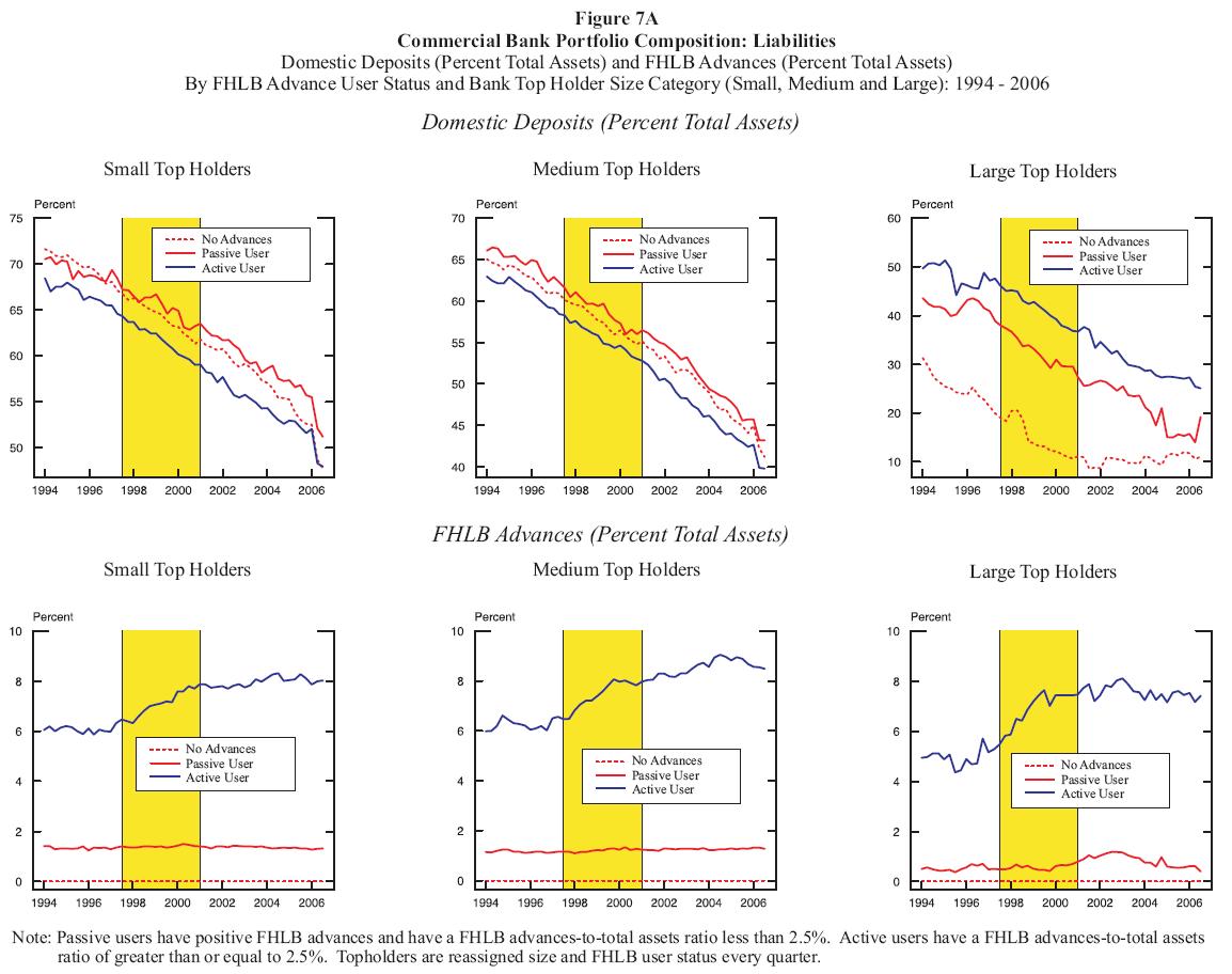
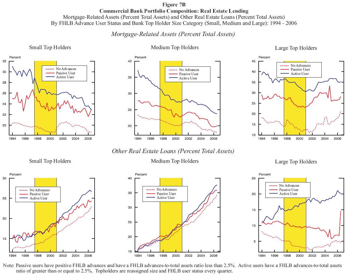
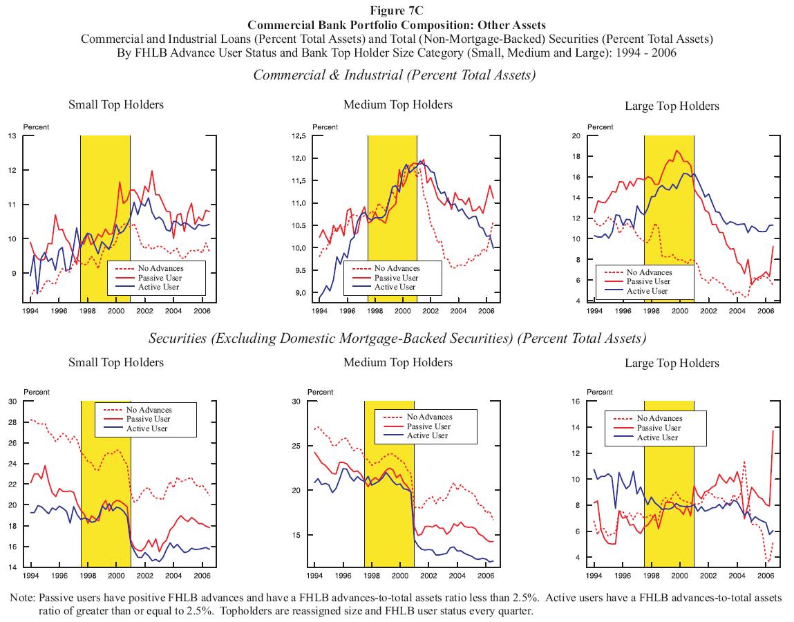
The time-series information on portfolio composition for the top holders stratified by asset size and by FHLB advance usage status is presented in figure 7. Panel A contains time-series on two liabilities: domestic deposits and FHLB advances. Panel B contains time-series on two types of real estate asset categories: mortgage-related assets, which consist of mortgages and mortgage-backed securities, and other real estate (OREL) loans. Panel C contains time-series on commercial and industrial (C&I) loans and on securities, excluding mortgage-backed securities. In each of these three panels, aggregate time-series for small top holders is presented on the left, aggregate time-series for medium top holders is presented in the middle, and aggregate time-series for large top holders is presented on the right. (Note that shading is used in each panel to distinguish the three distinct periods that were described above for FHLB membership and advance usage where only the second period (1997:Q3 - 2000:Q4) is shaded.)
Focusing on the liability side of the portfolio (panel A), the domestic deposit portfolio shares for small top holders and for medium top holders were quite similar for active FHLB members, passive FHLB members, and entities that did not use advances by the end of the period (2006:Q3). This pattern, however, did not emerge for the largest top holders. The large active FHLB member top holders continued to rely more heavily on domestic deposits than did other large top holders. By construction, active FHLB members had a higher proportion of their total assets funded by FHLB advances than did passive FHLB members (panel A, bottom).
Turning to real estate lending (panel B), active FHLB members held higher proportions of their total assets in mortgage-related assets than did passive FHLB members, regardless of their top holder size. Moreover, passive FHLB members held a higher proportion of their assets in mortgage-related assets than did entities without advances, regardless of their top holder size. These patterns are not surprising given that most FHLB members have at least 10 percent of their portfolio in mortgages due to FHLB membership requirements. Moreover, as suggested by the theory presented above, entities that specialize in mortgage origination may hold a higher proportion of their portfolio in mortgages even if they have no influence on mortgage pricing or mortgage credit availability because they can "cherry pick" the highest quality mortgages along the credit risk continuum.
Interestingly, the time-series patterns for the portfolio shares of other real estate lending (panel B, bottom) were quite different across the three top holder size groups: Over the period, small top holder FHLB members increased their other real estate portfolio share modestly, medium top holder FHLB members increased their other real estate portfolio share rapidly, and large top holder FHLB members, who had the smallest such portfolio share at the beginning of the period, had a modest increase in their other real estate portfolio. Small top holder FHLB members with advances held similar proportions of other real estate loans in each quarter regardless of whether they were active or passive members. This similarity in the time-series data across active and passive FHLB members for other real estate loan portfolio shares was also apparent for medium top holder FHLB members. In contrast, large top holder active members held substantially higher proportions of other real estate loans in their portfolios than was held by large top holder passive members.
The time-series for commercial and industrial (C&I) lending portfolio shares (panel C, top) indicate that small- and medium-sized top holder FHLB members with advances did not have as dramatic of a run-off in their commercial and industrial portfolio after the turn of the century as did entities without advances. For the largest top holders, active FHLB advance users appear to have been able to mitigate the run-off in the commercial and industrial lending portfolio whereas passive FHLB advance users had a steep decline in this lending activity. Nevertheless, the passive FHLB advance users among the largest top holders held about the same proportion of their portfolio in commercial and industrial loans as did small- and medium-sized top holders by the end of the sample period.
Small- and medium-sized top holders that did not rely on FHLB advances tended to hold a higher proportion of their portfolio in securities excluding mortgage-backed assets (and a correspondingly lower proportion of their portfolio in the three lending categories (i.e., mortgage-related assets, other real estate loans, and commercial real estate loans)) than did comparably-sized FHLB members (panel C, bottom). Since these top holders did not employ FHLB advances, this higher portfolio share for securities excluding mortgage-backed assets may have been held either for liquidity purposes or to meet (unexpected) increases in loan demands. In contrast, the largest top holders without FHLB advances held similar proportions of securities (excluding mortgage-backed assets) as did comparably-sized FHLB advance users. Unlike other top holders, the largest top holders would have been more likely able to tap managed liability markets to meet their liquidity needs or to fund unexpected increases in loan demands.37 Alternatively, the high proportions of securities in the portfolio for small- and medium-sized top holders may have resulted from fairly modest lending opportunities relative to the availability of domestic deposit funding for these entities.
It is also informative to compare the liability structures of top holders with advances to the top holders without advances for each top holder size group (table 3).38 The liability structures are quite similar for small and medium top holders once one controls for FHLB advance usage, but large top holders have a different liability structure: Large top holders fund a higher proportion of their assets with managed liabilities, subordinated debt, and other liabilities than do smaller top holders. Focusing on the highlighted rows, small and medium top holders with advances tend to fund a slightly higher proportion of their assets with advances than do large top holders with advances. For the small and medium top holder size categories, top holders without advances funded a greater proportion of their assets with equity capital and with core deposits than did top holders with advances. In contrast, for the largest top holder size category, those with FHLB advances funded a greater proportion of their assets with core deposits than did those without advances.
4.4 Macroeconomic Conditions Data
Several data series were constructed at a quarterly frequency to gauge aggregate economic conditions. Our measure of aggregate output - quarterly gross domestic product (GDP) - is measured in real time (i.e., without any subsequent revisions).
These data were obtained from the Federal Reserve Bank of Philadelphia. Our measure of the short-term interest rate - the quarter-end daily federal funds rate (FFR) - was collected from the Federal Reserve Economic Database (FRED) maintained by the Federal Reserve Bank of St. Louis. Our measure of
the slope of the yield curve - the difference between quarter-end 10-year and 1-year Treasury rates (YIELD) - was computed using constant maturity Treasury yields, which are also available from the FRED.39
4.5 Econometric Model
There is considerable evidence that banks typically make portfolio-wide but gradual, adjustments to their holdings of both financial assets and liabilities in response to unexpected events. For example, using aggregate data, Bernanke and Blinder (1992) and Den Haan, Sumner, and Yamashiro (2004) estimate that interest rate shocks affect the size and composition of banks' portfolios for more than two years. Analogously, Hancock and Wilcox (1995) use individual bank data to estimate that portfolio adjustments can take two to three years to complete after a bank capital shock. There are several explanations for why bank portfolio adjustments are gradual and have differing speeds across balance sheet categories, including: the complexity of loan documentation, the difficulty of judging the quality of loan applicants, the speed with which loan applicants alter their loan demand in response to changing circumstances, and the relative liquidity of secondary markets for the different portfolio components.
We use a panel-VAR technique to obtain banks' dynamic responses to portfolio and macroeconomic shocks because of the ability of this type of model to approximate complicated, interdependent adjustment paths with fairly short time-series information. Our first-order nine-equation VAR system takes
into account the dynamic effects on individual banks of unexpected changes in their own balance sheets (i.e., residential mortgage loans (MORT), other real estate loans (OREL), commercial and industrial loans (C&I), deposits (DEP), securities, (SEC), and advances (ADV) and of the relatively
more exogenous economic conditions (the short rate measured by FFR, YIELD measured by the difference between the 10-year Treasury rate and the 1-year Treasury rate, and GDP). We also allow for individual heterogeneity in the levels of the variables by introducing fixed effects, ![]()
![]() . In notational terms, our panel-VAR model is:
. In notational terms, our panel-VAR model is:
The six bank balance sheet variables are measured in logs. A log specification ameliorates the error-term heteroskedasticity that un-logged variables would almost certainly entail. It also has a significant advantage over a portfolio shares specification because it permits a bank's size to change in response to shocks. In contrast, the aggregate economic condition variables - GDP, FFR, and YIELD - are measured in levels with output in nominal dollars and interest rates in percent.
Impulse-response functions, which are reported below, are based on VARs with variables in the flowing order: (1) FFR, (2) YIELD, (3) GDP, (4) MORT, (5) C&I, (6) OREL, (7) DEP,
(8) SEC, and (9) ADV.41 This order is ranked from the most exogenous to the most endogenous of the variables. Therefore, when one considers the
impulse-response function matrix, the federal funds rate, FFR, does not respond to any of the other variable in the system in the first (i.e., contemporaneous) period, but FHLB advances, ADV, respond to everything in that period. In our theory, advances are extended in response to the demands of
profit-maximizing banks; these banks base their decision on the price of advances relative to other funding choices and on the availability of advances based on whether advances are uniquely suited to mortgage lending. This suggests that advances should be treated as the most endogenous of the
variables in the VAR model, relative to macroeconomic variables (which are the most exogenous to the bank) and relative to forms of lending (which are simultaneously determined conditional on the cost of funding).42
Within this model structure, we can test the response of advances to unexpected changes in all types of lending. As suggested by our theory, if advances are uniquely suited for mortgage funding and are critical for funding the borrower on the margin, then advances should not rapidly respond to shocks to other forms of lending (i.e., the "mortgage funding view.") But if advances are just one of many sources of wholesale funding or do not influence the marginal borrower, then the response of advances to, say, an unexpected increase in mortgage loan demand, should be similar to an unexpected increase in demand for other types of loans (i.e., the "wholesale funding" view.)
These distinctions can be illustrated in figure 2, where the demand curve moves upward and to the left. As shown in the top panel, a profit-maximizing bank would demand more advances in response to a positive loan shock. If advances were uniquely suited to mortgages, then only a mortgage loan shock would generate this response. However, as shown in the bottom panel, a loan shock does not influence a bank's demand for funds if securitization funds the borrower on the margin. Thus, if we order the VAR so that advances are influenced quickly by unexpected loan shocks, but can only influence loans themselves with a lag, we can examine both the uniqueness of mortgage funding in generating advance demand and the responsiveness of advances to various loan shocks. In order words, as articulated in our theory, this ordering is consistent with the demand for funding by a profit-maximizing bank.
Along similar lines, if advances have a role in encouraging mortgage funding, then our variable ordering is also consistent with our theory. If the FHLBs put advances on "sale," the shift in a bank's cost of funds (as illustrated in the top panel of figure 3) would influence loan demand when advances played a significant role in a bank's cost of funds, assuming the bank was key in funding marginal borrowers in that loan market (the contrast between the top and bottom panels of figure 3). Using our VAR model, and assuming that FHLB pricing influences the cost of funds with some delay, we can examine how responsive loan demand is to lower prices for FHLB advances.
Finally, using the structured VAR proposed above, we can examine whether or not FHLB advances help to smooth the response of member mortgage lending to unexpected macroeconomic fluctuations (such fluctuations, according to our theory, could be mitigated if advance pricing was adjusted to offset
unexpected loan demands in either mortgage or other forms of lending, assuming advances were important in funding the marginal borrower). If the smoothing role is unique to mortgage funding, it would be readily apparent in a VAR model with this structure, when applied to both banking organizations
with and without FHLB advances. 43
- Empirical Results
We consider impulse responses that trace out the response of current and future values of top holders' portfolio components (e.g., mortgages, C&I loans, and other real estate loans) to a one-standard deviation increase in the current value of various VAR errors, assuming that each error returns to zero in subsequent periods and that all other errors are equal to zero. More specifically, we consider top holders' responses to one-standard deviation shocks to (1) FHLB advances, (2) three lending categories (mortgages, C&I loans, and other real estate loans) and (3) two measures of macroeconomic conditions (federal funds rate and GDP). We consider each in turn.
5.1 Bank Loan Responses to Advance Shocks: Are Mortgages Different?
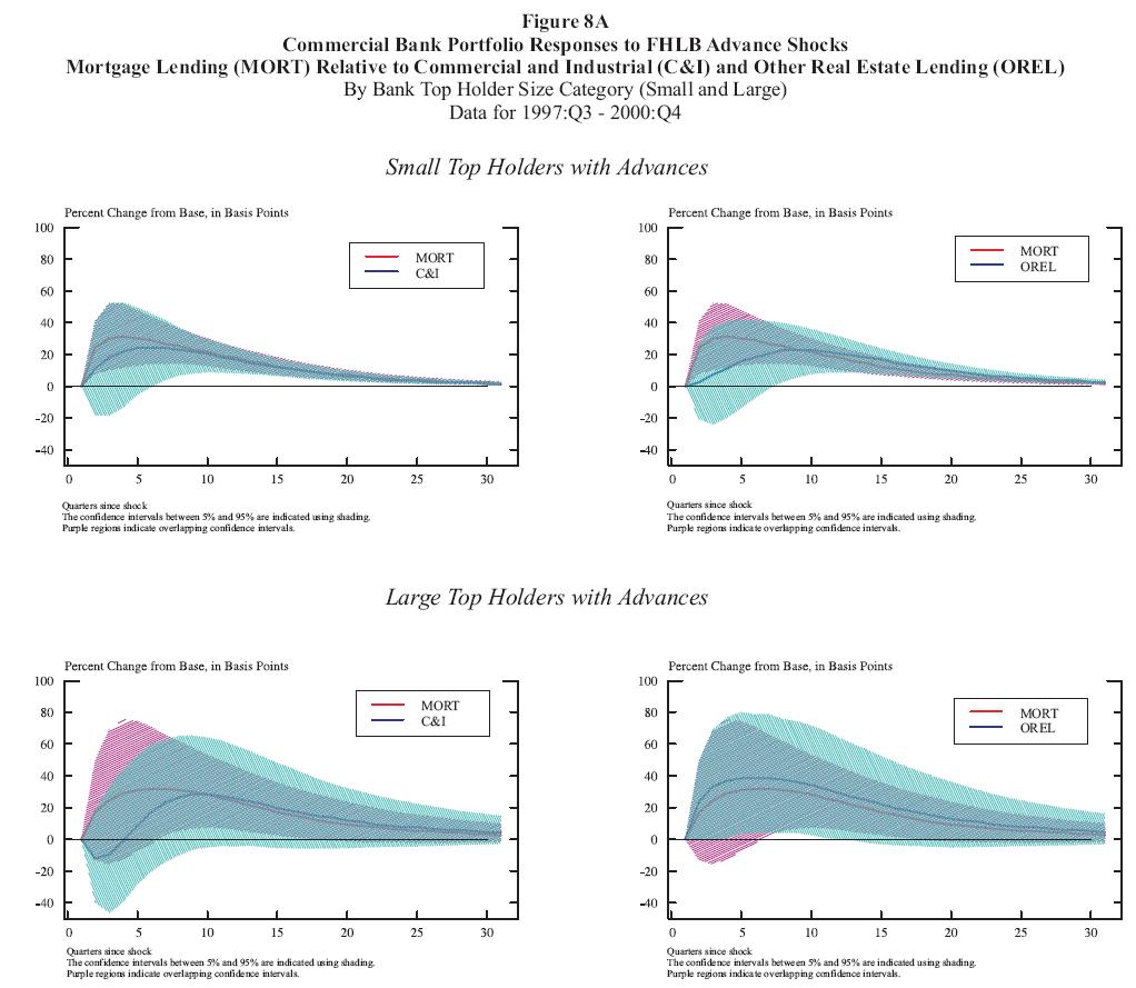
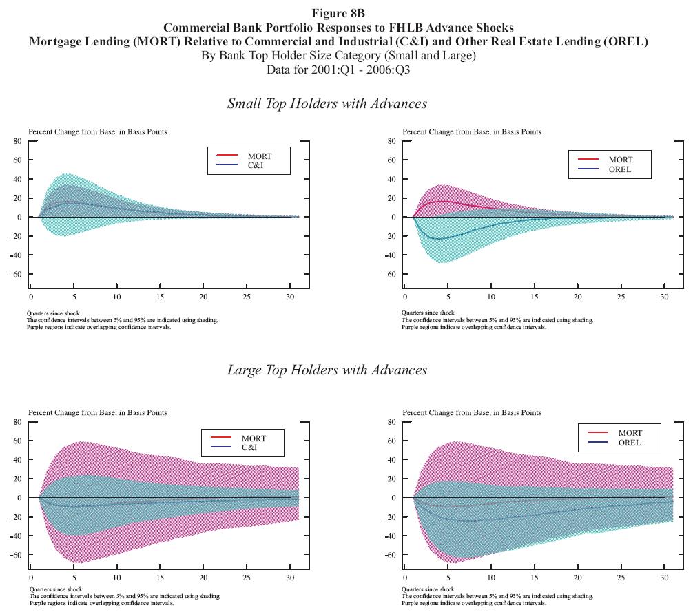
Figure 8 presents impulse-response functions of mortgages (MORT), commercial and industrial (C&I) loans, and other real estate loans (OREL) for a standardized one-standard deviation shock to FHLB advances for small top holder members (top panel) and for large top holder members (bottom panel) for the first period (panel A) and second period (panel B), respectively.44
The top panels show that small top holder members have a statistically significant positive mortgage loan response to a one standard deviation FHLB advance shock in both periods. The shaded regions indicate the 5 percent and 95 percent confidence intervals. The confidence intervals are above zero for the small top holder member mortgage response in each period, though the lower bound of the shaded region is barely above zero in the latest period. This is not the case in both periods for either the C&I or OREL loan responses for these small top holder members, which are not statistically different from zero.
Notably, the positive and significant small top holder member mortgage responses are within the confidence intervals for the small top holder member C&I responses (OREL responses) provided in the top left (right) panel of figures 8A and 8B. Thus, a one standard-deviation advance shock has statistically similar effects on mortgages, on C&I loans, and on other real estate loans for these member groups, suggesting that mortgages are not unique in their response to a shock in FHLB advances. (Portfolio responses of medium top holder members -- not shown -- to a one-standard deviation advance shock had similar patterns to those shown for small top holder members.)
The bottom panels of figures 8A and 8B show that large top holder members do not significantly change their mortgage, C&I, or other real estate lending in response to a one-standard deviation FHLB advance shock. Also, as was the case for small top holder members, an advance shock has statistically similar effects on mortgages, on C&I loans, and on other real estate loans for large top holder members.
Overall, the confidence intervals for C&I lending responses and for mortgage lending responses overlap one another for the advance shocks in both periods. This suggests that advance shocks change C&I and mortgage lending in a similar fashion.
5.2 FHLB Advances Response to Bank Loan Shocks
Bank loan shocks, perhaps due to an increase in the demand for loans of a specific type, could potentially be accommodated by FHLB members using advances. To ascertain whether FHLB members employ advances in this manner, we consider how (unexpected) changes in lending affected FHLB advance usage.
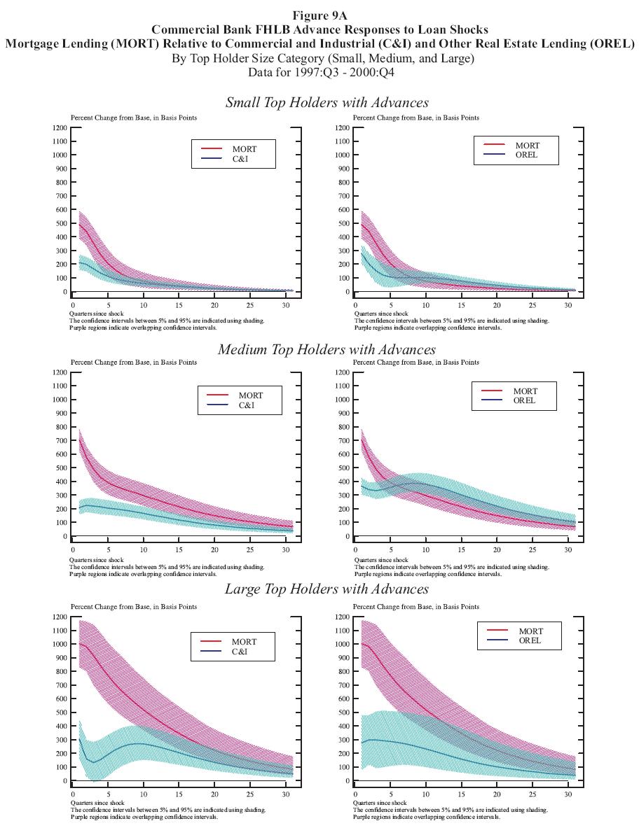
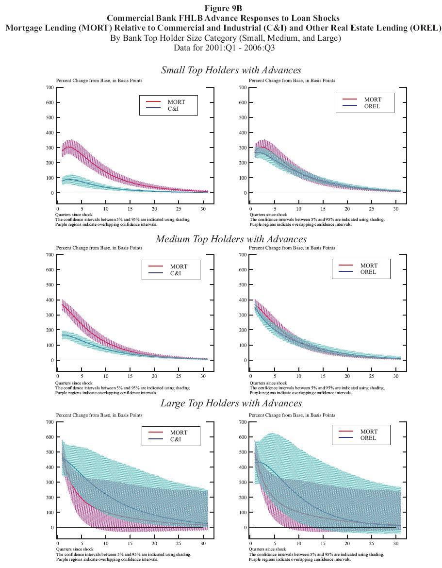
Figures 9A and 9B present for the first and second periods respectively impulse-responses of FHLB advances (ADV) for standardized one-standard deviation shocks to mortgage (MORT) loans, to commercial and industrial (C&I) loans, and to other real estate loans (OREL) for small top holder members (top panel), medium top holder members (middle panel), and large top holder members (bottom panel). On the left side of each figure A and B, the response of advances to a mortgage loan shock is compared to the response of advances to a C&I loan shock. And on the right side of each figure A and B, the response of advances to a mortgage loan shock is compared to the response of advances to a shock in other real estate loans (OREL).
Interestingly, during both periods, the estimated response of current and future values of FHLB advances to a positive (standardized) one-standard deviation mortgage loan shock results in the current value of advances rising; the percent change from the base is positive and statistically significantly different from zero based on the 5 percent and 95 percent confidence intervals for small, medium, and large top holders with advances. Moreover, the estimated percent change from the base for the current value is larger as one peruses down the figure from small to large top holders with advances.
Comparing the magnitudes of the advance responses to mortgage shocks with the advance responses to C&I shocks (left side, figures 9A and 9B), it is apparent that the advance responses are smaller for C&I shocks than for mortgage shocks for both small- and medium-sized top holders with advances in both the first and second periods. This is not the case for the large top holders with advances. Such entities have estimated advance responses that are of statistically similar magnitudes for a C&I shock and for a mortgage shock in the second period.
In the first period, the responses of advances to mortgage shocks is larger than the responses of advances to other real estate lending shocks for top holders with advances regardless of size group (right side, figure 9A). This statistically larger response, however, is short-lived lasting about one-year for small- and medium-sized top holders and about two-years for large top holders.
By the second period, however, the distinction between the responses of advances to mortgage shocks and to other real estate lending shocks is not material (right side, figure 9B). Strikingly, the 5 percent and 95 percent confidence bands for these impulse-response functions for FHLB advances are intertwined. Although the responses of advances to a mortgage loan shock or to an other real estate loan shock are each (positive and) statistically significant, the confidence intervals together indicate that neither response of advances is significantly different from the other.
Overall, the positive and statistically significant estimated responses of FHLB advances to shocks in all three lending categories considered for both estimation periods suggests that FHLB members of all sizes (with advances already) do use this funding source to accommodate unanticipated changes in various types of lending - not only to accommodate unanticipated changes in mortgage lending.
5.3 Portfolio Responses to Macroeconomic Shocks: The Role of FHLB Advances
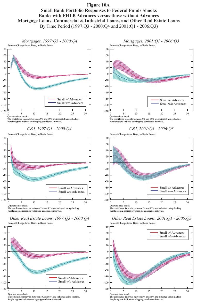
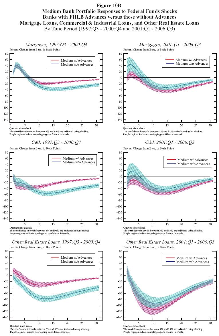
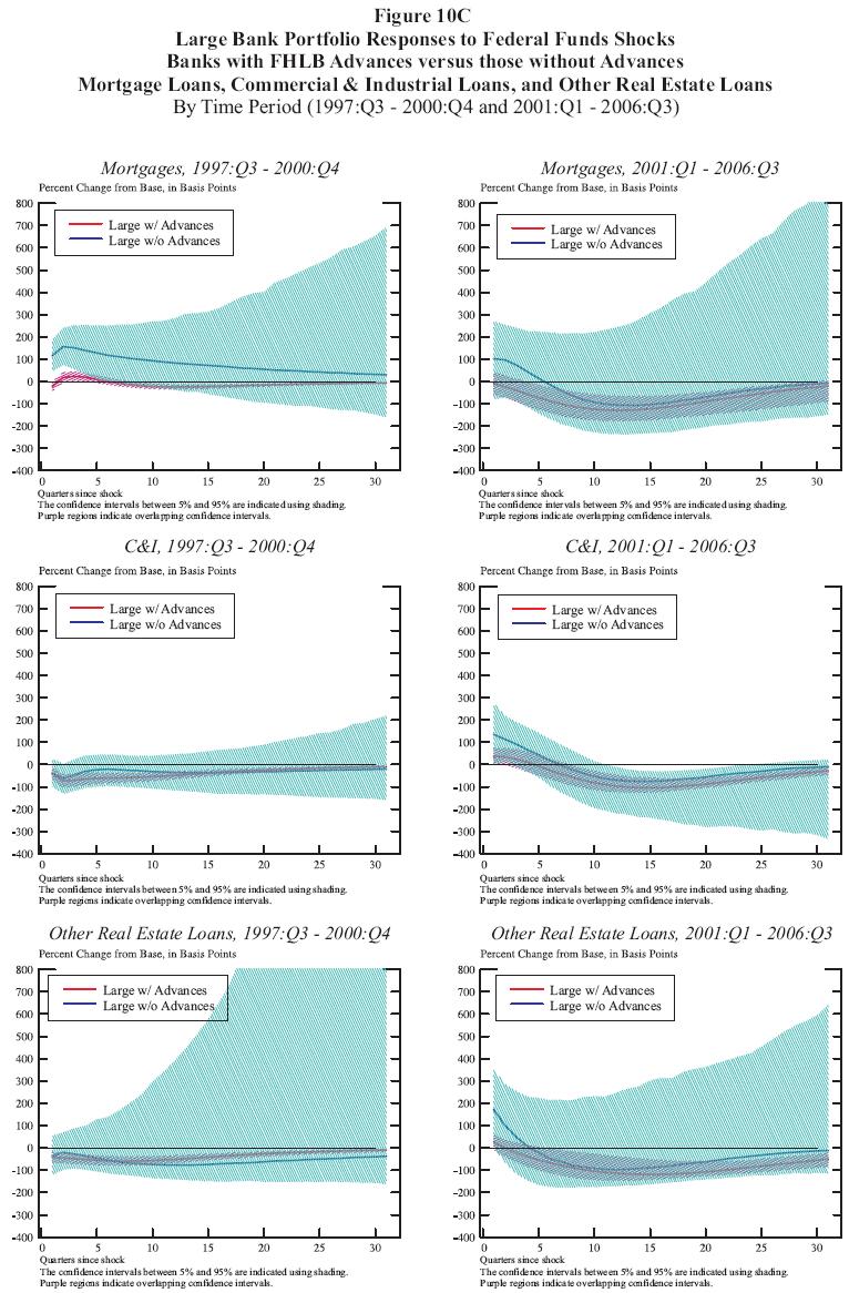
Federal Funds Shocks. For the first period (left side) and for the second period (right side), the estimated responses (with the shaded 5 percent and 95 percent confidence intervals) of mortgages (top panel), of commercial and industrial loans (middle panel) and of other real estate loans (bottom panel) to a federal funds shock are presented in figure 10 for small top holders (panel A), medium top holders (panel B) and large top holders (panel C).45 In each panel of figure 10, the responses of top holders with advances (for a size class) are compared to the responses of top holders (both members and non-members) without advances (for the same size class). These responses are measured using the percent change from the base value for the portfolio category type.
First, consider the portfolio responses of small top holders to a one-standard deviation federal funds shock during the first period (left side, panel A). Regardless of the loan category, the response to a one standard-deviation federal funds rate increase was statistically less negative for small top holders with advances than the corresponding response for small top holders without advances. Therefore, in the first period, the estimated responses for the loan portfolio are consistent with small top holder FHLB members using FHLB advances to reduce the impact of a (positive) federal funds rate shock on their loan customers.
Turning to the second period, an unexpected one standard-deviation federal funds increase (0.29 percent) resulted in a significantly more positive response in mortgage lending by small top holders with advances than by small top holders without advances (top right side, panel A). In fact, the initial increase in mortgage lending for small top holders without advances was not significantly different from zero and within a year of the federal funds shock this response became significantly negative. With respect to commercial and industrial lending and other real estate lending, the estimated responses to a one-standard deviation federal funds shock were not statistically different from one another for small top holders with and without advances. That is, the 5 percent and 95 percent confidence bands for the impulse-response function of small top holders with advances overlays the 5 percent and 95 percent confidence bands for the response of the respective loan type of small top holders without advances. These findings are consistent with a federal funds rate shock having the same effect on the non-mortgage lending portfolios of small top holders with and without advances in the second period.
The responses of medium top holder lending portfolios (figure 10, panel B) to a one-standard deviation federal funds rate shock are quite similar to the responses of small top holder lending portfolios to such a shock. In the first period, the estimated responses for the loan portfolio are consistent with medium top holder FHLB members using FHLB advances to reduce the long-term (negative) impact of a (positive) federal funds rate shock on their loan customers. But in the second period, the estimated portfolio lending responses to a federal funds rate shock are statistically indistinguishable across medium top holders with and without advances.
The portfolio lending responses of large top holders to a federal funds shock are presented in panel C. Because there are so few large top holders without advances, the 5 percent and 95 percent confidence bands around each of the estimated portfolio lending responses are quite wide for this group. As a result, the portfolio responses of large top holders with and without FHLB advances to a federal funds shock are generally statistically indistinguishable.46 Nevertheless, the estimated impulse-response functions for mortgages in the first period are statistically less positive during the first four quarters after a one-standard deviation federal funds shock for the large top holders with advances than for the large top holders without advances. The smaller magnitude of the response by large top holders with advances is not consistent with FHLB members stabilizing housing finance by using FHLB advances, but it may be the case that large top holders without advances lend to mortgage customers that are less sensitive to interest rate shocks than are the mortgage customers that borrow from large top holders with advances.
Overall, our findings suggest that recent portfolio lending responses to a federal funds shock are similar for top holders with and without FHLB advances. The smaller (negative) mortgage, commercial and industrial, and other real estate lending responses to a one-standard deviation federal funds shock for small- and medium-sized top holders with FHLB advances than for small- and medium-sized top holders without advances during the 1997:Q3- 2000:Q4 period suggests that small-and medium-sized FHLB members who use advances employed them to dampen the effects of interest rate shocks on their loan customers including their "bank-dependent" borrowers.
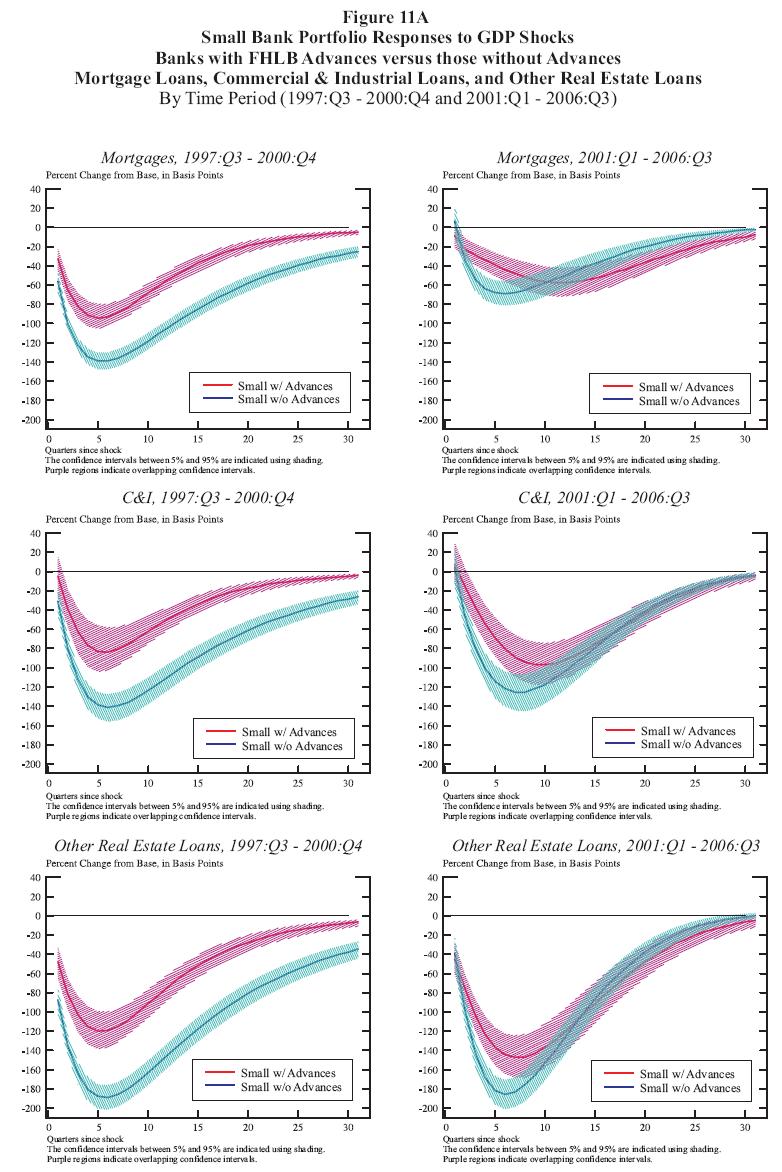
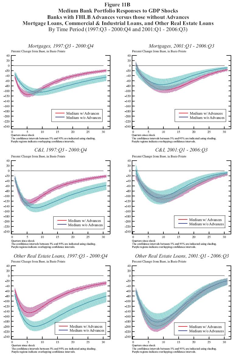
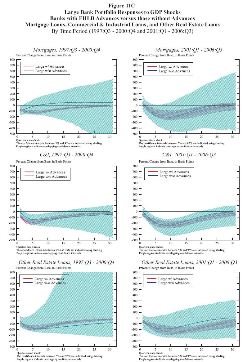
GDP Shocks. Estimated responses of mortgages (top panel), commercial and industrial loans (middle panel) and other real estate loans (bottom panel) to a (standardized) one-standard deviation gross domestic product shock are presented in figure 11. This figure has the same layout as figure 10, so responses for the first period (1997:Q3-200:Q4) are presented on the left side and responses for the second period (2001:Q1-2006:Q3) are presented on the right side with panels A, B, and C corresponding to small-, medium-, and large-sized top holders, respectively. Each estimated portfolio response for each top holder size group is measured using the percent change from its respective base.
Panel A of figure 11 presents the estimated portfolio responses to a negative gross domestic product (GDP) shock for small top holders with and without advances. Looking across the three lending types (mortgage, commercial and industrial, and other real estate lending) in each period considered, there is a dampened (negative) response to a GDP shock of small top holders with advances (red solid line) compared to the mortgage response to a GDP shock of small top holders without advances (blue solid line). Moreover, this different response is statistically significant since the shaded confidence intervals for lending responses of small top holders with advances (red shaded area) are not always intertwined with the confidence interval for lending responses of small top holders without advances (blue shaded area). Particularly for the first period, the impulse-response functions (and their associated confidence intervals) are consistent with FHLB members using advances not only to stabilize mortgage lending, but also to smooth fluctuations in their lending to bank-dependent borrowers.
In panel B, the portfolio responses of medium top holders to a one-standard deviation GDP shock are presented. Focusing on the first period (left panel), the estimated longer-term (more than four quarter out) medium top holder responses to a (negative) GDP shock are less negative for medium top holders with advances (red line) than for medium top holders without advances (blue line) for all three lending types - mortgages, commercial and industrial loans, and other real estate loans. Moreover, the non-overlapping confidence intervals that correspond to these estimated responses imply that these responses tended to be statistically different from one another. These findings are consistent with the wholesale funding view that money is fungible. In the second period, regardless of the lending type, the confidence intervals around the impulse-response functions are intertwined for medium top holders with and without advances. In this later period, the portfolio responses to a GDP shock for medium top holders with advances are statistically indistinguishable from the responses to a GDP shock for medium top holders without advances. These results are consistent with advances not playing a special role with regard to stabilizing mortgage lending over the business cycle.
As was the case with the confidence bands around the portfolio responses to a federal funds rate shock, the confidence bands around the portfolio responses to a GDP shock are wide for large top holders without advances (panel C). There are simply not enough degrees of freedom to concisely estimate such responses since most large top holders are FHLB members.47 Regardless, the estimated impulse-response functions for each of the three lending types presented are quite similar for large top holders with and without advances. Moreover, none of the three portfolio responses to a GDP shock for large top holders with advances are statistically different from the respective portfolio responses to a GDP shock for large top holders without advances. These findings are consistent with the portfolio responses to GDP shocks of large top holders with advances being the same as the portfolio responses to GDP shocks of large top holders without advances. Interestingly, the statistically indistinguishable responses of commercial and industrial lending to a one-standard deviation GDP shock for large top holders with and without advances is consistent with the view that these lenders tend to make loans to less bank-dependent borrowers (i.e., borrowers with more collateral or higher net worth) than smaller top holders who are more likely to specialize in relationship-based loans (e.g., Frame, Srinivasan, and Woosley 2001; Berger 2003).
6. Summary of Findings and Conclusion
In principle, a relatively low cost for FHLB advances does not guarantee that loan rates for borrowers will be lower. Moreover, using membership criteria (such as a minimum of 10 percent of the portfolio being in mortgage-related assets) or using mortgage-related assets as primary collateral does not ensure that FHLB advances will be put to use for stabilizing members' financing of housing. Indeed, our theoretical model shows that subsidized funding is most likely to be used for "relationship" loans (i.e., loans to bank-dependent borrowers) that will be held on a bank's balance sheet and are least likely to be used for loans where the loan rate is heavily influenced by securitization activities. Thus, it is an empirical question whether FHLB advances result in mortgage credit being more available or result in more stable mortgage credit markets.
Using a panel VAR approach, we estimate commercial bank top holders' responses to unexpected FHLB advances, to unanticipated changes in their portfolio, and to shocks in macroeconomic conditions. With regard to shocks to FHLB advances, confidence intervals for C&I lending responses and for mortgage lending responses overlapped one another in both periods considered. This implies that advance shocks change C&I and mortgage lending in a similar fashion.
Loan shocks, perhaps due to an increase in demand for loans of a specific type, appear to be accommodated by FHLB members by using advances, regardless of the loan type. A one-standard deviation (positive) loan shock (for mortgages, for commercial and industrial loans, or for other real estate loans) resulted in (positive) statistically significant changes in FHLB advances in both periods considered, regardless of the top holder size group. Interestingly, advance responses were larger for mortgages than for C&I lending and other real estate lending for all top holder size groups in the 1997-2000 period, but these differences were generally not material in the 2001-2006 period. These findings suggest that FHLB advances are used to accommodate changes in the demand for all types of loans across bank's portfolios. That is, our findings support the view that FHLB advances are like other forms of non-deposit bank funding and will be put to use to increase the overall return for a banking organization.
With respect to macroeconomic shocks (i.e., federal funds rate shocks and GDP shocks), smaller institutions with advances have smaller (negative) responses than do smaller institutions without advances. This is true for both mortgage and C&I lending. These findings are consistent with smaller institutions using FHLB advances for their bank dependent (relationship-based) borrowers. Across time, there has been a diminished difference in responses to macroeconomic shocks across smaller institutions with and without advances. This finding is consistent with smaller institutions having a wider availability of wholesale funding options more recently. In contrast, large top holders with and without advances had similar responses of their loan portfolio to such macroeconomic shocks. This finding is consistent with the view that these lenders tend to make loans to less bank-dependent borrowers (i.e., borrowers with more collateral or higher net worth) than smaller top holders who are more likely to specialize in relationship-based loans
Overall, our findings are consistent with the view that FHLB advances are not special, but rather are a general source of liquidity. The bulk of the empirical evidence suggests that FHLB advances are not connected to mortgage funding in the sense of uniquely funding mortgages or stabilizing mortgage funding. In other words, FHLB advances are fungible.
| Entity Type | Number of Entities | Number of Borrowers | Advances Outstanding (Billions) | % of FHLB Advances | % of FHLB Capital Stock | % of Advances to Borrower Assets |
|---|---|---|---|---|---|---|
| Asset Size | (1) | (2) | (3) | (4) | (5) | (6) |
| Commercial Banks: Less than 100 million | 2,260 | 1,457 | 5.9 | 0.9 | 1.2 | 6.7 |
| Commercial Banks: 100 million to 1 billion | 3,239 | 2,594 | 52.0 | 8.1 | 9.7 | 6.7 |
| Commercial Banks: Greater than 1 billion | 441 | 393 | 227.9 | 35.4 | 33.3 | 6.0 |
| Commercial Banks: Subtotal | 5,940 | 4,444 | 285.8 | 44.4 | 44.1 | -- |
| Thrifts: Less than 100 million | 380 | 232 | 1.5 | 0.2 | 0.4 | 11.3 |
| Thrifts: 100 million to 1 billion | 734 | 622 | 30.1 | 4.7 | 4.7 | 13.9 |
| Thrifts: Greater than 1 billion | 152 | 142 | 296.5 | 46.0 | 39.6 | 18.4 |
| Thrifts: Subtotal | 1,266 | 996 | 328.2 | 51.0 | 44.7 | -- |
| Bank Top Holder Size Category | Number of Top Holders | Number of Borrowers | Borrowers (Percent of Top Holders) | Advances Outstanding (Billions) | Percent of FHLB Advances | Percent of Advances to Borrower Assets |
|---|---|---|---|---|---|---|
| column number | (1) | (2) | (3) | (4) | (5) | (6) |
| Small | 2166 | 1419 | 65.5 | $6.4 | 1.0 | 6.6 |
| Medium | 2584 | 2133 | 82.5 | $56.1 | 8.7 | 7.1 |
| Large | 297 | 274 | 92.3 | $304.5 | 47.3 | 7.1 |
| Total | 5047 | 3826 | 75.8 | $367.0 | 57.0 | -- |
| Memo: 10 Largest Top Holder Members | 10 | 10 | 100.0 | $134.8 | 20.9 | 6.9 |
| TOP HOLDER SIZE Balance Sheet Items | Year-end 2001, Top Holders With Advances (Billions of Dollars) | Year-end 2001, Top Holders With Advances (Percent of Total Assets) | Year-end 2001, Top Holders Without Advances (Billions of Dollars) | Year-end 2001, Top Holders Without Advances (Percent of Total Assets) | Year-end 2005, Top Holders With Advances (Billions of Dollars) | Year-end 2005, Top Holders With Advances (Percent of Total Assets) | Year-end 2005, Top Holders With Advances (Billions of Dollars) | Year-end 2005, Top Holders With Advances (Percent of Total Assets) |
|---|---|---|---|---|---|---|---|---|
| Small: Total Liabilities: Core Deposits | 41 | 70 | 69 | 74 | 62 | 67 | 65 | 72 |
| Small: Total Liabilities: Foreign Deposits | 0 | 0 | 0 | 0 | 0 | 0 | 0 | 0 |
| Small: Total Liabilities: Subordinated Debt | 0 | 0 | 0 | 0 | 0 | 0 | 0 | 0 |
| Small: Total Liabilities: Large Time Deposits | 7 | 13 | 12 | 13 | 13 | 14 | 13 | 14 |
| Small: Total Liabilities: Other Managed Liabilities | 4 | 7 | 1 | 1 | 7 | 8 | 1 | 1 |
| Small: Total Liabilities: FHLB Advances | 4 | 6 | 0 | 0 | 6 | 6 | 0 | 0 |
| Small: Total Liabilities: Other | 0 | 1 | 1 | 1 | 1 | 1 | 1 | 1 |
| Small: Total Equity Capital | 6 | 10 | 11 | 12 | 9 | 10 | 12 | 13 |
| Small: Total Assets | 59 | 100 | 93 | 100 | 92 | 100 | 91 | 100 |
| Medium: Total Liabilities: Core Deposits | 342 | 68 | 152 | 72 | 490 | 65 | 134 | 69 |
| Medium: Total Liabilities: Foreign Deposits | 1 | 0 | 1 | 0 | 1 | 0 | 0 | 0 |
| Medium: Total Liabilities: Subordinated Debt | 0 | 0 | 0 | 0 | 0 | 0 | 0 | 0 |
| Medium: Total Liabilities: Large Time Deposits | 68 | 13 | 30 | 14 | 121 | 16 | 32 | 17 |
| Medium: Total Liabilities: Other Managed Liabilities | 43 | 9 | 4 | 2 | 71 | 9 | 5 | 2 |
| Medium: Total Liabilities: FHLB Advances | 32 | 6 | 0 | 0 | 53 | 7 | 0 | 0 |
| Medium: Total Liabilities: Other | 4 | 1 | 2 | 1 | 5 | 1 | 2 | 1 |
| Medium: Total Equity Capital | 46 | 9 | 22 | 11 | 71 | 9 | 22 | 11 |
| Medium: Total Assets | 505 | 100 | 210 | 100 | 759 | 100 | 195 | 100 |
| Large: Total Liabilities: Core Deposits | 2058 | 54 | 459 | 27 | 2511 | 45 | 910 | 42 |
| Large: Total Liabilities: Foreign Deposits | 20 | 1 | 72 | 4 | 66 | 1 | 83 | 4 |
| Large: Total Liabilities: Subordinated Debt | 63 | 2 | 30 | 2 | 80 | 1 | 41 | 2 |
| Large: Total Liabilities: Large Time Deposits | 273 | 7 | 148 | 9 | 524 | 9 | 175 | 8 |
| Large: Total Liabilities: Other Managed Liabilities | 691 | 18 | 285 | 17 | 941 | 17 | 274 | 13 |
| Large: Total Liabilities: FHLB Advances | 158 | 4 | 0 | 0 | 198 | 4 | 0 | 0 |
| Large: Total Liabilities: Other | 190 | 5 | 210 | 12 | 266 | 5 | 225 | 10 |
| Large: Total Equity Capital | 344 | 9 | 142 | 8 | 533 | 10 | 229 | 10 |
| Large: Total Assets | 3830 | 100 | 1691 | 100 | 5527 | 100 | 2182 | 100 |
| Memo: Number of Firms | ||||||||
| Small | 1087 | 1087 | 2187 | 2187 | 1374 | 1374 | 1771 | 1771 |
| Medium | 1910 | 1910 | 1037 | 1037 | 2118 | 2118 | 710 | 710 |
| Large | 262 | 262 | 54 | 54 | 271 | 271 | 36 | 36 |
| Total | 3259 | 3259 | 3278 | 3278 | 3763 | 3763 | 2517 | 2517 |
References
Ambrose, B.W., M. LaCour-Little, and A.B. Sanders, 2004, "The Effect of Conforming Loan Status on Mortgage Yield Spreads: A Loan Level Analysis," Journal of Real Estate Economics, 32, pp. 541-569.
Arellano, M. and O. Bover, 1995, "Another Look at the Instrumental Variable Estimation of Error Component Models," Journal of Econometrics, 68, pp. 29-51.
Baker-Botts L.L.P. 2003. Report to the Board of Directors of the Federal Home Loan Mortgage Corporation: Internal Investigation of Certain Accounting Matters, December 10, 2002 - July 21, 2003. Available at: www.freddiemac.com/news/board_report.
Bennett, R. L., M. D. Vaughan, and T. J. Yeager, 2005. "Should the FDIC Worry about the FHLB? The Impact of Federal Home Loan Bank Advances on the Bank Insurance Fund," FDIC Center for Financial Research working paper 2005-10.
Berger, A. N., 2003, "The Economic Effects of Technological Progress: Evidence from the Banking Industry," Journal of Money, Credit, and Banking, 35, pp. 141-176.
Bernanke, B.S. and A.S. Blinder, 1992, "The Federal Funds Rate and the Channels of Monetary Transmission," American Economic Review, September, pp. 901-921.
Den Haan, W.D., S. Sumner, and G. Yamashiro, 2004, "Bank Loan Components and the Time-Varying Effects of Monetary Policy Shocks," Centre for Economic Policy Research discussion paper 4724.
Eisenbeis, R.A., W.S. Frame, and L.D. Wall, 2006, "An Analysis of the Systemic Risks Posed by Fannie Mae and Freddie Mac and An Evaluation of the Policy Options for Reducing Those Risks." Federal Reserve Bank of Atlanta working paper 2006-2.
Federal Home Loan Banks' Office of Finance, 2004, "Federal Home Loan Banks: Quarterly Financial Report for the Six Months Ended June 30, 2004." Available at: http://www.fhlb-of.com/specialinterest/finreportframe.html.
Flannery, M. J. and W.S. Frame, 2006, "The Federal Home Loan Bank System: The Other Housing GSE," Federal Reserve Bank of Atlanta, Economic Review, 91, third quarter, pp. 33-54.
Fortune, P., 1976, "The Effect of FHLB Bond Operations on Savings Inflows at Savings and Loan Associations: Comment," Journal of Finance, 31, pp. 963-972
Frame, W. S., 2003, "Federal Home Loan Bank Mortgage Purchases: Implications for Mortgage Markets," Federal Reserve Bank of Atlanta, Economic Review, 88, third quarter, pp. 17-31.
Frame, W.S. and L.J. White, 2004. "Regulating Housing GSEs: Thoughts on Institutional Structure and Authorities," Federal Reserve Bank of Atlanta Economic Review, 89, second quarter, pp. 87-102.
Frame, W.S. and L.J. White, 2005. "Fussing and Fuming over Fannie and Freddie: How Much Smoke, How Much Fire?" Journal of Economic Perspectives, 19, pp. 159-184.
Frame, W. S., A. Srinivasan, and L. Woosley, 2001. "The Effect of Credit Scoring on Small Business Lending," Journal of Money, Credit, and Banking, 33, pp. 813-825.
Goldfield, S. M., D. M. Jaffee, and R. E. Quandt, 1980. "A Model of FHLBB Advances: Rationing or Market Clearing?" Review of Economics and Statistics, 62, pp. 339-347.
Hancock, D. and J.A. Wilcox, 1995, "Bank Capital Shocks: Dynamic Effects on Securities, Loans, and Capital," Journal of Banking and Finance, 19, pp. 661-677.
Hancock, D., A. Lehnert, S.W. Passmore, and S. Sherlund, 2005, "An Analysis of the Potential Competitive Impacts of Basel II Capital Standards on U.S. Mortgage Rates and Mortgage Securitization," Basel II White Paper, Board of Governors of the Federal Reserve System, Washington, DC, April.
Heuson, A., S.W. Passmore and R. Sparks, 2001, "Credit Scoring and Mortgage Securitization: Implications for Mortgage Rates and Credit Availability," Journal of Real Estate Finance and Economics, 23, November, pp. 337-363.
Jackson, B., 2004, "New Collateral Types? Not all FHLBs on Board," American Banker Community Banking Supplement, December 14, p. 4.
Kashyap, A.K., and J.C. Stein, 2000, "What do a Million Observations on Banks Say about the Transmission of Monetary Policy," American Economic Review, 90, pp. 407-428.
Kwon, J.K. and R.M. Thornton, 1971, "An Evaluation of the Competitive Effect of FHLB Open Market Operations on Savings Inflows at Savings and Loan Associations," Journal of Finance, 26, pp. 699-712.
Love, I. 2001, "Estimating Panel-data Autoregressions: Package of Programs for Stata," Columbia University, Mimeo.
Love, I. and L. Zicchino, 2006, "Financial Development and Dynamic Behavior: Evidence from Panel VAR," Quarterly Review of Economics and Finance, 46, pp. 190-210.
McCool, T.J., 2005, "Federal Home Loan Bank System: An Overview of Changes and Current Issues Affecting the System," Testimony before the Committee on Banking Housing, and Urban Affairs, U.S. Senate, April 13.
McKenzie, J., 2002, "A Reconsideration of the Jumbo/Non-jumbo Mortgage Rate Differential," Journal of Real Estate Finance and Economics, 25, pp. 197-213.
Ostas, J.R., 1981, "The Federal Home Loan Bank System: Cause or Cure for Disintermediation?" Journal of Monetary Economics, 8, pp. 231-246
Passmore, S.W., S. Sherlund, and G. Burgess, 2005, "The Effect of Housing Government-Sponsored Enterprises on Mortgage Rates," Real Estate Economics, 33, pp. 427-463.
Paul, Weiss, Rifkin, Wharton, and Garrison LLP, 2006. "A Report to the Special Review Committee of the Board of Directors of Fannie Mae." Available at: http://download.fanniemae.com/report.pdf.
Silber, W. L., 1973. "A Model of the Federal Home Loan Bank System and Federal National Mortgage Association Behavior," Review of Economics and Statistics, 55, pp. 308-320.
Stiglitz, J. E. and A. Weiss, 1981. "Credit Rationing in Markets with Imperfect Information," American Economic Review, 71, pp. 393-410.
Thomson, J.B., 2002. "Commercial Banks' Borrowing from the Federal Home Loan Banks," Federal Reserve Bank of Cleveland, Economic Commentary, July.
Tuccillo, J.A., F.E. Flick, and M.R. Ranville, 2005. "The Impact of Advances on Federal Home Loan Bank Portfolio Lending: A Statistical Analysis," Working Paper, Available at: www.fhlbanks.com/html/council_news.html.
U.S. Office of Federal Housing Enterprise Oversight, 2006. Report of the Special Examination of Fannie Mae. Available at: http://www.ofheo.gov/media/pdf/FNMSPECIALEXAM.PDF
U.S. Office of Federal Housing Enterprise Oversight, 2004. Report of Findings to Date: Special Examination of Fannie Mae. Available at: www.ofheo.gov/media/pdf/
FNMfindingstodate17sept04.pdf.
U.S. Office of Federal Housing Enterprise Oversight. 2003. Report of the Special Examination of Freddie Mac. Available at: http://www.ofheo.gov/media/pdf/specialreport122003.pdf.
Van Horne, J.C., 1973, "The Effect of FHLB Bond Operations on Savings Inflows at Savings and Loan Associations: Comment," Journal of Finance, 28, pp. 194-97.
Wall, L.D., R.A. Eisenbeis, and W.S. Frame, 2005. "Resolving Large Financial Intermediaries: Banks versus Housing Enterprises," Journal of Financial Stability, 1, pp. 386-425.