Nominal Mortgage Contracts and the Effects of Inflation on Portfolio Allocation
Keywords: Mortgages, inflation, portfolio allocation, life-cycle
Abstract:
1 Introduction
Housing wealth represents a significant share of most households total wealth. Flavin and Yamashita (2002) used the Panel Study of Income Dynamics to show that among homeowner households with a head between 18 and 30 years old, 67.8% of their portfolio is in their home. A common explanation for this concentration is that private homes are "lumpy" assets and households face significant transaction costs in extracting home equity through refinancing their mortgages. Generally, these transaction costs represent loan fees, realtor fees, and the time cost associated with the transaction. This paper explores a hidden, yet significant potential further source of transaction costs associated with mortgages with fixed nominal payments, and then shows how this cost is sensitive to inflation, even when that inflation is perfectly anticipated.
Those who examine the effects of inflation on the real macroeconomy commonly assume that prices are "sticky." Sticky prices are usually taken to be wages controlled by long-term contracts and prices of goods and services. These examples overlook perhaps one of the stickiest of prices: the recurring payments specified in many mortgage contracts, which are fixed in nominal terms for up to thirty years, regardless of changes in the level of inflation.
A key price held constant for so long has important effects on the investment behavior of homeowners over the life cycle. Given inflation, the real value of a fixed nominal mortgage payment declines over the life of a mortgage contract, while the payment on a new comparable mortgage payment increases in line with inflation. The gap between the old and new real mortgage payment does not depend on higher mortgage interest rates or larger real mortgage balances, but are a direct result of the declining real value of the fixed nominal mortgage payment from the original mortgage. This hidden transaction costs discourages households from more frequent re-balancing of their total portfolio by shifting assets from home equity into financial assets.
With about 70 percent of homeowners having a mortgage on their primary residence (Bucks, Kennickell, and Moore, 2006), housing wealth cannot be realistically modeled using a single state variable, as can holdings of a standard risky or risk-free financial asset. The model must also allow for the terms of the mortgage contract. The second section of this paper describes the household's choice where housing wealth is assumed to consist of three connected components: an asset, a liability, and a contract for a stream of recurring payments. In a standard fixed-rate self-amortizing mortgage, the recurring payments for the principal and interest are fixed at a nominal level for the life of the loan, even as the real value falls. I show that under certain specific, but not terribly binding, assumptions, a household who later refinances at the same mortgage interest rate, will face an increase in the real value of the recurring mortgage payment.
Starting in the third section of this paper, a detailed partial-equilibrium life cycle model with an explicit mortgage contract is developed. The model captures household saving and consumption decisions over the life cycle in an environment with several important features of the U.S. homeownership system. In particular, it allows for a transition in tenure from renter to owner, and for households to increase or decrease their consumption of housing by trading up to a larger home or trading down to a smaller home. Households also have access to a standard thirty-year fixed-rate self-amortizing mortgage to purchase their homes and have the opportunity to tap their home equity through refinancing their mortgages. This paper does not represent a serious attempt to formally calibrate a model of housing wealth or to estimate the maximum likelihood parameters of such a model. The goal is rather to see how closely the model can match certain stylized facts while using fairly standard and common parameter values used in the related literature.
The model's solution is used to demonstrate how an inflation rate that is perfectly anticipated and unchanging over the life cycle affects the household's portfolio allocation by increasing the transaction costs associated with shifting assets from housing to financial assets. The model is solved for different inflation rates and also for a case in which the mortgage contract is in real and not nominal terms. The results suggest that, the higher rate of inflation (that is, when the hidden cost to refinancing is higher), households hold larger positions in home equity earlier in the life cycle, and smaller positions later in the life cycle. The results also help explains why retired households hold such a significant portion of their wealth in housing.
2 Theoretical Model
This section lays out the theoretical justification behind the main conclusion of the paper: the nature of a standard fixed-rate mortgage contract implies that the cost of re-balancing a household's portfolio between housing and financial wealth is an increasing function of inflation, even when
that inflation is perfectly anticipated. The assumptions underlying the theorems presented in this section are that the household invests ![]() of their total wealth at time 0,
of their total wealth at time 0, ![]() , in a financial asset
, in a financial asset ![]() , and uses the remainder,
, and uses the remainder,
![]() , as a down payment on a house. Given a required down payment rate of
, as a down payment on a house. Given a required down payment rate of ![]() ,
the value of the house,
,
the value of the house, ![]() is
is
![]() .
.
 |
|||
 |
where
The new value of the portfolio share of the financial asset is
 |
|||
 |
|||
 |
|||
 |
The theorem holds if,
 |
|||
 |
|||
 |
|||
 |
|||
 |
The balance on a self-amortizing mortgage begins at the starting value of the loan and slowly trends to zero over the life of the mortgage. Therefore,
 |
and is decreasing in
Therefore,
 |
![]()
The first term on the right-hand side of the inequality above is the total return on the financial asset discounted by the fraction of the initial home value the household puts up as a down payment. The second term is bounded above by the initial loan-to-value ratio, and is decreasing over time.
If the household forgoes mortgage financing, and pays the full home value up-front (![]() ), the above condition holds only if the total return on housing is greater than the total return on
financial assets. At the other extreme, if the household puts no-money down (
), the above condition holds only if the total return on housing is greater than the total return on
financial assets. At the other extreme, if the household puts no-money down (![]() ), the condition holds if the total return on housing does not fall below the rate of amortization. This
conclusion is hardly counter-intuitive. Given that power of leveraging granted by the mortgage combined with the ongoing paying down of the mortgage balance, households will over time slowly decrease the share of their wealth in the financial asset and increase the share held in home equity over
time.
), the condition holds if the total return on housing does not fall below the rate of amortization. This
conclusion is hardly counter-intuitive. Given that power of leveraging granted by the mortgage combined with the ongoing paying down of the mortgage balance, households will over time slowly decrease the share of their wealth in the financial asset and increase the share held in home equity over
time.
The key contribution of this paper, as laid out in the following theorem, is that the costs associated with extracting accumulated home equity is an increasing function of inflation.
 |
|||
 |
The real value of the previous mortgage payment is
 |
and the real value of the new mortgage payment is
 |
The ratio of the new mortgage payment to the old can be written as
 |
|||
 |
|||
 |
The theorem holds if,
 |
|||
 |
|||
 |
0 | ||
 |
0 | ||
| 0 | |||
 |
The term,
![]() , represents the leverage-adjusted total return on housing. These theorems do not hold when housing generates a return significantly below that of the risky asset or
when the amount of leveraging is very small. If when extracting their home equity, the household puts less back into home equity, either because they are trading up to a larger home or they which to keep their LTV ratio,
, represents the leverage-adjusted total return on housing. These theorems do not hold when housing generates a return significantly below that of the risky asset or
when the amount of leveraging is very small. If when extracting their home equity, the household puts less back into home equity, either because they are trading up to a larger home or they which to keep their LTV ratio, ![]() , constant, the gap between the real value of their new and old mortgage payments is even greater.
, constant, the gap between the real value of their new and old mortgage payments is even greater.
When we differentiate the change in the mortgage payments by the inflation rate, ![]() , we find that,
, we find that,
![\displaystyle \frac{d}{d\pi}\left[\frac{M_{t+1}}{M_t}\right] = \frac{t(1+\pi)^{t-1} \alpha_0((1+\eta_h)^t-\mu (1+\eta_s)^t)}{1-\mu} \notag](img61.gif) |
Therefore,
![\displaystyle \frac{(1+\eta_h)^t}{\mu} > (1+\eta_s)^t \rightarrow \frac{d}{d\pi}\left[\frac{M_{t+1}}{M_t}\right] > 0 \notag](img62.gif) |
![]()
The theorems laid out in this section support the argument that households face a significant transaction cost of extracting their home equity that is tied to the fixed nominal nature of the mortgage payment. In addition, this transaction cost is an increasing function of inflation. This result holds whether or not the inflation is expected or unexpected.
3 Simulation Model
The structure of the model was chosen to highlight the effects of mortgage contracts on the evolution of housing wealth, via its effects on the transaction costs for extracting home equity. The addition of an explicit mortgage contract to the standard model creates an additional layer of complexity in the model, which is embedded in the wealth transition rules. To accommodate this additional complexity and keep the model tractable, several important assumptions are required and are discussed in detail below. This section deals only with the aspects of the model and the underlying assumptions that differ from those of the standard model. Appendix A provides a more extensive discussion of the model, and Table B-2 in Appendix B lists the model parameters and their definitions.
One approach to modeling the role of housing wealth over a household's life cycle is to develop a simple model that captures only a few of the most important aspects of housing as an investment good. Papers such as Martin (2001) and Fernández-Villaverde and Krueger (2001) follow this approach. The advantage of such models is that many can be solved analytically or embedded in a general equilibrium framework and solved numerically. The primary disadvantage is that many have relatively narrow scopes. A second approach, as in Li and Yao (2004) and Hu (2002), is to sacrifice simplicity for a more complicated partial equilibrium model that can be solved numerically using stochastic dynamic programming. An advantage of this more complex type of model is that it presents a more realistic picture of the role of housing wealth over the life cycle. The disadvantage is an upper bound on the model's complexity, beyond which the solution times are no longer tractable, although parallel processing in a grid-cluster or super-computer environment can extend this upper bound. The complexity of the model requires that great care be exercised in presenting the results and currently precludes the option of embedding the model in a general equilibrium framework.
This paper pursues the latter approach, specifically using a dynamic stochastic optimizing framework for the household based on that in Rust and Phelan (1996). Rust and Phelan set up and solve a dynamic programming problem of labor supply with incomplete markets, Social Security, and Medicare. The dynamic programming problem in their paper is solved by making the continuous state spaces discrete and then using backward recursion to solve for the optimal value of the continuous choice variable at each point on the state-space grid. The detailed rules governing the determination of Social Security and Medicare benefits are embedded in the income-transition matrix. The model in this paper has a structure similar to those in Rust and Phelan and in Li and Yao, in that it embeds the detailed characteristics of the mortgage contract in the income-transition matrix; the significant innovation of the model is its inclusion of an explicit mortgage contract. In the main version of the model inflation is present but is constant and perfectly anticipated. The goal of the paper is to show that even under this strict assumption about inflation, optimal portfolio allocation differs under different levels of constant inflation.
The remainder of this section discusses the complications introduced by inclusion of the mortgage contract. The sections of the model that do not significantly differ from those in other papers are discussed in Appendix A.
As noted, households can store their wealth in a real asset by purchasing a house. In the model it is only through the purchase of a house, and the acquisition of a mortgage loan, that households can borrow against their future income. The model's use of durable goods as collateral is in the same spirit as in Fernández-Villaverde and Krueger (2001). The only mortgage contract available to the household in this model requires a 20 percent down payment, has a term of thirty years, and requires mortgage payments based on a fixed interest rate and the size of the original mortgage. The mortgage balance and the mortgage payment are both in nominal terms, while the rest of the model is in real terms. Households purchasing a home are also required to pay a transaction cost equal to 10 percent of the value of the home. This cost represents realtor's' fees, credit checks, and other expenses associated with the purchase.
To completely model the effects of a fixed-rate mortgage over the life cycle one must keep track of four additional continuous state variables: (1) the current value of the home, (2) the current balance of the mortgage, (3) the level of the fixed mortgage payment, and (4) the share of the fixed mortgage payment that is deducted from the outstanding mortgage balance in a given year. Because the value of home equity is the difference between the value of the home minus the remaining balance on the outstanding mortgage to measure equity, one must track both the value of the home and the mortgage balance. The nature of the mortgage contract complicates what would be a logical approach for tracking the mortgage balance, the addition of a continuous state variable. In particular, the principal paid on a self-amortizing mortgage is a function of the age of the mortgage. Initial payments are almost completely composed of interest, and the final payments on a thirty year mortgage, on the other hand, are almost completely principal. This process is modeled by including the mortgage age as a discrete state variable with thirty-one discrete values and imposing a strict structure on the evolution of the price of housing. The fact that the mortgage balance and mortgage payment are in nominal terms provides an additional motivation for including the age of the mortgage in the state space, as the real values of the mortgage balance and payment decline steadily over the life of the mortgage because of inflation.
Many factors in the model are conditional on current housing tenure, such as the cost of housing services which includes rent or mortgage payments and maintenance costs, the level of utility derived from housing, and the change in wealth associated with the appreciation in home values. To reduce the number of state spaces, households choosing to own are limited to buying either a small or a large home. The size of a large home is assumed to be twice that of a small home. The real price of housing has a positive trend over time. It is assumed that the price of rental and owner-occupied housing evolve at the same rate. Home prices are further governed by two assumptions: (1) the purchase prices of both small and large homes increase deterministically by the average increase in market price in each period and (2) the value of homes that have already been purchased changes according to a stochastic process, with the expected increase equal to the non-stochastic increase in market price. A significant result of these two assumptions is that a household that has had a series of periods of above-average rates of appreciation will own a home worth more than the market value of a comparable home, whereas a household that has had a series of periods with below-average appreciation will own a home worth less than the market value of a comparable home.
The primary motivation for the two assumptions is a need to control the number of state spaces. The mortgage payment paid by a household will vary according to the size of the house and its purchase price. By assuming that the price of new housing is deterministic and by including as state variables the age of the mortgage and size of the existing house, we are able to define both the level of the mortgage payment and the remaining mortgage balance as a function of these state variables. Another advantage of using this process to model the evolution of both market and household-level home prices is that there is significant cross-sectional variation in home appreciation. In effect, the model forces households always to buy the average-price home, regardless of their own realized price appreciation.
The effect of steadily increasing home prices provides another motivation for the inclusion of the age of the mortgage as a state variable. For example, because of the steady increase in home prices, the initial mortgage and the related mortgage payments on a given home today would be significantly greater than the mortgage on a similar home twenty years ago. As the model shows, this provides a disincentive for older households to move or refinance.
The model's design allows households to choose their current consumption, their savings, their savings allocated to risky assets as opposed to a risk-free asset, the type of housing they occupy, and whether to refinance their mortgages. Households face uncertainty in the returns on risky assets and housing, the probability of surviving, and income through a transitory shock. Income also has a deterministic component that is a function of age. The model includes moving, maintenance, and transaction costs. The model also includes the option to default on a mortgage and the costs of doing so.
The model is solved given the terms of a traditional thirty year fixed-rate mortgage contract. The values of nonstructural parameters, such as returns on different types of assets, the survival probability, mortgage terms, and the income process, are taken from historical data and are discussed in Appendix B.
3.1 Consumption of Housing
The housing choice in period ![]() , can take values associated with a rental unit,
, can take values associated with a rental unit, ![]() , a small home
, a small home ![]() , and a large home
, and a large home ![]() . Households may increase
their mortgage balances through the use of cash-out refinancing. The model does not currently include home equity lines of credit as an option for withdrawing equity. The number of housing units available to rent is continuous, whereas the number of housing units provided by small and large homes
is fixed. The number of housing units associated with the housing choice
. Households may increase
their mortgage balances through the use of cash-out refinancing. The model does not currently include home equity lines of credit as an option for withdrawing equity. The number of housing units available to rent is continuous, whereas the number of housing units provided by small and large homes
is fixed. The number of housing units associated with the housing choice ![]() is defined by the function
is defined by the function ![]() .
.
Renters choose the number of housing units represented by the size of the rental unit so that the intra-period marginal utility of housing is equal to the marginal utility of nondurable consumption.
The optimal size of a rental unit that equalized the intra-period marginal utility of housing to the marginal utility of nondurable consumption may now be defined as a function of consumption:
The parameter
3.2 Price of Housing
The price per housing unit is the same across all types of housing. Large homes cost more than small homes because they provide more units of housing. Rent is proportional to the current market value of the home that renters choose. The value of owner-occupied units evolves stochastically, and
the value of newly purchased and rental units are set equal to the current deterministic market price. The formulas for the market value of home type ![]() ,
,
![]() , and the housing wealth,
, and the housing wealth, ![]() , transition rule are as follows:
, transition rule are as follows:
where
3.3 The Mortgage
The interest rate and initial term to maturity are assumed to be constant over time and across households. The only variable determining the mortgage payment is the price of the home price when purchased. The homeowner's payment changes only when a new mortgage is entered into and that occurs
only when the household refinances the mortgage or sells the house. A cash-out refinancing resets the number of years left on the mortgage. The formula for the real value of a mortgage payment at time ![]() after
after ![]() years on a house of type
years on a house of type ![]() is:
is:
where
Also the cost of housing services reflects the maintenance costs paid by homeowners. As a result, the formula for the real cost of housing services is:
where
The present value of the homeowner's home equity is the current value of the house minus the amount of the outstanding mortgage balance. The value of the house increases or decreases according to the stochastic return on housing, and the outstanding mortgage balance is a monotonically declining
function of the age of the mortgage. The formula for the real value of the mortgage balance at time ![]() after
after ![]() years on a house of type
years on a house of type ![]() is:
is:
The formula for the real mortgage payment is used to calculate the amount of mortgage interest paid for tax purposes. The real values must be adjusted back to nominal terms because the deduction is in nominal terms. The formula for the mortgage interest deduction is:
3.4 Net Change in Liquid Assets from Sale or Refinancing
The net change in liquid assets after paying transaction costs and down payments for a homeowner moving in the next period,
![]() {
{
![]() }, is given by
}, is given by
where
The net gain in liquid assets after choosing to refinance a mortgage is defined as the sum of the difference between the mortgage balances after and before the refinancing and a fee for the transaction:
where
3.5 Default Penalties
The model contains a default penalty. In any period, the household must be able to cover its housing expenses, which, in the case of rentals, consists only of the rent, and in the case of homeowners consists of the mortgage payment and maintenance costs. If a homeowning household fails to cover its housing expense, it must move in the next period into rental housing and forfeit all its home equity and all its financial equity above some small nominal amount. Defaulting renters on the other hand must simply move to a new rental unit. Households that can cover their expenses by selling their current house and extracting their home equity are allowed to do so. A household that can afford the associated transaction costs may also avoid default through a cash-out refinancing and therefore keep its housing equity.
Current consumption of households that default is constrained to equal the small nominal amount of equity left to them after default. The restriction that ![]() may not be negative,
combined with the definitions of
may not be negative,
combined with the definitions of
![]() ,
,
![]() ,
,
![]() and the budget constraint, creates an upper bound on possible levels of nondurable consumption and also rules out some possible choices of housing tenure. If the
household cannot afford the down payment for a large home without incurring negative wealth, it is not allowed to move to such a home.
and the budget constraint, creates an upper bound on possible levels of nondurable consumption and also rules out some possible choices of housing tenure. If the
household cannot afford the down payment for a large home without incurring negative wealth, it is not allowed to move to such a home.
4 Baseline Simulation Model Results
The parameter values for the model calibration are chosen to be consistent with other models in the literature as cited above. The parameter values for the sizes of small and large homes are set so that they represent, respectively, 80 percent and 120 percent of the size of a median-priced home
in 1990. The share of total household expenditures, including both renters and owners, allocated to housing expenditures, (![]() ) is set to 0.2, which is the value in the 2001 Consumer
Expenditure Survey from the U.S. Department of Labor. Appendix B contains more information on the values of the market parameters and preference parameters chosen.
) is set to 0.2, which is the value in the 2001 Consumer
Expenditure Survey from the U.S. Department of Labor. Appendix B contains more information on the values of the market parameters and preference parameters chosen.
The model is used to generate 10,000 simulations. Households, represented by a single household head, begin as renters with no assets at age 20. Households retire at age 65 and have a maximum potential age of 80. The simulations track households accumulation of housing and financial wealth over their lifetimes.
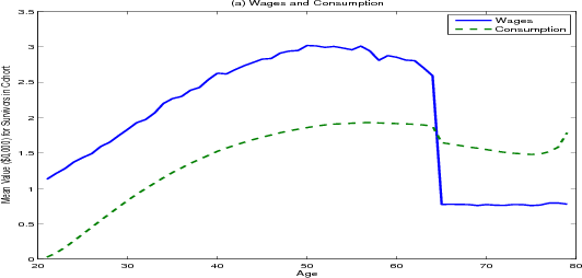
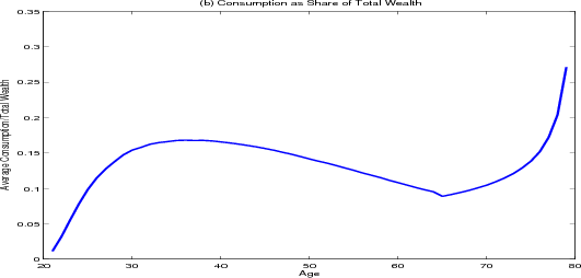
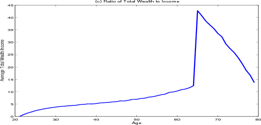
Income among surviving households drops sharply at retirement whereas the path of consumption over the life cycle is much smoother, (figure 4.1, panel A). Younger households who are aggressively saving for a down payment consume the smallest share of their wealth (panel B). Once households become homeowners, their consumption as a share of total wealth climbs, peaking near 16 percent around age 30. As households approach retirement, they start to accumulate more wealth, and consumption as a share of total wealth starts to fall, reaching a low of 9 percent at age 65 (panel C). In retirement, households draw down their savings, and consumption as a share of total wealth climbs again. At the outset of retirement the average household has roughly forty-five times its annual post-retirement income saved in both housing and financial wealth.
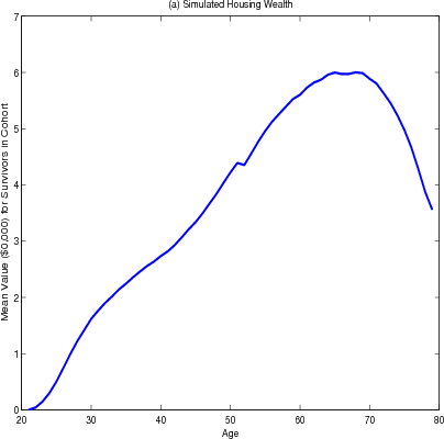
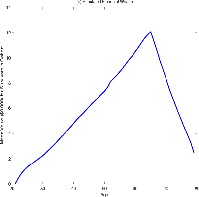
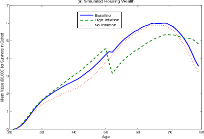
Housing wealth is hump-shaped, on average, over the life cycle of the household, reaching a peak at age 65 and declining after age 70 (figure 4.2 panel A). The brief plateau in the growth of housing wealth at age 50 is caused by many households either trading down to smaller homes or refinancing their existing mortgage to ensure that their nominal mortgage payments are fixed for the rest of their expected lives.1 Financial wealth over the life cycle is more sharply humped and peaks at age 65 (panel B).
Panel A reveals that households use accumulated home equity to finance their consumption of nondurables only late in retirement after their reserves of financial wealth have been largely depleted. These results are fairly consistent with some previous empirical work. Venti and Wise (2000) found that housing wealth was not in fact used to support non-housing consumption. They found that households resort to their home equity only when faced by a significant shock such as the death of a spouse or a serious illness. Similarly, Sheiner and Weil (1992) found that anticipation of illness or death significantly increases the probability that households will reduce their home equity. However, the present model does result in a more rapid decline late in life in housing wealth than previous empirical studies have shown. The model's omission and retiree labor supply might explain this failure. In particular households might view their home equity as an important source of savings to tap when faced with a serious health shock and be unwilling to extract that equity in the absence of such a shock. They could avoid consuming their housing wealth by continuing to work after retirement.
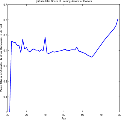
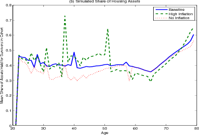
The simulated mean share of assets held in housing for surviving household heads between the ages of about 35 and 65 is consistently near 40 percent, (figure 4.2 panel C). The housing share is high among young households, who must invest a large portion of their savings in a down payment. As financial wealth grows faster than housing wealth, the housing share falls but somewhat climbs again. The jagged nature of the curve reflects a comparatively small number of simulations. The housing share climbs in retirement, as households draw down financial wealth before they extract home equity because of the transaction costs. This behavior can explain some of the "over investment" in housing seen in the empirical data, as reported by Flavin and Yamashita (2002). The implication is that some degree of over investment in housing can arise as a result of the mortgage contract rather than any suboptimal behavior by irrational consumers. Note, though, that the degree of over-investment implied by the model is below that seen in the data; Flavin and Yamashita find the mean share of total assets held in housing to be 67 percent.
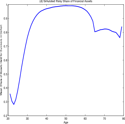
Regarding the allocation of financial assets over the life cycle, young households - who are focused on saving for a down payment or already have a large share of their wealth in housing - invest less in risky financial assets and more in the risk-free asset (figure 4.2 panel D). Older households also have their allocation weighted to less risky financial assets, but in their case because they have drawn down their financial wealth relative to their housing wealth. The share of the financial portfolio invested in risky assets peaks around age 50, just when households start to actively shift their total portfolio away from home equity.
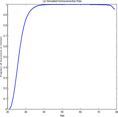
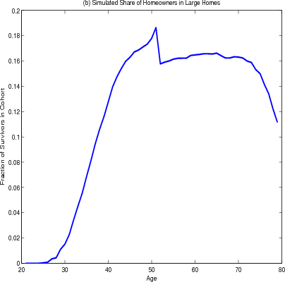
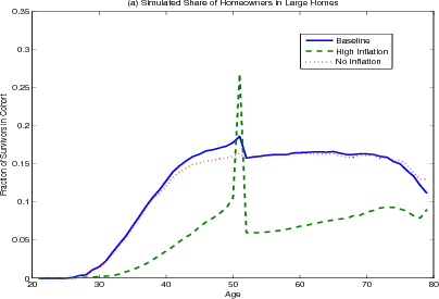
The model results also document other housing decisions over the life cycle. Homeownership increases rapidly for younger households and declines very slightly in retirement (figure 4.3 panel A). The share of homeowners living in larger homes has a similar contour with a considerable drop at age 50 (panel B), as households trade down in retirement to access housing wealth to finance consumption.
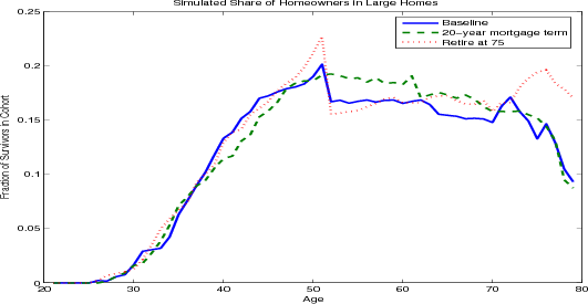
The sharpness of the decline at age 50 results largely from the combination of the thirty year term of the mortgage and the assumed maximum age of 80 and thus should not be taken too literally. In particular, at 50 years old, many households take advantage of the thirty year mortgage term to hold constant their nominal mortgage payments for the rest of their lives. These households will continue to receive a constant stream of utility from their home, the real value of the mortgage payments will fall because of inflation. In effect, in buying a home at age 50, households are purchasing an annuity from which the stream of real payments - the difference between the implicit rent and the real mortgage cost - will increase with time and be at its highest during retirement when income is at its lowest. This hypothesis is supported by results from simulations where the term of the mortgage is varied (figure 4.4). When the mortgage term is shortened to twenty years and the retirement age remains at 65, homeowners delay the shift to smaller homes to age 60. The results are not sensitive to the changing of the retirement age; in particular, when the retirement age is 75 and the mortgage term is thirty years, homeowners still shift to smaller homes at age 50. Thus proximity to retirement can be ruled out as a factor.
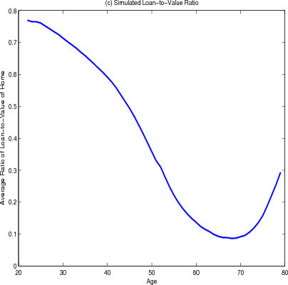
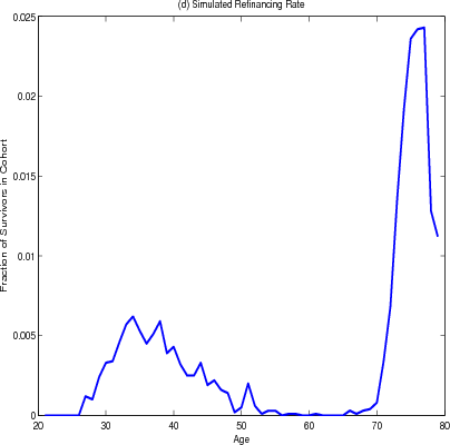
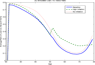
Panel C shows the path of the loan-to-value ration over the life-cycle. At the time they purchase their homes, households are required to have a loan-to-value ratio of 80 percent (panel C). They then pay down their mortgage through the regular amortization schedule and the average loan-to-value ratio falls. The average loan-to-value ratio seems to stabilize at 10% before climbing late in retirement in response to a surge in cash-out refinancing. This surge can be seen in Panel D. In addition, younger households and those that have just purchased their homes take advantage of refinancing to re-balance their portfolios and smooth their income.
5 The Effects of Inflation on Portfolio Allocation
This section shows how portfolio allocation across the life cycle changes with different levels of inflation. The model is re-solved for different levels and corresponding sets of simulations are generated. Setting the inflation parameter to a higher level simulates the effects of high inflation, and setting it to zero simulates the effect of mortgage contracts that are real rather than nominal. The levels of wealth accumulation, housing demand, refinancing activity, and portfolio allocation under each alternative assumption are then compared to the base case.
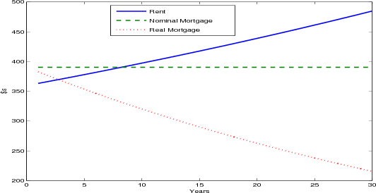
The presence of nominal mortgage contracts effectively shifts the real costs of home ownership forward over the term of the mortgage (figure 5.1). The fact that the real value of the mortgage payment declines over the life of the mortgage is, of course, factored into the original mortgage rate.
Figure 5.2 and 5.3 show how portfolio allocation and housing demand differ under different inflation rates. Under the zero-inflation scenario (the red-dotted lines) the transaction costs facing households in rebalancing their portfolios are significantly reduced. Households, especially younger households, hold less housing wealth. A common strategy in the presence of large transaction costs for durable goods is for a household to "over-buy," that is buy a larger house than they would otherwise, knowing that they would be unable to easily re-adjust their level of housing consumption later in the life-cycle when they might actually want a larger home. With zero inflation reducing the transaction costs, there is significantly less of this "over-buying." In addition, we do not observe the sudden shift towards smaller homes at age 50 seen in the base case, since the real value of the mortgage payment is no longer declining, and households gain less of a benefit of locking their mortgages prior to retirement.
The results from the high inflation scenario (the green lines) are a mirror image of those from the low inflation scenario. Now that the transaction costs associated with extracting home equity are higher, households rebalance their mortgage less frequently, resulting in an increase in housing wealth held by the young and very old and a decrease in housing wealth held by the middle-aged and early retirees.
The sudden shift towards smaller homes at age 50 is even more pronounced under the high inflation scenario, as the benefit of locking their mortgages prior to retirement is greater with higher inflation. Many households attempt to trade-up just prior at age 50, knowing that if they get several positive income shocks they would be able to afford the higher real mortgage payments, which would gradually decline over the life of the mortgage. When they do not receive positive income shocks, households in this model trade down because they fear they will not be able to make the mortgage payments once their income falls in retirement. During periods of high inflation, mortgage contracts with fixed nominal payments are especially attractive to households. During the prime of their earnings years (their 50s) the real mortgage payment is high. The real mortgage payment then falls rapidly during retirement, just when their income also falls. As discussed above, nominal mortgage payments allow older households to shift the expense of housing forward to earlier years to ensure their ability to consume housing later; the higher the rate of inflation, the greater the benefit to do so.
6 Conclusion
The model developed in this paper demonstrates the way in which perfectly anticipated inflation, even when reflected in the nominal interest rate on mortgages, can distort the household's portfolio allocation over the life cycle. A standard thirty-year fixed-rate nominal mortgage contract results in declining real mortgage payments. The longer a mortgage is held, the greater the difference between the household's mortgage payment and the payment for a mortgage refinanced in the current period. This widening gap discourages households from shifting assets from home equity to financial portfolios. When calibrated using commonly accepted parameters, the results can explain at least some of the "overinvestment in housing" documented in the earlier literature and also help explain why retired households hold such a significant portion of their wealth in housing.
Inflation distorts the household's portfolio allocation by introducing a hidden transaction cost through its effect on the real value of the fixed nominal mortgage payment. When inflation is high, the gap in the real value of a new mortgage and an existing mortgage is larger, and households rebalance their portfolio between home equity and financial assets less frequently. When inflation is low, household find extracting their home equity to be cheaper, and therefore more frequently rebalance their portfolio.
Appendix A - Detailed Partial Equilibrium Life Cycle Model
This appendix provides a detailed description of the partial equilibrium life-cycle model used in this paper. Aspects of the model that significantly differ from the basic model used in the literature are discussed in the main body of the paper.
The household's optimization problem is to maximize lifetime utility, defined as:
where
 represents the consumption of nondurables;
 represents the number of units of housing services consumed, given the housing tenure choice in period
  (note that while the number of units of housing services consumed varies with tenure choice, the utility gained from a unit of services does not vary);
 and
and  are the values of financial assets, home, and mortgage debt
left as bequests, respectively;
 represents the discount rate;
 is the survival probability;
 represents the measure of preference between a unit of housing and consumption;
 represents a measure of risk aversion; and
-
 and
and  represent parameters associated with the utility
of leaving bequests.
Households begin at age 20 as renters with no savings. Thus, they have no financial wealth and no housing wealth. In each period, a household receives a draw from an age-dependent income process. The model contains only transitory shocks. In retirement, pension income is set to 60 percent of the deterministic portion of income at age 65. Pension income is still subject to transitory shocks representing uncertainty regarding medical costs.
Households can store their wealth in two different classes of assets: financial and real. The household's financial assets are held in a portfolio of risk-free and risky assets. The household can costlessly rebalance its financial portfolio between risk-free and risky assets in every period.
Households with zero wealth face a binding liquidity constraint for financial assets in that they cannot borrow against their future income. The only way to effectively borrow against future income is through a mortgage for which the household meets the down payment and income requirements.
Households also cannot purchase leveraged portfolios, in which they borrow at the risk-free rate to invest more in risky assets. In addition to moving to one of the three types of housing, a rental unit (![]() ), a small house (
), a small house (![]() ), and a large house (
), and a large house (![]() ), the household
can also decide to stay in its current home,
), the household
can also decide to stay in its current home,
![]() . Households may add to their mortgage balance through cash-out refinancing.
. Households may add to their mortgage balance through cash-out refinancing.
The transition rule for the level of financial wealth is defined as:
where
 is the level of financial assets in period
  ;
; is a random variable that depends on the stochastic rate of return on risky assets (
 ) in period
  and the realizations of earnings (
 ) in period
  ;
; is the share invested in risky assets in time
  ;
; is the deterministic rate of return on risk-free assets;
-
 is the housing cost, that is the rent, or the mortgage plus maintenance and taxes, incurred in period
  for a household currently choosing tenure type
  with a mortgage
  years old;
 -
 is the mortgage interest paid;
 -
 is the net gain, that is, the proceed or cost from a housing transaction including the realized capital gain or loss from a sale and the down payment and
transaction costs from a new purchase, for a household choosing
  this period and
  next period;
 -
 is the net gain, that is, the value of home equity extracted after transaction costs, from cash-out refinancing; and
  is the tax rate on income and capital gains (note that both income and capital gains have the same tax rate and that taxes on capital gains are paid immediately).
Households receive their wages at the same time they realize the returns on their investment from the previous period. As a result, the state variable ![]() represents all available cash on
hand, consisting of previous financial wealth and current income. The income process is defined as a deterministic function of age plus a transitory shock:
represents all available cash on
hand, consisting of previous financial wealth and current income. The income process is defined as a deterministic function of age plus a transitory shock:
The real rate of return on risky assets is a random variable with the distribution
where
The value function of the household is the maximum utility, subject to the default constraints of the value functions for the households that choose next period's tenure type
![]() :
:
where
The value function conditional on next period's tenure choice ![]() is
is
such that equations (A-2) through (A-9) hold.
The code used to solve this problem was written in C. One solution of the problem initially took roughly two weeks on a dual processor Pentium Xeon 1.8GHz with 512K L2 cache and 1GB of RAM running Linux. In order to improve upon the run-time, the code was rewritten to take advantage of parallel processing, using the Message Passing Interface (MPI) standard. In this version of the code one processor is designated the master while a pool of other processors are designated slaves. As the model is solved recursively by year, the master distributes the current value function for all previous years to the slaves. Each slave then solves for the optimal value function for a subset of state spaces for the given year. The slaves then return the new value function values to the master. The master then combines the new values with the value function for the previous year, completing the recursion for one year. The problem was solved using 61 high-performance Digital Alpha 64-bit microprocessors running at 450MHz each on a scalable parallel Cray T3E at the Pittsburgh Supercomputing Center. One solution involved roughly 1.3 billion evaluations of the value function and took roughly eight and a half hours.
Appendix B - Baseline Model Parameter Values
The parameter values for the baseline model are chosen to be consistent with other models in the relevant literature. As was discussed in appendix A, the income process consists of a deterministic factor and a transitory factor. The income process is based on the results of regressions of Social Security earnings on age and age-squared. The dependent variable is the log of the wage income in constant 1990 dollars. The transitory factor of wage is reflected in the estimated standard error of the regression. The wage is converted from log to level terms in the model. At age 65 the level of the deterministic wage falls to a flat level equal to 60% of the last period's income before any transitory shocks, a condition representing a system of forced retirement and a defined benefit pension plan. The coefficients and standard deviation used in this version of the model are in Table B-1.
| Constant | 7.28626 | |
| Coefficient Age | 0.10278 | |
| Coefficient of Age |
-0.00098 | |
| Std. Dev. | 0.80778 | |
| R |
15.5% | |
| Probability of Unemployment | 1% |
The market price of a housing unit is the result of setting the deterministic home price at age 60 with the National Association of Realtors' 1990 median home price. It is assumed that a median home consists of 10 housing units. The home prices are converted to constant 1990 dollars and the deterministic home price series are calculated using the historical average return. The average and standard deviation of the return on housing are at taken from Li and Yao (2004) and are consistent with Campbell and Cocco (2003). The mortgage interest rate used is the average rate on loans with 80 percent loan-to-value ratios as reported by Freddie Mac from 1969 to 2001, adjusting for the inflation rate. The percent required for the down payment represents the minimum needed to avoid paying mortgage insurance. The transaction, maintenance, and moving costs are based on survey data provided by the National Association of Realtors. The values chosen for the current version of the model are in Table B-2. The risk and return on risky assets follows Yao and Zhang (2004).
| Parameter Name and Definition | Symbol | Value |
|---|---|---|
| Real risk free rate of return | r | 2% |
| Price of 1 housing unit, at age 60 | 1.003 | |
| Size of small homes | 8 | |
| Size of large homes | 12 | |
| Mean of real return on housing | 1% | |
| Standard deviation of housing return | 11.5% | |
| Mean of real return on risky asset | 6% | |
| Standard deviation of risky asset return | 15.7% | |
| Probability of 100% loss on risky asset | 1% | |
| Mortgage interest rate | 5% | |
| Percent required as down payment | 20% | |
| Percent of home price lost to transaction costs | 10% | |
| Maintenance costs | 0.7% | |
| Moving costs | 0.3 | |
| Tax Rate | 30% | |
| Refinancing Costs | 3% | |
| Inflation | 2% |
The values for the preference parameters shown in Table B-3 below were chosen to replicate certain stylized facts about the role of owner-occupied housing in portfolios, specifically the large share of total wealth held in home equity. An ![]() value of 2 represents a relatively low, but realistic, level of risk aversion. An
value of 2 represents a relatively low, but realistic, level of risk aversion. An ![]() value of 0.96
is a commonly used discount rate. The
value of 0.96
is a commonly used discount rate. The ![]() value of 0.2 reflects the share of total household expenditures allocated to housing expenditures in the 2001 Consumer Expenditure Survey from the
U.S. Department of Labor. The discount rate for bequests are 0.8 for
value of 0.2 reflects the share of total household expenditures allocated to housing expenditures in the 2001 Consumer Expenditure Survey from the
U.S. Department of Labor. The discount rate for bequests are 0.8 for ![]() , 0.8 for
, 0.8 for ![]() , and 0.8 for
, and 0.8 for ![]() . They are chosen to imply that households would rather consume one additional dollar than leave an additional dollar as a bequest and that
households place a premium on leaving their homes as bequests relative to other assets.
. They are chosen to imply that households would rather consume one additional dollar than leave an additional dollar as a bequest and that
households place a premium on leaving their homes as bequests relative to other assets.


