Inflation Persistence, Backward-Looking Firms, and Monetary Policy in an Input-Output Economy*
Keywords: Inflation persistence, intermediate goods, monetary policy
Abstract:
This paper studies the implications of inflation persistence (generated by backward-looking price setters) for monetary policy in a New Keynesian "input-output" model--a model with sticky prices in both intermediate and final goods sectors. Optimal policy under commitment depends on the degree of inflation persistence in both sectors. Under discretion, speed-limit targeting--targeting the change in the output gap--outperforms price-level and inflation targeting in the presence of inflation persistence. If inflation persistence is low in the intermediate goods sector, price-level targeting outperforms inflation targeting despite high inflation persistence in the final goods sector.
JEL codes: E50, E52, E58
1 Introduction
How should monetary policy be conducted in a New Keynesian model in which prices are sticky at multiple stages of production? Huang and Liu (2005) and Strum (2009) examine this question using a forward-looking New Keynesian "input-output" model--a model that has sticky prices in both the intermediate and final goods sectors. They find that a central bank paying attention to price movements in both the final and intermediate goods sectors can more ably minimize household utility losses than if it considers only one sector. Furthermore, Strum (2009) finds that if the central bank acts under discretion, it performs better if it targets price levels rather than inflation rates.
One feature of the standard forward-looking New Keynesian framework is that it generates Phillips curves that do not relate current inflation to lagged inflation. Yet studies such as Fuhrer (1997), Rudebusch (2002), and Roberts (2005) find an important empirical role for lagged inflation in the Phillips curve. Besides affecting the specification of the Phillips curve, inflation persistence can affect the evaluation of monetary policy in New Keynesian models. For example, when examining discretionary monetary policy regimes in one-sector New Keynesian models, Walsh (2003) and Nessén and Vestin (2005) show that the type of regime that performs best depends on the degree of inflation persistence in the Phillips curve.
These findings suggest the question: How is monetary policy design in a New Keynesian input-output model affected by inflation persistence? To answer this question, the standard model must be extended so that the Phillips curve exhibits inflation persistence. As recent scholarship has found, inflation persistence can arise in New Keynesian models in a number of different ways.1 This paper builds inflation persistence into the input-output model developed by Huang and Liu (2005) and extended in Strum (2009) by following the approach pioneered in Galí and Gertler (1999), Amato and Laubach (2003), and Steinsson (2003): When resetting prices, some firms are modeled as employing a simple rule of thumb that uses information about past states of the world to set new prices. These firms may behave this way if, from time to time, they find it too costly to gather new information and calculate the optimal forward-looking price. Firms using this rule of thumb generate inflation persistence in the sectoral Phillips curves. Furthermore, compared to models with sticky prices in one sector, this model can yield different degrees of inflation persistence in different sectors.
This paper examines four questions about monetary policy in New Keynesian models: How does inflation persistence at multiple stages of production affect the conduct of optimal policy under commitment? How does inflation persistence at multiple stages of production affect the type of loss function that should be assigned to a central bank acting under discretion? How well do different regimes perform when policies are set using incorrect assumptions about inflation persistence or the sources of shocks? How well do policies derived from one-sector models perform when implemented in an input-output model?
I find that the timing and magnitude of the central bank's responses to shocks when implementing optimal monetary policy under commitment are affected not only by the presence of inflation persistence, but also by the relative degrees of sectoral inflation persistence. On the other hand, the nature of the central bank's responses--whether expansionary or contractionary--is not affected by the degrees of inflation persistence.
When studying monetary policy under discretion, I find that inflation persistence affects the type of loss function that best minimizes household losses. As in Strum (2009), price-level targeting performs best in a forward-looking model. However, when inflation persistence is introduced, speed-limit targeting (a regime targeting the change in the output gap) performs best. Price-level targeting outperforms inflation targeting unless inflation persistence is high in both sectors.
When a regime is chosen and the loss function is crafted, the government may make an incorrect assessment of inflation persistence in the two sectors, the sources of shocks, or the need to use the input-output model. I find that, given the degrees of inflation persistence in the two sectors, the type of regime that performs best is not affected by the government's assumptions regarding inflation persistence or the sources of shocks (when crafting the loss function). However, the type of regime that performs best is affected by the incorrect use of a one-sector model.
The remainder of the paper is organized as follows: Section 2 sets up the model and presents the linearized version used for later analysis. Section 3 discusses the calibration. Section 4 examines the qualitative characteristics of optimal policy under commitment for different degrees of inflation persistence in the two sectors. Section 5 compares the performances of simple loss functions under the more realistic case of discretionary optimization. Section 6 examines some robustness properties of the discretionary regimes. Section 7 concludes.
2 Model of an Input-Output Economy
Huang and Liu (2005) develop a New Keynesian model with a vertical production chain consisting of two sectors. Firms in the first sector produce final (nondurable) goods using intermediate goods and labor. Final goods are consumed by households. In the second sector, intermediate (nondurable) goods are produced using only labor. Intermediate goods are used only by final goods firms in production. Each firm in each sector produces a unique differentiated good and engages in monopolistic competition within its sector. Prices in both sectors are sticky, and firms adjust their prices in a staggered manner in the spirit of Calvo (1983). There is one competitive market for homogenous labor that can be used by all firms. All firms are price takers in their input markets.
Strum (2009) extends the model by introducing cost-push shocks and characterizing monetary policy as the minimization of an assigned loss function. This paper extends the model in Strum (2009) by assuming that in each sector and in each period, a fraction of firms find that solving for the optimal forward-looking price is too costly. Following Galí and Gertler (1999), Amato and Laubach (2003), and Steinsson (2003), I assume that backward-looking firms in each sector employ a rule of thumb that uses past information to set a new price. This section presents the basic elements of the model and its linearized version used for subsequent analysis.2
2.1 Households
The economy is populated by a large number of identical, infinitely lived households. Households derive utility from consumption and leisure. Given a fixed amount of time that households divide fully between leisure and labor each period, the household utility function can be written in terms of labor instead of leisure. Accordingly, households maximize expected lifetime utility, given by
![\displaystyle E_{0}\left\{ \sum_{t=0}^{\infty}\beta^{t}\left[ u\left( C_{t}\right) -v\left( N_{t}\right) \right] \right\} ,](img1.gif) |
(1) |
where
The period utility function for consumption is
![]() . The consumption good,
. The consumption good, ![]() , is a
composite of a continuum of differentiated final goods in the spirit of Dixit and Stiglitz (1977), given by
, is a
composite of a continuum of differentiated final goods in the spirit of Dixit and Stiglitz (1977), given by
![\displaystyle C_{t}\equiv\left[ \int_{0}^{1}y_{ft}\left( i\right) ^{\left( \theta _{ft}-1\right) /\theta_{ft}}\,di\right] ^{\theta_{ft}/\left( \theta _{ft}-1\right) }](img7.gif) , , |
(2) |
where
Households have equal ownership in all firms and divide all profits equally among themselves. Labor is homogeneous and supplied equally by households to all firms through one market with one wage rate, which households take as given. I assume complete financial markets. Finally, I assume standard budget-set and transversality conditions hold.
2.2 Final Goods
Each final goods firm ![]() has access to a constant returns to scale (CRS) Cobb-Douglas production function
has access to a constant returns to scale (CRS) Cobb-Douglas production function
| (3) |
where
![\displaystyle Y_{mt}\left( i\right) \equiv\left[ \int_{0}^{1}y_{mt}\left( i,j\right) ^{\left( \theta_{mt}-1\right) /\theta_{mt}}\,dj\right] ^{\theta _{mt}/\left( \theta_{mt}-1\right) }](img18.gif) , , |
(4) |
where
Each firm minimizes costs to meet the demand for its good given its stated price. Final goods firms adjust their prices with probability
![]() each period, where
each period, where
![]() . A random fraction
. A random fraction
![]() of firms resetting prices find it worthwhile to determine the price that maximizes discounted expected profits over the time the price is expected to persist, where
of firms resetting prices find it worthwhile to determine the price that maximizes discounted expected profits over the time the price is expected to persist, where
![]() . This maximization problem is given by
. This maximization problem is given by
where
The remaining fraction ![]() of firms setting a new price use a rule of thumb to determine a new backward-looking price,
of firms setting a new price use a rule of thumb to determine a new backward-looking price,
![]() , instead of solving an explicit optimization problem. Steinsson (2003) suggests a generalization of the Galí and Gertler (1999) approach by allowing firms to also react to
an indicator of the previous period's output gap. Generalizing the rule of thumb in Steinsson (2003), I assume that the backward-looking firms set prices according to
, instead of solving an explicit optimization problem. Steinsson (2003) suggests a generalization of the Galí and Gertler (1999) approach by allowing firms to also react to
an indicator of the previous period's output gap. Generalizing the rule of thumb in Steinsson (2003), I assume that the backward-looking firms set prices according to
where
Galí and Gertler (1999) formulate a rule similar to the one above, except they effectively set
where
The aggregate price level can be written as
2.3 Intermediate Goods
Each intermediate goods firm ![]() has access to a CRS production function given by
has access to a CRS production function given by
| (10) |
where
2.4 Government
The government serves two purposes in this model. First, it assigns a loss function to an independent central bank. The central bank acts to minimize its assigned loss function. I assume that the central bank can react to and affect state variables in the current period. Second, the government collects lump-sum taxes from households to provide subsidies to firms so that the steady-state equilibrium is not distorted from inefficiencies arising from monopolistic competition. Finally, I ignore the possible interactions between monetary and fiscal policy that would be present in a richer model.
2.5 Linearized Model
I log-linearize the model using log-deviations from a hypothetical non-distorted efficient equilibrium (the equilibrium that would obtain if prices were flexible and there were no shocks to the elasticities of substitution).4 The natural rate of interest is the real interest rate that would obtain in the efficient equilibrium. I list the key variables and symbols from the model in Table 1.
The household intertemporal consumption equation is obtained from the household's first-order conditions. Its log-linearized version is given by
I interpret
The log-linearized pricing equations for backward-looking firms can be combined with the log-linearized first-order equations for forward-looking firms to obtain Phillips curves for each sector, namely,
| (12) | ||
| (13) | ||
where, for
![\displaystyle =\frac{\left( 1-\alpha_{k}\right) \left[ \left( 1-\alpha_{k}\beta\right) \left( 1-\iota_{k}\right) -\alpha_{k}\beta \iota_{k}\delta_{k}\right] }{\iota_{k}\left( 1-\alpha_{k}+\alpha_{k} \beta\right) +\alpha_{k}},](img101.gif) |
||
 |
||
![\displaystyle =\frac{\left( 1-\alpha_{k}\beta\right) \left( 1-\iota_{k}\right) \left( 1-\alpha_{k}\right) }{\left( 1-\bar{\theta}_{k}\right) \left[ \iota_{k}\left( 1-\alpha_{k}+\alpha_{k}\beta\right) +\alpha_{k}\right] }\hat{\theta}_{kt}](img105.gif) . . |
As noted in Section 2, though
The sectoral Phillips curves reveal how the percentage of backward-looking firms affects the sectoral Phillips curves. An increase the percentage of backward-looking firms increases the weight of lagged inflation relative to the forward-looking component (
![]() is decreasing and
is decreasing and
![]() is increasing in
is increasing in ![]() ). The coefficient of the sectoral Phillips
curves with respect to the sector's current real marginal cost gap (and, therefore, the output gap) decreases as the percentage of backward-looking firms increases (
). The coefficient of the sectoral Phillips
curves with respect to the sector's current real marginal cost gap (and, therefore, the output gap) decreases as the percentage of backward-looking firms increases (
![]() is decreasing in
is decreasing in ![]() ).5 On the other hand, the coefficient of the sectoral Phillips curves with respect to the sector's lagged real marginal cost gap increases as the percentage of backward-looking firms increases (
).5 On the other hand, the coefficient of the sectoral Phillips curves with respect to the sector's lagged real marginal cost gap increases as the percentage of backward-looking firms increases (
![]() is increasing in
is increasing in ![]() ).
).
The weight on intermediate goods in the production function of final goods, represented by ![]() , affects the coefficients of the current and lagged output gaps in the final goods
Phillips curve, given by
, affects the coefficients of the current and lagged output gaps in the final goods
Phillips curve, given by
![]() and
and
![]() , respectively. As in the forward-looking model in Strum (2009), higher values of
, respectively. As in the forward-looking model in Strum (2009), higher values of ![]() correspond to lower values of the coefficient of the current output gap in the final goods Phillips curve. Moreover, higher values of
correspond to lower values of the coefficient of the current output gap in the final goods Phillips curve. Moreover, higher values of ![]() also correspond to lower values of the coefficient of the lagged output gap in the final goods Phillips curve.6
also correspond to lower values of the coefficient of the lagged output gap in the final goods Phillips curve.6
In standard hybrid New Keynesian Phillips curves, the cost-push shocks are represented by terms like ![]() . In this model, the term
. In this model, the term ![]() arises from
arises from
![]() , variations in the elasticities of substitution of differentiated goods. The magnitude of a one-standard-deviation shock to
, variations in the elasticities of substitution of differentiated goods. The magnitude of a one-standard-deviation shock to
![]() does not depend on the percentage of backward-looking firms. However, as the expression for
does not depend on the percentage of backward-looking firms. However, as the expression for ![]() shows, the effects of fluctuations in the elasticities of substitution are attenuated by higher percentages of backward-looking firms. For the state-space representation of the model, I rewrite this term as
shows, the effects of fluctuations in the elasticities of substitution are attenuated by higher percentages of backward-looking firms. For the state-space representation of the model, I rewrite this term as
| (14) |
where
As noted in Table 1, the "relative price" refers to the ratio of the price index for intermediate goods to the price index for final goods. The relative price gap evolves, by definition, according to
| (15) |
I assume that the technology factors are stationary--that is,
| (16) |
where, for sector
In this model, the nominal interest rate does not appear in the objective function of the central bank and is not a constraint in the central bank's maximization problem. Therefore, I simplify the setup by treating
![]() as the instrument of the central bank. Once the model is solved, I use (11) to determine the interest rates that are consistent with the desired equilibrium.
I compute price levels using the identity
as the instrument of the central bank. Once the model is solved, I use (11) to determine the interest rates that are consistent with the desired equilibrium.
I compute price levels using the identity
![]() for
for
![]() , where
, where ![]() can be interpreted as the log-deviation in
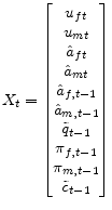
the price level from its initial value. I represent the structural equations of the economy as
can be interpreted as the log-deviation in
the price level from its initial value. I represent the structural equations of the economy as
where
 ,
,  ,
,  .
.2.6 Household Loss Function
The second-order Taylor approximation to the household's utility function is given by
 E E t.i.p. t.i.p. |
(18) |
where
| (19) | ||
with coefficients
 |
||
 |
||
 |
||
 |
||
 |
||
 |
||
 |
||
 ,
, |
where
The period loss function is a natural extension of period loss functions in other models. Under the assumption of one sector with sticky prices, the first line of the period loss function is obtained. The assumption that both intermediate and final goods sectors have sticky prices adds the
second line. The third line is obtained if backward-looking price setters are included and
![]() (the formulation in Galí and Gertler, 1999). The last two lines of the loss function arise if backward-looking firms react to past marginal cost gaps in their rule of
thumb.
(the formulation in Galí and Gertler, 1999). The last two lines of the loss function arise if backward-looking firms react to past marginal cost gaps in their rule of
thumb.
Inflation in each sector corresponds to lower household utility since the interaction of sticky prices and inflation produces a set of suboptimal relative prices of differentiated goods, which then leads to inefficient mixes of goods in each sector. In the loss function, the real marginal cost gap in the intermediate goods sector is connected to the relative price's role in the allocation of resources across sectors. Finally, as is standard in other models, deviations of consumption (final output) from the efficient level correspond to higher utility losses.
In order to understand the connection between the household loss function and the proportion of backward-looking price setters, I present the loss function weights for a number of combinations of forward-looking and backward-looking price setters in Table 2. The calibration of the model
determining these weights is explained in Section 3. The main effect of backward-looking price setters is a dramatic increase in the importance of smoothing the change of inflation, represented by ![]() and
and ![]()
|
3 Calibration of the Model
This section discusses the calibration used for the benchmark model. The assumption that
![]() implies that
implies that ![]() . I set the
subjective time discount factor to
. I set the
subjective time discount factor to
![]() , implying that the annual real interest rate in the steady state is about 4 percent, given that I interpret a time period as a quarter. The steady-state values of the
elasticities of substitution for the differentiated goods,
, implying that the annual real interest rate in the steady state is about 4 percent, given that I interpret a time period as a quarter. The steady-state values of the
elasticities of substitution for the differentiated goods,
![]() and
and
![]() , are set to 10, which implies a steady-state markup of about 11 percent. Consistent with earlier empirical work (e.g., Carlton, 1986; and Blinder et al., 1998) and following
Huang and Liu (2005) and Strum (2009), I set the average price contract equal to one year, which means setting
, are set to 10, which implies a steady-state markup of about 11 percent. Consistent with earlier empirical work (e.g., Carlton, 1986; and Blinder et al., 1998) and following
Huang and Liu (2005) and Strum (2009), I set the average price contract equal to one year, which means setting
![]() . I also follow Huang and Liu (2005) and Strum (2009) in setting
. I also follow Huang and Liu (2005) and Strum (2009) in setting
![]() .
.
Technology shocks are typically represented as small but persistent (see, for example, Cooley and Prescott, 1995, and Gomme and Rupert, 2007). I set the AR(1) coefficients for process governing the evolution of the technology factors to
![]() . I set the standard deviation of the innovations to the technology factor process in each sector,
. I set the standard deviation of the innovations to the technology factor process in each sector,
![]() , to 0.02.
, to 0.02.
As noted earlier, I assume that the cost-push shocks are white noise processes that do not depend on ![]() . I set
. I set
![]() so that the standard deviation of
so that the standard deviation of ![]() is
is ![]() in the purely forward-looking case. I chose this value so that a negative two-standard-deviation shock does not cause the central bank to hit the zero bound on the nominal interest rate when
implementing optimal policy with commitment.9 When
in the purely forward-looking case. I chose this value so that a negative two-standard-deviation shock does not cause the central bank to hit the zero bound on the nominal interest rate when
implementing optimal policy with commitment.9 When
![]() , I use the expressions for
, I use the expressions for ![]() derived earlier to adjust
derived earlier to adjust
![]() .
.
As I am not aware of any models with estimates of
![]() , I set these values so that the coefficient on lagged marginal cost in the backward-looking rule of thumb equals that of the coefficient on current marginal cost in the Phillips
curves in which there are no backward-looking price setters (similar to the approach in Steinsson, 2003). This leads me to set
, I set these values so that the coefficient on lagged marginal cost in the backward-looking rule of thumb equals that of the coefficient on current marginal cost in the Phillips
curves in which there are no backward-looking price setters (similar to the approach in Steinsson, 2003). This leads me to set
![]() .
.
A number of authors have fit empirical estimates to hybrid Phillips curves. Fuhrer (1997) finds that setting more relative weight on lagged inflation does better, whereas Galí and Gertler (1999) find that more weight should be put on the forward-looking term. I take a middle-of-the-road
approach and set
![]() , implying
, implying
![]() and
and
![]() in (12), which is in line with the estimates in Roberts (2005). Since Clark (1999) finds that the prices of goods at earlier stages of processing are
more responsive to monetary policy shocks, I assume that the intermediate goods sector does not have greater persistence than the final goods sector. Consequently, I set
in (12), which is in line with the estimates in Roberts (2005). Since Clark (1999) finds that the prices of goods at earlier stages of processing are
more responsive to monetary policy shocks, I assume that the intermediate goods sector does not have greater persistence than the final goods sector. Consequently, I set ![]() equal to or
less than
equal to or
less than ![]() , with three possible values for
, with three possible values for ![]() :
: ![]() and 0.7.
and 0.7.
4 Optimal Policy with Commitment
In this section, I assume that the central bank is assigned the household loss function. Furthermore, I assume that the central bank can credibly commit to state-contingent future actions. The intertemporal loss function of the central bank is given by
E . . |
(20) |
Without loss of generality, I have multiplied the household loss function by
| (21) |
where
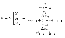 .
. |
(22) |
The matrices

|
(23) | |
 , , |
where
 and
and The results in Section 2 show that inflation persistence affects the model in three ways that matter for policymakers: First, higher inflation persistence in a particular sector causes the household utility function to put more weight on smoothing inflation in that sector. Second, for the calibrations considered in this paper, a higher degree of sectoral inflation persistence leads to a flatter sectoral Phillips curve with respect to the output gap.12 Third, higher sectoral inflation persistence means that policymakers must work against a greater degree of momentum when attempting to affect sectoral inflation.
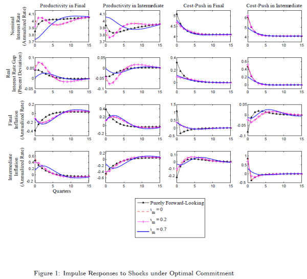
How do these additional complications arising from inflation persistence affect optimal policy under commitment? Figure 1 presents the optimal commitment responses to positive shocks under different combinations of sectoral inflation persistence. The standard forward-looking case is obtained by
setting
![]() . Two cases of high final goods inflation persistence and low intermediate goods inflation persistence are obtained by setting
. Two cases of high final goods inflation persistence and low intermediate goods inflation persistence are obtained by setting
![]() and
and
![]() or 0.2. Finally, high inflation persistence in both sectors is
obtained by setting
or 0.2. Finally, high inflation persistence in both sectors is
obtained by setting
![]() .
.
The first and second columns of Figure 1 show the central bank's responses to positive one-standard-deviation productivity shocks. The top row shows the (annualized) values of the nominal interest rate that are consistent with the central bank's policy. However, the real interest rate gap, shown in the second row, indicates the nature of monetary policy (whether policy is expansionary or contractionary).
Initially, a positive productivity shock in the final goods sector induces the central bank to enact contractionary policy (a positive real interest rate gap), whereas the central bank pursues expansionary policy (a negative real interest rate gap) in response to a positive productivity shock in the intermediate goods sector. The nature of the central bank's response does not depend on the degrees of inflation persistence in the two sectors.
However, the timing and magnitude of the central bank's responses to productivity shocks depend on the degrees of inflation persistence in the two sectors. When inflation persistence is high in the final goods sector but low in the intermediate goods sectors, the central bank delays its maximal response and increases the magnitude of its maximal response. When inflation persistence is high in both sectors, the central bank also delays its maximal response relative to the forward-looking case; however, unlike the case of unequal inflation persistence, the maximal response is of lesser magnitude than in the forward-looking case. Finally, the bottom two rows show that when a sector is populated by a large number of backward-looking price setters, inflation (or deflation) in that sector has a delayed and muted maximal response to a productivity shock in either sector.
The third and fourth columns of Figure 1 show the dynamics following positive one-standard-deviation cost-push shocks. The simulations show that, unlike the case with productivity shocks, the central bank engages in contractionary policy when responding to positive cost-push shocks in either sector. On the other hand, just as is the case with productivity shocks, the nature of the response does not depend on the degrees of inflation persistence in the two sectors.
The timing of the central bank's maximal response to a cost-push shock does not depend on the degrees of inflation persistence in the two sectors; however, the magnitude does. The maximal response comes in the initial period whether or not inflation is persistent. The magnitude of the central bank's response to a cost-push shock is strongly affected by the attenuation of the effect of cost-push shocks on sectoral inflation that occurs as the percentage of backward-looking firms in a sector increases. Accordingly, the magnitude of the central bank's maximal response to a cost-push shock decreases noticeably relative to the forward-looking case if inflation persistence is high in the sector hit by the shock. Finally, as the bottom two rows show, when a sector is characterized by high inflation persistence, the magnitude of the initial jump in inflation (or deflation) in that sector following a cost-push shock in either sector is lower than in the forward-looking case.
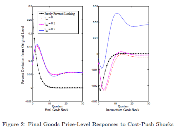
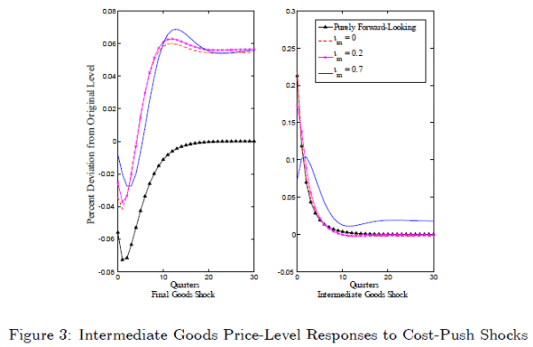
Figures 2 and 3 show that the behavior of the price levels of final and intermediate goods following positive one-standard-deviation cost-push shocks depends on the percentage of backward-looking price setters in the sector hit by the shock. So, for example, the response of the price level of final goods to a cost-push shock in the intermediate goods sector depends critically on the number of backward-looking firms in the intermediate goods sector. Consistent with Steinsson (2003), the price levels of both sectors do not return to their pre-shock levels if there are backward-looking price setters. However, if the intermediate goods sector has few backward-looking price setters, the price levels of both sectors converge to levels very close to their pre-shock values following a cost-push shock in the intermediate goods sector. Furthermore, even when inflation persistence is high in the intermediate goods sector, the magnitudes of the permanent effect of an intermediate goods cost-push shock on price levels in both sectors are lower than if the shock occurred in the final goods sector (when persistence is high in the final goods sector). Given that previous studies have found that price-level targeting under discretion works well in the forward-looking case, Figures 2 and 3 suggest that price-level targeting may perform well in an input-output model with inflation persistence, especially if the intermediate goods sector has fewer backward-looking firms, is more likely to experience cost-push shocks than the final goods sector, or has both of these characteristics.
5 Discretionary Policy Regimes
Although an analysis of the optimal commitment policy is useful for understanding the characteristics of desirable policy, Clarida, Galí, and Gertler (1999) point out that central banks do not make binding commitments. Furthermore, simple loss functions are easier for the public to understand and monitor, facilitating transparency and communication. Accordingly, I examine household utility losses that arise under alternative simple loss functions assigned to central banks acting under discretion. I consider the same combinations of inflation persistence as in the previous section and examine three classes of loss functions: inflation targeting (IT), price-level targeting (PT), and speed-limit targeting (SL). I also report household losses under the optimal commitment policy (COM).
Under inflation targeting, the central bank acts to keep inflation and other variables (such as the output gap) close to a set of target values.13 Price-level targeting differs from inflation targeting in that the central bank reacts to deviations of the price level from a target value. Speed-limit targeting stabilizes fluctuations in the change in the output gap in addition to other target variables. In a forward-looking model, Strum (2009) finds that targeting inflation or price levels in both sectors dominates single-sector targeting regimes; therefore, I consider only regimes that target inflation or price levels in both sectors.
I represent these regimes by loss functions given by
The government sets the weights
One disadvantage of the backward-looking rule is that optimizing agents might not use the same backward-looking rule in different regimes. Nevertheless, two factors suggest that the approach in this paper is useful. First, although different regimes lead to different short-run dynamics of inflation, all of the regimes are consistent with the same steady-state inflation rate of zero. Second, firms do not adopt the rule to optimize or as a long-term rule, but rather at random times when information costs are high. Therefore, the backward-looking rule can be seen as a simple rule employed by firms when they occasionally find the costs of information gathering and processing prohibitively expensive.
The central bank's problem can be put in a standard linear-quadratic setup.15 I calculate and report the expected household losses under each loss function as
![\displaystyle \bar{C}=100\frac{\text{E}\left[ \mathcal{L} ^{regime}\right] }{u_{C}\left( \bar{C}\right) \bar{C}}\text{,}](img252.gif)
Table 3 reports the coefficients and expected household losses for each regime according to the percentages of backward-looking firms (and, hence, degrees of inflation persistence) in the two sectors.17 Two observations jump out immediately. First, the absolute levels of losses are highest in the fully forward-looking model and lowest in the model with high persistence in both sectors. When the percentage of backward-looking price setters is high, the attenuation of the effects of cost-push shocks in the sectoral Phillips becomes important. Second, even though there is always a clear ranking of regime performance, the difference between the best and worst regimes decreases as inflation persistence increases.
|
|
The qualitative results are summarized in Table 4. Consistent with Strum (2009), price-level targeting produces the lowest household losses in the purely forward-looking model. When inflation persistence is high in the final goods sector but low in the intermediate goods sector, speed-limit targeting performs best. At the same time, price-level targeting outperforms inflation targeting. When inflation persistence is high in both sectors, speed-limit targeting performs best. However, in this instance, inflation targeting performs better than price-level targeting (and only slightly worse than speed-limit targeting). These results are broadly consistent with Walsh (2003), who finds that speed-limit targeting outperforms price-level targeting once moderate levels of inflation persistence are reached, and that inflation targeting performs well when inflation persistence is high. However, these results show that the degrees of inflation persistence in both intermediate and final goods sectors can be important when ranking regime performance.
|
6 Robustness of Discretionary Regimes
In the previous section, the government crafted loss functions based on an accurate assessment of inflation persistence, the sources of shocks to the economy, and the model of the economy to be used. However, monetary policy may not be practiced in such favorable conditions. In this section, I examine how discretionary regimes perform when the central bank minimizes loss functions that were crafted based on assumptions that may not be true.
6.1 The Degrees of Inflation Persistence
I begin by examining how policies crafted under incorrect assumptions about inflation persistence perform. Specifically, I follow a two-step process: First, I assume that the government chooses loss function coefficients based on assumptions regarding inflation persistence in each sector that
may not be accurate. Second, I determine the household losses that occur when the central bank implements these policies in the true economy. Table 5 reports the results from this exercise. For example, in the block of columns under "![]() ," the table shows the household losses for policies crafted under four assumed combinations of degrees of inflation persistence, and implemented in a forward-looking world.
," the table shows the household losses for policies crafted under four assumed combinations of degrees of inflation persistence, and implemented in a forward-looking world.
Price-level targeting performs best in the forward-looking world in three of the four scenarios. When inflation is persistent in the final goods sector but forward-looking in the intermediate goods sector, price-level targeting performs best in two of the four scenarios, while speed-limit targeting performs best in the other two scenarios. When inflation persistence is high in the final goods sector and either low (but positive) or high in the intermediate goods sector, speed-limit targeting performs best. Although inflation targeting never performs best, it outperforms price-level targeting in three of the four scenarios when inflation persistence is high in both sectors. Finally, as the true levels of inflation persistence rise, the losses from making the wrong assumptions about the degrees of inflation persistence decrease.
|
|
6.2 The Sources of Shocks
Next, I examine regime performance when the loss function is based on the assumption that shocks hit either only the final goods sector or only the intermediate goods sector, when, in fact, shocks hit both sectors. I assume that the government correctly perceives the degrees of inflation
persistence in both sectors when it sets the loss functions. I follow a two-step process similar to the one above: I calibrate loss function coefficients that are optimal under the assumption that shocks hit only one of the sectors, then I run the implied policies in economies that are subject to
shocks in both sectors. Table 6 reports the results for the four possible combinations of inflation persistence. The columns labeled "F" show the results when the central bank is assigned a loss function based on the assumption that shocks arise only in the final goods
sector. The columns labeled "M" show the results when the loss function is based on the assumption of shocks coming only from the intermediate goods sector. For example, in the two-column block under "![]() ," the column labeled "F" shows the household losses under regimes based on the assumption that shocks hit only the final goods sector, when, in fact, shocks hit both sectors.
," the column labeled "F" shows the household losses under regimes based on the assumption that shocks hit only the final goods sector, when, in fact, shocks hit both sectors.
If the government crafts the loss function based on the incorrect assumption that shocks hit only one sector, better results are usually obtained if the government assumes that shocks hit the intermediate goods sector. Regardless of which sector is assumed to be hit by shocks, price-level targeting performs best in the forward-looking case. When inflation persistence is high in the final goods sector and either low or high in the intermediate goods sector, speed-limit targeting performs best. Although inflation targeting ranks last both when the economy is fully forward-looking and when inflation persistence is high in the final goods sector but low in the intermediate goods sector, it outperforms price-level targeting when inflation persistence is high in both sectors.
|
6.3 Assumption of a One-sector Model
Finally, suppose that the central bank is assigned a loss function based on a standard one-sector model in which inflation is assumed to be final goods inflation. I consider two alternatives: a loss function based on a forward-looking one-sector model and a loss function based on a one-sector
model with many backward-looking price setters. Table 7 reports the household losses when these policies are implemented in the four input-output economies examined in earlier sections. For example, in the two-column block under "![]() ," the column labeled "0" shows the household losses under regimes based on the assumption of a one-sector model with no inflation persistence, when the true economy has an input-output
structure with high inflation persistence in the final goods sector and no inflation persistence in the intermediate goods sector.
," the column labeled "0" shows the household losses under regimes based on the assumption of a one-sector model with no inflation persistence, when the true economy has an input-output
structure with high inflation persistence in the final goods sector and no inflation persistence in the intermediate goods sector.
When the one-sector regimes are incorrectly implemented in input-output economies, regime rankings from earlier exercises do not hold as tightly. In the forward-looking input-output economy, one-sector inflation targeting performs best if a forward-looking model is assumed, whereas one-sector price-level targeting performs best if inflation persistence is assumed when crafting the loss functions.18 If inflation is persistent in at least one sector in the true input-output economy, one-sector inflation targeting always performs best.
|
6.4 Summary of Robustness Results
The three exercises in this section point to a few qualitative results about the robustness of loss functions that are formed under assumptions that may not be true of the economy in which they are implemented. Table 8 reports the best-performing regime for each characterization of the economy under the possibly incorrect assumptions studied in the previous three exercises and the best-performing regime when correct assumptions are used. The type of regime that performs best under different combinations of inflation persistence is not affected by the government's assumptions regarding inflation persistence or the sources of shocks (when crafting the loss function). In particular, if the economy is fully forward-looking, price-level targeting usually performs best. When inflation is persistent in one or both sectors, speed-limit targeting usually performs best. However, the type of regime that performs best is affected by the incorrect use of a one-sector model. In this case, inflation targeting performs best in one of the two forward-looking cases and in every case when inflation in the true economy is persistent in one or both sectors.
|
7 Conclusion
Adding inflation persistence (through backward-looking price setters) to a New Keynesian model in which prices are sticky in both intermediate and final goods sectors alters the household loss function and the sectoral Phillips curves. Consequently, the degrees of inflation persistence in both sectors can affect the implementation and design of monetary policy in New Keynesian models.
When conducting the optimal commitment policy, the nature of the central bank's responses to shocks--whether expansionary or contractionary--is not affected by the degrees of inflation persistence. However, the timing and magnitude of the central bank's responses shocks can be affected by the degrees of inflation persistence in the two sectors. When inflation is persistent, the maximal response to productivity shocks by the central bank is delayed relative to the forward-looking case. When inflation persistence is high in the final goods sector but low in the intermediate goods sector, the central bank's maximal response is greater in magnitude than in the forward-looking case. On the other hand, the magnitude of the central bank's maximal response is lower than in the forward-looking case when inflation persistence is high in both sectors. The timing of the central bank's response to cost-push shocks does not depend on inflation persistence. However, the magnitude of the central bank's response to a cost-push shock decreases as the percentage of backward-looking firms and the degree of inflation persistence in the sector hit by the shock increase.
When the central bank acts under discretion, the type of regime that performs best depends on the degrees of inflation persistence in both sectors. As in Strum (2009), price-level targeting performs best when both sectors are fully forward-looking. Speed-limit targeting performs best when inflation persistence is high in the final goods sector but low in the intermediate goods sector. In this case, both speed-limit targeting and price-level targeting outperform inflation targeting. When inflation persistence is high in both sectors, speed-limit targeting still performs best; however, in this case, inflation targeting outperforms price-level targeting.
When crafting the loss function to assign to the central bank, incorrect assumptions can be made about the degree of inflation persistence, the sources of shocks, or whether to use a one-sector model. Under the calibration considered here, the type of regime that performs best under different combinations of inflation persistence is not affected by the government's assumptions regarding inflation persistence or the sources of shocks (when crafting the loss function). However, the type of regime that performs best is affected by the incorrect use of a one-sector model.
Finally, in assessing these results, it is important to remember that the mechanism generating inflation persistence in the model may be important. Further research into the sources of inflation persistence would enable clearer connections between the design of policy in a model and in the real world. Nevertheless, this paper has shown that accounting for both sticky prices and inflation persistence at different stages of production can be important for sticky-price models used to study monetary policy. Inflation dynamics and policy trade-offs can depend on the degrees of inflation persistence at multiple stages of production.
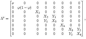
A. Structural Matrices for the Economy
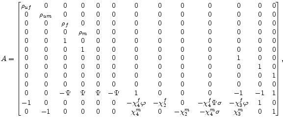
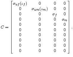
I represent the structural equations of the economy as

 ,
,
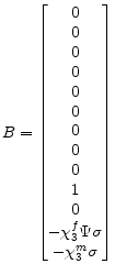 ,
,

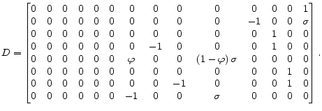
| (24) |
where
| |
||
 |
||
 |
and
![\displaystyle _{t}\left\{ \sum _{s=t}^{\infty}\alpha_{f}^{s-t}D_{t,s}\left[ P_{ft}\left( i\right) \left( 1+\tau_{f}\right) -V_{fs}\left( i\right) \right] y_{fs}^{d}\left( i\right) \right\}](img28.gif) ,
, ,
,![\displaystyle P_{ft}=\left[ \alpha_{f}P_{f,t-1}^{1-\theta_{ft}}+\left( 1-\alpha _{f}\right) \left( 1-\iota_{f}\right) \left( P_{ft}^{f}\right) ^{1-\theta_{ft}}+\left( 1-\alpha_{f}\right) \iota_{f}\left( P_{ft} ^{b}\right) ^{1-\theta_{ft}}\right] ^{1/\left( 1-\theta_{ft}\right) }](img50.gif) .
. ,
,