Polarization, immigration, education: What's behind the dramatic decline in youth employment?
Keywords: Youth employment, polarization, immigration, education
Abstract:
Since the beginning of the recent recession, the employment-population ratio for high-school age youth (16-17 years old) has fallen by nearly a third, to its lowest level ever. However, this recession has exacerbated a longer-run downward trend that actually began in the 1990s and accelerated in the early 2000s. There is little research regarding why teen employment has fallen. Some earlier work emphasized labor supply explanations related to schooling and education, such as an increased emphasis on college preparation (Aaronson, Park, and Sullivan 2006), while others have argued that adult immigrants have crowded out teens, at least in part because adult immigrants and native teens tend to be employed in similar occupations (Sum, Garrington, and Khatiwada 2006, Camarota and Jensenius 2010, Smith 2012). This paper presents updated trends in teen employment and participation across multiple demographic characteristics, and argues that, in addition to immigration, occupational polarization in the U.S. adult labor market has resulted in increased competition for jobs that teens traditionally hold. Testing various supply and demand explanations for the decline in employment since the mid-1980s, I find that demand factors can explain at least half of the decline unexplained by the business cycle, and that supply factors can explain much of the remaining decline.
1. Introduction
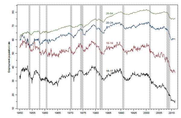
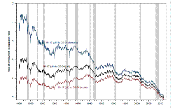
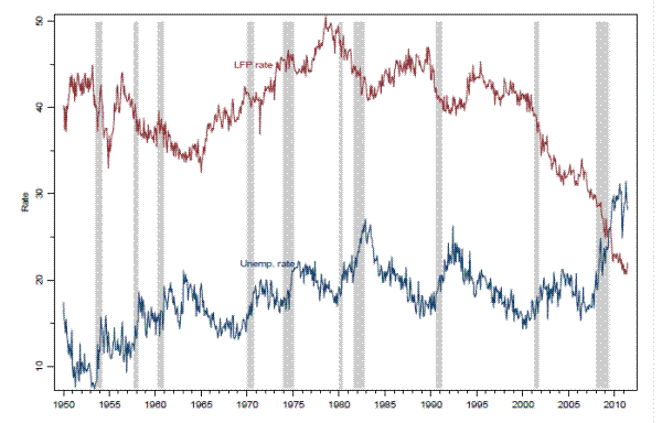
Since the start of the most recent recession, the employment-population rate for high school-age youth (16 and 17 year olds) has fallen from around 23 percent to around 15 percent, and is now at its lowest level since the Bureau of Labor Statistics began collecting data (figure 1).2 However, teen employment has been falling at about this rate since the early 2000s. Taking a longer perspective, youth employment rates have been trending down since the early 1980s; during every subsequent recession, the teen employment rate has tumbled and never recovered to its pre-recession level during the ensuing recovery. While employment rates have also fallen for slightly older, but not yet prime-aged adults, the decline is most dramatic for the youngest-which is particularly puzzling since the decline in employment for youth still in high school cannot directly be attributed to increased college enrollment rates. The decline in the teen employment-population rate looks even steeper relative to the employment-population rate for 25-54 year olds (the black line in figure 2). Figure 3 shows that, until recently, most of this decline was due to a drop in labor force participation rather than an increase in unemployment.
There is surprisingly little academic research related to understanding the causes of this decline in youth participation. Potential explanations naturally divide into supply and demand factors. Some possible supply factors are related to an increased emphasis on education, perhaps in part in response to a rising high school and college wage premium, which has increased the incentives to graduate high school, enter college, and attend a more elite college. Other education policy (such as stricter graduation requirements) may have also indirectly discouraged teens from working. Factors that may have reduced demand for teen labor include increased labor market competition from immigrants and native adults. Aaronson, Park, and Sullivan (2006), hereafter APS2006, provides one recent treatment of these issues; after demonstrating that the decline in youth employment is remarkably uniform across demographic groups, they provide ad-hoc tests for competing hypotheses. Their strongest finding is that teen employment rates fell more in states that provided merit-based college scholarships, perhaps because fewer teens needed to work in high school to save for college or because the returns to academic achievement in high school increased; they interpret this as suggestive evidence that supply explanations matter. On the other hand, recent research demonstrates areas that experience a larger increase in immigration have larger declines in teen employment (Sum, Garrington, and Khatiwada 2006; Camarota and Jensenius 2010; Smith 2012), suggesting that demand factors stemming from the increased supply of substitutable labor matter as well. Morisi (2008 and 2010) provide an excellent overview of trends in school year and summer employment, and carefully lays out hypotheses for the recent trends.
This paper has two purposes. First, it summarizes trends in teen employment in a manner similar to Morisi (2008 and 2010), and also introduces some new descriptive evidence from data sources such as the Survey of Income Participants (SIPP) and the American Time Use Survey (ATUS). Second, and more importantly, it takes another look at competing explanations for declines in youth employment over the last thirty years. Using evidence mainly from the cross-state or cross-commuting zone relationship between teen employment and supply and demand proxies over time, I conclude that labor demand explanations (stemming from increases in the supply of adult labor that is substitutable for teens) appears to explain more of the recent decline than do labor supply explanations (which are related to increased emphasis on schooling and college): The demand factors that I examine can explain between half to two-thirds of the decline in teen employment that is unexplainable by the cycle, and the supply factors I consider can explain most of the remaining fraction. Of course there are surely supply and demand factors that are not included in this analysis, but a conservative interpretation of this evidence is that both demand for teen labor and the supply of teen labor play an important role in explaining why fewer teens work than ever before.
Figure 4 provides an introductory overview of these arguments. It has been noted that the fraction of teens in the CPS who report being enrolled in school during summer months has been rising dramatically since the mid-1990s (Morisi 2010), which mirrors the downward trend in employment. Indeed, figure 4A shows that by July 2010, nearly half of 16 and 17 year olds report being enrolled in July. The blue line displays the fraction who report being enrolled in June, July, and August (using matched monthly CPS microdata); roughly one-third of teens now report being enrolled in school over the summer months. This may be due to increased attendance at formal summer school or informal academic and extracurricular camps, perhaps in order to appear more attractive to colleges; indeed, college enrollment rates (as calculated from CPS microdata) have continually risen over this period (figure 4B).
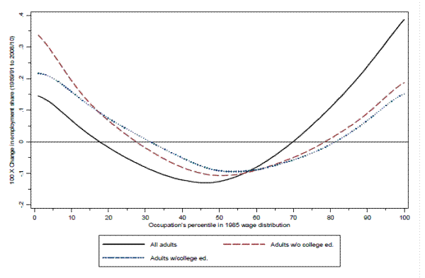
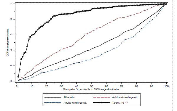
On the other hand, labor market competition from adults also appears to have been increasing: as shown in figure 4C, the immigrant share of the population has continually risen (and comparing the red and blue lines in figure 4D, immigrant adults are more likely than native adults to work in occupations that are common among teens). Further, the fraction of native adults working in teen jobs has also increased (figure 4D). This primarily reflects the increasing importance of the service sector as a source of adult employment, which in turn may be partially related to the polarization of the U.S. labor market (Autor and Dorn 2009). Figure 5 plots the smoothed change in the share of adults employed in every percentile of the occupational distribution (ranking occupations on the x-axis by their percentile in the 1985 wage distribution), and shows that share of adults in lower paying jobs has been increasing over the last few decades. Job polarization has been well-documented in the U.S. and other developed economies (Autor 2010; Goos, Manning, and Salomons 2009), and is hypothesized by some to be caused by declining computing costs, which have reduced the costs of mechanization and automation. As a result of this technological change (as well as possibly due to increasing ease of offshoring), some have argued that relative labor demand for easily routinized and mechanized occupations has fallen (which tend to be middle-paying jobs, such as manufacturing and clerical occupations), and as a result, some of the less-educated who were in (or would be in) those occupations have been displaced into lower-paying ones. Figure 6 shows that most employed teens work in these lower-paying jobs. Hence, it is possible that polarization of the adult labor market may increase competition in the labor market of which youth are a part. To date, the polarization literature mainly describes this structural change and tests explanations for it; to my knowledge, there is no research exploring the consequences of polarization on other populations that have not experienced as dramatic polarization in labor demand themselves, but which may nonetheless be affected by polarization of the labor market for prime-aged adults.
Although later sections in the paper test some of these hypotheses more carefully, figure 7 provides a flavor of the overall findings. States in which the fraction of teens enrolled in summer months increased more (a proxy for state attitudes towards education and state education policies) experienced somewhat larger declines in teen employment, although there is essentially no relationship between the change in teen employment-population and the change in the fraction of teens enrolled in summer months or the share attending college. Regarding potential labor demand explanations, there is a striking, negative relationship between the change in the share of the state that is immigrant and teen employment, and a negative but less significant relationship between the change in the share of native adults employed in teen jobs and the change in teen employment.
My primary finding is that, although youths' declining desire to work for educational reasons appear to be partially responsible for some of the fall in teen employment, a shift in labor demand (due to a rise in labor market competition from adults) also appears to explain much of the decline; in fact, the share of adults in teen jobs "explains" at least half of the total drop in youth employment unexplained by the cycle. A natural concern is that the number of employed teens and the number of adults in teen jobs are mechanically related and that cross-state relationships may be plagued by reverse causality. However, I provide a number of reasons to doubt this interpretation. First, even assuming that teen employment had not fallen (and assuming that adult displacement of teens is one-to-one), the share of adults in teen jobs would still have risen noticeably. Second, one theory of polarization suggests that the industrial and occupational mix of an area in a much earlier period is related to the degree of polarization that ultimately occurs. Using this idea, I isolate variation in the share of adults in teen jobs directly attributable to polarization with a Bartik-style (Bartik 1991) instrumental variable. If anything, the relationship between the share of adults in teen jobs and teen employment rates is larger in the IV specifications. Third, the share of adults in teen jobs is negatively related to the teen wage rate and positively related to the teen unemployment rate, consistent with this measure representing an exogenous decline in the demand for teen labor. Finally, the share variable itself is largely unrelated to the fraction of teens enrolled in summer months (a proxy for teen labor supply).
What are the eventual welfare consequences of permanently lower teen employment? As described in the next section, the existing literature provides mixed evidence on the benefits of employment in pre-graduation years, and it is beyond the scope of this paper to separately estimate the effects of youth employment on later life outcomes. However, I interpret the finding that demand factors matter as suggesting that not all of the decline in youth employment is "voluntary, " in the sense that it does not all stem from supply-related (academic) factors. With this interpretation, it is probably appropriate to be at least somewhat concerned about current levels of youth non-employment, especially for the non-college going segments of the population.
The next section provides additional motivation for studying the declines in teen employment and discusses the existing literature on the consequences of teen employment. Section 3 provides additional background on trends in employment across demographic groups, and presents data from the American Time Use Survey regarding what teens do if they are not working. Sections 4 and 5 explore supply and demand explanations more carefully, and section 6 pulls it all together by considering how much of the 30 year decline in teen employment may be attributable to supply and demand. Section 7 concludes.
2. Implications of declining youth employmentBefore delving deeper, it is worthwhile to consider why we should be concerned about lower teen employment rates. First, from a welfare perspective it is possible that work experience while school-aged has important benefits later in life, related to learning good work ethic, the importance of punctuality, the ability to deal with bosses and co-workers, and so on. However, the literature on the returns to working as a teenager on later life outcomes is surprisingly meager.3 The primary papers on the subject all use data from the National Longitudinal Survey of Youth 1979 to estimate the relationship between employment while in high school and later life labor market outcomes, controlling for the wide range of covariates made possible by the comprehensive nature of the NLSY. Ruhm (1997) finds positive effects of high school employment on earnings 5-10 years later, and Light (2001) finds that the returns to high school education are somewhat smaller after controlling for high school work experience (suggesting that work experience has positive effects on future earnings). More recently, Hotz et. al. (2002) argues that, after controlling for dynamic selection, work experience in high school has no effect, or possibly even a slightly negative effect, on future earnings. Although suggestive, these papers may have limited implications for recent declines in teen employment since the mid-1990s since they are derived from much older cohorts.
One reason for this may be that working part-time while in school detracts from other academic activities.4 There is a larger literature on this point, which is mostly in consensus that working while in high school has sizeable negative effects on academic achievement (Tyler 2003, though Rothstein 2007 finds smaller effects), though the effect may be non-linear with only the largest amounts of work having a deleterious effect on school grades (DeSimone 2006). The effect on grades may be more negative for minority high school students (Oettinger 1999), and working while in college also appears detrimental to grades (Arano and Parker 2008, Kalenkowski and Pabilonia 2010).
In summary, the literature provides inconclusive evidence on the degree to which employment while in high school is beneficial for human capital accumulation and future earnings, and therefore the welfare implications are similarly inconclusive. If teens are not working because of greater focus on graduating high school or improving their odds of college enrollment, then they may be substituting more formal forms of human capital acquisition for early work experience; given the wide college wage premium, this may have positive welfare consequences for college-bound teens. If instead teens are not working because adults are encroaching on their labor market, increasing competition in the lower-skill labor market and lowering wages (subject to the lower bound of the minimum wage), then this may be more detrimental (especially for non-college bound teens).5 Of course, increased competition in the lower-skill adult labor market may also encourage high school and college graduation by raising the returns to education, so over a longer period, a decline in demand for teen labor due to crowd-out may be indirectly associated with a shift in supply.
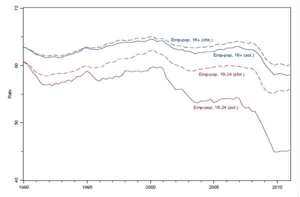
One other implication of declining youth labor force participation and employment is that it accounts for a disproportionate share of the recent declines in total participation and employment. Further, cohort-based models of U.S. labor force participation do a reasonably good job (at least until the mid-2000s) of explaining trends in participation for most groups, except teens (Aaronson, Fallick et. al. 2006); hence, understanding why teen employment is falling would improve the ability to forecast aggregate participation. To demonstrate the disproportionate importance of employment trends for youth, I first predict how the employment rate of 16-24 year olds would have evolved since 1990 had it responded to the business cycle (changes in the GDP gap) and changes in the adult employment-population rate as it had historically done.6 The red dotted line in Figure 8 shows this counterfactual. I aggregate this counterfactual rate with the actual employment-population rate for the 25 year olds (assuming that this rate evolved as it actually did) to get a counterfactual rate for the entire population. By the end of 2010, the counterfactual aggregate employment-population rate was about 2 percentage points above the actual, equivalent to about 40 percent of the actual decline since 1990 (for comparison, in 2010 16-24 year olds comprise about 16 percent of the population 16 and older).7
3. Looking further into youth employment and time useA. Some additional statistics regarding the trends in teen employment
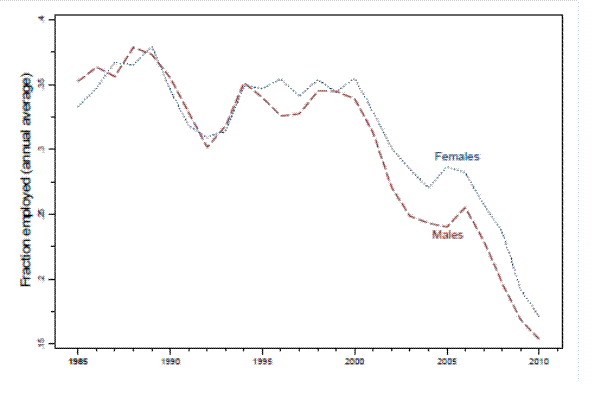
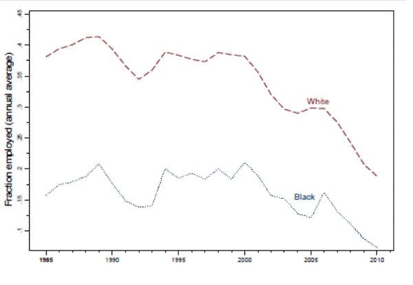
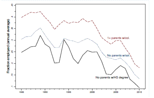
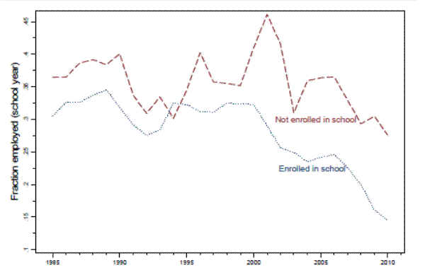
If the decline in youth employment is primarily due to an increased emphasis on academic activities (for improving the prospects of getting in to a better college), we might expect that employment rates fell more for groups that tend to have higher college attendance rates, such as females, whites, or teens from wealthier or better educated families. As shown in panels A, B, and C of figure 9, although employment rates are a bit higher for these groups on average, the decline is remarkably uniform (at least since the mid-1990s) across these groups. Additionally, it appears that employment rates may also have fallen for those not enrolled during the school year as well (panel D), although this series is admittedly noisy due to much smaller sample sizes (in 2010, about 95 percent of 16-17 year olds in the CPS report being enrolled during school year months).
Table 1 provides a range of summary statistics for hours worked (conditional and unconditional on being employed), the fraction employed and enrolled, and four mutually exclusive categories based on employment and enrollment status. On average in 1985, males worked more, while in 2010, this gender gap flipped and now females work more (columns 1 and 2). Conditional on employment (columns 3 and 4), however, male teens have always tended to work longer per week. Confirming figure 8, on average whites tend to work more than blacks, and teens with more educated parents also tend to work more; conditional on employment, the reverse tends to be true.
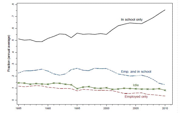
The next set of figures explores how other (very coarse) categories of time use have also changed. Figure 10 plots the (annual average) fraction of teens in each of four mutually exclusive categories: those who are only enrolled, employed and enrolled, only employed, and idle. Since the mid-1990s, there is a gradual decline in the annual fraction not in school (idle, and only employed), and somewhat more recently, a decline in the annual fraction both enrolled and employed. Thus, the fraction only in school has been rising, from about 50 percent in 1985 to over 70 percent in 2010. One important takeaway is that the fraction idle has not been rising despite a decline in employment rates; instead, there is evidently substitution (on an annual average basis) towards schooling.
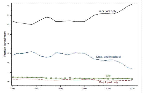
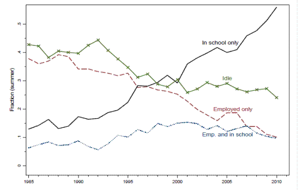
Looking at annual averages masks significant distinctions between summer and non-summer months. During school year months (figure 11), there is essentially a perfect inverse relationship between the fraction in school and the fraction employed and in school, suggesting that the decline in school year employment is coming almost entirely from a drop in the number of part-time working students. During summer months (figure 12), the story is different: summer employment rates have fallen evidently because the fraction only employed has fallen (the fraction in school and working actually increased over the 1990s and has since flattened out). The fraction in school only shows a surprising increase over much of the entire sample period, which I explore more carefully in the next section. Columns 9-16 of table 1 provide these statistics by demographic characteristics. During both the summer and school year months, the fraction idle is higher for blacks and for teens with less-educated parents, although the trends in all of these categories are fairly similar across all groups.
B. Time use among teens
What do teens do if they're not working? I use microdata from the American Time Use Survey to explore this question further. Table 2 shows the average number of hours spent per day on a variety of activities for employed and non-employed 15-17 year olds (I include 15 year olds to boost sample sizes); major activities within a column (education, employment, leisure, volunteering, personal care, household tasks, and other) sum to 24.
Is there any evidence that non-employed teens use their extra time for education-related activities? During the school year and school week, males who are working spend 1.7 hours more per week on employment-related activities (columns 1 and 2).8 The non-employed spend only 0.2 hour more per week on education-related activities, and all of this is coming from extra time spent on homework. In addition, they spend 1.2 more hours on leisure, the bulk of which is coming from games and computer usage, and an extra 0.7 hour for sleep (employed male teens spend more time on volunteering and other activities). For females, employed teens also spend 1.7 hours more per week on employment-related activities during the school year and school week. In stark contrast with males, non-employed females spend much of the extra time on education activities, (0.9 hour; 0.6 hour of this is from in-class time, 0.3 hour is from time spent on homework), with more modest differences for leisure time (0.4 more hours) and sleep (0.4 hours).
During the summer (weekday), employed males and females spend around 3 hours more per day on work-related activities than the non-employed (3.5 for males, 3.0 hours for females). For the non-employed (both males and females), only around 1 hour of this extra time is spent on educational activities. For males, the rest of the time is spent watching television, playing games or using the computer, or sleeping. For females, the rest is mainly spent watching television, sleeping, or helping with other household tasks.
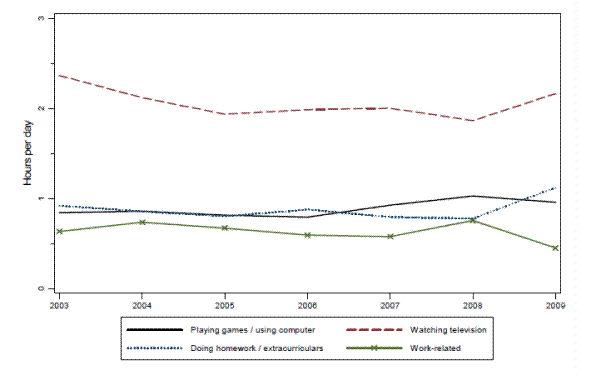
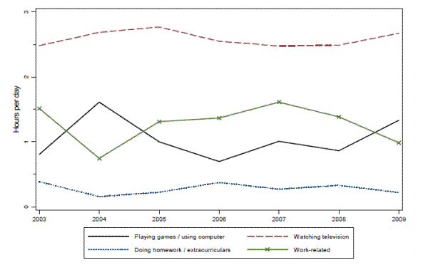
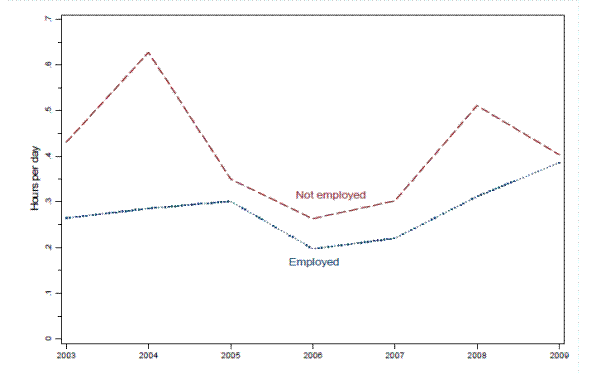
Figures 13 and 14 show trends in average time use on non-weekend days for school-year and summer months. Except between 2008 and 2009 there are no striking declines in the average amount of time spent in work-related activities, despite the decline in employment observed in aggregate CPS data. This is possibly because the data is noisy due to small sample sizes (on average, there are a bit more than 100 observations per year). Nevertheless, between 2008 and 2009-the first year of the recession-the decline in time spent on work-related activities appears to also be associated with an increase in time spent on homework and television watching during the school year, and associated with an increase in time spent watching television and playing games during the summer.
To sum up, although ATUS data is somewhat noisy due to small sample sizes, it appears that non-employed youth are spending some of their extra time on education-related activities, though clearly not most of it. At best (i.e. for female during the academic year), greater time spent on academics may account for 50 percent of the time not spent working; during summer months, and for males at all times, substitution towards academics is much less.
4. Exploring labor supply explanationsA. Documenting the rise in summer enrollment rates
As highlighted in the previous section, the share of teens who are enrolled in summer months has increased dramatically since the mid-1990s.9 It is important to explore the underlying causes of this trend in order to understand whether we should think of it as an exogenous supply shift in teen labor or possibly an endogenous supply response to rising returns to college in conjunction with declining demand for teen labor.
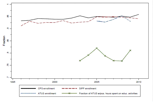
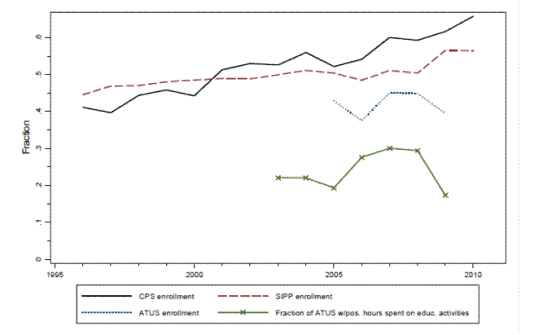
An increasing summer enrollment rate is not a unique feature of CPS data. Figure 15 shows that school-year enrollment rates are fairly similar in CPS, SIPP, and ATUS data (the school enrollment question is similarly phrased in each survey). Figure 16 shows that this is true in the summer as well; the fraction enrolled during summer months rises gradually in both the SIPP and CPS samples, and the estimated fraction is also quite high (above 30 percent) in the ATUS sample. Note that both during the school year and summer months, the fraction of ATUS respondents who report spending any time on education in the survey day is significantly lower. This is to be expected, since someone who is enrolled but absent on the survey day would appear as enrolled based on the enrollment variable but without having spent time on education that day.
B. Changes in state education policies as potential explanations for rising summer enrollment
What does the increase in summer school-going represent? One possibility is that teens now are more likely to be enrolled in formal courses in their local high school over the summer. This might be true if school years are starting earlier, more schools are moving towards year-round education, or if more states require students to pass exit exams to graduate (and those who fail receive remedial education over the summer). Alternatively, teens may be participating in greater numbers in less formal forms of summer education, such as academic, music, or sports camps, in order to improve their attractiveness to colleges, and may report being "enrolled" because they are participating in academic-style activities. Consistent with this, Ramey and Ramey (2009) show that the amount of time that parents spend on childcare increased dramatically beginning in the mid-1990s and increased more for better-educated parents. After ruling out other market-based explanations, they speculate that this is because parents are spending more time helping their children boost their attractiveness to colleges (i.e. driving their kids to music lessons, sporting events, and other extracurricular activities).
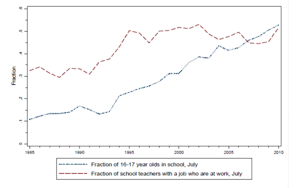
One piece of suggestive evidence that reported summer enrollment is related to subsequent college-going is that states with higher college attendance rates for their 19-21 year old population also have higher summer enrollment rates for teens.10 However, if the "college attractiveness" hypothesis explains all of the rise in summer enrollment, then it is unlikely that the number of primary teachers (i.e. elementary teachers) employed in the summer would increase substantially. CPS respondents are asked "what kind of work" they do regardless of current employment status, and, consistent with school teachers taking the summer off, a large fraction of those who report being teachers also report not being at work during the summer months; for instance, in summer 2010 nearly 50 percent of those who report themselves as teachers were not at work. However, the fraction of teachers at work in the summer increased from the early 1990s through the early 2000s, as shown by the red line in figure 17. Further, the shares of primary teachers at work in July show essentially the same pattern as that for secondary teachers (not shown). If the rise in teen summer enrollment is only because of tighter high school graduation requirements (a point which I explore more carefully below), then we might expect to see only the share of secondary teachers rise. Since the trend in July enrollment matches the trend in the share of teachers at work in July (at least through the early 2000s), it seems plausible that some of the increase in enrollment-and decline in employment-may be due to a change in the structure of the school year, i.e. more year-round schooling or a much earlier start date.
However, it does not appear that year-round education is widespread enough to be entirely responsible: For the 2006-2007 school year, the National Association of Year-Round Education estimates that about 2,750 public schools followed a year-round calendar, representing 2 million students, or
about 4 percent of total public enrollment (see also von Hippel 2007). It seems more likely that earlier start dates may explain some of the rise; Morisi (2010) cites evidence that about 75 percent of school districts now start teaching before September, up from 50 percent in 1988, and Market Data
Retrieval11 reports that around 20 percent of public schools will begin instruction prior to August 16![]() for the 2011-2012 school year.
for the 2011-2012 school year.
Another explanation is that more states require students to pass exams to graduate high school, and the difficulty of these exams (i.e. the grade level of the material it tests) has been increasing; students who fail the test the first time often attend summer school in preparation for taking it
again (Bishop and Mane 2001).12 For instance, my research into state laws (updating data from Dee and Jacob 2007) indicates that 27 states will require the
class of 2011-2012 to pass some sort of exam in high school in order to graduate, up from 14 in 1990. Of these, 3 states require "minimum competency" exams that test material at the 9![]() grade level or below, while the rest require more stringent tests. (Tests have evidently become more difficult over the years; in 1990, all states that required graduation exams only tested at the 9
grade level or below, while the rest require more stringent tests. (Tests have evidently become more difficult over the years; in 1990, all states that required graduation exams only tested at the 9![]() grade level or below.) In addition to exit exam requirements, the number of credits for high school graduation have also risen (Lillard and DeCicca 2001, Morisi 2010), which may induce students lacking in credits to attend summer school.
grade level or below.) In addition to exit exam requirements, the number of credits for high school graduation have also risen (Lillard and DeCicca 2001, Morisi 2010), which may induce students lacking in credits to attend summer school.
In addition to stricter graduation standards, one other relevant education policy is the introduction of merit scholarships for college. The most famous of these is the Hope Scholarship in Georgia, which in 1993 began provided full scholarships for in-state tuition for Georgia students with a B-average or higher in high school. Since then, an additional 10 states (mainly in the south) have enacted similar policies (see appendix table 1). APS2006 demonstrate that teen employment rates declined more over the first five years of the 2000s in states that provided merit scholarships than in other states. They suggest that this may be for two reasons. First, merit scholarships of these sorts increase the returns to high school achievement dramatically. Second, they also reduce teens' need to save for college and hence work in high school.
C. The relationship between education policy and teen enrollment rates
To estimate the association between these state education policy variables and teen employment and enrollment rates in the summer and school year months, I run OLS regressions of employment and enrollment rates (estimated from CPS monthly outgoing rotation group microdata) on a dummy for whether a state has an exit exam requirement that applies to current 16-17 year olds in year t, a dummy for whether the state has a merit aid scholarship program for college, and the number of credits in core subjects (English, social studies, math, science) needed to graduate (table 3). Year fixed effects are also included, as are state fixed effects for some specifications, and a host of controls as listed in the notes to the table. Because information is not available for all states in all years on the number of credits required for graduation, I first estimate the regressions without the credit requirement variable. The F-statistics for testing whether all three policy variables are equal to zero, and the associated p-value, are presented in the bottom of each panel.13
During summer months, states that require exit exams and more credits have higher summer enrollment rates and lower teen employment rates (columns 1 and 2, panels A and B), although the coefficient on exit exam is insignificant. On average, states that provide merit aid have summer enrollment rates that are around 5 percentage points higher, and summer employment rates that are 7 percentage points lower. A 1 credit increase in the number of required core credits (equal to about half of the average increase between 1990 and 2010 across all states) is associated with a 1 percentage point increase in summer enrollment and a 1 percentage point decrease in summer employment. However, after including state fixed effects (columns 3 and 4), the negative relationship between the state policy variables and summer employment becomes insignificant; this may be because there is something fundamentally different about states that enact stricter graduation requirements or provide merit aid (i.e. a weak within-state relationship), or because it takes the state teen population a few years to adapt and fully respond to these laws.14 States that provide merit aid for college also have lower teen employment rates during the school year (columns 5 and 6), consistent with the summer results; these are also insignificant after state fixed effects are added (columns 7 and 8). In general, these education policies are positively associated with log median wages (panel C), consistent with a shift in labor supply, though these results are rarely significant.
D. Are teens not working because family transfers have increased?
Household income per child may have been increasing for two reasons. First, median household incomes are higher now than in the early 1980s (though they have fallen from their peak in the late 1990s). Second, the average number of children (age 18 and under) has fallen somewhat since the early 1980s.15 As a result, median household income per child has risen about 20 percent over this period.16 A number of studies document a negative relationship transfers from parents to their children and their children's labor supply (Pabilonia 2001; Gong 2009; Dustmann, Micklewright and van Soest 2009), though these studies acknowledge that teen labor supply and cash transfers from their parents are likely endogenous.
As a first pass at exploring the relationship between the growth in household income per child and declining teen employment, I include an estimate of the log median household income per child (18 years and younger) for each state-year in the state-year level regressions that I ran in the above section. If anything, there is a positive relationship between the log of income per child and teen employment rates in the summer and school year17, though its causal interpretation is dubious because this relationship may reflect that states where incomes increased more had more strongly growing economies and may have had a greater relative increase in demand for youth labor as well. Without an independent instrument for household income, the causal link between rising household income and falling teen employment remains a topic open for further research.
E. Are teens not working because they're spending more times on video games?
One common assertion is that teens are spending more time watching video games and television than ever before. In fact, the fraction of 9![]() -12
-12![]() graders who used computers or played video games for three hours per day or more on an average school day increased from 22 percent to 25 percent between 2003 and 2009, though the fraction who watched television for
three hours per day or more fell from 38 percent to 33 percent.18 And, as shown in figures 13 and 14, based in ATUS data the average amount of time spent playing games is no more than an hour and has increased only modestly since 2003.
graders who used computers or played video games for three hours per day or more on an average school day increased from 22 percent to 25 percent between 2003 and 2009, though the fraction who watched television for
three hours per day or more fell from 38 percent to 33 percent.18 And, as shown in figures 13 and 14, based in ATUS data the average amount of time spent playing games is no more than an hour and has increased only modestly since 2003.
Of course, an increase in the amount of time that teens spend on using the computer or playing video games does not imply that teen labor supply has fallen because video game playing is more common. An equally plausible story is that employment has become more scarce, so teens have spent more of their time playing games and watching television, and this sort of substitution may be more easily accomplished now than decades ago because household income per child has risen. Nevertheless, it is possible that some of the increase in video game playing may represent a shift in labor supply. If true, then one possible exogenous supply shifter is the introduction of new gaming systems. The popularity of recent video game systems follows a natural cycle (Clements and Ohashi 2005). Once the system is first introduced, there are few available games and the system is priced above the systems from the previous generation. After a few years, the flow of new games increases, the system price generally comes down, the quality of games improves (as game designers learn how to squeeze the most out of each system's processing capabilities), and sales accelerate. Towards the end of a system's lifecycle, interest diminishes as the graphics and performance quality of games plateau and gamers look forward to the introduction of the next generation of systems.
Consistent with this hypothesis, as shown in figure 18, the average amount of time spent on video games declined from 2005 to 2006 as the previous generation of systems neared the end of their cycles and new systems were announced (Sony Playstation 2, released in the U.S. in 2000; Nintendo Gamecube and Microsoft Xbox, which were released in the U.S. in at the end of 2001).19 Game usage then picked up as the next round of systems were released in the subsequent years (end of 2005 for the Microsoft Xbox 360; end of 2006 for the Nintendo Wii and Sony Playstation 3). Although this pattern is suggestive evidence that the availability of videogames itself can influence time usage, the difference in videogame usage between employed and not employed males is too small to account for the difference in time spent on work-related activities. For instance, for 15-17 year old males, the non-employed play about 25 more minutes of games per school day than the employed, about 30 percent of the difference in time spent on work-related activities.
F. Summary
To conclude this section on labor supply, there is ample evidence that time spent on academic activities is increasing, especially in the summer months. It is likely that this is at least in part because graduation requirements have gotten stricter, and because a growing number of states now provide tuition subsidies to in-state colleges for accomplished high school students-and there is suggestive evidence that these education policies may directly reduce the labor supply of teenagers. Rising household income per child also remains a potential labor supply related explanation that requires additional research.
5. Exploring labor demand explanationsA. Decomposing growth in the share of adults in teen jobs
As explained in section 1, the occupational distribution of the U.S. adult labor market has "polarized," with relative wages and employment growing for the highest and lowest paying occupations. The prevailing explanation is that declining costs of computerization and automation have reduced labor demand for jobs that specialize in routinized tasks (such as clerical and manufacturing labor, which were historically middle-paying, "middle-skill" jobs), increased labor demand for jobs that are made more productive by this technology (jobs that require abstract, creative, design-based tasks, i.e. jobs requiring more education), and have had little direct effect on labor demand for jobs that require manual tasks (which are not routine and not easily automated, i.e. service sector jobs). One implication of the decline in labor demand for middle-skill jobs is that the people who were in these occupations, or future workers who would have been in them eventually, may be displaced to lower-skill, lower-paying service sector jobs. As argued in section 1, these jobs are the ones most commonly held by teens.
The bottom of table 4 shows that the percent of all adults (regardless of education, gender, or native status) in what I classify as teen jobs increased from 23.7 percent in 1995 to 24.4 percent in 2010.20 The number of adults in teen jobs increased from around 27.5 million to 32.3 million, an increase of over 5 million, whereas the number of employed 16-17 year olds fell by nearly 1 million.21 The modest increase in the overall share of adults employed in teen jobs masks important increases within education, gender, and nativity cells. For instance, the share of native adult males without a college education in teen jobs increased by 3.5 percentage points over this period. However, the aggregate share of all adults in teen jobs increased by less than this amount because the employment-to-population ratio for non-college adults fell (column 2), as did their population share (column 3). To assess the contribution of each group to the rise in the aggregate share of adults in teen jobs, I carry out the following calculation for each education/gender/nativity group j:

From this exercise, it is clear that more than the entire increase in the share of all adults in teen jobs is attributable to an increase in immigration (i.e. the change in the Cs for immigrants, the first two panels of column 4, sum to 2.3), as a greater share of immigrants work in teen jobs and their population share increased dramatically over the 15 year period. Although the share of natives in teen jobs has increased over this period, the composition of the native population shifted from less- to more-educated, thus (in an accounting sense) offsetting the upward influence of immigration on the aggregate share. In other words, the share of native adults in teen jobs has been increasing more within education classes than in the aggregate, while the composition of the native population has been shifting towards groups that are less likely to work in teen jobs. Nonetheless, even though the population share and employment rates of non-college native adults fell over this period, had the share employed in teen jobs not increased as it did, then the aggregate share in teen jobs would likely not have increased as much; hence, the movement of less-educated adults into teen jobs may still be a significant explanation for why teens are less likely to work.
B. Estimation strategy
Next, I turn to my primary findings, which are estimates of the relationship between the share of adults in teen jobs (or in lower-paying jobs, or in service sector jobs) and teen employment. The share of all adults in teen jobs may be viewed as a proxy for increasing labor market competition from a number of sources, including growth in the number of low-skilled immigrants, polarization of the adult labor market for natives, increasing labor force participation for those near retirement age, and increasing labor force participation for less-educated, single mothers (due to welfare reform or the EITC).22 I show this more directly in table 5. This table displays regression coefficients from state-year level regressions of the share of all employed adults in teen jobs (or all employed adults without college education, in columns 5 and 6) on the covariates listed in the table as well as state and year fixed effects. As shown in column 1, the aggregate share is positively related to the share of non-college and college adults in teen jobs. Somewhat surprisingly, the results in columns 2 and 3 suggest that, if anything, the employment rate for those post-retirement age is negatively related to the overall share of adults in teen jobs. These results also demonstrate that immigration is not the only thing pushing up the aggregate share (the share of native adults in teen jobs remains strongly related to the aggregate share after controlling for immigration).
I view the OLS relationship between teen employment and the share of adults in teen jobs, after controlling for state and year fixed effects and the controls listed at the bottom of table 7, as probably capturing much of the causal impact of adult crowd-out. There are a number of natural concerns to this interpretation. One is reverse causality, that is, if teen labor supply declined exogenously, then there would be increased demand for adult workers for teen jobs. I address this concern in a number of ways. First, the decline in teen employment is only a small fraction of the increase in the number of adults in teen jobs, suggesting that the importance of reverse causality is likely minimal.23 Second, I use a Bartik (1991) style instrument to isolate the variation in the share that is driven by national trends in polarization interacted with the state's scope for polarization in 1980; if anything, the 2SLS relationship between teen employment and the adult share in teen jobs is more negative (though less precise). Third, I show that the adult share variable is negatively related to teen wages and positively related to teen unemployment, consistent with this relationship capturing the effects of a shift in demand for teen labor. Finally, I also show that the share of adults in teen jobs is largely unrelated to shifters of teen labor supply that are related to education.
Another concern is that there may be other state-specific shocks that both increase the number of adults in these jobs while directly reducing the number of employed teens. In fact, most plausible biases imply that the true causal effects are more negative than OLS estimates suggest. For instance, if immigrants tend to settle in areas with more favorable labor markets, then this type of endogenous immigration would bias OLS towards less negative effects. Similarly, , if less-educated adults tend to move out of labor markets that become more polarized, then the true causal effects of polarization on teen employment would be more negative than the OLS relationship suggests.24
To further address this and other endogeneity concerns, my primary specification uses an IV-strategy to directly instrument for the share of adults in teen jobs, based on the share of adults in teen jobs in the state in 1985 interacted with the average share across all states in each year. The motivation behind this instrument comes from a recent paper by Autor and Dorn (2009), which provides a structural model of polarization.25 The model predicts areas that most heavily utilized routinized labor prior to the acceleration in polarization in the 1980s and 1990s (i.e. areas that employed a greater share of workers in occupations that specialize in routine tasks, like manufacturing and clerical work) have the most scope for polarization, will respond most strongly to improving automation and declining computer costs, and will therefore have shown the most polarization over time. Hence, if cross-state differences in the share of adults in teen jobs reflect underlying polarization, rather than the endogenous response to shifts in teen labor supply, then labor markets should have polarized more-and teen employment should also have fallen more-in labor markets for which routinized tasks were more important in the production process.
Table 6 verifies this using microdata from the Census and American Community Survey. The dependent variable in panel A is the change in the fraction of native adults in teen jobs (between 1980 and 2007). The two covariates of interest are the degree to which routine tasks are used in the state (or commuting zone) in 198026, and the share of adults in production occupations in 1980.27 The theory outlined above suggests that areas for which occupations specializing in routine tasks were more prevalent in 1980 should have experienced greater subsequent increases in polarization; partially, though not entirely, this is because areas that with more "routinized occupations" were also more heavily specialized in manufacturing and production. Indeed, there is a strongly positive relationship between the routine task intensiveness of an area in 1980 or the share of adults in production occupations in 1980 and subsequent polarization. This relationship remains reasonably strong whether these summary statistics for the 1980 occupational distribution are entered separately or together, and whether the analysis is done at the state or commuting zone level.28 Consistent with adults crowding out teens, teen employment (panel B) also fell more in areas that were more heavily routinized in 1980 (though not for areas that concentrated in production occupations).
These findings suggest using a Bartik-style (Bartik 1991) instrumental variable, which I construct by interacting the share of adults in teen jobs in 1985 (the start of the analysis) with a national summary measure of the share of adults in teen jobs (I use the unweighted average share across states in each year). This instrument isolates variation in the share of adults in teen jobs that comes from polarization of the adult labor market, rather than the reverse channel of falling teen employment or endogenous immigration. The relationship between the share of adults in teen jobs in a year and this instrument is very strong and negative, that is, areas that had a larger share of adult in teen jobs in 1985 experienced smaller increases in the share over the next 30 years (from a first-stage regression of the share of adults in teen jobs on this instrument, state and year fixed effects, and the host of controls listed in the bottom of table 2, the coefficient on the instrumental variable is -18.3 and the standard error is 2.4).
C. Estimates of the impact of increases in the share of adults in teen jobs on teen employment
The first column of table 7 shows the coefficient from a regression of teen employment rates on the share of employed adults without college experience, controlling for state and year fixed effects and a host of other controls (as indicated in the note to the table). The dependent variable and the share variable are calculated each as fractions, so the interpretation of the coefficient in column 1 is that a one percentage point increase in the share of non-college adults in teen jobs is associated with a 0.4 percentage point decrease in teen employment rates. In column 2, I instrument the share variable with the share in 1985 for each state interacted with the national average share in each year. The coefficient, though less precise, is larger in magnitude, suggesting that reverse causality is not driving the relationship (and in fact the other forms of endogeneity discussed above, such as immigrant locational choice and native out-migration may negatively bias the OLS results).
In columns 3 and 4, the share variable is estimated over the entire adult population (unconditional on education). Although the coefficient is larger in magnitude, the change in the share over the sample is smaller, and the overall "impact" of polarization on teen employment over this period (the product of the coefficient and the actual change) is also somewhat smaller. In columns 5 and 6, share is defined as the share of non-college adults in lower paying jobs (jobs in the bottom quarter of the wage distribution in 1985), and in columns 7 and 8, the share is defined as the share of adults in retail or service jobs. These are all analogous methods of describing the impact of polarization on the lower tail of the occupational skill-distribution, and all are negatively (and significantly) associated with teen employment; as before, IV estimates are larger in magnitude, though in some cases, very imprecise.29 Finally, in columns 9 and 10, the share variable is defined as the share of adults in production or office jobs, which tend to be in the middle of the skill or wage distribution, and which lost employment share over these periods (i.e. the "hollowing out" of the middle, as seen in figure 5). An increase in this share is associated with an increase in teen employment, consistent with the notion of a negative relationship between the share of adults in these jobs and the share in service, retail, lower paying, or teen jobs. Given the magnitude of these coefficients and the change in the share between 1985 and 2010, and giving preference to the IV estimates, these results imply that polarization in the adult labor market can explain between 1 percentage point (column 4) to 9 percentage points (column 6) of the 18 percentage point decline in youth employment over this period. I more carefully estimate counterfactual changes in teen employment in the final section of this paper.
The rest of the table presents estimates from additional robustness checks. In column 11, I include state time trends. The coefficient is somewhat larger in magnitude than the baseline, though here the relationship is extremely imprecise. In column 12, I limit the time period to 1995-2009 and the relationship is in fact much stronger than baseline (although again, imprecise). In column 13, I limit calculation of the share variable to the native population, and the implied impact is somewhat smaller (which is to be expected, since available evidence suggests that immigration negatively affects teen employment and, as shown earlier, is responsible for part of the increase in the share of adults in teen jobs). Finally, in column 14 I also include the employment rate for adults, and this has almost no effect on the magnitude of the coefficient for the share of adults in teen jobs, suggesting that negative labor market shocks (correlated with changes in relative labor demand across skill-type of job) are not driving these findings.
Table 8 estimates the same sort of regressions with the teen log median hourly wage as the dependent variable. The coefficient on the share variable is always of the same sign as in the previous table (positive in columns 9 and 10, and negative in the others) albeit often imprecisely estimated, suggesting that an increase in the share of adults in teen jobs indeed represents a decline in demand for teen.
In table 9, I take concerns about the endogeneity of immigrant concentrations more seriously. The share variable in the regressions presented in this table is estimated only for native adults, and is estimated from Census data for 1980, 1990, and 2000, and American Community Survey data for 2009. These regressions are differenced versions of those presented in earlier tables, with similar controls, except that state fixed effects are not included (because the results are differenced). The share of the non-college population that is immigrant also enters as a separate variable. I use a differenced equation because, as discussed in Smith (2012), the IV strategy as defined below predicts changes in immigrant concentrations.
In column 1, teen employment rates (the dependent variable) are estimated from CPS data. The share of native adults in teen jobs is negatively associated with teen employment, although not significantly so. In column 2, I instrument for immigrant shares using two instruments. One is based on the idea that immigrants of a certain ethnicity tend to settle in areas where that ethnicity has settled in the past, regardless of current labor market conditions. The second is based on a state's distance to Mexico, interacted with national trends in the immigration of Mexicans, since Mexican immigrants tend to settle closer to the border, regardless of current labor market conditions. Further detail on the construction of these instruments is provided in Smith (2012).30
After instrumenting for immigrant shares (column 2), the coefficient on immigrant share becomes negative, suggesting that selective immigration into areas with more positive labor market conditions may bias OLS coefficients towards zero. However, estimates are still imprecise. One possibility is that, due to small sample sizes in the CPS data, state-level estimates of employment rates are noisy, and differencing over time exacerbates this. I therefore move to estimating employment using Census and ACS microdata. Column 3 demonstrates that, after doing so, both the share of native adults in teen jobs and the immigrant share of the population are strongly negatively associated with teen employment rates. In column 4, I add an instrument for adult natives in teen jobs, motivated from the earlier analysis (interacting the share of native adults in teen jobs in 1980 with the average change in the share, across states, between 1980 and 1990, 1990 and 2000, and 2000 and 2009). This has no effect on estimates of the immigration effect, but boosts the measured impact of the share of adult natives in teen jobs (though it is now much less precise).
In columns 5 and 6, I estimate similar differenced regressions, except that the unit of analysis is a commuting zone rather than a state. These results also support the strongly negative association between the share of adults in teen jobs and immigrant shares, and teen employment, and reinforce that the relationship between the share of adults in teen jobs and teen employment as estimated in table 7 is not entirely because areas with greater immigrant concentrations will mechanically have a greater share of adults in teen jobs.
In summary, estimates from this section suggest that there is a strongly negative relationship between the share of adults in teen jobs, that this relationship is robust to the choice of time period and how the share variable is measured, and that this relationship appears as if it may be causal in nature. Based on estimates from table 7, anywhere between 1 to 9 percentage points of the 18 percentage point decline in teen employment rates between 1985 and 2010 may be explainable by these measures of adult employment in teen or lower-paying jobs. However, these estimates do not simultaneously control for supply measures; the next section puts all of the pieces together to consider the relative importance of both supply and demand in explaining recent movements in youth employment.
6. Putting it together: demand, supply, or both?
The analysis in sections 4 and 5 demonstrate that both supply (schooling decisions and state education policy) and demand (the supply of adults to teen jobs) appear to be driving much of the observed decline in youth employment. This section concludes by considering the degree to which each is responsible.
To begin, table 10 estimates OLS and 2SLS regressions of teen labor market outcomes (estimated during the school year) on the fraction of adults in teen jobs (instrumented as described in section 5), the fraction of teens who report being enrolled in June, July, and August using matched CPS data (a proxy for labor supply), the fraction of 19-21 year olds in college (a proxy for a state's intensity of college attendance and hence also a proxy for teen labor supply), whether the state provides merit aid scholarships (a policy variable that should influence supply, based the findings from section 4), the log of the minimum wage, state and year fixed effects, and other controls listed in the bottom of the table.
Turning first to the demand variable, an increase in the share of adults in teen jobs is negatively associated with teen employment, participation, and log median wages (note that the OLS relationship is significant, while the 2SLS coefficient is generally larger in magnitude but often very imprecise). It is positively associated with the unemployment rate in the OLS specification (again, 2SLS estimates are very imprecise). Finally, there is no strong evidence that more adults are working in teen jobs in areas where teen employment is lower for labor supply reasons: there is only a weak (albeit positive) relationship between the share of adults in teen jobs and the fraction of teens enrolled in all summer months (columns 11 and 12). This, along with the negative relationship between the share variable and teen wages, and the positive relationship between the share variable and the teen unemployment rate, is further suggestive evidence that the negative correlation between adult employment in teen jobs and teen employment is due to adults crowding out teens, rather than because an exogenous decline in teen supply draws adults into the market. Regarding the variables that proxy for labor supply, they are generally negatively associated with teen employment outcomes, although never statistically different from zero.
Table 11 estimates employment effects for various sub-groups of the teen population, separating teens by gender, race, parental education, and whether the teen reports being enrolled during the school year or not. Due to smaller sample sizes, the results for many cells are imprecise. Nevertheless, a few consistent findings stand out. First, the labor demand variable is negatively associated with employment for almost all groups, and the magnitude is greater for females and for those from families with less education. Second, supply measures are also negatively associated with teen employment rates; the coefficients are of roughly the same magnitude for all groups, though rarely are these estimates significant and they are never precise enough to be statistically different from each other. On the whole, these estimates suggest that supply and demand factors appear to jointly affect teen employment, and that the decline in labor demand for teens might have even greater effects on employment for the most at risk populations such as those with less-educated parents.
APS2006 show that teen employment rates fell over the 2000s more for states that provided merit aid scholarships. One interpretation of this is that there is an interaction between trends in labor demand (either cyclic or more persistent) and the ability and desire for teens to substitute time towards schooling; that is, if competition in the teen labor market increases, as it did over the 2000s, teens may be more likely to drop out of the labor force if the opportunity costs to working are greater and if the substitutes for their time (i.e. academic activities) are more attractive. To assess this further, I first estimate a time trend for teen employment in each state between 2000 and 2010. I then regress this time trend on four state characteristics, measured in 2000. To proxy for the state of labor demand for teens in 2000, I include the share of adults in teen jobs and the immigrant share of the population. To proxy for the attractiveness of academic pursuits and the willingness of the state's youth population to focus on academics, I include the fraction of teens enrolled in school during the school year (in 2000). Following APS I include the merit aid dummy as well. Column 1 includes only demand measures; teen employment actually fell less for states in which more adults were employed in teen jobs in 2000. This is consistent with the earlier findings from table 6 that showed polarization tends to be greater in areas that begin as less polarized. Column 2 includes only supply measures, and teen employment rates fell much more in areas that had higher enrollment rates or offered merit aid scholarships in 2000. Column 3 includes all measures, and the magnitude and statistical significance of the coefficients remain largely unchanged. In sum, the results from this table present suggestive evidence that declines in demand (from polarization and the cyclical relative declines in demand for teen labor due to the weak labor markets in the 2000s) may interact with state education policies that affect youths' willingness to substitute time away from work and towards academics.
Supply and demand both evidently matter for explaining much of the decline in youth employment. But how much of the decline can be attributed to each? To address this, I construct counterfactual teen employment and participation rates, holding supply and/or demand factors at their 1985 level. To begin, I again estimate a state-year level 2SLS regression of the teen employment rate (this time, using annual averages) on the log minimum wage, the share of non-college adults in teen jobs (demand factor), and the following supply factors: the fraction of teens enrolled in the summer, the fraction of teens enrolled in the school year, the college enrollment rate for 19-21 year olds two years later, and whether the state offers merit aid scholarships or requires an exit exam.31 To form a counterfactual estimate of the teen employment rate had supply or demand factors not changed over the last 25 years, I hold these factors at their 1985 level and use the estimated coefficients from the regression to adjust each state's teen employment or participation rate to this counterfactual level. I then aggregate to the national level to form counterfactual rates holding either supply factors, demand factors, or both fixed at 1985 levels. For this exercise to be meaningful, I also compute a baseline counterfactual employment rate, which is the predicted teen employment or participation rate if it were to respond to the cycle (the CBO's estimate of the GDP gap) and the employment-population ratio for prime-age for adults in its "historical manner."32
Table 13 (employment rates) and table 14 (participation rates) display the results of this exercise. The first line in the top panel shows the actual change in the (annual average) employment or participation rate between 1985 and 2010. The second line shows the projected change had changes to the rate responded to changes in the GDP gap and changes in adult employment (or participation) rates in its usual fashion. Hence, the amount "explained" by the cycle (the combination of movements in the GDP gap and adult employment or participation) is the decline predicted in the second line. The goal of this exercise is to see how much of the remaining decline can be explained by the supply and demand factors considered previously.33 Changes in the GDP gap and the adult employment (or participation) rate can explain 60 percent of the decline in teen employment and 50 percent of the decline in teen participation (the third column of line 2).
The third, fourth, and fifth lines of the table adjust for supply and demand factors (and the minimum wage), independently, as well as in concert. Supply factors matter: Holding the supply factors (summer enrollment rates for 16-17 year olds, exit exams, merit aid scholarships, college enrollment rates) at their 1985 level, teen employment would have fallen 17 percentage points, and so supply factors can "explain" an additional 1 percentage point of the total decline or 6 percent of the total decline (or about 16 percent of the decline not explained by the cycle, column 4). Similarly, supply factors can explain an additional 3 percentage points of the decline in participation (35 percent of the remaining decline). In contrast, the teen employment rate would be about 4 percentage points higher if the demand for teen labor remained at its 1985 level, and the participation rate would be about 2 percentage points higher. In total, these supply and demand factors (and the minimum wage) can "explain" most of the decline in the teen employment and participation rates that is unexplained by the cycle variables (80 percent of the remaining decline in teen employment, 75 percent of the remaining decline in teen participation).
The next panels of each table explore the robustness of these findings to the inclusion of some additional variables. To control for other factors that may influence encourage teens to focus on education, in panel B I also include returns to college, estimated as the difference between log median earnings for college graduates and non-college graduates in the state/year. It is debatable whether this should count as a supply or demand factor; assuming that it is unrelated to polarization and the rise in the share of adults in teen jobs, and that it proxies for other omitted variables related to benefits from education, then it may reasonably be included as a factor affecting labor supply. However, to the extent that polarization increases the college premium and also pushes some less-educated adults into teen jobs, counting this factor as a supply-related variable will overestimate the contributions of supply and underestimate the contributions of demand. Nevertheless, I include it in this analysis to be as complete as possible, and tentatively classify it as a supply factor, recognizing that its inclusion and classification may be disputable.
Focusing first on employment rate counterfactuals, including this measure of returns to education as a supply factor raises the contribution of supply factors to about 17 percent of the total decline in teen employment (or 43 percent of the unexplained decline), and lowers the contribution of demand factors slightly. However, once state time trends are included in the regressions, the contribution of supply factors is reduced back to the baseline, and the contribution of demand factors increases; in this specification, supply factors and demand factors respectively explain around 17 percent and 70 percent of the decline unexplained by the cycle.
Turning back to participation in table 14, including returns to education as a supply variable (panel B) raises the contribution of supply factors substantially and lowers the contribution of demand factors somewhat; now, supply factors explain 22.5 percent of the total decline or 60 percent of the decline unexplained by the cycle, while the demand factor explains less than 10 percent of the total decline, or just over 20 percent of the unexplained decline. Again, including state time trends (panel C) reduces the contribution of supply and boosts the contribution of demand; in this specification, supply and demand factors explain around 30 percent and 60 percent of the unexplained decline in teen participation, respectively.
To summarize the findings of this exercise, both supply and demand factors evidently matter in explaining why teen employment and participation rates have fallen. However, across most specifications (except for labor force participation in panel B), the labor demand factor explains at least as much as the supply factors do, and in some specifications, labor demand explains a lot more. Of course, the outcome of this exercise is also dependent on what proxies for labor demand and supply are included; to the extent that key proxies for labor supply or demand are missing, these estimates are potentially underestimates of the true contributions of each factor.34
7. Conclusion
Employment rates for high school age youth has fallen nearly 20 percentage points over the last 25 years. Over this period, the share of adults employed in teen jobs has risen due to various reasons, including immigration and polarization in the adult labor market. At the same time, the share of teens involved in educational activities over the summer and enrolled during the school year has risen, likely reflecting the rising returns to college, as well as state education policies (stricter graduation requirements, merit aid scholarships) and possibly also reflecting an endogenous response to increasing labor market competition.
This paper represents the latest and most comprehensive attempt to address these factors in combination. Based on the proxies for labor demand and supply included in this analysis, teen employment rates would be at least 3½ percentage points higher in 2010 (and up to 5 percentage points higher, depending on the specification) if not for declining labor demand due to increasing competition in the low-skilled labor market (i.e. crowd out by adults). Labor supply explanations can each explain at most another 3 percentage points or so of the decline in teen employment (the contribution of supply factors are somewhat more significant for counterfactual estimates of labor force participation rates). Much of the crowd-out from adults is likely due to polarization of the adult labor market, driven by the declining costs of computerization and automation which have displaced some less-educated adult workers into service sector jobs that teens tend to do. This finding is the first evidence, to my knowledge, regarding how occupational polarization in the labor market for prime-age adults also indirectly affects other labor markets. Related questions for future research include how this trend in low-skill adult employment has affected employment outcomes and occupational choice for other traditional participants in the lower-skill, service-sector labor markets (i.e. immigrants, natives near retirement age).
One interpretation of these findings is that the decline in teen employment has potentially troubling long-term consequences, since a significant fraction of it appears due to shifts in labor demand. Nevertheless, it appears that teens are substituting more formal forms of human capital (i.e. summer school and college prep) for work experience, which may mitigate some of the negative effects. This is especially true if teens were previously spending inefficiently low amounts of time on academics. Although analyses of time use data, like the one presented here, start to fill in our knowledge about what non-employed teens are doing with their extra time, bringing additional data to bear on the question, with longer sample periods and larger samples, will be valuable for describing what non-employed teens are doing with their time, how time use has changed over the years, and ultimately what the long-run ramifications may be. At the moment, we do not know enough about the returns to working while in high school (relative to the returns to alternative time uses) to make definite conclusions about welfare costs; future research might address this question by using the supply and demand shifters presented in this paper to explore how youth non-employment affects later life outcomes. At a minimum, these results are strongly suggestive that the on-going decline in teen employment is at least not entirely due to a shift in labor supply.
Table 1a: Summary statistics by demographic characteristics: School year months
| Avg. hrs / week (uncond.): 1985 (1) | Avg. hrs / week (uncond.):2010 (2) | Avg. hrs / week (cond. on working): 1985 (3) | Avg. hrs / week (cond. on working): 2010 (4) | Fraction employed: 1985 (5) | Fraction employed:2010 (6) | Fraction enrolled: 1985 (7) | Fraction enrolled: 2010 (8) | Fraction only in school: 1985 (9) | Fraction only in school: 2010 (10) | Fraction employed and in school: 1985 (11) | Fraction employed and in school:2010 (12) | Fraction only employed: 1985 (13) | Fraction only employed: 2010 (14) | Fraction idle: 1985 (15) | Fraction idle: 2010 (16) | |
|---|---|---|---|---|---|---|---|---|---|---|---|---|---|---|---|---|
| All | 5.2 | 2.2 | 17.1 | 15.6 | 0.31 | 0.15 | 0.92 | 0.96 | 0.64 | 0.82 | 0.28 | 0.14 | 0.03 | 0.01 | 0.05 | 0.03 |
| Males | 5.6 | 2.2 | 17.8 | 16.2 | 0.32 | 0.14 | 0.92 | 0.95 | 0.64 | 0.83 | 0.28 | 0.13 | 0.03 | 0.01 | 0.05 | 0.03 |
| Females | 4.8 | 2.3 | 16.4 | 15.0 | 0.30 | 0.16 | 0.92 | 0.96 | 0.64 | 0.81 | 0.28 | 0.15 | 0.02 | 0.01 | 0.05 | 0.03 |
| White | 5.8 | 2.5 | 17.2 | 15.3 | 0.35 | 0.18 | 0.92 | 0.96 | 0.60 | 0.80 | 0.32 | 0.16 | 0.03 | 0.01 | 0.05 | 0.03 |
| Black | 2.2 | 1.2 | 17.3 | 19.0 | 0.13 | 0.06 | 0.93 | 0.95 | 0.82 | 0.90 | 0.11 | 0.06 | 0.01 | 0.01 | 0.06 | 0.04 |
| At least one parent with college ed. | 5.6 | 2.3 | 15.7 | 14.4 | 0.37 | 0.17 | 0.96 | 0.97 | 0.61 | 0.81 | 0.35 | 0.16 | 0.02 | 0.01 | 0.02 | 0.02 |
| No parents with college ed. | 4.8 | 2.0 | 17.9 | 17.4 | 0.27 | 0.12 | 0.91 | 0.94 | 0.67 | 0.84 | 0.24 | 0.10 | 0.03 | 0.02 | 0.06 | 0.04 |
| No parents with a high school degree | 3.8 | 1.6 | 17.5 | 19.8 | 0.22 | 0.08 | 0.88 | 0.93 | 0.69 | 0.86 | 0.19 | 0.07 | 0.03 | 0.01 | 0.09 | 0.06 |
| Enrolled in school | 4.7 | 2.0 | 15.7 | 14.5 | 0.31 | 0.15 | 1.00 | 1.00 | 0.69 | 0.85 | 0.31 | 0.15 | 0.00 | 0.00 | 0.00 | 0.00 |
| Not enrolled in school | 11.2 | 7.4 | 30.9 | 28.7 | 0.36 | 0.28 | 0.00 | 0.00 | 0.00 | 0.00 | 0.00 | 0.00 | 0.36 | 0.28 | 0.64 | 0.72 |
Source: Authors' calculations from CPS monthly outgoing rotation group microdata. Sample is for 16 and 17 year olds. School year months are January-April and October-December. Summer months are June-August.
Table 1b: Summary statistics by demographic characteristics: Summer months
| Avg. hrs / week (uncond.): 1985 (1) | Avg. hrs / week (uncond.):2010 (2) | Avg. hrs / week (cond. on working): 1985 (3) | Avg. hrs / week (cond. on working): 2010 (4) | Fraction employed: 1985 (5) | Fraction employed:2010 (6) | Fraction enrolled: 1985 (7) | Fraction enrolled: 2010 (8) | Fraction only in school: 1985 (9) | Fraction only in school: 2010 (10) | Fraction employed and in school: 1985 (11) | Fraction employed and in school:2010 (12) | Fraction only employed: 1985 (13) | Fraction only employed: 2010 (14) | Fraction idle: 1985 (15) | Fraction idle: 2010 (16) | |
|---|---|---|---|---|---|---|---|---|---|---|---|---|---|---|---|---|
| All | 10.7 | 3.8 | 25.5 | 20.6 | 0.44 | 0.20 | 0.19 | 0.66 | 0.13 | 0.56 | 0.06 | 0.10 | 0.38 | 0.10 | 0.43 | 0.24 |
| Males | 12.0 | 4.2 | 27.2 | 22.7 | 0.46 | 0.19 | 0.20 | 0.64 | 0.13 | 0.55 | 0.07 | 0.09 | 0.40 | 0.11 | 0.41 | 0.26 |
| Females | 9.4 | 3.5 | 23.5 | 18.5 | 0.42 | 0.21 | 0.19 | 0.68 | 0.13 | 0.57 | 0.06 | 0.11 | 0.36 | 0.10 | 0.45 | 0.22 |
| White | 11.7 | 4.4 | 25.5 | 20.6 | 0.48 | 0.23 | 0.19 | 0.64 | 0.12 | 0.53 | 0.07 | 0.11 | 0.42 | 0.12 | 0.40 | 0.24 |
| Black | 6.2 | 2.2 | 26.1 | 22.9 | 0.25 | 0.10 | 0.22 | 0.73 | 0.18 | 0.66 | 0.04 | 0.06 | 0.21 | 0.04 | 0.58 | 0.23 |
| At least one parent with college ed. | 11.3 | 3.8 | 24.0 | 19.1 | 0.50 | 0.22 | 0.21 | 0.66 | 0.12 | 0.55 | 0.08 | 0.11 | 0.41 | 0.11 | 0.38 | 0.23 |
| No parents with college ed. | 10.0 | 3.7 | 26.0 | 22.6 | 0.40 | 0.17 | 0.19 | 0.65 | 0.14 | 0.56 | 0.05 | 0.09 | 0.35 | 0.09 | 0.46 | 0.26 |
| No parents with a high school degree | 8.4 | 2.9 | 26.2 | 23.5 | 0.33 | 0.14 | 0.17 | 0.68 | 0.13 | 0.62 | 0.03 | 0.06 | 0.30 | 0.08 | 0.54 | 0.24 |
| Enrolled in school | 6.0 | 2.6 | 18.7 | 18.2 | 0.33 | 0.15 | 1.00 | 1.00 | 0.67 | 0.85 | 0.33 | 0.15 | 0.00 | 0.00 | 0.00 | 0.00 |
| Not enrolled in school | 11.9 | 6.3 | 26.6 | 23.0 | 0.47 | 0.30 | 0.00 | 0.00 | 0.00 | 0.00 | 0.00 | 0.00 | 0.47 | 0.30 | 0.53 | 0.70 |
Source: Authors' calculations from CPS monthly outgoing rotation group microdata. Sample is for 16 and 17 year olds. School year months are January-April and October-December. Summer months are June-August.
Table 2a: Time Use of Youth Age 15-17: Males
| Non-summer months weekday: Not emp. (1) | Non-summer months weekday: Emp. (2) | Non-summer months weekend: Not emp. (3) | Non-summer months weekend: Emp. (4) | Summer months weekday: Not emp. (5) | Summer months weekday: Emp. (6) | Summer months weekend: Not emp. (7) | Summer months weekend: Emp. (8) | |
|---|---|---|---|---|---|---|---|---|
| Employment-related | 0.1 | 1.8 | 0.1 | 3.3 | 0.4 | 3.9 | 0.2 | 2.7 |
| Education-related | 5.7 | 5.5 | 0.7 | 0.6 | 1.8 | 0.9 | 0.2 | 0.1 |
| Education-related : Taking class | 4.9 | 4.9 | 0.1 | 0.0 | 1.4 | 0.6 | 0.0 | 0.0 |
| Education-related : Extracurricular activities | 0.1 | 0.1 | 0.0 | 0.1 | 0.1 | 0.0 | 0.0 | 0.0 |
| Education-related : Homework | 0.7 | 0.5 | 0.5 | 0.5 | 0.3 | 0.1 | 0.2 | 0.1 |
| Leisure | 5.8 | 4.6 | 7.7 | 5.3 | 7.7 | 6.1 | 8.7 | 5.9 |
| Leisure: Sports | 1.0 | 0.8 | 1.2 | 0.7 | 1.5 | 1.3 | 1.7 | 1.2 |
| Leisure: Games / computer | 1.3 | 0.6 | 1.5 | 1.0 | 1.4 | 0.9 | 1.4 | 1.0 |
| Leisure: Television | 2.1 | 1.8 | 3.0 | 2.2 | 3.1 | 1.9 | 3.2 | 1.7 |
| Leisure: Talking on phone | 0.2 | 0.1 | 0.2 | 0.1 | 0.2 | 0.2 | 0.2 | 0.1 |
| Volunteering | 0.1 | 0.3 | 0.1 | 0.4 | 0.3 | 0.1 | 0.1 | 0.4 |
| Personal care | 10.5 | 9.9 | 12.5 | 11.6 | 11.7 | 10.8 | 12.2 | 12.0 |
| Personal care: Sleep | 9.0 | 8.3 | 10.9 | 9.9 | 10.2 | 9.2 | 10.5 | 10.5 |
| Household tasks | 0.5 | 0.5 | 0.8 | 0.7 | 0.8 | 0.7 | 0.7 | 0.9 |
| Other | 1.3 | 1.5 | 2.0 | 2.1 | 1.4 | 1.5 | 1.8 | 2.1 |
| N | 284 | 171 | 299 | 184 | 97 | 78 | 111 | 88 |
Notes: Data are from American Time Use Survey for 2003-2009. Summer months are June-August. Non-summer months are January-April and October-December. Individual is classified as employed if they report being employed with job or absent from job at the time of the time use survey. Employment-related activities include time at work searching for a job engaging in other income-related activities or traveling to work- or job search-related activities.
Table 2b: Time Use of Youth Age 15-17: Females
| Non-summer months weekday: Not emp. (1) | Non-summer months weekday: Emp. (2) | Non-summer months weekend: Not emp. (3) | Non-summer months weekend: Emp. (4) | Summer months weekday: Not emp. (5) | Summer months weekday: Emp. (6) | Summer months weekend: Not emp. (7) | Summer months weekend: Emp. (8) | |
|---|---|---|---|---|---|---|---|---|
| Employment-related | 0.1 | 1.8 | 0.2 | 2.7 | 0.2 | 3.2 | 0.1 | 3.5 |
| Education-related | 6.3 | 5.4 | 1.1 | 1.2 | 1.9 | 0.8 | 0.5 | 0.2 |
| Education-related : Taking class | 4.9 | 4.3 | 0.1 | 0.1 | 1.5 | 0.6 | 0.2 | 0.1 |
| Education-related : Extracurricular activities | 0.1 | 0.1 | 0.1 | 0.1 | 0.1 | 0.0 | 0.0 | 0.0 |
| Education-related : Homework | 1.2 | 0.9 | 0.8 | 1.0 | 0.3 | 0.1 | 0.3 | 0.1 |
| Leisure | 4.4 | 4.0 | 6.3 | 4.9 | 6.5 | 6.1 | 7.2 | 5.2 |
| Leisure: Sports | 0.4 | 0.4 | 0.5 | 0.6 | 0.7 | 1.0 | 0.8 | 0.6 |
| Leisure: Games / computer | 0.5 | 0.3 | 0.6 | 0.4 | 0.9 | 0.4 | 1.0 | 0.3 |
| Leisure: Television | 1.8 | 1.6 | 2.8 | 1.8 | 2.9 | 2.0 | 2.6 | 2.1 |
| Leisure: Talking on phone | 0.3 | 0.3 | 0.3 | 0.2 | 0.4 | 0.2 | 0.2 | 0.3 |
| Volunteering | 0.1 | 0.3 | 0.2 | 0.2 | 0.1 | 0.1 | 0.2 | 0.1 |
| Personal care | 10.7 | 10.3 | 12.6 | 11.9 | 12.0 | 11.3 | 12.7 | 11.6 |
| Personal care: Sleep | 8.9 | 8.5 | 10.7 | 9.9 | 10.3 | 9.6 | 11.0 | 9.6 |
| Household tasks | 0.8 | 0.7 | 1.3 | 0.8 | 1.2 | 0.7 | 1.2 | 1.0 |
| Other | 1.6 | 1.6 | 2.4 | 2.3 | 2.0 | 1.7 | 2.1 | 2.5 |
| N | 271 | 154 | 280 | 166 | 93 | 86 | 91 | 83 |
Notes: Data are from American Time Use Survey for 2003-2009. Summer months are June-August. Non-summer months are January-April and October-December. Individual is classified as employed if they report being employed with job or absent from job at the time of the time use survey. Employment-related activities include time at work searching for a job engaging in other income-related activities or traveling to work- or job search-related activities.
Table 3a: Relationship between labor market outcomes for 16-17 year olds and state ed. laws: Dependent variable: Fraction enrolled
| Summer (1) | Summer (2) | Summer (3) | Summer (4) | School year (5) | School year (6) | School year (7) | School year (8) | |
|---|---|---|---|---|---|---|---|---|
| Exit exam requirement | 0.02 | 0.01 | 0.02 | 0.01 | -0.00 | -0.00 | 0.01 | 0.01 |
| Exit exam requirement standard errors | (0.03) | (0.03) | (0.02) | (0.02) | (0.00) | (0.00) | (0.00) | (0.00) |
| Merit aid for college | 0.05 | 0.04 | 0.06 | 0.05 | -0.01 | -0.01 | 0.01 | 0.01 |
| Merit aid for college standard errors | (0.02) | (0.02) | (0.02) | (0.02) | (0.00) | (0.00) | (0.01) | (0.01) |
| Number of core credit requ. | 0.012 | 0.010 | -0.002 | -0.000 | ||||
| Number of core credit requ. standard errors | (0.004) | (0.003) | (0.001) | (0.001) | ||||
| N | 1326 | 1058 | 1326 | 1058 | 1326 | 1058 | 1326 | 1058 |
| F-Test | 3.32 | 5.00 | 3.31 | 4.33 | 1.69 | 4.25 | 3.52 | 1.87 |
| P-value | (0.04) | (0.00) | (0.04) | (0.01) | (0.19) | (0.01) | (0.04) | (0.15) |
| State fixed effects | NO | NO | YES | YES | NO | NO | YES | YES |
Note: Table displays regression coefficients from state-year level regressions for which the dependent variable is the fraction of teens employed or enrolled in the state/year or log median hourly wages for teens in the state/year. Standard errors clustered at the state level are in parentheses. State-year observations are weighted by the number of individuals in each cell. "Exit exam" is a dummy variable that indicates whether the state requires students to pass an exam (or series of exams) before graduating high school. "Merit aid" is a dummy indicating whether the state provides a merit aid scholarship for graduating high school students who performed at a sufficient level in high school and enroll in college. Summer months are June-August and school year months are January-April and October-December. In addition to the variables in the table each regression includes year fixed effects (and state fixed effects for the indicated columns) the share of the state/year population that is age 16-17 the log number of 16-17 year olds and the log of the minimum wage. Sample includes 1985-2010. For each regression that does not include the credit variable the number of observations is 1326 (50 states and DC 25 years); information on credit requirements for the classes of 2010-2012 are not available. F-Test is the F-statistic for testing whether the coefficient for the exit exam and merit aid dummies are jointly equal to zero; p-value is the p-value associated with the F-test.
Table 3b: Relationship between labor market outcomes for 16-17 year olds and state ed. laws: Dependent variable: Fraction employed
| Summer (1) | Summer (2) | Summer (3) | Summer (4) | School year (5) | School year (6) | School year (7) | School year (8) | |
|---|---|---|---|---|---|---|---|---|
| Exit exam requirement | -0.02 | -0.04 | 0.01 | 0.01 | -0.02 | -0.04 | 0.01 | 0.01 |
| Exit exam requirement standard errors | (0.02) | (0.02) | (0.01) | (0.01) | (0.02) | (0.02) | (0.01) | (0.01) |
| Merit aid for college | -0.07 | -0.08 | 0.00 | 0.00 | -0.04 | -0.04 | 0.00 | 0.01 |
| Merit aid for college standard errors | (0.01) | (0.02) | (0.02) | (0.02) | (0.01) | (0.02) | (0.01) | (0.01) |
| Number of core credit requ. | -0.009 | -0.002 | -0.006 | 0.001 | ||||
| Number of core credit requ. standard errors | (0.004) | (0.003) | (0.003) | (0.002) | ||||
| N | 1326 | 1058 | 1326 | 1058 | 1326 | 1058 | 1326 | 1058 |
| F-Test | 24.69 | 9.37 | 0.35 | 0.63 | 10.97 | 7.00 | 0.33 | 1.07 |
| P-value | (0.00) | (0.00) | (0.71) | (0.60) | (0.00) | (0.00) | (0.72) | (0.37) |
| State fixed effects | NO | NO | YES | YES | NO | NO | YES | YES |
Note: Table displays regression coefficients from state-year level regressions for which the dependent variable is the fraction of teens employed or enrolled in the state/year or log median hourly wages for teens in the state/year. Standard errors clustered at the state level are in parentheses. State-year observations are weighted by the number of individuals in each cell. "Exit exam" is a dummy variable that indicates whether the state requires students to pass an exam (or series of exams) before graduating high school. "Merit aid" is a dummy indicating whether the state provides a merit aid scholarship for graduating high school students who performed at a sufficient level in high school and enroll in college. Summer months are June-August and school year months are January-April and October-December. In addition to the variables in the table each regression includes year fixed effects (and state fixed effects for the indicated columns) the share of the state/year population that is age 16-17 the log number of 16-17 year olds and the log of the minimum wage. Sample includes 1985-2010. For each regression that does not include the credit variable the number of observations is 1326 (50 states and DC 25 years); information on credit requirements for the classes of 2010-2012 are not available. F-Test is the F-statistic for testing whether the coefficient for the exit exam and merit aid dummies are jointly equal to zero; p-value is the p-value associated with the F-test.
Table 3c: Relationship between labor market outcomes for 16-17 year olds and state ed. laws: Dependent variable: Log median wage
| Summer (1) | Summer (2) | Summer (3) | Summer (4) | School year (5) | School year (6) | School year (7) | School year (8) | |
|---|---|---|---|---|---|---|---|---|
| Exit exam requirement | 0.01 | 0.00 | 0.01 | 0.02 | 0.00 | -0.00 | -0.00 | 0.00 |
| Exit exam requirement standard errors | (0.01) | (0.01) | (0.01) | (0.01) | (0.01) | (0.01) | (0.01) | (0.01) |
| Merit aid for college | -0.01 | -0.01 | -0.01 | -0.00 | -0.01 | -0.01 | 0.01 | 0.01 |
| Merit aid for college standard errors | (0.01) | (0.01) | (0.01) | (0.01) | (0.01) | (0.01) | (0.01) | (0.01) |
| Number of core credit requ. | -0.001 | 0.002 | -0.000 | 0.001 | ||||
| Number of core credit requ. standard errors | (0.002) | (0.002) | (0.002) | (0.001) | ||||
| N | 1326 | 1058 | 1326 | 1058 | 1326 | 1058 | 1326 | 1058 |
| F-Test | 1.14 | 0.46 | 0.94 | 2.19 | 0.23 | 0.39 | 0.66 | 0.83 |
| P-value | (0.33) | (0.71) | (0.40) | (0.10) | (0.79) | (0.76) | (0.52) | (0.48) |
| State fixed effects | NO | NO | YES | YES | NO | NO | YES | YES |
Note: Table displays regression coefficients from state-year level regressions for which the dependent variable is the fraction of teens employed or enrolled in the state/year or log median hourly wages for teens in the state/year. Standard errors clustered at the state level are in parentheses. State-year observations are weighted by the number of individuals in each cell. "Exit exam" is a dummy variable that indicates whether the state requires students to pass an exam (or series of exams) before graduating high school. "Merit aid" is a dummy indicating whether the state provides a merit aid scholarship for graduating high school students who performed at a sufficient level in high school and enroll in college. Summer months are June-August and school year months are January-April and October-December. In addition to the variables in the table each regression includes year fixed effects (and state fixed effects for the indicated columns) the share of the state/year population that is age 16-17 the log number of 16-17 year olds and the log of the minimum wage. Sample includes 1985-2010. For each regression that does not include the credit variable the number of observations is 1326 (50 states and DC 25 years); information on credit requirements for the classes of 2010-2012 are not available. F-Test is the F-statistic for testing whether the coefficient for the exit exam and merit aid dummies are jointly equal to zero; p-value is the p-value associated with the F-test.
Table 4: Contributions to the increase in the share of employed adults in teen jobs
| Percent in teen jobs (1) | Emp. to pop. rate (%) (2) | Pop. share (%) (3) | Contrib. to aggregate (4) | |
|---|---|---|---|---|
| Adult immigrants no college ed.: 1995 | 44.9 | 54.2 | 6.8 | 2.6 |
| Adult immigrants no college ed.: 2010 | 46.8 | 57.8 | 9.1 | 4.0 |
| Adult immigrants no college ed.: Change | 2.0 | 3.6 | 2.4 | 1.5 |
| Adult immigrants college ed.: 1995 | 20.7 | 71.0 | 4.6 | 1.0 |
| Adult immigrants college ed.: 2010 | 21.1 | 68.9 | 7.6 | 1.8 |
| Adult immigrants college ed.: Change | 0.4 | -2.1 | 3.1 | 0.8 |
| Native males no college ed.: 1995 | 25.7 | 63.9 | 20.5 | 5.2 |
| Native males no college ed.: 2010 | 29.2 | 56.1 | 16.9 | 4.5 |
| Native males no college ed.: Change | 3.5 | -7.9 | -3.6 | -0.7 |
| Native males college ed.: 1995 | 16.6 | 81.3 | 21.7 | 4.5 |
| Native males college ed.: 2010 | 17.5 | 72.9 | 22.9 | 4.8 |
| Native males college ed.: Change | 1.0 | -8.4 | 1.2 | 0.2 |
| Native females no college ed.: 1995 | 35.2 | 45.7 | 24.0 | 6.0 |
| Native females no college ed.: 2010 | 36.1 | 42.7 | 17.4 | 4.4 |
| Native females no college ed.: Change | 0.8 | -3.0 | -6.5 | -1.6 |
| Native females college ed.: 1995 | 17.6 | 70.1 | 22.5 | 4.3 |
| Native females college ed.: 2010 | 17.1 | 66.5 | 25.8 | 4.8 |
| Native females college ed.: Change | -0.5 | -3.5 | 3.3 | 0.5 |
| Percent of all adults in teen jobs 1995: 23.7 | ||||
| Percent of all adults in teen jobs 2010: 24.4 |
Note: Columns 1 X 2 X 3 divided by the aggregate adult employment to population ratio for the year equals column 4 (all divided by 100). The aggregate emp-pop rate in 1995 is 64.4 percent and in 2010 is 61.2 percent. (As an example: In 1995 for adult immigrant adults without a college education .449 X .542 X .068 / .644 = .026 which is the contribution listed in column 4.) The sum of the contributions to the aggregate in each year is the percent of all adults in teen jobs for that year as listed in the bottom of the table. See text for further details. Calculations are derived from CPS monthly outgoing rotation group microdata.
Table 5: Correlates with the share of adults in teen jobs: Dependent variable: share of adults (all or non-college adults) in teen jobs
| All adults (1) | All adults (2) | All adults (3) | All adults (4) | All adults (5) | Non-college adults (6) | Non-college adults (7) | Non-college adults (8) | |
|---|---|---|---|---|---|---|---|---|
| Share of non-college adults in teen jobs | 0.41 | 0.41 | ||||||
| Share of non-college adults in teen jobs standard errors | (0.02) | (0.02) | ||||||
| Share of college adults in teen jobs | 0.55 | 0.55 | ||||||
| Share of college adults in teen jobs standard errors | (0.02) | (0.02) | ||||||
| Share of non-college native adults in teen jobs | 0.38 | 0.38 | 0.92 | 0.93 | ||||
| Share of non-college native adults in teen jobs standard errors | (0.01) | (0.01) | (0.03) | (0.03) | ||||
| Share of college native adults in teen jobs | 0.57 | 0.57 | ||||||
| Share of college native adults in teen jobs standard errors | (0.01) | (0.01) | ||||||
| Immigrant share of the adult non-college population | 0.28 | 0.28 | 0.39 | 0.39 | ||||
| Immigrant share of the adult non-college population standard errors | (0.03) | (0.03) | (0.09) | (0.09) | ||||
| Immigrant share of the adult college population | -0.01 | -0.02 | ||||||
| Immigrant share of the adult college population standard errors | (0.05) | (0.05) | ||||||
| Employment rate for 65+ | -0.11 | -0.02 | -0.01 | -0.09 | 0.04 | |||
| Employment rate for 65+ standard errors | (0.03) | (0.01) | (0.01) | (0.06) | (0.04) | |||
| Employment rate for single mothers | 0.00 | 0.00 | 0.00 | 0.01 | 0.00 | |||
| Employment rate for single mothers standard errors | (0.01) | (0.00) | (0.00) | (0.02) | (0.00) |
Note: Table displays regression coefficients from state-year level regressions for which the dependent variable is the fraction of employed adults in teen jobs for the population of all adults or only adults without college experience. Covariates are listed in the table and regressions also include state and year fixed effects. Standard errors clustered at the state level are in parentheses. Sample includes 1985-2010. Sample size for columns 1-3 and 7 si 1326 (50 states and DC 25 years). For all other columns sample size is 867 (50 states and DC 17 years)--immigration status is only available in the CPS for 1994 and later limiting the sample size when immigrant share is included in the regressions.
Table 6a: Relationship between task/occupation mix of areas in 1980 and subsequent changes in teen employment: Dep. var.: Change in fraction of native adults in teen jobs (1980 to 2009)
| (1) | (2) | (3) | (4) | (5) | (6) | |
|---|---|---|---|---|---|---|
| Routine task intensiveness normalized (1980) | 0.014 | 0.011 | 0.016 | 0.015 | ||
| Routine task intensiveness normalized (1980) standard errors | (0.002) | (0.002) | (0.001) | (0.001) | ||
| Share of adults in production occupations normalized (1980) | 0.013 | 0.009 | 0.009 | 0.003 | ||
| Share of adults in production occupations normalized (1980) standard errors | (0.003) | (0.002) | (0.002) | (0.002) | ||
| R-squared adju. | 0.42 | 0.30 | 0.57 | 0.21 | 0.11 | 0.22 |
| N | 51 | 51 | 51 | 741 | 741 | 741 |
| State/commuting zone | STATE | STATE | STATE | CZONE | CZONE | CZONE |
Note: Table displays regression coefficients from regressions for which the dependent variable is either the change in the fraction of adults employed in teen jobs in the area or the fraction of teens employed in the area between 1980 (Census data) and 2009 (ACS data). Standard errors clustered at the area level are in parentheses. In addition to the variables in the table each regression includes the share of the population that is age 16-17 in 1980. The routine task and production occupation variables are normalized to have mean of 0 and standard deviation of 1.
Table 6b: Relationship between task/occupation mix of areas in 1980 and subsequent changes in teen employment: Dep. var.: Change in fraction of teens employed (1980 to 2009)
| (1) | (2) | (3) | (4) | (5) | (6) | |
|---|---|---|---|---|---|---|
| Routine task intensiveness normalized (1980) | -0.023 | -0.026 | -0.037 | -0.041 | ||
| Routine task intensiveness normalized (1980) standard errors | (0.006) | (0.006) | (0.003) | (0.004) | ||
| Share of adults in production occupations normalized (1980) | 0.006 | 0.014 | -0.009 | 0.009 | ||
| Share of adults in production occupations normalized (1980) standard errors | (0.010) | (0.008) | (0.004) | (0.004) | ||
| R-squared adju. | 0.18 | -0.03 | 0.24 | 0.13 | 0.01 | 0.14 |
| N | 51 | 51 | 51 | 741 | 741 | 741 |
| State/commuting zone | STATE | STATE | STATE | CZONE | CZONE | CZONE |
Note: Table displays regression coefficients from regressions for which the dependent variable is either the change in the fraction of adults employed in teen jobs in the area or the fraction of teens employed in the area between 1980 (Census data) and 2009 (ACS data). Standard errors clustered at the area level are in parentheses. In addition to the variables in the table each regression includes the share of the population that is age 16-17 in 1980. The routine task and production occupation variables are normalized to have mean of 0 and standard deviation of 1.
Table 7: Relationship between share of adults in teen jobs and employment rates for 16-17 year olds (CPS): Dependent variable: Fraction employed (all year)
| (1) | (2) | (3) | (4) | (5) | (6) | (7) | (8) | (9) | (10) | (11) | (12) | (13) | (14) | |
|---|---|---|---|---|---|---|---|---|---|---|---|---|---|---|
| Fraction of emp. adults (21+ w/o college) in teen jobs | -0.41 | -0.73 | -1.27 | -1.37 | ||||||||||
| Fraction of emp. adults (21+ w/o college) in teen jobs standard errors | (0.12) | (0.38) | (1.42) | (0.90) | ||||||||||
| Fraction of emp. adults (21+ all educ. ) in teen jobs | -0.61 | -1.00 | ||||||||||||
| Fraction of emp. adults (21+ all educ. ) in teen jobs standard errors | (0.18) | (0.49) | ||||||||||||
| Fraction of emp. adults (21+ w/o college) in low wage jobs | -0.27 | -1.52 | ||||||||||||
| Fraction of emp. adults (21+ w/o college) in low wage jobs standard errors | (0.13) | (1.62) | ||||||||||||
| Fraction of emp. adults (21+ w/o college) in retail or service jobs | -0.40 | -0.71 | ||||||||||||
| Fraction of emp. adults (21+ w/o college) in retail or service jobs standard errors | (0.13) | (0.49) | ||||||||||||
| Fraction of emp. adults (21+ w/o college) in prod. or office jobs | 0.36 | 0.36 | ||||||||||||
| Fraction of emp. adults (21+ w/o college) in prod. or office jobs standard errors | (0.10) | (0.26) | ||||||||||||
| Fraction of emp. native adults (21+ w/o college) in teen jobs | -1.09 | -0.99 | ||||||||||||
| Fraction of emp. native adults (21+ w/o college) in teen jobs standard errors | (0.58) | (0.64) | ||||||||||||
| Fraction of employed adults (21+) | 0.52 | |||||||||||||
| Fraction of employed adults (21+) standard errors | (0.25) | |||||||||||||
| Log minimum wage | -0.06 | -0.05 | -0.07 | -0.06 | -0.07 | -0.02 | -0.08 | -0.07 | -0.07 | -0.07 | -0.01 | -0.01 | -0.03 | -0.05 |
| Log minimum wage standard errors | (0.05) | (0.05) | (0.05) | (0.05) | (0.05) | (0.07) | (0.05) | (0.05) | (0.05) | (0.05) | (0.05) | (0.06) | (0.04) | (0.04) |
| Change in RHS variable bw. included yrs | 0.05 | 0.05 | 0.01 | 0.01 | 0.06 | 0.06 | 0.03 | 0.03 | -0.08 | -0.08 | 0.05 | 0.03 | 0.02 | 0.02 |
| Implied "effect" bw. included yrs | -0.02 | -0.04 | -0.00 | -0.01 | -0.02 | -0.09 | -0.01 | -0.02 | -0.03 | -0.03 | -0.07 | -0.05 | -0.02 | -0.02 |
| OLS / IV | OLS | IV | OLS | IV | OLS | IV | OLS | IV | OLS | IV | IV | IV | IV | IV |
| Included years | 1985-2010 | 1985-2010 | 1985-2010 | 1985-2010 | 1985-2010 | 1985-2010 | 1985-2010 | 1985-2010 | 1985-2010 | 1985-2010 | 1985-2010 | 1995-2010 | 1995-2010 | 1995-2010 |
| State time trends? | NO | NO | NO | NO | NO | NO | NO | NO | NO | NO | YES | NO | NO | NO |
Note: Table displays regression coefficients from state-year level regressions for which the dependent variable is the fraction of teens employed in the state/year. Standard errors clustered at the state level are in parentheses. State-year observations are weighted by the number of individuals in each cell. Teen employment rates are estimated over all months. In addition to the variables in the table each regression includes state and year fixed effects (and state time trends for the indicated columns) the share of the state/year population that is age 16-17 and the log number of 16-17 year olds. For columns 1-11 the number of observations is 1326 (50 states and DC 26 years); for columns 12-14 the number of observations is 816.
Table 8: Relationship between share of adults in teen jobs and log median hourly wages for 16-17 year olds (CPS): Dependent variable: Log median hourly wage (all year)
| (1) | (2) | (3) | (4) | (5) | (6) | (7) | (8) | (9) | (10) | (11) | (12) | (13) | (14) | |
|---|---|---|---|---|---|---|---|---|---|---|---|---|---|---|
| Fraction of emp. adults (21+ w/o college) in teen jobs | -0.23 | -0.36 | -0.40 | -0.97 | ||||||||||
| Fraction of emp. adults (21+ w/o college) in teen jobs standard errors | (0.07) | (0.39) | (1.03) | (0.88) | ||||||||||
| Fraction of emp. adults (21+ all educ. ) in teen jobs | -0.45 | -0.89 | ||||||||||||
| Fraction of emp. adults (21+ all educ. ) in teen jobs standard errors | (0.11) | (0.65) | ||||||||||||
| Fraction of emp. adults (21+ w/o college) in low wage jobs | -0.35 | 0.24 | ||||||||||||
| Fraction of emp. adults (21+ w/o college) in low wage jobs standard errors | (0.09) | (0.87) | ||||||||||||
| Fraction of emp. adults (21+ w/o college) in retail or service jobs | -0.19 | -0.11 | ||||||||||||
| Fraction of emp. adults (21+ w/o college) in retail or service jobs standard errors | (0.10) | (0.40) | ||||||||||||
| Fraction of emp. adults (21+ w/o college) in prod. or office jobs | 0.27 | 0.17 | ||||||||||||
| Fraction of emp. adults (21+ w/o college) in prod. or office jobs standard errors | (0.06) | (0.21) | ||||||||||||
| Fraction of emp. native adults (21+ w/o college) in teen jobs | -0.96 | -0.97 | ||||||||||||
| Fraction of emp. native adults (21+ w/o college) in teen jobs standard errors | (0.79) | (0.83) | ||||||||||||
| Fraction of employed adults (21+) | -0.05 | |||||||||||||
| Fraction of employed adults (21+) standard errors | (0.27) | |||||||||||||
| Log minimum wage | 0.59 | 0.60 | 0.59 | 0.60 | 0.60 | 0.57 | 0.58 | 0.58 | 0.60 | 0.59 | 0.59 | 0.62 | 0.60 | 0.60 |
| Log minimum wage | (0.06) | (0.06) | (0.06) | (0.06) | (0.05) | (0.09) | (0.06) | (0.06) | (0.06) | (0.06) | (0.06) | (0.06) | (0.05) | (0.05) |
| Change in RHS variable bw. included yrs | 0.05 | 0.05 | 0.01 | 0.01 | 0.06 | 0.06 | 0.03 | 0.03 | -0.08 | -0.08 | 0.05 | 0.03 | 0.02 | 0.02 |
| Implied "effect" bw. included yrs | -0.01 | -0.02 | -0.00 | -0.01 | -0.02 | 0.01 | -0.01 | -0.00 | -0.02 | -0.01 | -0.02 | -0.03 | -0.02 | -0.02 |
| OLS / IV | OLS | IV | OLS | IV | OLS | IV | OLS | IV | OLS | IV | IV | IV | IV | IV |
| Included years | 1985-2010 | 1985-2010 | 1985-2010 | 1985-2010 | 1985-2010 | 1985-2010 | 1985-2010 | 1985-2010 | 1985-2010 | 1985-2010 | 1985-2010 | 1995-2010 | 1995-2010 | 1995-2010 |
| State time trends? | NO | NO | NO | NO | NO | NO | NO | NO | NO | NO | YES | NO | NO | NO |
Note: Table displays regression coefficients from state-year level regressions for which the dependent variable is the log median hourly wage for 16-17 year olds in the state/year. Standard errors clustered at the state level are in parentheses. State-year observations are weighted by the number of individuals in each cell. Teen employment rates are estimated over all months. In addition to the variables in the table each regression includes state and year fixed effects (and state time trends for the indicated columns) the share of the state/year population that is age 16-17 and the log number of 16-17 year olds. For columns 1-11 the number of observations is 1326 (50 states and DC 26 years); for columns 12-14 the number of observations is 816.
Table 9: Relationship between share of adults in teen jobs and employment rates for 16-17 year olds (Census/ACS): Dep. var.: Change in fract. emp.
| (1) | (2) | (3) | (4) | (5) | (6) | |
|---|---|---|---|---|---|---|
| Change in fraction of native emp. adults (21+ w/o college) in teen jobs | -0.56 | -0.78 | -1.45 | -2.29 | -0.66 | -0.71 |
| Change in fraction of native emp. adults (21+ w/o college) in teen jobs standard errors | (0.54) | (0.86) | (0.49) | (0.81) | (0.14) | (0.70) |
| Change in log number of adult immigrants (21+ w/o college) | 0.00 | -0.14 | -0.11 | -0.10 | -0.10 | -0.10 |
| Change in log number of adult immigrants (21+ w/o college) standard errors | (0.01) | (0.07) | (0.05) | (0.05) | (0.02) | (0.02) |
| Change in log minimum wage | -0.16 | -0.04 | -0.10 | -0.13 | -0.08 | -0.08 |
| Change in log minimum wage standard errors | (0.12) | (0.29) | (0.18) | (0.16) | (0.10) | (0.11) |
| N | 153 | 153 | 153 | 153 | 2223 | 2223 |
| OLS/IV | OLS | IV | IV | IV | IV | IV |
| IV: Immigrant variables | X | X | X | X | X | |
| IV: Share variable (1980 base) | X | X | ||||
| State/commuting zone | STATE | STATE | STATE | STATE | CZONE | CZONE |
| Dependent variable is from: | CPS | CPS | CEN | CEN | CEN | CEN |
Note: Table displays regression coefficients from state-year (or czone-year) level regressions for which the dependent variable is the change in the fraction of teens employed in the area/year. Standard errors clustered at the area level are in parentheses. For all regressions sample includes the change between 1980 and 1990 1990 and 2000 and 2000 and 2009. Area-year observations are weighted by a function of the number of individuals in each cell in t and t-1. For CPS data employment is estimated for school year months (January-April and October-December). For Census/ACS data employment is the fraction employed during the previous week. In addition to the variables in the table each regression includes year fixed effects the employment and participation rates in 1980 the change in the log number of adults with no college and the change in the log number of teens and the 1980 share of the area's immigrant population that came from each of four regions and for each of the four regions the share that lives in each area. For state-level regressions the number of observations is 153 (50 states and DC 3 years); for commuting-zone level regressions the number of observations is 2223 (741 commuting zones 3 years). See text for information on how instruments are constructed.
Table 10: Correlates with teen labor market outcomes (school year)
| Dependent variable: Employment rate (1) | Dependent variable: Employment rate (2) | Dependent variable: Unemp. rate (3) | Dependent variable: Unemp. rate (4) | Dependent variable: Labor force particip. rate (5) | Dependent variable: Labor force particip. rate (6) | Dependent variable: Enrollment rate (7) | Dependent variable: Enrollment rate (8) | Dependent variable: Log median wage (9) | Dependent variable: Log median wage (10) | Dependent variable: Fraction enr. in June July and August (11) | Dependent variable: Fraction enr. in June July and August (12) | |
|---|---|---|---|---|---|---|---|---|---|---|---|---|
| Fract. of emp. adults (21+ w/o college) in teen jobs | -0.36 | -0.71 | 0.38 | 0.17 | -0.29 | -0.42 | 0.01 | -0.17 | -0.31 | -0.81 | 0.36 | 0.10 |
| Fract. of emp. adults (21+ w/o college) in teen jobs standard errors | (0.13) | (0.49) | (0.14) | (0.53) | (0.13) | (0.42) | (0.05) | (0.20) | (0.07) | (0.54) | (0.22) | (0.60) |
| Fraction (all 16-17) enrolled in June July and August | -0.03 | -0.02 | 0.01 | 0.01 | -0.03 | -0.03 | -0.00 | 0.00 | -0.01 | 0.00 | ||
| Fraction (all 16-17) enrolled in June July and August standard errors | (0.02) | (0.02) | (0.04) | (0.04) | (0.02) | (0.02) | (0.01) | (0.01) | (0.02) | (0.02) | ||
| Fraction (all 19-21) enrolled in college (school year) | 0.00 | 0.01 | -0.05 | -0.04 | -0.04 | -0.03 | 0.06 | 0.07 | -0.03 | -0.02 | 0.12 | 0.13 |
| Fraction (all 19-21) enrolled in college (school year) standard errors | (0.04) | (0.04) | (0.05) | (0.05) | (0.04) | (0.04) | (0.02) | (0.02) | (0.03) | (0.03) | (0.06) | (0.06) |
| Merit aid | 0.003 | -0.001 | -0.012 | -0.014 | -0.001 | -0.002 | 0.006 | 0.004 | 0.001 | -0.005 | 0.005 | 0.001 |
| Merit aid standard errors | (0.012) | (0.012) | (0.014) | (0.018) | (0.011) | (0.011) | (0.005) | (0.005) | (0.005) | (0.007) | (0.015) | (0.018) |
| Log of minimum wage | -0.07 | -0.07 | -0.00 | 0.00 | -0.09 | -0.09 | 0.00 | 0.00 | 0.33 | 0.34 | 0.03 | 0.04 |
| Log of minimum wage standard errors | (0.05) | (0.05) | (0.09) | (0.09) | (0.04) | (0.04) | (0.01) | (0.01) | (0.04) | (0.04) | (0.08) | (0.08) |
| Average dep. var (2010) | 0.15 | 0.15 | 0.30 | 0.30 | 0.21 | 0.21 | 0.96 | 0.96 | 2.03 | 2.03 | 0.36 | 0.36 |
| OLS / IV | OLS | IV | OLS | IV | OLS | IV | OLS | IV | OLS | IV | OLS | IV |
Note: Table displays regression coefficients from state-year level regressions for which the dependent variable is the labor market outcome listed in the heading for teens in the state/year (calculated for school year months only January-April and October-December). Standard errors clustered at the state level are in parentheses. State-year observations are weighted by the number of individuals in each cell. In addition to the variables in the table each regression includes state and year fixed effects the share of the state/year population that is age 16-17 and the log number of 16-17 year old. Sample includes 1986-1994 and 1996-2010 (due to difficulties matching individual CPS data and data availability 1985 and 1995 are excluded). For all regressions the number of observations is 1224 (50 states and DC 26 years).
Table 11: Correlates with teen employment (school year) by demographic characteristics: Dependent variable: Fraction employed (school year)
| Males Race: All (1) | Males Race: White (2) | Males Race: Black (3) | Males Parental ed: Min. some college (4) | Males Parental ed: No HS deg. (5) | Males enrollment status: In school (6) | Males enrollment status: Not in school (7) | Females Race: All (8) | Females Race: White (9) | Females Race: Black (10) | Females Parental ed: Min. some college (11) | Females Parental ed: No HS deg. (12) | Females enrollment status: In school (13) | Females enrollment status: Not in school (14) | |
|---|---|---|---|---|---|---|---|---|---|---|---|---|---|---|
| Fract. of emp. adults (21+ w/o college) in teen jobs | -0.36 | -0.51 | 0.15 | -0.26 | -1.04 | -0.47 | 0.20 | -1.14 | -0.92 | -1.46 | -0.89 | -2.15 | -1.15 | -1.29 |
| Fract. of emp. adults (21+ w/o college) in teen jobs standard errors | (0.46) | (0.50) | (0.51) | (0.45) | (0.69) | (0.42) | (1.24) | (0.57) | (0.60) | (0.58) | (0.57) | (0.99) | (0.63) | (1.02) |
| Fraction (all 16-17) enrolled in June July and August | -0.04 | -0.05 | -0.02 | -0.04 | 0.00 | -0.05 | 0.06 | -0.00 | -0.00 | 0.01 | -0.00 | -0.18 | -0.01 | 0.20 |
| Fraction (all 16-17) enrolled in June July and August standard errors | (0.03) | (0.03) | (0.06) | (0.04) | (0.06) | (0.03) | (0.10) | (0.03) | (0.03) | (0.06) | (0.04) | (0.08) | (0.03) | (0.10) |
| Fraction (all 19-21) enrolled in college (school year) | 0.02 | 0.03 | 0.04 | -0.00 | -0.03 | 0.03 | -0.02 | 0.01 | 0.01 | -0.02 | -0.05 | 0.03 | 0.02 | -0.08 |
| Fraction (all 19-21) enrolled in college (school year) standard errors | (0.05) | (0.05) | (0.10) | (0.06) | (0.11) | (0.05) | (0.16) | (0.05) | (0.06) | (0.08) | (0.07) | (0.14) | (0.06) | (0.15) |
| Merit aid | 0.00 | -0.00 | 0.00 | -0.02 | -0.00 | 0.00 | -0.03 | -0.01 | -0.01 | -0.02 | -0.01 | -0.04 | -0.00 | -0.03 |
| Merit aid standard errors | (0.01) | (0.01) | (0.02) | (0.02) | (0.02) | (0.01) | (0.03) | (0.01) | (0.02) | (0.02) | (0.01) | (0.04) | (0.02) | (0.02) |
| Log of minimum wage | -0.09 | -0.08 | -0.07 | -0.12 | 0.12 | -0.08 | -0.23 | -0.04 | -0.05 | -0.00 | -0.04 | 0.08 | -0.05 | 0.16 |
| Log of minimum wage standard errors | (0.05) | (0.06) | (0.08) | (0.05) | (0.08) | (0.05) | (0.14) | (0.06) | (0.06) | (0.07) | (0.07) | (0.09) | (0.07) | (0.08) |
| Fraction employed (2010) | 0.14 | 0.16 | 0.06 | 0.16 | 0.09 | 0.13 | 0.31 | 0.16 | 0.19 | 0.07 | 0.18 | 0.07 | 0.16 | 0.24 |
Note: Table displays regression coefficients from state-year level regressions for which the dependent variable is the fraction of teens employed in the state/year (calculated for school year months only January-April and October-December). Standard errors clustered at the state level are in parentheses. State-year observations are weighted by the number of individuals in each cell. In addition to the variables in the table each regression includes state and year fixed effects the share of the state/year population that is age 16-17 and the log number of 16-17 year olds for that state/year demographic group. Sample includes 1986-1994 and 1996-2010 (due to difficulties matching individual CPS data and data availability 1985 and 1995 are excluded). For each regression the number of observations is around 1224 (50 states and DC 26 years); for some samples the sample size is somewhat smaller due to no observations in the cell.
Table 12: Relationship between trend line for teen employment (2000-2009) and state characteristics in 2000: Dep. var.: slope of trend line for teen employment (annual average) 2000-2010
| (1) | (2) | (3) | |
|---|---|---|---|
| Fract. of emp. adults (21+ w/o college) in teen jobs | 0.04 | 0.03 | |
| Fract. of emp. adults (21+ w/o college) in teen jobs standard errors | (0.02) | (0.01) | |
| Fraction (all 16-17) enrolled in June July and August | -0.06 | -0.06 | |
| Fraction (all 16-17) enrolled in June July and August standard errors | (0.03) | (0.03) | |
| Fraction (all 19-21) enrolled in college (school year) | 0.00 | 0.01 | |
| Fraction (all 19-21) enrolled in college (school year) standard errors | (0.01) | (0.01) | |
| Merit aid | -0.005 | -0.005 | |
| Merit aid standard errors | (0.002) | (0.002) | |
| R-squared adju. | 0.08 | 0.17 | 0.24 |
Note: Table displays regression coefficients from regressions for which the dependent variable is the slope from a state-specific regression of teen employment rates (for all months) on a linear trend and a constant for 2000-2010. Across all states the weighted-average coefficient on the trend is -0.015 i.e. between 2000-2010 on average the teen employment rate fell by 1.5 percentage points per year. Regressions are weighted by the average of the sum of BLS weights across all years for the state. All variables are measured using CPS monthly outgoing rotation group microdata. Standard errors clustered at the state level are in parentheses. For all regressions the sample size is 51 (50 states and DC).
Table 13: Contributions of supply and demand factors to the decline in teen employment
| Change in teen emp. rate 1985-2010 (pp): | Change explained by factor (pp): | Percent of actual change explained by factor: | Percent of change not explained by cycle that is explained by factor: | |
|---|---|---|---|---|
| 1. Actual | -18.1 | |||
| 2. Cfct. assuming historical cyclicality | -10.8 | -10.8 | 60.1 | |
| 3. Counterfactual baseline: Holding supply factors fixed (1985) | -16.9 | -1.1 | 6.3 | 15.8 |
| 4. Counterfactual baseline: Holding demand factors fixed (1985) | -14.1 | -3.9 | 21.8 | 54.5 |
| 5. Counterfactual baseline: Holding supply and demand factors and real min. wage fixed (1985) | -12.3 | -5.8 | 31.9 | 79.9 |
| 6. Counterfactual including returns to college as a supply factor: Holding supply factors fixed (1985) | -15.0 | -3.1 | 17.0 | 42.7 |
| 7. Counterfactual including returns to college as a supply factor: Holding demand factors fixed (1985) | -14.6 | -3.5 | 19.3 | 48.4 |
| 8. Counterfactual including returns to college as a supply factor: Holding supply and demand factors and real min. wage fixed (1985) | -10.9 | -7.2 | 39.8 | 99.8 |
| 9. Counterfactual including returns to college as a supply factor (with state time trends): Holding supply factors fixed (1985) | -16.8 | -1.2 | 6.8 | 17.1 |
| 10. Counterfactual including returns to college as a supply factor (with state time trends): Holding demand factors fixed (1985) | -13.1 | -5.0 | 27.6 | 69.1 |
| 11. Counterfactual including returns to college as a supply factor (with state time trends): Holding supply and demand factors and real min. wage fixed (1985) | -11.8 | -6.3 | 34.8 | 87.3 |
Note: Demand factor is share of non-college adults in teen jobs. Supply factors are: the fraction of teens enrolled in June July and August; the fraction of teens enrolled in January-April/October-December; the college enrollment rate for 19-21 year olds; the log difference between wages for college educated and non-college educated adults (in panel B and C); whether the state requires an exit exam; and whether the state provides merit aid scholarships for college. See text or note to figure 8 for details on how the counterfactual employment rate assuming historical cyclicality is constructed. The counterfactual rates holding supply demand and/or the minimum wage fixed at the 1985 level are derived from a state/year 2SLS regression of teen employment rates on the supply and demand variables as well as state and year fixed effects (and state time trends for panel C) the population share of 16-17 year olds and the log number of 16-17 year olds. Counterfactual rates are computed for each state in each year and aggregated up to the national level for the aggregate counterfactual rate in each year.
Table 14: Contributions of supply and demand factors to the decline in teen labor force participation
| Change in teen particip. rate 1985-2010 (pp): | Change explained by factor (pp): | Percent of actual change explained by factor: | Percent of change not explained by cycle that is explained by factor: | |
|---|---|---|---|---|
| 1. Actual | -21.1 | |||
| 2. Cfct. assuming historical cyclicality | -13.2 | -13.2 | 62.7 | |
| 3. Counterfactual baseline: Holding supply factors fixed (1985) | -18.4 | -2.7 | 12.9 | 34.5 |
| 4. Counterfactual baseline: Holding demand factors fixed (1985) | -18.9 | -2.2 | 10.3 | 27.8 |
| 5. Counterfactual baseline: Holding supply and demand factors and real min. wage fixed (1985) | -15.2 | -5.9 | 27.8 | 74.6 |
| 6. Counterfactual including returns to college as a supply factor: Holding supply factors fixed (1985) | -16.4 | -4.7 | 22.5 | 60.3 |
| 7. Counterfactual including returns to college as a supply factor: Holding demand factors fixed (1985) | -19.4 | -1.7 | 8.2 | 21.9 |
| 8. Counterfactual including returns to college as a supply factor: Holding supply and demand factors and real min. wage fixed (1985) | -13.7 | -7.4 | 34.9 | 93.7 |
| 9. Counterfactual including returns to college as a supply factor (with state time trends): Holding supply factors fixed (1985) | -18.8 | -2.3 | 10.8 | 28.9 |
| 10. Counterfactual including returns to college as a supply factor (with state time trends): Holding demand factors fixed (1985) | -16.5 | -4.6 | 21.7 | 58.2 |
| 11. Counterfactual including returns to college as a supply factor (with state time trends): Holding supply and demand factors and real min. wage fixed (1985) | -13.8 | -7.3 | 34.6 | 92.8 |
Note: Demand factor is share of non-college adults in teen jobs. Supply factors are: the fraction of teens enrolled in June July and August; the fraction of teens enrolled in January-April/October-December; the college enrollment rate for 19-21 year olds; the log difference between wages for college educated and non-college educated adults (in panel B and C); whether the state requires an exit exam; and whether the state provides merit aid scholarships for college. See text or note to figure 8 for details on how the counterfactual employment rate assuming historical cyclicality is constructed. The counterfactual rates holding supply demand and/or the minimum wage fixed at the 1985 level are derived from a state/year 2SLS regression of teen employment rates on the supply and demand variables as well as state and year fixed effects (and state time trends for panel C) the population share of 16-17 year olds and the log number of 16-17 year olds. Counterfactual rates are computed for each state in each year and aggregated up to the national level for the aggregate counterfactual rate in each year.
Table Appendix 1: Summary statistics for key dependent and independent variables
| 1985 | 1990 | 1995 | 2000 | 2005 | 2009 | |
|---|---|---|---|---|---|---|
| Average fraction of employed teens across states unweighted | 0.37 | 0.38 | 0.37 | 0.38 | 0.30 | 0.22 |
| Average fraction of employed teens across states weighted | 0.34 | 0.35 | 0.34 | 0.35 | 0.26 | 0.18 |
| Number of states with merit-based in-state college scholarships | 0 | 0 | 3 | 8 | 11 | 11 |
| Number of states with minimum competency (less than 9th grade) exit exams | 10 | 14 | 13 | 13 | 6 | 3 |
| Number of states with exit exams harder than minimum competency | 0 | 0 | 3 | 5 | 14 | 20 |
| Average number of core credits required for graduation unweighted | 10.9 | 11.0 | 11.4 | 12.3 | 12.6 | |
| Average fraction of non-college adults in teen jobs unweighted | 0.31 | 0.32 | 0.32 | 0.32 | 0.34 | 0.35 |
| Average fraction of non-college adults in teen jobs weighted | 0.30 | 0.32 | 0.32 | 0.33 | 0.34 | 0.36 |
Note: The weighted average of teen employment rates are weighted by the teen population in the state. The weighted average of adults in teen jobs is weighted by the adult population in the state.
Figure 4a: Potential labor demand and labor supply explanations for declining youth employment: Fraction of 16-17 year olds enrolled in the summer
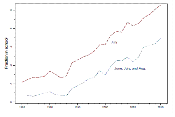
Figure 4b: Potential labor demand and labor supply explanations for declining youth employment: Fraction of 19-21 attending college (school year)
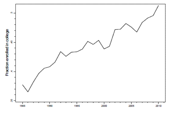
Figure 4c: Potential labor demand and labor supply explanations for declining youth employment: Fraction of the adult (21+) population that is immigrant
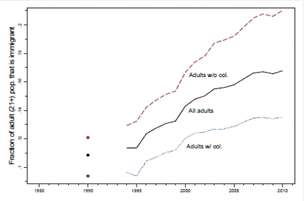
Figure 4d: Potential labor demand and labor supply explanations for declining youth employment: Fraction of employed adults (21+ w/o college) in teen jobs
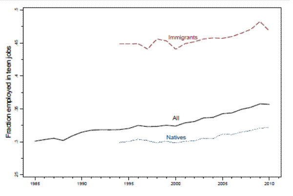
Figure 7a: Relationship between changes in teen employment rates and changes in labor supply and demand measures: Fraction of 16-17 year olds enrolled in the summer
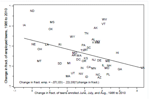
Regression line: change in fract emp = -0.07(0.03) - .22(0.08)*change in fract enrolled.
Figure 7b: Relationship between changes in teen employment rates and changes in labor supply and demand measures: Fraction of 19-21 attending college (school year)
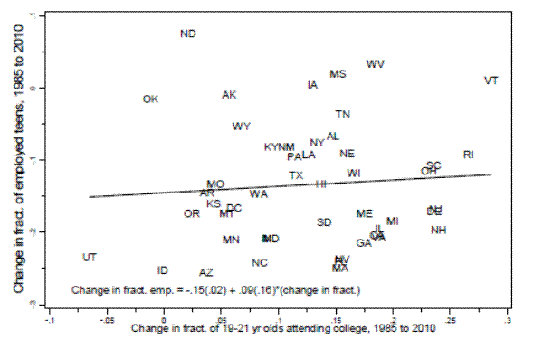
Regression line: change in fract emp = -0.15(0.02) + .09(0.16)*change in fract attending college.
Figure 7c: Relationship between changes in teen employment rates and changes in labor supply and demand measures: Fraction of the adult (21+ w/o col.) population that is immigrant
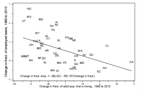
Regression line: change in fract emp = -.09(0.02) + .55(0.16)*change in share immigrant.
Figure 7d: Relationship between changes in teen employment rates and changes in labor supply and demand measures: Fraction of native employed adults (21+ w/o college) in teen jobs
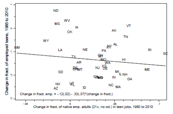
Regression line: change in fract emp = -.12(0.02) - .33(0.37)*change in share of adults in teen jobs.
References
Aaronson, Daniel, Kyung-Hong Park, and Daniel Sullivan. 2006. The decline in teen labor force participation. Economic Perspectives (2006 Q1): 2-18.
Aaronson, Stephanie, Bruce Fallick, Andrew Figura, Jonathan Pingle, and William Wascher. 2006. The recent decline in the labor force participation rate and its implications for potential labor supply. Brookings Papers on Economic Activity 2006:1, 69-134.
Arano, Kathleen and Carl Parker. 2008. How does employment affect academic performance among college students? Journal of Economics 34(2).
Autor, David H. 2010. The polarization of job opportunities in the U.S. labor market: Implications for employment and earnings. Center for American Progress and the Hamilton Project, May 2010.
Autor, David H. and David Dorn. 2009. The growth of low-skill service jobs and the polarization of the U.S. labor market. National Bureau of Economic Research, working paper 15150.
Autor, David H., Frank Levy and Richard J. Murnane. 2003. The skill content of recent technological change: An empirical investigation. Quarterly Journal of Economics 188, no.3 : 1279-1333.
Bartik, Timothy J. 1991. Who benefits from state and local economic development policies. W.E. Upjohn Institute for Employment Research: Kalamazoo, Michigan.
Bishop, John H. and Ferran Mane. 2001. The impacts of minimum competency exam graduation requirements on high school graduation, college attendance and early labor market success. Labour Economics, 8: 203-222.
Camarota, Steven A. and Karen Jensenius. 2010. A drought of summer jobs: Immigration and the long-term decline in employment among U.S.-born teenagers. Backgrounder, May 2010. Center for Immigration Studies. In Adam Gamoran, ed., Will No Child Left Behind Help Close the Poverty Gap? Washington, D.C.: Brookings University Press.
Clements, Matthew T. and Hiroshi Ohashi. 2005. Indirect network effects and the product cycle: Video games in the U.S., 1994-2002. Journal of Industrial Economics, 53(5): 515-542.
Council of Chief State Officers. Various years. Key state education policies on K-12 education: Standards, Graduation, Assessment, Teacher Licensure, Time and Attendance. State Education Assessment Center, Washington DC.
Dee, Thomas S. and Brian A. Jacob. 2007. Do high school exit exams influence educational attainment or labor market performance?
DeSimone, Jeff. 2006. Academic performance and part-time employment among high school seniors. Topics in Economic Analysis and Policy 6(1).
Dustmann, Christian, John Mickleweight, and Arthur van Soest. 2009. In-school labour supply, parental transfers, and wages. Empirical Economics, 37:201-218.
Gong, Tao. 2009. Do parental transfers reduce youths' incentives to work? Labour, 23(4).
Hotz, Joseph V., Lixin Colin Xu, Marta Tienda, and Avner Ahituv. 2002. Review of Economics and Statistics 84(2).
Kahn, Lisa. 2010. The long-term labor market consequences of graduating from college in a bad economy. Labour Economics, 17(1).
Kalenkowski, Charlene Marie and Sabrina Wulff Pabilonia. 2009. Time to work or time to play: The effect of student employment on homework, housework, screen time, and sleep. BLS working paper no. 423.
Kalenkowski, Charlene Marie and Sabrina Wulff Pabilonia. 2010. Parental transfers, student achievements, and the labor supply of college students. Journal of Population Economics 23.
Light, Audrey. 2001. In-school work experience and the returns to schooling. Journal of Labor Economics 19(1).
Lillard, Dean R. and Philip DeCicca. 2001. Higher standards, more dropouts? Evidence within and across time. Economics of Education Review, 20 : 459-473.
Manning, Alan, Maarten Goos, and Anna Salomons. Job polarization in Europe. American Economic Review: Papers and Proceedings 99:58-63.
Morisi, Teresa L. 2008. Youth enrollment and employment during the school year. Monthly Labor Review, February 2008: 51-63.
Morisi, Teresa K. 2010. The early 2000s: a period of declining teen summer employment rates. Monthly Labor Review, May 2010: 23-35.
Mroz, Thomas A. and Timothy H. Savage. 2006. The Long-term effects of youth unemployment. Journal of Human Resources, 41 (Spring):259-293.
National Association of Year-round Education. Statistical Summary of YRE 2007. http://www.nayre.org/STATISTICAL%20SUMMARIES%20OF%20YRE%202007.pdf. Accessed on 8/19/2011.
Neumark, David. 2002. Youth labor markets in the United States: Shopping around vs. staying put. Review of Economics and Statistics 84(3), 462-482.
Newmark, David and William Wascher. 2007. Does a higher minimum wage enhance the effectiveness of the earned income tax credit? National Bureau of Economic Research, Working paper 12915.
Oettinger, Gerald S. 1999. Does high school employment affect high school academic performance? Industrial and Labor Relations Review, 15(1).
Oreopoulos, Philip. 2007. Do dropouts drop out too soon? Wealth, health and happiness from compulsory schooling. Journal of Public Economics 91(11-12): 2213-2229.
Oreopoulos, Philip, Till Von Wachter and Andrew Heisz. 2006. The short- and long-term career effects of graduating in a recession: Hysteresis and heterogeneity in the market for college graduates. National Bureau of Economic Research, working paper no. 12159.
Pabilonia, Sabrina Wulff. 2001. Evidence on youth employment, earnings, and parental transfers in the National Longitudinal Survey of Youth 1997. Journal of Human Resources, 36(4): 795-822.
Ramey, Garey and Valerie A. Ramey. 2009. The rug rat race. National Bureau of Economic Research, working paper no. 15284.
Rothstein, Donna S. 2007. High school employment and youths' academic achievement. Journal of Human Resources.
Ruhm, Christopher. 1997. Is high school employment consumption or investment? Journal of Labor Economics 15(4).
Smith, Christopher L. 2012 (forthcoming). The impact of low-skilled immigration on the youth labor market. Journal of Labor Economics, January 2012.
Stinebrickner, Ralph and Todd R. Stinebrickner. 2003. Work during school and academic performance. Journal of Labor Economics, 21(2).
Sum, Andrew, Paul Garrington and Ishwar Khatiwada. 2006. The impact of new immigrants on young native-born workers, 2000-2005. Technical Report: Center for Immigration Studies.
Tyler, John H. 2003. Using state child labor laws to identify the effect of school-year work on high school achievement. Journal of Labor Economics, 21(2).
von Hippel, Paul T. 2007. What happens to summer learning in year-round schools? Mimeo.
