Skip to: [Printable Version (PDF)] [Bibliography] [Footnotes]

Finance and Economics Discussion Series: 2011-60 Screen Reader version ^♣

Rising Inequality: Transitory or Permanent? New Evidence from a U.S. Panel of Household Income 1987-2006*

Jason DeBacker (Treasury Department)

Bradley Heim (Indiana University)

Vasia Panousi (Federal Reserve Board)

Ivan Vidangos (Federal Reserve Board)

Keywords: Income inequality, variance decomposition, error-components models, transitory vs. permanent

Abstract:

We use a new and large panel dataset of household income to shed light on the permanent versus transitory nature of rising inequality in individual male labor earnings and in total household income, both before and after taxes, in the United States over the period 1987-2006. Due to the quality and the significant size of our dataset, we are able to conduct our analysis using rich and precisely estimated error-components models of income dynamics. Our main specification finds evidence for a quadratic heterogeneous income profiles component and a random walk component in permanent earnings, and for a moving-average component in autoregressive transitory earnings. We find that the increase in inequality over our sample period was entirely permanent for male earnings, and predominantly permanent for household income. We also show that the tax system, though reducing inequality, nonetheless did not materially affect its increasing trend. Furthermore, we compare our model-based findings against those of simpler, non-model based inequality decomposition methods. We show that the results for the trends in the evolution of the permanent and transitory variances are remarkably similar across methods, whereas the results for the shares of those variances in cross-sectional inequality differ widely. Further investigation into the sources of these differences suggests that simpler methods produce erroneous decompositions because they cannot flexibly capture the relative degree of persistence of the transitory component of income.

JEL Classification: C33, D31, J31

1 Introduction

An extensive literature has documented a large increase in income inequality in the United States in recent decades. In this paper, we ask whether this observed increase in cross-sectional inequality reflected an increase in permanent or in transitory inequality. By permanent, we mean an increase in long-run inequality, or growing dispersion in permanent incomes. By transitory, we mean greater short-run variability in incomes, or individuals moving around more within the income distribution at relatively short frequencies of one to a few years.

The distinction between permanent and transitory inequality is important for two main reasons. First, it is useful in evaluating the proposed explanations for the documented increase in annual cross-sectional inequality. For example, if rising inequality reflects solely an increase in permanent inequality, then consistent explanations would include, for example, skill-biased technical change. By contrast, an increase in transitory inequality could be due to increases in income mobility, perhaps driven by growing job instability for all workers. Second, the distinction is useful because it informs the welfare evaluation of cross-sectional inequality increases. Specifically, lifetime income is a measure of long-term available resources, and hence an increase in permanent inequality would be welfare-reducing according to most social welfare functions. By contrast, increasing transitory inequality would have less of an effect on welfare, especially in the absence of liquidity constraints restricting consumption smoothing. Furthermore, as the next section outlines, the literature has not as yet reached a clear consensus about either the nature or the timing of the increases in each inequality component in the last two decades.

One important aspect of our contribution is the use of a new and superior data source to shed new light on the permanent-vs-transitory decomposition of inequality and its evolution over time. In particular, we use a large panel of household income from tax returns to study the permanent-vs-transitory nature of rising inequality in individual (male) labor earnings and in total household income, both before and after taxes, in the United States over the period 1987-2006.¹ Our panel constitutes a one-in-5,000 random sample of the population of U.S. taxpayers. It contains individual-level labor earnings information as well as household-level income information reported in tax forms. It also includes information on the age and gender of the primary and secondary tax filers from matched social security records. Our broadest sample consists of nearly 300,000 observations on 30,000 households, and is therefore substantially larger than the typical survey panels, such as the Panel Study of Income Dynamics (PSID), used to address related questions in the literature. In addition, our data are not subject to top-coding, and are less likely to be affected by measurement error, compared to survey data.

The quality and size of our dataset allow us to start the analysis by precisely estimating rich error-components models of income dynamics. In particular, error-components models fully specify the process that generates income over time, and can be used to decompose the cross-sectional variance of log income-our measure of inequality-into permanent and transitory parts. This way, we can explore in detail the role of permanent and transitory income components for the evolution of inequality. Indeed, one of the main advantages of such models is that they are sufficiently detailed and flexible to be able to capture many facets both of the autocorrelation of earnings and of the evolution of earnings over the lifecycle. We therefore view the fact that we can use the large size of our data to ensure that our models are very precisely estimated as one of the main contributions of our paper.

We next expand our analysis to explore simpler, approximate decomposition methods that have been used in the literature to examine the permanent-vs-transitory nature of inequality. Here, one important aspect of our contribution is that we investigate the relation across the different inequality-decomposition methods, model-based as well as non-model-based, and we propose an explanation for the differences across methods. This is important because, in the existing literature, it is impossible to discern whether the differences across studies are due to the different data or to the different methodologies used. By contrast, we clarify the connections across different methods and we propose one way of thinking about the variety of results they yield. Hence, our analysis could provide guidance for researchers as to the potential outcomes of choosing between different methods.

Turning to the details of our error-components models, our data indicate that male labor earnings are best described by a combination of permanent and transitory components with the following features. First, permanent earnings, whose relative importance varies over calendar time, are captured by the sum of a quadratic heterogeneous income profiles component and a random walk component. Second, transitory earnings are characterized by an ARMA(1,1) process with year-specific innovation variances. Transitory earnings turn out to be relatively persistent (the autoregressive coefficient in our baseline specification is 0.63), despite the inclusion of both heterogeneous income profiles and a random walk in permanent earnings. For household income, the main difference is that the data provide less support for the inclusion of a random walk component in permanent income.

Our main findings on the permanent-vs-transitory decomposition of inequality are as follows. For male labor earnings, we find that the entire increase in cross-sectional inequality over the 1987-2006 period was permanent. In particular, we find that the permanent variance of (log) male earnings increased over this period, while the transitory variance did not. In terms of the permanent-vs-transitory makeup of the cross-sectional variance of male earnings at a single point in time, our preferred model specification implies that, on average, 65% of the total variance of male labor earnings was permanent, while 35% was transitory.

For total household income, we find that the large increase in inequality over our sample period was predominantly, though not entirely, permanent. For this broader income category, both the permanent and the transitory parts of the cross-sectional variance increased, with the permanent variance contributing two thirds and the transitory variance one third of the increase in the total cross-sectional variance. Furthermore, the increase in the transitory component reflected an increase in the transitory variance of spousal labor earnings, transfer income, and investment income.

We extensively explore the sensitivity of our analysis to model specification. We show that the results for the trends in the permanent and transitory variances are remarkably robust across model specifications. However, the shares of cross-sectional inequality attributed to the permanent and transitory income components at a given point in time are quite sensitive to the specification. For instance, the transitory share of total cross-sectional inequality ranges from 27% to 60%, depending on the model used. We examine the reasons for these differences and we show that they reflect differences in the (relative) degree of persistence in the transitory earnings process across the various model specifications. Intuitively, when transitory earnings are less persistent, then more of the persistence in the earnings data will be attributed to the permanent component, leading to a larger role assigned to permanent earnings overall. Conversely, when transitory earnings are allowed to be more persistent, then more of the persistence in the data will be picked up by the transitory part, leading to a larger role played by the transitory earnings component.

Turning to the comparison with simpler methods, we look in particular into two approximate methods that decompose the cross-sectional variance into permanent and transitory parts without explicitly using error-components models. These methods essentially define permanent income as the average of annual income over a certain period of time, and then transitory income as the deviations of annual income from that average. Here, we find that the results for the trends of the permanent and transitory variance components are surprisingly robust across methods, and that therefore the approximate methods corroborate our model-based results for the inequality trends.² However, the permanent and transitory shares of the cross-sectional variance turn out to be very sensitive to the method used. We then propose that the reasons for these differences are closely related to the reasons for the differences across the different model specifications. In particular, the approximate methods we consider do not allow for persistence in transitory income. As a result, they attribute to the permanent income component part of what is in reality a transitory (though serially correlated) shock, thereby overstating the importance of the permanent part of inequality. In other words, the simpler decompositions rely on restrictions that are strongly rejected by the data. Clearly, the share of cross-sectional inequality attributed to the permanent versus the transitory component will have important quantitative and policy implications for the welfare costs of income inequality. Therefore, our analysis provides significant guidance in that direction and it indicates that the search for the appropriate inequality-decomposition method needs to carefully consider the nature of the data, with particular emphasis on the relative degree of persistence in the transitory component of income.

Finally, our tax return data also allow us to examine in detail the role of the federal tax system for the evolution of income inequality. In particular, we investigate whether the evolution of inequality for after-tax household income differs materially from the evolution of inequality for pre-tax income. Our measure of after-tax household income reflects all federal personal income taxes, including all refundable tax credits, as well as payroll taxes. We find that the cross-sectional variance of after-tax income is on average 15% smaller than the variance of pre-tax income, reflecting the overall progressivity of the U.S. federal tax system. On net, however, the effect of the tax system in reducing income inequality appears quite stable over the sample period. In other words, the tax system does not appear to have significantly altered the trend toward rising inequality, despite the large changes in tax policy over this period.

The rest of the paper is organized as follows. The next section discusses the related literature and places our results in the context of existing studies. Section 3 describes our dataset, our sample selection, and the trends in income inequality in our data. Section 4 introduces our error-components models and discusses their estimation. Section 5 presents the model estimates for male labor earnings and uses the estimated models to decompose the cross-sectional variance into permanent and transitory parts. The section then examines the sensitivity of the results to model specification. Section 6 compares our model results to those from alternative methods of analysis and discusses the reasons for the differences across methods. Section 7 examines total household income and the role of the U.S. federal tax system for the evolution of income inequality. Section 8 describes several robustness tests, and section 9 concludes. Technical details and additional results are provided in the Appendix.

2 Related Literature

An extensive literature has documented a large increase in labor earnings inequality in the U.S. in recent decades.³ A small branch of the literature has attempted to determine whether this increase in cross-sectional inequality reflected an increase in permanent or in transitory inequality. The earlier studies, including Gottschalk and Moffitt (1994); Moffitt and Gottschalk (1995); and Haider (2001), all use PSID data, and generally conclude that a substantial part (as much as one half) of the increase in cross-sectional inequality in the 1970s and early 1980s was transitory. There are very few studies analyzing the last two decades, although earnings inequality has continued to increase. Furthermore, the results across studies are not conclusive. For example, using the PSID, Gottschalk and Moffitt (2008) find that the transitory variance has not increased after the mid-to-late 1980s, whereas Heathcote, Perri, and Violante (2010) conclude that the transitory variance rose substantially in the 1990s. Kopczuk, Saez, and Song (2010), using Social Security earnings data, find that the increase in inequality from the 1970s to the early 2000s was entirely permanent. However, they use only a simple approximate decomposition method and their findings contradict the more-established results of the earlier literature for the 1970s and early 1980s, raising doubts about the factors driving their analysis for the more recent period as well. In this paper, we conclude that the increase in inequality since the mid-to-late 1980s has been entirely permanent. Furthermore, we confirm this finding with a variety of model specifications, as well as different decomposition methods, thereby obtaining remarkably robust results.

Inequality in total household income has also increased in recent decades, as documented, among others, by Krueger and Perri (2006); and Heathcote, Perri, and Violante (2010). The only studies that have in some way attempted to decompose the increase in household income inequality into permanent and transitory parts are Gottschalk and Moffitt (2009); Primiceri and van Rens (2009); and Blundell, Pistaferri, and Preston (2008). Gottschalk and Moffitt (2009) use simply an approximate method and provide only suggestive evidence of an increase in the transitory variance starting in the mid-1980s, without conducting a full analysis. By contrast, Primiceri and van Rens (2009), utilizing repeated cross-sections on income and consumption from the Consumer Expenditure Survey (CEX), find that all of the increase in household income inequality in the 1980s and 1990s reflected an increase in the permanent variance. Our results indicate that, for the increase in the cross-sectional variance of household income, the transitory variance did play some role, though not as prominently as Gottschalk and Moffitt (2009) seem to suggest.⁴ Furthermore, we show that the increase in the transitory variance of household income reflected an increase in the transitory variance of spousal labor earnings, transfer income, and investment income.

Our paper is also related to a recent literature that has analyzed the trends in the dispersion of short-term income changes, or income volatility. The findings in this literature have been more consistent across different studies. For instance, a 2008 study by the Congressional Budget Office (CBO); Sabelhaus and Song (2009); Celik, Juhn, McCue, and Thompson (2011); and Shin and Solon (2011), all find that the volatility of male earnings did not increase between the 1980s and the early 2000s.⁵ Our male labor earnings data are consistent with the findings in this literature, as we document no increase in male earnings volatility. However, we do find an increase in the volatility of total household income.

Finally, our paper also contributes to a literature that models and estimates the dynamics of labor income. In particular, there is a long standing debate in this literature concerning the nature of individual labor earnings processes. According to one view, individuals face similar lifecycle earnings profiles and are subject to highly persistent (permanent) earnings shocks, so that permanent earnings are best reflected by a random walk component. See, for example, Hryshko (2010) for a recent study favoring this specification. According to the second view, individuals face heterogeneous lifecycle earnings profiles and are subject to less persistent shocks, so that permanent earnings are best captured by a "heterogeneous income profiles" component. See, for instance, the papers by Baker (1997); and Guvenen (2009).⁶ Our baseline model nests both specifications. For (male) labor earnings, we find that the data support the inclusion of a heterogeneous income profiles component as well as a random walk component. Furthermore, our data support a quadratic specification of heterogeneous income profiles. This is because, in our data, the lifecycle profile of the cross-sectional variance, controlling for either year or cohort effects, is concave in the earlier part of the lifecycle, and convex in the later part. The heterogeneous income profiles component in our baseline model implies that the lifecycle profile of the variance is a cubic polynomial in age, which fits the profile in our tax data well. Overall, we find stronger support for the (quadratic) heterogenous income profiles than for the random walk: The restriction that the variance of the innovation of the random walk component is zero is rejected at a 5% level but not at a 1% level. For total household income, we find less support for a random walk component, whose inclusion depends on the specific sample, on the level of the minimum threshold used to exclude low-income observations, and on whether the income data are before of after taxes.

3 Data

This section describes our panel of income tax returns, our sample selection, and the income inequality trends observed in our data over the period 1987-2006.

3.1 Panel and Variable Description

We use data from a twenty-year panel of tax returns spanning the period 1987-2006. To create this panel, we merged returns from an existing 1987-1996 Statistics of Income (SOI) panel, kept at the Treasury, with returns from cross-sectional files from 1997-2006. We then cut the sample to returns for which the primary filer had a social security number ending in one of two four-digit combinations. The resulting panel (with two exceptions noted below) is a one-in-5,000 random sample of tax units followed over 1987-2006.⁷ Each of the data sources is next described in turn.

The 1987-1996 panel was collected by the SOI and is kept at the Treasury Department. The panel started with a stratified random sample of taxpayers who filed in 1987, a subset of which was chosen based on the primary filer's social security number ending in one of two four-digit combinations.⁸ $^{,}$ ⁹ All individuals represented on the tax return of a member of this cross section, including secondary taxpayers on joint returns and dependents, were considered to be members of the panel. Over the following nine years, the SOI division included in the panel all returns that reported any panel member as a primary or secondary taxpayer, including tax returns filed by panel members who were dependents of another taxpayer. To keep the sample representative of the tax filing population in subsequent years, tax returns from tax years 1988 through 1996 were added to the panel if the primary filer had an social security number ending in one of the two aforementioned four-digit combinations but did not file a return in 1987.¹⁰ In addition to information from each tax form, the dataset includes information on age and gender of the primary and secondary filers obtained from matched social security records.

The 1997-2006 data come from yearly cross-sections collected by the SOI, and also maintained at the Treasury. Like the 1987 sample described above, a stratified random sample was collected in each of these years, consisting partly of a strictly random sample based on the last four digits of the primary filer's social security number. Each cross-section contains information from tax forms, and merged information on age and gender of the primary and secondary filers from social security records.

As noted above, in our estimation sample we only include returns from either of these two data sources where the primary taxpayer's social security number had one of the two 1987 original four-digit endings, resulting in a one-in-5,000 random sample. The panel is not balanced, as some taxpayers drop out of the sample due to death, emigration, or falling below the tax filing thresholds, while others enter because of immigration or becoming filers.

The ideal measure of individual-level earnings for this study is gross labor income before any amounts are deducted for health insurance premiums or retirement account contributions. However, our data do not contain such a variable, and hence we use a measure of labor income that is as close to gross labor income as is possible, using tax data. For this, we take taxable wages, and we add reported contributions to retirement savings accounts. This measure of labor income will include all income that a taxpayer's employer has reported, namely wages, salaries, and tips, as well as the portion of these that is placed in a retirement account. Since our data do not include information on the health insurance premiums paid by the taxpayer and excluded from taxable wages, our measure of labor income will exclude those amounts. Our measure also excludes any income earned from self-employment.

For pre-tax total household income, we start with the "total income" amount of income reported. This variable includes wages and salaries, dividends, alimony, business income, income from rental real estate, royalties, and trusts, unemployment compensation, capital gains, and taxable amounts of interest, IRA distributions, pensions, and social security benefits. To this, we add back nontaxable interest, IRA distributions, pensions, and social security benefits.

There is some debate as to whether capital gains should be included in the measure of household income, as the amount of capital gains realized in a particular year and reported on the tax form may include gains that accrued in the past. Hence, it may make household income appear "lumpier" than it actually is, since income will be higher in years when gains from prior years are realized, and lower in years when gains accrued but were not realized. However, excluding capital gains will result in the measure of household income being too low for any taxpayer who had gains in that year (whether or not they were realized), and this downward bias will be quite large for taxpayers whose primary source of income is from investments. On balance, we feel that this concern is more important, and therefore we include capital gains in our benchmark measure of household income.¹¹

For after-tax household income, we start with the measure of pre-tax household income described above. We then subtract the amount of "total taxes" which captures total income taxes (including self-employment taxes) after non-refundable tax credits are taken into account. Next, we subtract the total amount of FICA taxes owed on the earned income of the couple. This is done to ensure that all federal taxes (including income and payroll taxes) are included for all taxpayers, regardless of whether they are wage and salary workers or self-employed. Finally, we add refundable tax credits (including the earned income tax credit and the refundable portion of the child tax credit) to arrive at our measure of after-tax household income.

3.2 Sampling Change and Demographics

There was a change in the sampling frame of our data in 1996. As a result of this change, we are missing two groups of filers in the pre-1996 period: Dependent filers in 1987 over the period 1987-1996, and non-dependent primary filers in 1988-1996 who were either dependent or secondary filers in 1987. These two groups primarily consist of young (in the case of dependents) or female (in the case of secondary) taxpayers. The effect of missing these returns is therefore likely to be very small when we examine the labor income of males in their earning years, though it may be larger when we examine household income.

To address potential issues introduced by this sampling change, we carry out our analysis of household income using two alternative samples. First, we analyze household income using the same sample of households that we use to analyze male earnings, namely male-headed households, as this sample was essentially unaffected by the sampling change. Second, we analyze household income using a sample with either a male or a female primary filer (see section 3.3). We are interested in this broader sample because it represents the entire population of tax units in the U.S., and not just those with a male primary filer.

One additional point to be mentioned is that our tax data contains fewer socio-demographic variables, compared to surveys like the PSID. Most importantly, though we have information on age and gender of the primary and secondary filer, we do not have information on education and race. We also lack information on hours of work, and hence our analysis will focus on annual earnings, as opposed to wage rates.

3.3 Sample Selection

For the case of individual earnings, we restrict our sample to male primary filers, as is standard in the literature, because female movements in and out of the labor force introduce discontinuities in the earnings process. For household income, we carry out our analysis using two alternative samples. The first sample includes households with a male primary filer only. This avoids confounding the effects of using a broader measure of income (total household income) with the effects of using a broader sample of households. In addition, this sample was not affected by the change in sampling frame discussed in section 3.2. The second sample includes households with either a male or a female primary filer, and is representative of the population of U.S. taxpayers.

For both male earnings and household income, we restrict our sample to households with a primary filer aged between 25 and 60. We impose this restriction because individuals in this age group are likely to have completed most of their formal schooling and are sufficiently young not to be too strongly affected by early retirement.

For both male earnings and household income, we exclude earnings/income observations below a minimum threshold. For male earnings, since tax records do not provide information on employment status or hours of work, we can exclude individuals with presumably weak labor force attachment only by dropping low-earnings observations. Turning to household income, we note that households with sufficiently low income are not required to file taxes, although many actually do, so as to claim refundable tax credits, such as the earned income tax credit. In order to treat low-income observations consistently, we exclude observations with reported household income below a minimum threshold.¹² We take the relevant threshold to be one fourth of a full year full time minimum wage in 2004 ($2,575 in 2004), and indexed for other years by nominal average wage growth.¹³

After imposing the restrictions above, we end up with a male earnings sample of 189,424 person-year observations. We refer to this sample as our `male earnings' sample. We use this sample to analyze not only male earnings, but also household income, both before and after taxes. Our broader sample for household income, which includes households with either a male or a female primary filer, contains 294,910 observations. We refer to this sample as our `full' household sample. Table I shows the number of observations, the mean, and the standard deviation for male earnings, pre-tax household income, and after-tax household income for each one of our samples.

3.4 Income Inequality Trends 1987-2006

We begin by documenting the evolution of inequality over time for male earnings and for household income, before and after taxes, in our panel of tax returns. Figures I (a) and I (b) show the cross-sectional variance (of the log) and the Gini coefficient, respectively, for male earnings, pre-tax household income, and after-tax household income. The figures show an increase in the variance and in the Gini coefficient for all three measures of income over 1987-2006. For example, the cross-sectional variance (of the log) increases by 0.11 points or 18% for male earnings, by 33% for pre-tax household income, and by 28% for after-tax household income.¹⁴ In general, inequality in individual earnings is lower than inequality in household income. Furthermore, inequality in after-tax household income is lower than inequality in pre-tax household income, reflecting the progressivity of the U.S. tax system.

These inequality trends in our data are consistent with trends that have been documented in many other U.S. studies. In the remainder of the paper, we focus on the cross-sectional variance (of the log) of earnings and household income as our measure of inequality, and we investigate whether the increase in the variance shown here represented an increase in permanent inequality versus an increase in transitory inequality.

4 Error-Components Models

Our baseline model is as follows. Let $y_{a,t}^{i}$ denote log income, where indexes individual, age, and calendar year.¹⁵ Log income is given by:

$\displaystyle y_{a,t}^{i}=g(\zeta _{t};X_{a,t}^{i})+\xi _{a,t}^{i}$ ,

(1)

where $X_{a,t}^{i}$ is a vector of observable characteristics,

is the part of log income that is common to all individuals conditional on $X_{a,t}^{i}$ , $\zeta _{t}$ is a vector of parameters (possibly including parameters that depend on calendar year

), and $\xi _{a,t}^{i}$ is the unobservable error term. As is common in the literature on income dynamics, we will remove the income variation that is due to observables, $X_{a,t}^{i}$ , and focus on the dynamics of the error term, $\xi _{a,t}^{i}$ .

We model $\xi _{a,t}^{i}$ as consisting of a permanent and a transitory component:

$\displaystyle \xi _{a,t}^{i}=\underbrace{\lambda _{t}\text{ \textperiodcentered\ }(\alpha ^{i}+\beta ^{i}a+\gamma ^{i}a^{2}+r_{a,t}^{i})}+\underbrace{z_{a,t}^{i}} ,\quad \quad \text{where}$

(2)

permanent transitory

$\displaystyle r_{a,t}^{i}=r_{a-1,t-1}^{i}+\epsilon _{a,t}^{i}$

(3)

$\displaystyle z_{a,t}^{i}=\rho z_{a-1,t-1}^{i}+\pi _{t}$ $\textperiodcentered$ $\displaystyle \eta _{a,t}^{i}+\theta$ $\textperiodcentered$ $\displaystyle \pi _{t-1}$ $\textperiodcentered$ $\displaystyle \eta _{a-1,t-1}^{i}$

(4)

$\displaystyle \alpha ^{i}$	$\displaystyle \sim$	$\displaystyle iid(0,\sigma _{\alpha }^{2}), \beta ^{i}\sim iid(0,\sigma _{\beta }^{2}), \gamma ^{i}\sim iid(0,\sigma _{\gamma }^{2}),$	(5)
$\displaystyle cov(\alpha ^{i},\beta ^{i})$	$\displaystyle =$	$\displaystyle \sigma _{\alpha \beta }, cov(\alpha ^{i},\gamma ^{i})=\sigma _{\alpha \gamma }, cov(\beta ^{i},\gamma ^{i})=\sigma _{\beta \gamma }, \notag$	(6)
$\displaystyle \epsilon _{a,t}^{i}$	$\displaystyle \sim$	$\displaystyle iid(0,\sigma _{r}^{2}), \eta _{a,t}^{i}\sim iid(0,\sigma _{z}^{2}) \notag$	(7)

The permanent income part consists of an individual-specific, time-invariant component, $\alpha ^{i}$ , a quadratic heterogeneous income profiles component, $\beta ^{i}a+\gamma ^{i}a^{2}$ , and a random-walk component, $r_{a,t}^{i}$ . These components are pre-multiplied by the year-specific factor loading, $\lambda _{t}$ , which allows the relative importance of permanent income to vary over calendar time. The components $\alpha ^{i}$ , $\beta ^{i}$ , and $\gamma ^{i}$ are allowed to be freely correlated, with $cov(\alpha ^{i},\beta ^{i})=\sigma _{\alpha \beta }$ , $cov(\alpha ^{i},\gamma ^{i})=\sigma _{\alpha \gamma }$ , and $cov(\beta ^{i},\gamma ^{i})=\sigma _{\beta \gamma }$ .

When only allowing for a linear heterogeneous income component, we find that the data strongly reject that specification. Allowing for a quadratic heterogeneous income profiles component improves the fit of the model, and the quadratic specification cannot be rejected, even if a random walk component is also included. In particular, the quadratic heterogeneous income profiles component improves the fit of the evolution of the cross-sectional variance of earnings/income over the lifecycle. This is because, in our data, the lifecycle profile of the cross-sectional variance, controlling for either year or cohort effects, is concave in the earlier part of the lifecycle, and convex in the later part. The heterogeneous income profiles component in our model implies that the lifecycle profile of the variance is a cubic polynomial in age, which fits the profile in our tax data well.¹⁶

The transitory component in the model, $z_{a,t}^{i}$ , is specified as an process. The transitory innovations, $\eta _{a,t}^{i}$ , are multiplied by the year-specific factor loadings, $\pi _{t}$ , which allow the variance of the innovations, and hence the relative importance of the transitory component, to vary by calendar year.

Notice that, in the model above, permanent income shocks, $\epsilon _{a,t}^{i}$ , are defined as shocks that shift the path of income permanently, whereas transitory shocks, $\eta _{a,t}^{i}$ , are defined as shocks with effects that eventually disappear. Nonetheless, since transitory shocks are allowed to be serially correlated, it could take several years for their effects to die out. In other words, the permanent component is defined as capturing shocks that are not mean-reverting, whereas the transitory component is defined as capturing mean-reverting shocks.

For purposes of robustness, we are also interested in exploring how our decomposition of the cross-sectional variance into permanent and transitory parts depends on model specification. Therefore, we also examine three alternative models, which we call restricted models RM1, RM2, and RM3. These models are obtained by imposing the following restrictions on our baseline model:

(i) RM1: $\sigma _{\beta }^{2}=\sigma _{\gamma }^{2}=\sigma _{\alpha \beta }=\sigma _{\alpha \gamma }=\sigma _{\beta \gamma }=0$ (no heterogeneous income profiles)

(ii) RM2: $\sigma _{r}^{2}=0$ (no random walk)

(iii) RM3: $\theta =0$ (no MA transitory errors) In what follows we will demonstrate that the data strongly reject the restrictions imposed by all three models RM1, RM2, and RM3, thereby establishing our preference for our baseline model.

4.1 Estimation

Estimation of our error-components models proceeds in two stages. In the first stage, we construct residuals from regressions of log earnings (or log income) against observables, $\hat{\xi}_{a,t}^{i}=y_{a,t}^{i}-g(\hat{\zeta} _{t};X_{a,t}^{i})$ . In particular, for male earnings, we estimate least-squares regressions, separately for each year, of log earnings against a full set of age dummies, thus removing the predictable lifecycle earnings variation. For household income, we regress, separately for each year, log household income on a full set of age dummies for the primary tax filer, indicators of gender and marital status for the primary filer, and a full set of dummies for the number of children (up to ten) in the household.¹⁷ Since the tax data do not contain information on race and education, the corresponding part of income variation will remain in the residuals and will add to the variation attributed to the permanent component. The Appendix describes our first-stage regressions in more detail.

In the second stage, we estimate all model parameters (other than $\zeta _{t}$ ) using a minimum distance estimator that matches the model's theoretical variances and autocovariances to their empirical counterparts. The error-components model in equations (2)-(5) implies a specific parametric form for each variance and autocovariance of residual income, given normalized age , calendar year , and lead . These theoretical variances and autocovariances, denoted by , are functions of the model parameters $\sigma _{\alpha }^{2},\sigma _{\beta }^{2},\sigma _{\gamma }^{2},\sigma _{\alpha \beta },\sigma _{\alpha \gamma },\sigma _{\beta \gamma },\sigma _{r}^{2},\rho ,\theta ,\sigma _{z}^{2}$ , and $\lambda _{t},\pi _{t}$ for . We estimate these model parameters by minimizing the distance between the theoretical variances and autocovariances implied by the model, and their empirical counterparts, which we compute from our longitudinal tax return data for , , and . This yields over 6,000 variances and autocovariances that are matched in estimation. Our minimum distance estimator uses a diagonal matrix as the weighting matrix, with weights equal to the inverse of the number of observations used to compute each empirical statistical moment. We do not use an optimal weighting matrix for reasons discussed in Altonji and Segal (1996). The basic intuition for identification of the permanent and transitory components is that the contribution of the transitory component to the autocovariance of income between two periods vanishes as the distance between the periods gets large enough.

4.2 Variance Decomposition

After estimating our baseline model in equations (2)-(5), we can use it to determine its implications for annual cross-sectional income inequality for each income measure, whether at the individual or at the household level. In other words, we will use the estimated model to decompose the cross-sectional variance of log (residual) income. In particular, for each calendar year between 1987 and 2006, the model implies a specific value for the total cross-sectional variance, the permanent variance, and the transitory variance of log (residual) income, as a function of the model parameters and given an age distribution. We compute these variances implied by the estimated model, assuming an age distribution equal to the actual empirical age distribution in our sample.¹⁸ Note that the evolution of the permanent variance and the transitory variance is primarily determined by the estimates of the $\lambda _{t}$ and $\pi _{t}$ parameters, respectively. We also repeat this procedure to derive inequality decompositions into permanent and transitory components for each one of the restricted models RM1, RM2, and RM3.

5 Male Earnings

In this section we present model estimates for male earnings, and we use our estimated models to decompose the cross-sectional variance of (residual) log male earnings into permanent and transitory components. We also extensively explore the sensitivity of our results to alternative model specifications, and we provide a detailed discussion for the outcomes of the comparison across different models.

5.1 Baseline Model Estimates and Inequality Decomposition

Table II presents estimates for our error-components models, baseline and restricted, for (residual) male earnings. Columns 1a and 1b display point estimates and standard errors for our baseline model. We note that all model parameters are precisely estimated. Starting with the permanent earnings component, the parameter estimates (other than the $\lambda _{t}$ parameters) are $\hat{\sigma}_{\alpha }^{2}=.2487$ , $\hat{\sigma}_{\beta }^{2}=.0019$ , $\hat{\sigma}_{\gamma }^{2}=.0000018$ , $\hat{\sigma}_{\alpha \beta }=-.0092$ , $\hat{\sigma}_{\alpha \gamma }=.00024$ , $\hat{\sigma} _{\beta \gamma }=-.00006$ , and $\hat{\sigma}_{r}^{2}=.0122$ . All of these parameter estimates are statistically significant, so the data appear to support the inclusion of both (quadratic) heterogeneous income profiles and a random walk in permanent earnings. For the transitory earnings component, the parameter estimates (other than the $\pi _{t}$ parameters) are $\hat{\rho }=.6281$ , $\hat{\theta}=-.3302$ , and $\hat{\sigma}_{z}^{2}=.1986$ . The estimate of $\rho$ implies a relatively persistent transitory earnings process, despite the presence of both heterogeneous income profiles and a random walk in permanent earnings. In addition, the data appear to support the presence of moving average innovations in the autoregressive transitory earnings (the estimate $\hat{\theta}=-.3302$ has a standard error of .0153 ). We will return to these points in the section 5.2.

The inequality decomposition implied by our baseline model is presented in Figure II, panel (a). Here, the top line, which shows the total cross-sectional variance implied by the estimated model, is very close to the empirical cross-sectional variance of log (residual) male earnings in our sample. Hence, our baseline specification is sufficiently flexible to fit the evolution of the cross-sectional variance over calendar time. It can also be seen that the baseline model attributes, on average, 65% of the total variance to the permanent component of earnings, and the remaining 35% to the transitory component. More importantly for our purposes, the permanent variance increases by 30% between 1987 and 2006, while the transitory variance fluctuates over the twenty-year period, but does not increase, on net. In fact, the transitory variance is 2% lower in 2006, compared to 1987. In other words, the entire 17% increase in the total cross-sectional variance of (residual log) male earnings is driven by an increase in the permanent earnings variance, thus reflecting an increase in permanent inequality.

5.2 Robustness: Alternative Model Specifications

In Table II, Columns 2a through 4b show parameter estimates and standard errors for the restricted models RM1 (no heterogeneous profiles), RM2 (no random walk), and RM3 (no MA component). For each of the restricted models, all model parameters are precisely estimated. In Figure II, the corresponding inequality decompositions are presented in panels (b)-(d). As was the case for the baseline model, here too the total cross-sectional variance implied by each restricted model is very close to the empirical cross-sectional variance in our sample. This means that the restricted models are also flexible enough to fit the evolution of the cross-sectional variance over calendar time. Furthermore, the trends in the permanent and transitory variances are remarkably robust across model specifications. In particular, all models find that the permanent variance increases over the sample period, while the transitory variance does not, and also that the temporal pattern of the evolution of both variances is remarkably similar. Thus, all specifications imply that the entire increase in the total cross-sectional variance of log residual male earnings over the period 1987-2006 was driven by an increase in the permanent part of the variance, reflecting an increase in permanent inequality.

However, the shares of the total cross-sectional variance attributed to the permanent and transitory components differ widely across the different models. Specifically, the transitory share of the total variance, which was 35% for the baseline model, is, on average, 60% for RM1 (no heterogeneous profiles), 43% for RM2 (no random walk), and 27% for RM3 (no MA component). Given this range of results for the decomposition of inequality, we next proceed to examine the source of the differences across model specifications. We will argue that these differences reflect differences in the (relative) degree of persistence in transitory earnings across the various model specifications. Intuitively, when transitory earnings are less persistent, then more of the persistence in the earnings data will be attributed to the permanent component, leading to a larger role assigned to permanent earnings overall. Conversely, when transitory earnings are more persistent, then more of the persistence in the data will be picked up by the transitory part, leading to a larger role played by the transitory earnings component.

We begin by showing the differences in the persistence of transitory earnings implied by the various estimated model specifications. Table III shows, for each model, the fraction of a transitory shock that survives periods after the shock. As column (1) shows, our baseline parameter estimates, $\hat{\rho }=.6281$ and $\hat{\theta}=-.3302$ , imply that 30%, 19%, and 5% of a transitory shock remains after 1, 2, and 5 years, respectively. That is, our baseline model implies a moderate degree of persistence in transitory earnings, despite the inclusion of both heterogeneous income profiles and a random walk component in permanent earnings.

Restricted model RM1 (no heterogeneous profiles), by contrast, yields the estimates $\hat{\rho}=.9238$ and $\hat{\theta}=-.5912$ . The estimate of $\rho$ , in particular, would appear surprisingly high for a transitory earnings component. Indeed, column (2) of Table III shows that these estimates imply that 33%, 31%, and 24% of a transitory shock remains 1, 2, and 5 years after the shock. Moreover, 16% of a transitory shock remains even 10 years after the shock. The reason for this high degree of persistence in transitory earnings is that permanent earnings in model RM1 lack a heterogeneous income profiles component, which would capture part of the persistence in the earnings data. Therefore, a larger share (relative to the baseline) of the persistence in the data is attributed here to the transitory component instead.

At the opposite end, restricted model RM3 (no MA component) yields a very small estimate of the autoregressive parameter, $\hat{\rho}=.2134$ , which implies very little persistence in transitory earnings. In fact, as shown by column (4) of Table III, only 5% percent of a transitory shock remains after 2 years, with essentially no effect remaining 3 years after the shock. Note that, according to our baseline model, the effect of transitory shocks falls rapidly after one period (via $\hat{\theta}=-.3302$ ), but decays more slowly after that (via $\hat{\rho }=.6281$ ). By contrast, under model RM3's restriction that $\theta =0$ , the rapid fall of the effects of a transitory shock after one period can only be captured by the autoregressive parameter $\rho$ , which in turn implies that the estimate of $\rho$ will be pushed downward.

The above discussion illustrates a more general point that is often overlooked in discussions of permanent-transitory decompositions of income. In reality, incomes are subject to many different types of shocks. While some of these shocks might be truly permanent, and some truly transitory, many shocks are likely to have varying degrees of persistence, in between the two extremes. Decomposing income into permanent and transitory components requires taking a stand on what degree of persistence will be considered "permanent" and what degree will be considered "transitory". This choice necessarily involves some arbitrariness. Our approach here is to rely on a carefully specified error-components model that captures as well as possible the entire covariance structure of earnings, building on what has been learned about the dynamic properties of income from the literature on income dynamics. We thus advocate working with the model that best describes the data, which in our case is our baseline model.

In order to further substantiate the claim that our baseline model best fits our data, we next show that the restrictions implied by models RM1, RM2, and RM3 are actually strongly rejected by the data. This implies that the restricted models miss important dimensions of the earnings data, despite capturing the evolution of total inequality and yielding results for inequality trends similar to the baseline model. In other words, it has to be the case that the different results across specifications for the shares of the total cross-sectional variance attributed to the permanent and transitory components are due to aspects of the restricted models that are not supported by the data. Starting with model RM1 (no heterogeneous profiles), a joint test of the restrictions imposed by the model, namely $\sigma _{\beta }^{2}=\sigma _{\gamma }^{2}=\sigma _{\alpha \beta }=\sigma _{\alpha \gamma }=\sigma _{\beta \gamma }=0$ , yields the F statistic , which overwhelmingly rejects those restrictions (the critical F value at a 1% level is 3.02). Similarly, a test of the restriction $\sigma _{r}^{2}=0$ imposed by model RM2 (no random walk) yields a statistic of , which rejects this restriction at a 5% level (though not at a 1% level). Finally, a test of the restriction $\theta =0$ imposed by RM3 (no MA component) yields the statistic , rejecting the null at a 1% level.

Overall, our results support the inclusion of a (quadratic) heterogeneous income profiles component, of a random walk component, and of moving-average innovations in the (autoregressive) transitory component in models of individual male labor earnings. The presence of quadratic heterogeneous income profiles is especially strongly supported in our data. As we show in Figure A.1 of the Appendix, model RM1's restriction of no heterogeneous income profiles leads to a poorer fit in the evolution of the cross-sectional variance of earnings over the lifecycle. In addition, this restriction leads to the largest difference, relative to the baseline model, in the permanent and transitory shares of the cross-sectional variance in Figures II (a)-II (d). Although the data also support the inclusion of a random walk component in the error-components model, that support is somewhat weaker, as evidenced by the finding above that model RM2's restriction of no random walk is rejected at a 5% level, but not at a 1% level. Furthermore, section 7 shows that, when working with total household income, we cannot reject model RM2's restriction of no random walk.

6 Comparison to Alternative Decomposition Methods

In this section, we expand our analysis to explore simpler, approximate decomposition methods that do not rely on models and that have been used in the literature to examine the permanent-vs-transitory nature of inequality. We also investigate the relation across the different inequality-decomposition methods, model-based as well as non-model-based, and we propose an explanation for the differences across methods. By clarifying the connections across methods, we hope to propose one way of thinking about the variety of results they yield as well as some guidance for the potential outcomes of different methodological choices.

6.1 KSS and BPEA methods

Here, we consider two approximate inequality-decomposition methods which basically define permanent income as the average of annual income over a certain period of time, and then transitory income as the deviations of annual income from that average. The first is a simple and intuitive method that does not explicitly rely on any model. This method, used in Kopczuk, Saez, and Song (2010) and referred to as `KSS' here for convenience, defines person 's permanent earnings in year as the average of person 's annual log earnings (or residual log earnings) over a -year period centered around . Transitory earnings for person in year are then defined as the difference between person 's current annual earnings at and permanent earnings in the same year. The permanent and transitory variances are next calculated as the variances, across individuals, of permanent and transitory earnings, respectively.

Figure III (a) shows the decomposition of the cross-sectional variance of (residual) male earnings into permanent and transitory parts using the KSS method with parameter .¹⁹ Two points are worth noting here. First, in terms of the trends, the increase in the cross-sectional variance is again entirely driven by the permanent component, as it was in our model-based results. Second, in terms of the relative shares, this method attributes on average 87% of the cross-sectional variance to the permanent component, and only 13% to the transitory component, as opposed to 65% and 35%, respectively, in our baseline model. In other words, the KSS method attributes an overwhelmingly large part of the variance to the permanent earnings component.

In order to see why this is the case, note that the KSS decomposition depends crucially on the value of -the number of years used to define permanent earnings. We show in Figure A.2 of the Appendix that, as increases, the permanent share falls and the transitory share rises. For example, for and 9 years, the transitory share is 8%, 13%, 16%, and 18%, respectively. The choice of is obviously arbitrary. Nonetheless, using large values of is impractical, as the construction of the decomposition leads to the loss of data at the endpoints of the sample (for example, using would lead to the loss of 5 years of data at each endpoint of our 20-year sample).²⁰ Furthermore, in the KSS decomposition, "transitory earnings" capture only purely transitory earnings (with no persistence). However, as we have shown, the data provide evidence of moderate persistence in transitory earnings.

We also consider a second approximate variance decomposition method, which was introduced by Gottschalk and Moffitt (1994). Following Moffitt and Gottschalk (2008), we refer to this method as `BPEA'. The BPEA method is similar, though not identical, to the KSS, and we consider it separately because it relies on a simple model of income, which provides a more direct way of relating it to our error-components models.²¹ Specifically, BPEA is based on the simple specification of (residual) log earnings $\xi _{it}=\alpha _{i}+\varepsilon _{it}$ , where $\alpha _{i}$ is purely permanent (time-invariant) and $\varepsilon _{it}$ is purely transitory (). For a -year window centered around each year , BPEA uses the standard formulas from this simple "random effects model" to compute the permanent variance of $\xi _{it}$ as the variance of $\alpha _{i}$ , and the transitory variance of $\xi _{it}$ as the variance of $\varepsilon _{it}$ . To obtain a series of permanent and transitory variance estimates over time, this procedure is repeated for consecutive, overlapping -year moving windows.

Figure III (b) presents the BPEA inequality decomposition. Once again, the decomposition implies that the entire increase in the cross-sectional variance is driven by an increase in the permanent variance. This method (with ) attributes about 80% of the total cross-sectional variance to the permanent component, slightly less than the KSS decomposition, but still quite a bit more than our baseline error-components model. Again, the reason for this difference lies in the simple structure of the model underlying the BPEA decomposition. In particular, note that our baseline model of equations (2)-(5) essentially nests the simpler model upon which BPEA is based, with restrictions $\sigma _{\beta }^{2}=\sigma _{\gamma }^{2}=\sigma _{\alpha \beta }=\sigma _{\alpha \gamma }=\sigma _{\beta \gamma }=\sigma _{r}^{2}=0$ in the permanent component, and $\rho =\theta =0$ in the transitory component (and with our baseline model using the more flexible $\lambda _{t}$ and $\pi _{t}$ for , rather than the -year moving windows). As our results in section 5.2 indicated, these restrictions are strongly rejected in the data.²²

The discussion above suggests that the reasons for the inequality-decomposition differences between our baseline model and the non-model-based methods considered here are in fact closely related to the reasons for the differences across different model specifications. Specifically, the KSS and BPEA approximate methods do not allow for persistence in transitory income. As a result, they attribute to the permanent income component part of what is in reality a transitory (though serially correlated) shock, thereby overstating the importance of the permanent part of inequality. In other words, the simpler decompositions rely on restrictions that are strongly rejected by the data. Therefore, our analysis here indicates that the search for the appropriate inequality-decomposition method needs to carefully consider the nature of the data, with particular emphasis on the relative degree of persistence in the transitory component of income.

6.2 Volatility

Next, we examine the evolution of the standard deviation of changes in male earnings over short horizons. Following Shin and Solon (2011), we refer to this measure as earnings volatility. This measure of dispersion in the cross-sectional distribution of short-run income changes is related, though not equivalent to, the concept of the transitory variance.²³ Figure IV shows the evolution of the standard deviation of one-year (the lower line) and two-year (the upper line) percent changes in (residual) male earnings.

As the figure shows, we find no clear increasing or decreasing trend in male earnings volatility over our sample period. This is consistent with the stable transitory variance of male earnings found in the rest of our decompositions. This finding thus reinforces the result that the increase in male earnings inequality over 1987-2006 was of a permanent nature, as the transitory variance and the volatility of male earnings appear to be overall flat during this period.

7 Household Income

In this section we examine the evolution of the permanent and transitory variance of total household income. As already mentioned in section 3, we carry out the analysis using two alternative samples. First, our `male earnings' sample, which is identical to the sample used in our analysis of male earnings. This sample consists of households with a male primary filer aged 25-60, whose annual labor earnings are above the minimum threshold. Second, our `full' household sample, which mostly adds households with a female primary filer (typically single females).²⁴ As Table I shows, the full sample has 105,544 observations more than the male earnings sample.

The analysis here is performed on residuals from a first-stage regression of log household income on gender, age and filing status of the primary filer, and on a full set of dummies for the number of children (see the Appendix for details). In section 8 we investigate the robustness of our results to alternative treatments of household size and composition.

7.1 Pre-Tax Household Income

Table IV presents point estimates and standard errors for our error-components models estimated on total pre-tax household income data, for both our `male earnings' sample and our broader `full' household sample. Columns 1a-1b show estimates of our baseline model on the male earnings sample. Note that the estimate of the random walk innovation variance $\hat{\sigma} _{r}^{2}=.0014$ (.0059) is not statistically significant. That is, when using our male earnings sample, we cannot reject the hypothesis that $\sigma _{r}^{2}$ is in fact zero. For this reason, we will also present results for restricted model RM2, which imposes $\sigma _{r}^{2}=0$ .²⁵ We have also estimated restricted models RM1 and RM3, but do not show the results here because of space constraints. Columns 2a-2b of Table IV present point estimates and standard errors for model RM2 estimated on our male earnings sample. Note that for this specification, all parameter estimates are statistically different from zero.

Figures V (a) and V (b) present the variance decompositions for our baseline model and for model RM2, both estimated on our male earnings sample.²⁶ Of course, since we cannot reject the hypothesis that $\sigma _{r}^{2}=0$ , the decompositions for the two models are almost identical. In particular, the transitory variance accounts for about 40% of the total variance, which is similar to our finding for male earnings. Moving to the time trends, the transitory variance increased by about 30% over the sample period, mainly in the early 2000s. The permanent variance rose overall by about 45%, showing first a relatively steady increase until around 2000, followed by a moderate decline in the early 2000s and then a resumed increase in the last three years of the sample. All told, the transitory variance contributed about one third of the increase in the total cross-sectional variance. Thus, as in the case of male labor earnings, most of the increase in household income inequality (two thirds) represented an increase in permanent inequality. However, in contrast to male earnings, the transitory variance here did play a role in the increase in household income inequality.

Figure VI shows the evolution of the standard deviation of one-year (the bottom line) and two-year (the top line) percentage changes in total household income on our male earnings sample. As shown by the figure, household income volatility rose 13% for one-year income changes and 12% for two-year income changes, over the sample period. This provides further evidence that the transitory variance did in fact contribute to the increase in the cross-sectional inequality in the case of household income. Furthermore, we have also computed (but do not show) variance decompositions for restricted models RM1 (no heterogeneous profiles) and RM3 (no MA component), as well as for the KSS and BPEA methods, all of which confirm this result.

In going from individual male earnings to total household income, a number of income components are added. We group these components into four main categories: spousal labor earnings, transfer income, investment income, and business income. Transfers are defined here as the sum of alimony received, pensions and annuities, unemployment compensation, social security benefits, and tax refunds. Investment income includes interest, dividends and capital gains. Business income includes income from self-employment, from partnerships, and from S-corporations.²⁷

Next, we examine which component or category of household income is responsible for the increase in the transitory variance of total household income. We start with male labor earnings, and then sequentially (and cumulatively) add each of the other categories of income, namely spousal labor earnings, transfer income, investment income, and business income. For each of the resulting income aggregates, we estimate our error-components models, and we decompose the cross-sectional variance into permanent and transitory parts.²⁸ The decompositions, based on restricted model RM2 (no random walk) and our male earnings sample, are presented in Figure A.3 of the Appendix. The other restricted models lead to similar conclusions. Starting with male earnings, and moving along the series of increasingly broad income aggregates, the changes in the transitory variance between 1987 and 2006 are -2%, 8%, 17%, 29%, and 28%, respectively. This takes us from the slight decrease in the transitory variance of male earnings, to the 28% increase in the transitory variance of total household income that we found earlier. We conclude that each of spousal labor earnings, transfer income, and investment income contributed to the increase in the transitory variance of total household income. Moreover, none of these categories appears to have played a particularly dominant role in driving the increase in the transitory variance of total household income.²⁹

Columns 3a-4b of Table IV present point estimates and standard errors for the baseline and restricted model RM2 using our broader `full' household income sample. The corresponding variance decompositions are presented in Figures VII (a) and VII (b). The results are similar to those obtained when using the male earnings sample. In particular, the transitory variance increased over 1987-2006, contributing about one third of the increase in the total cross-sectional variance. Results (not shown) again indicate that various sources of household income contributed to the increase in the transitory variance, with no single source playing a particularly prominent role.

7.2 The Role of the Federal Tax System

This section explores the role of the federal tax system in the evolution of income inequality. In particular, we examine whether the evolution of inequality for after-tax household income differs materially from the evolution of inequality for pre-tax income. As discussed in section 3.1, our measure of after-tax household income reflects all federal personal income taxes, including all refundable tax credits such as the earned income tax credit and the child tax credit, as well as payroll taxes.

Figure VIII shows the evolution of the total, permanent, and transitory variance of pre-tax household income (the solid lines), along with the corresponding variances of after-tax household income (the dashed lines), based on our male earnings sample. As the figure shows, the variance of after-tax income is on average 15% smaller than the variance of pre-tax income, reflecting the overall progressivity of the U.S. federal tax system. The effect of the tax system in reducing income inequality appears fairly stable over the sample period, although it might have increased marginally around 1996. Overall, however, the tax system does not seem to have significantly altered the trend toward rising inequality: The variance of (residual) pre-tax income in Figure VIII increased by 37% over our sample period, while the variance of (residual) after-tax income increased by 35%. We reach similar conclusions when we use our full household sample.

The finding of little change in the effect of the federal tax system on the evolution of inequality in recent years might appear surprising in light of the well publicized reductions in marginal tax rates, especially at the high end of the income distribution, in 2001 and 2003. However, such changes in top marginal tax rates were accompanied by (smaller) reductions in marginal tax rates for other income groups as well as by significant expansions of the earned income tax credit and the child tax credit. Our results suggest that the net effect of all changes to the federal tax system was small for purposes of the evolution of income inequality.

8 Robustness Tests

8.1 Changes Over Time in the Age Distribution

Our error-components models imply that the decomposition of the cross-sectional variance of income into permanent and transitory components depends on age. This, in turn, means that the permanent-transitory variance decomposition in a given calendar year will depend on the age distribution in that year. Therefore, one possible concern is that changes over time in the age distribution might affect the decomposition, masking the effects of `true' changes in the variance of permanent and transitory income components.³⁰

To address this issue, we reweigh the moments matched in our estimation procedure so as to keep the age distribution constant over time. Our methodology is an extension of the one introduced by DiNardo, Fortin, and Lemieux (1996), and it is described in detail in the Appendix. Overall, our results under this reweighing procedure are essentially unchanged, both for male earnings (see Figure A.4 (a) of the Appendix) and for total household income. We conclude that our model-based findings are not materially affected by changes over time in the age distribution of the taxpayer population.

8.2 Changes Over Time in the Distribution of Household Composition

In the case of household income, an additional concern is that our results might be affected by changes in the distribution of household composition over time. For instance, if total income is more variable for married households than for single households, then changes in the married-vs-single composition of the taxpayer population over time could affect trends in the variances. Although our baseline household-income treatment does control for the effects of changes in household composition on the mean of household income, it does not control for potential effects on the variance. In order to check that our results for household income are not just capturing changes in the distribution of household composition, we have performed the following three tests.

First, following the approach described in section 8.1, we reweigh the moments matched in estimation in such a way as to keep the distribution of household composition unchanged (see Figure A.4 (b) of the Appendix). Second, we restrict the household income sample to married households only. Third, we treat observations as coming from different households whenever a household (couple) forms or splits.³¹

In all three tests described above, our main results remain essentially unchanged. In particular, we continue to find that the increase in male earnings inequality over our sample period was entirely driven by an increase in permanent inequality, while the increase in household income inequality was predominantly permanent, though partly also reflecting an increase in transitory inequality.

8.3 Changes in the Minimum Threshold

We have also examined the sensitivity of our results to alternative minimum thresholds for income. Recall that our analysis thus far excluded person-year observations where annual earnings or household income were below one-fourth of a full-year, full-time minimum wage. We have experimented with both lower (up to one-half of the original threshold) and higher (up to two times the original threshold) minimum thresholds. In all cases, our main results are mostly unchanged. In particular, the increase in male earnings inequality is still entirely driven by an increase in permanent inequality, while the increase in household income inequality is predominantly, but not entirely, permanent. The shares of the total variance attributed to the permanent and transitory components, however, are somewhat sensitive to setting the minimum threshold to a larger value than in our main treatment (see Figures A.5 (a) and A.5 (b) in the Appendix).

9 Conclusions

We use a large panel of household income to analyze the role of permanent and transitory income components in the evolution of inequality in male labor earnings and total household income in the United States over the period 1987-2006. We first document an increase in inequality in male earnings and pre-tax and after-tax household income in our tax return dataset during this period, consistent with what other studies have documented on different datasets. We then examine the role of permanent and transitory income components for the increase in inequality, as measured by the cross-sectional variance of log income.

The quality and significant size of our dataset allow us to start the analysis by precisely estimating rich non-stationary error-components models of income dynamics. One of the main advantages of error-components models is that they are sufficiently detailed and flexible to be able to capture many facets both of the autocorrelation of earnings and of the evolution of earnings over the lifecycle. Indeed, our main specification allows for a permanent income component with quadratic heterogeneous income profiles and a random walk process, with the relative importance of the permanent component allowed to vary over calendar time. The transitory income process is specified as an ARMA(1,1) process with year-specific innovations variances. We also expand our analysis to explore simpler, approximate inequality decomposition methods, and we propose an explanation for the connections between the model- and non-model based methods.

Overall, we find remarkably robust results for the trends of the permanent and transitory variance components. For male labor earnings, we find that the permanent variance increased over the sample period, while the transitory variance did not. Hence, the increase in male earnings inequality was driven entirely by the permanent component, thus reflecting an increase in permanent inequality. For household income, both before and after taxes, the increase in inequality over this period was predominantly, but not entirely, permanent, with the transitory component contributing about one third of the increase in inequality. This increase in the transitory variance of total household income reflects an increase in the transitory variance of components such as spousal earnings, transfer income, and investment income. We also find evidence that the U.S. federal tax system played an important role in reducing the level of income inequality over our sample period, but it did not significantly alter the broad trends toward increasing inequality.

In contrast to the trends, we show that the shares of the total cross-sectional variance attributed to the permanent and transitory income components are sensitive to the decomposition method used and, in the case of model-based decompositions, to model specification. We provide evidence indicating that one of the main reasons for these differences across methods pertains to the degree of relative persistence they allow for in the transitory earnings process. Intuitively, when transitory earnings are more (less) persistent, then less (more) of the persistence in the data will be attributed to the permanent component, leading to a smaller (larger) role assigned to permanent earnings overall. Since the simpler methods do not allow for persistence in transitory income, they attribute to the permanent income component part of what is in reality a transitory (though serially correlated) shock, thereby overstating the importance of the permanent part of inequality. In other words, the simpler decompositions rely on restrictions that are strongly rejected by the data, and hence produce erroneous inequality decompositions when the true underlying data generating process is rich. Therefore, our analysis provides significant guidance for researchers deciding between alternative permanent-transitory decomposition methods, and it suggests that the search for the appropriate method needs to carefully consider the nature of the data, with particular emphasis on the relative degree of persistence in the transitory component of income.

Appendix

Creating residuals from first-stage regression

We focus on residual earnings (or income) variation, namely on the part of the earnings (income) variance that is not explained by observable characteristics of the individual or household. We construct residual individual labor earnings by applying least squares (separately for each year) to a regression of log earnings against a full set of age dummies. This regression purges individual earnings from the predictable lifecycle variation that is common to all individuals, and from the effect (on the mean) of economy-wide factors (`year effects'). The regression for individual earnings, $y_{a,t}^{i}$ , is thus:

$\displaystyle y_{a,t}^{i}=f(c_{t}^{1},A_{a,t}^{i}) ,$

where $c_{t}^{1}$ is a year-specific constant and $A_{a,t}^{i}$ is a full set of age dummies.

Similarly, we construct residual household income by applying least squares (separately for each year) to a regression of log household income against a full set of age dummies for the primary filer, gender of the primary filer, and indicators for household size and composition. The latter include an indicator of whether the primary filer is married or single, and a full set of dummies for the number of children (up to ten) in the household. The regression for household income, $y_{a,t}^{h}$ , is thus:

$\displaystyle y_{a,t}^{h}$ $\displaystyle =$ $\displaystyle g(c_{t}^{2},M^{h},A_{a,t}^{h},F_{a,t}^{h}) ,$

where $c_{t}^{2}$ is a year-specific constant, $M^{h}$ is a dummy for male, $A_{a,t}^{h}$ is a full set of age dummies, and $F_{a,t}^{h}$ is a full set of family size/composition dummies.

Moment conditions

Let be "normalized age" or "potential experience", defined as , or years elapsed since age 25. Then, the theoretical moments implied by our baseline error-components model in equations (2)-(5) are as follows:

$\displaystyle cov(\xi _{a,t}^{i},\xi _{a+k,t+k}^{i})$	$\displaystyle =$	$\displaystyle \lambda _{t}\cdot \lambda _{t+k}\cdot (\sigma _{\alpha }^{2}+\sigma _{\beta }^{2}\cdot a\cdot (a+k)+\sigma _{\gamma }^{2}\cdot a^{2}\cdot (a+k)^{2}$
		$\displaystyle +\sigma _{\alpha \beta }\cdot (2a+k)+\sigma _{\alpha \gamma }\cdot (2a^{2}+2ak+k^{2})$
		$\displaystyle +\sigma _{\beta \gamma }\cdot (2a^{3}+3a^{2}k+ak^{2})+a\cdot \sigma _{r}^{2})$
		$\displaystyle +\rho ^{k}var(z_{a,t})$
$\displaystyle +1[k$	$\displaystyle \geq$	$\displaystyle 1]\cdot \rho ^{k-1}\cdot \theta \cdot \pi _{t}^{2}\cdot \sigma _{z}^{2} .$

For , $2\leq a\leq 35$ :

$\displaystyle var(z_{a,1987})=\pi _{1987}^{2}\sigma _{z}^{2}+(\rho +\theta )^{2}\sigma _{z}^{2}\frac{1-\rho ^{2(a-1)}}{1-\rho ^{2}} .$

For $1987\leq t\leq 2006$ , :

$\displaystyle var(z_{1,t})=\pi _{t}^{2}\cdot \sigma _{z}^{2} .$

For $1988\leq t\leq 2006$ , $2\leq a\leq 35$ :

$\displaystyle var(z_{a,t})=\rho ^{2}var(z_{a-1,t-1})+\sigma _{z}^{2}\cdot (\pi _{t}^{2}+\theta ^{2}\cdot \pi _{t-1}^{2}+2\cdot \rho \cdot \theta \cdot \pi _{t-1}^{2}) .$

To obtain identification, we impose the normalization $\lambda _{t}=\pi _{t}=1$ for all calendar years $t\leq 1987$ , where 1987 is the first year in the sample. Additionally, we impose the normalization $\pi _{2005}=\pi _{2006}$ , since $\lambda _{t}$ and $\pi _{t}$ cannot be identified separately in the last year of the sample, .

KSS and BPEA methods

In the KSS methodology, the permanent variance in year is $var(\frac{1}{P}\sum_{j=t-k}^{t+k}\xi _{ij})$ , where $\xi _{it}$ is the relevant measure of (log) earnings and $k=\frac{P-1}{2}$ , and the transitory variance is $var(\xi_{it}-\frac{1}{P}\sum_{j=t-k}^{t+k}\xi _{ij})$ . Following Kopczuk, Saez, and Song (2010), we set .

In the BPEA methodology, let $\xi _{it}$ be residual log earnings, the number of individuals, $T_{i}\leq P$ the number of years (within the -year window) that person is observed, $\bar{\xi}_{i}$ the person-specific average earnings over $T_{i}$ years, $\tilde{\xi}$ the mean of log earnings across the full sample, and $\bar{T}$ the mean years covered by the window over the individuals in the sample. Then, the exact formulas (within each fixed-size window) are $\hat{\sigma}_{\varepsilon}^{2}= \frac{1}{N} \sum_{i=1}^{N}\left[ \frac{1}{T_{i}-1} \sum_{t=1}^{T_{i}}(\xi _{it}-\bar{\xi} _{i})^{2}\right]$ for the transitory variance, and $\hat{\sigma}_{\alpha }^{2}=\frac{1}{N-1}\sum_{i=1}^{N}(\bar{\xi}_{i}-\tilde{\xi})^{2}-\frac{\hat{ \sigma}_{\varepsilon }^{2}}{\bar{T}}$ for the permanent variance.

The permanent and transitory variance components from BPEA are very similar, though not identical, to the KSS ones. The main difference lies in the presence of the term $-\frac{\sigma _{\varepsilon }^{2}}{\bar{T}}$ in the permanent BPEA variance. See Gottschalk and Moffitt (2009), footnote 2.

Note that Gottschalk and Moffitt use (compared to our in the main text). This slightly increases the share of the total variance attributed to the permanent component, and therefore slightly reduces the share attributed to the transitory component, but has no effect on the trends of the two components.

Reweighing the moments in estimation

This section describes the procedure by which we reweigh the moments used in our estimation so as to keep the distribution of age and of household composition constant over time. This is an extension of the methodologies used in DiNardo, Fortin, and Lemieux (1996), Lemieux (2006), and Altonji, Bharadwaj, and Lange (2010). It involves calculating weights such that the sample characteristics, when the sample is reweighed, are similar to those in a set of base years. We choose 1999 through 2001 to be the base years to which we wish to reweigh each of the individual years.

The method proceeds as follows. We first estimate a logit equation, where the dependent variable is an indicator variable for the observation coming from one of the base years, and the independent variables are a full set of age dummies (for household income, we also include indicator variables for being a single male, a single female, and for the number of children, up to ten). We then estimate twenty separate logits, one for each year of the sample, where the dependent variable is an indicator for the observation coming from that year, and the independent variables are the same as in the first logit. Using the results from these logits, we then calculate the predicted probability that the observation came from one of the base years, given the demographic characteristics of the observation (denoted p(base years $\mid$ z)), and the predicted probability that the observation came from the year that it actually came from, given demographics (p(year=t $\mid$ z)). Given the unconditional probabilities in the sample that an observation came from a base year (p(base years)) or from a particular year (p(year=t)), the weight for an observation from year is calculated as:

$\displaystyle \Psi (z)=\frac{p(base years\mid z)\cdot p(year=t)}{p(year=t\mid z)\cdot p(base years)} .$

Lifecycle Profile of Earnings Variance

This section illustrates the role of the (quadratic) heterogeneous income profiles component in fitting the lifecyle profile of the variance of earnings. Figure A.1 of the Appendix shows the evolution of the cross-sectional variance of male labor earnings over the lifecyle in our data, as well as the evolution implied by our estimated baseline model and our estimated restricted model 1 (no heterogeneous profiles). To construct the series labelled "data", we computed the variance of male labor earnings for each combination of normalized age and calendar year , and regressed it against a full set of year and age indicators. The "data" series displays the estimated coefficients on the normalized age indicators. As the figure shows, the lifecycle variance profile is linear to concave in the early part of the lifecycle, and convex in the later years. The variance profile constructed controlling for cohort effects (not shown), rather than year effects, is similarly shaped.

The dotted and dashed lines in the figure display the evolution of the earnings variance over the lifecycle implied by our baseline model and restricted model 1 (no heterogeneous profiles). Note that the baseline model fits the lifecycle variance profile very well, while restricted model 1 misses the variance in the first few years and in the last few years of the lifecycle. Restricted models 2 (no random walk) and 3 (no MA component) imply a lifecycle variance profile very similar to that of our baseline model, and are therefore not shown in the figure.

References

Abowd John M. and David. E. Card,

"On the Covariance Structure of Hours and Earnings changes," Econometrica, 57, (1989), 411-445.

Altonji Joseph G., Prashant Bharadwaj, and Fabian Lange,

"Changes in the Characteristics of American Youth: Implications for Adult Outcomes," Unpublished paper, Yale University, 2010.

Altonji Joseph G., and Lewis. M. Segal,

"Small Sample Bias in GMM Estimation of Covariance Structure," Journal of Business and Economics Statistics, 109, (1996), 659-684.

Autor David, Lawrence F. Katz, and Melissa S. Kearney,

"Trends in U.S. Wage Inequality: Revising the Revisionists," Review of Economics and Statistics, 90, (2008), 300-323.

Baker Michael,

"Growth-Rate Heterogeneity and the Covariance Structure of Life-Cycle Earnings," Journal of Labor Economics, 15, (1997), 338-375.

Baker Michael, and Gary Solon,

"Earnings Dynamics and Inequality Among Canadian Men, 1976-1992: Evidence from Longitudinal Income Tax Records," Journal of Labor Economics, 21 (2003), 289-321.

Blundell Richard, Luigi Pistaferri, and Ian Preston,

"Consumption Inequality and Partial Insurance," American Economic Review, 98, (2008), 1887-1921.

Bound John and George E. Johnson,

"Changes in the Structure of Wages in the, 1980s: An Evaluation of Alternative Explanations," American Economic Review, 82 (1992), 371-392.

Celik Sule, Chinhui Juhn, Kristin McCue, and Jesse Thompson,

"Understanding Earnings Instability: The Role of Employment Fluctuations, Job Separations, and Performance Pay," Working paper, 2011.

Congressional Budget Office.

"Recent Trends in the Variability of Individual Earnings and Household Income," http://www.cbo.gov/ftpdocs/95xx/doc9507/06-30-Variability.pdf, 2008.

DiNardo John E. Nicole M. Fortin, and Thomas Lemieux,

"Labor Market Institutions and the Distribution of Wages, 1973

-1992: A Semiparametric Approach," Econometrica, 64 (1996), 1001-46.

Dynan Karen E., Elmendorf, Douglas W., and Daniel E. Sichel,

"The Evolution of Household Income Volatility," Federal Reserve Board Discussion Series 61, (2007).

Gottschalk Peter, and Robert Moffitt,

"The Growth of Earnings Instability in the U.S. Labor Market," Brookings Papers on Economic Activity, (1994), 217-272.

Gottschalk Peter, and Robert Moffitt,

"The Rising Instability of U.S. Earnings," Journal of Economic Perspectives, 23, (2009), 3-24.

Guvenen Fatih,

"An Empirical Investigation of Labor Income Processes," Review of Economic Dynamics, 12, (2009), 58-79.

Haider Steven J.,

"Earnings Instability and Earnings Inequality of Males in the United States, 1967-1991," Journal of Labor Economics, 19 (2001), 799-836.

Hause John C.,

"The Fine Structure of Earnings and the On-The-Job Training Hypothesis," Econometrica, 48 (1980), 1013-1029.

Heathcote Jonathan, Fabrizio Perri, and Gianluca L. Violante,

"Unequal we Stand: An Empirical Analysis of Economic Inequality in the United States, 1967-2006," Review of Economic Dynamics, 13, (2010), 15-51.

Hryshko Dmytro,

"RIP to HIP: The Data Reject Heterogeneous Labor Income Profiles," University of Alberta Discussion Paper, 2008.

Juhn Chinhui J., Kevin M. Murphy, and Brooks Pierce,

"Wage Inequality and the Rise in Returns to Skill," Journal of Political Economy 101, (1993),

410-442.

Katz Lawrence F., and David Autor,

"Changes in the Wage Structure and Earnings Inequality," in Handbook of Labor Economics, Ashenfelter, Orley, and David Card, eds., (1999).

Katz Lawrence F., and Kevin M. Murphy,

"Changes in Relative Wages, 1963-87: Supply and Demand Factors," Quarterly Journal of Economics, 107 (1992), 35-78.

Kopczuk Wojciech, Emmanuel Saez, and Jae Song,

"Earnings Inequality and Mobility in the United States: Evidence from Social Security Data since 1937," Quarterly Journal of Economics, 125, (2010),91-128.

Krueger Dirk and Fabrizio Perri,

"Does Income Inequality Lead to Consumption Inequality?," Review of Economic Studies, 73, (2006).

Lemieux Thomas,

" Increasing Residual Wage Inequality: Composition Effects, Noisy Data, or Rising Demand for Skill?," American Economic Review, 96, (2006), 461-98.

Lillard Lee A. and Yorem Weiss,

"Components of Variation in Panel Earnings Data: American Scientists, 1960-1970," Econometrica 47 (1979), 437-454.

Lillard Lee A. and Robert J. Willis,

"Dynamic Aspects of Earning Mobility," Econometrica, 46, (1978), 985-1012.

MaCurdy Thomas E.,

"The Use of time series Processes to Model the Error Structure of Earnings in a Longitudinal Data Analysis," Journal of Econometrics, 18, (1982), 83-114.

Meghir Costas, and Luigi Pistaferri,

"Income Variance Dynamics and Heterogeneity," Econometrica, 72 (2004), 1-32.

Moffitt Robert, and Peter Gottschalk,

"Trends in the Covariance Structure of Earnings in the U.S.:, 1969-1987," Mimeographed, 1995.

Moffitt Robert, and Peter Gottschalk,

"Trends in the Transitory Variance of Male Earnings in the U.S., 1970-2004," Mimeographed, 2008.

Murphy Kevin M., and Finis Welch,

"The Structure of Wages," Quarterly Journal of Economics, 107, (1992), 285-326.

Piketty Thomas, and Emmanuel Saez,

"Income Inequality in the United States, 1913-1998," Quarterly Journal of Economics, 118, (2003), 1-39.

Sabelhaus John, and Jae Song,

"Earnings Volatility Across Groups and Time," Working Paper, 2009.

Shin Donggyun, and Gary Solon,

"Trends in Men's Earnings Volatility: What Does the Panel Study of Income Dynamics Show?," Journal of Public Economics 95, (2011), 973-982.

Table I: Descriptive Statistics by Calendar Year - Various Income Measures
Year	Male Earnings, Obs.	Male Earnings, Mean	Male Earnings, St Dev	Pre-Tax Household Income: Male Earnings Sample, Obs.	Pre-Tax Household Income: Male Earnings Sample, Mean	Pre-Tax Household Income: Male Earnings Sample, St Dev	Pre-Tax Household Income: Full Household Sample, Obs.	Pre-Tax Household Income: Full Household Sample, Mean	Pre-Tax Household Income: Full Household Sample, St Dev	After-Tax Household Income: Male Earnings Sample, Obs.	After-Tax Household Income: Male Earnings Sample, Mean	After-Tax Household Income: Male Earnings Sample, St Dev	After-Tax Household Income: Full Household Sample, Obs.	After-Tax Household Income: Full Household Sample, Mean	After-Tax Household Income: Full Household Sample, St Dev
1987	8,177	10.38	0.78	8,177	10.66	0.77	12,767	10.46	0.84	8,177	10.48	0.73	12,764	10.30	0.78
1988	8,681	10.35	0.81	8,681	10.66	0.80	12,991	10.47	0.86	8,681	10.48	0.76	12,978	10.30	0.80
1989	9,021	10.33	0.81	9,021	10.64	0.82	13,242	10.46	0.86	9,021	10.46	0.77	13,227	10.29	0.81
1990	9,092	10.33	0.81	9,092	10.63	0.81	13,353	10.45	0.86	9,092	10.45	0.77	13,341	10.29	0.81
1991	8,905	10.31	0.81	8,905	10.61	0.82	13,395	10.43	0.87	8,905	10.43	0.77	13,377	10.27	0.81
1992	8,923	10.32	0.83	8,923	10.62	0.84	13,480	10.44	0.88	8,923	10.45	0.79	13,464	10.28	0.83
1993	9,273	10.29	0.84	9,273	10.61	0.84	13,654	10.43	0.89	9,273	10.45	0.79	13,650	10.27	0.83
1994	9,387	10.30	0.83	9,387	10.63	0.84	13,838	10.43	0.89	9,387	10.45	0.80	13,821	10.26	0.84
1995	9,575	10.31	0.83	9,575	10.64	0.85	14,148	10.44	0.91	9,575	10.46	0.80	14,125	10.27	0.85
1996	9,624	10.33	0.83	9,624	10.66	0.86	14,257	10.45	0.92	9,624	10.48	0.81	14,233	10.29	0.86
1997	9,534	10.35	0.82	9,534	10.67	0.87	15,150	10.42	0.93	9,534	10.50	0.80	15,149	10.28	0.84
1998	9,762	10.38	0.82	9,762	10.70	0.88	15,515	10.46	0.94	9,762	10.54	0.82	15,525	10.32	0.86
1999	9,877	10.41	0.82	9,877	10.74	0.88	15,721	10.49	0.95	9,877	10.58	0.82	15,730	10.35	0.86
2000	9,904	10.43	0.82	9,904	10.76	0.88	15,918	10.51	0.95	9,904	10.59	0.82	15,923	10.37	0.87
2001	9,950	10.44	0.82	9,950	10.76	0.87	16,114	10.50	0.94	9,950	10.60	0.81	16,119	10.37	0.85
2002	9,860	10.43	0.84	9,860	10.76	0.88	16,095	10.50	0.94	9,860	10.61	0.81	16,104	10.38	0.85
2003	9,802	10.41	0.84	9,802	10.74	0.88	16,111	10.48	0.94	9,802	10.60	0.82	16,121	10.37	0.86
2004	9,956	10.42	0.84	9,956	10.74	0.89	16,296	10.49	0.96	9,956	10.61	0.83	16,310	10.38	0.88
2005	9,998	10.41	0.84	9,998	10.74	0.90	16,397	10.49	0.96	9,998	10.60	0.84	16,403	10.38	0.88
2006	10,123	10.42	0.85	10,123	10.76	0.91	16,526	10.51	0.96	10,123	10.62	0.85	16,546	10.40	0.89
Total (or Average)	189,424	10.37	0.83	189,424	10.69	0.86	294,968	10.46	0.91	189,424	10.52	0.80	294,910	10.32	0.84

Note: The slightly different number of observations of household income before and after taxes (in Full Household Income Sample) is due to the minimum income threshold in our sample selection criteria. This threshold is applied (separately) to both before- and after-tax income.

Table IIa: Estimates of Error-Components Models, Male Earnings
Parameter (Permanent Component)	1A Baseline Model Estimate	1B Baseline Model S.E.	2A Restricted Model RM1 Estimate	2B Restricted Model RM1 S.E.	3A Restricted Model RM2 Estimate	3B Restricted Model RM2 S.E.	4A Restricted Model RM3 Estimate	4B Restricted Model RM3 S.E.
σ²_α	0.2487	0.0124	0.1337	0.0069	0.2250	0.0074	0.2813	0.0075
σ²_β (x100)	0.1902	0.0359			0.2599	0.0138	0.1082	0.0178
σ²_γ (x10,000)	0.0180	0.0014			0.0198	0.0012	0.0167	0.0012
σ_αβ (x100)	-0.9179	0.1975			-0.5954	0.0916	-1.5099	0.1083
σ_αγ (x1,000)	0.2395	0.0844			0.1133	0.0418	0.4971	0.0485
σ_βγ (x10,000)	-0.5980	0.0512			-0.6720	0.0406	-0.5450	0.0410
σ²_r	0.0122	0.0056	0.0028	0.0003			0.0277	0.0018
λ₈₇	1.0000		1.0000		1.0000		1.0000
λ₈₈	1.0283	0.0133	1.0800	0.0312	1.0297	0.0145	1.0288	0.0122
λ₈₉	1.0556	0.0140	1.1474	0.0328	1.0610	0.0153	1.0537	0.0129
λ₉₀	1.0440	0.0134	1.1222	0.0322	1.0478	0.0148	1.0445	0.0122
λ₉₁	1.0585	0.0140	1.1523	0.0351	1.0651	0.0158	1.0557	0.0125
λ₉₂	1.0792	0.0148	1.1899	0.0373	1.0883	0.0169	1.0742	0.0131
λ₉₃	1.0581	0.0136	1.1483	0.0347	1.0659	0.0157	1.0550	0.0118
λ₉₄	1.0535	0.0137	1.1449	0.0353	1.0614	0.0159	1.0505	0.0118
λ₉₅	1.0695	0.0139	1.1868	0.0367	1.0798	0.0163	1.0653	0.0120
λ₉₆	1.0774	0.0137	1.2061	0.0372	1.0901	0.0162	1.0709	0.0118
λ₉₇	1.0743	0.0139	1.2094	0.0379	1.0884	0.0163	1.0660	0.0119
λ₉₈	1.0740	0.0137	1.2110	0.0384	1.0876	0.0161	1.0661	0.0118
λ₉₉	1.0933	0.0138	1.2558	0.0395	1.1094	0.0161	1.0825	0.0117
λ₀₀	1.0924	0.0140	1.2548	0.0401	1.1078	0.0163	1.0821	0.0120
λ₀₁	1.0877	0.0138	1.2536	0.0400	1.1022	0.0159	1.0784	0.0119
λ₀₂	1.1036	0.0139	1.2794	0.0407	1.1167	0.0159	1.0974	0.0122
λ₀₃	1.0693	0.0134	1.2222	0.0392	1.0779	0.0153	1.0686	0.0120
λ₀₄	1.0741	0.0133	1.2361	0.0391	1.0832	0.0149	1.0723	0.0120
λ₀₅	1.0938	0.0132	1.2694	0.0395	1.1032	0.0147	1.0896	0.0120
λ₀₆	1.1149	0.0132	1.2980	0.0400	1.1252	0.0147	1.1096	0.0121

Table IIb: Estimates of Error-Components Models, Male Earnings
Parameter (Transitory Component)	1A Baseline Model Estimate	1B Baseline Model S.E.	2A Restricted Model RM1 Estimate	2B Restricted Model RM1 S.E.	3A Restricted Model RM2 Estimate	3B Restricted Model RM2 S.E.	4A Restricted Model RM3 Estimate	4B Restricted Model RM3 S.E.
ρ	0.6281	0.0629	0.9238	0.0036	0.7261	0.0212	0.2134	0.0210
ϑ	-0.3302	0.0439	-0.5912	0.0068	-0.3717	0.0250
σ²_z	0.1986	0.0153	0.2781	0.0122	0.2243	0.0120	0.1675	0.0136
π₈₇	1.0000		1.0000		1.0000		1.0000
π₈₈	1.0592	0.0490	0.9781	0.0378	1.0467	0.0418	1.0711	0.0592
π₈₉	0.9917	0.0481	0.9201	0.0356	0.9838	0.0402	0.9954	0.0592
π₉₀	0.9909	0.0453	0.9368	0.0335	0.9875	0.0379	0.9837	0.0556
π₉₁	0.9703	0.0494	0.9150	0.0372	0.9660	0.0416	0.9678	0.0592
π₉₂	0.9926	0.0552	0.9285	0.0417	0.9851	0.0467	0.9953	0.0660
π₉₃	1.0545	0.0459	0.9739	0.0346	1.0366	0.0389	1.0697	0.0557
π₉₄	1.0213	0.0482	0.9458	0.0368	1.0061	0.0416	1.0301	0.0582
π₉₅	1.0109	0.0454	0.9186	0.0332	0.9947	0.0385	1.0189	0.0550
π₉₆	0.9942	0.0436	0.9043	0.0317	0.9755	0.0368	1.0092	0.0528
π₉₇	0.9481	0.0457	0.8697	0.0333	0.9358	0.0386	0.9551	0.0550
π₉₈	0.9835	0.0434	0.9011	0.0318	0.9706	0.0365	0.9943	0.0525
π₉₉	0.9448	0.0433	0.8667	0.0313	0.9371	0.0359	0.9518	0.0520
π₀₀	0.9558	0.0474	0.8860	0.0350	0.9515	0.0391	0.9591	0.0569
π₀₁	0.9626	0.0469	0.8925	0.0338	0.9593	0.0387	0.9618	0.0565
π₀₂	1.0000	0.0488	0.9321	0.0347	1.0012	0.0401	0.9839	0.0599
π₀₃	1.0771	0.0452	0.9892	0.0322	1.0649	0.0373	1.0755	0.0564
π₀₄	1.0322	0.0475	0.9495	0.0339	1.0211	0.0393	1.0325	0.0595
π₀₅	0.9875	0.0404	0.9126	0.0279	0.9855	0.0325	0.9811	0.0500
π₀₆

The table shows point estimates and standard errors of our error-components models in equations (2)-(5). The estimates were obtained byDiagonally Weighted Minimum Distance (see section 4.1). Restricted Model RM1 has no heterogeneous income profiles component.Restricted Model RM2 has no random walk component. Restricted Model RM3 has no MA component.

Table III: Persistence of transitory shock
Periods after shock (s)	(1) Baseline Model	(2) Restricted Model RM1	(3) Restricted Model RM2	(4) Restricted Model RM3
0	1.00	1.00	1.00	1.00
1	0.30	0.33	0.35	0.21
2	0.19	0.31	0.26	0.05
3	0.12	0.28	0.19	0.01
4	0.07	0.26	0.14	0.00
5	0.05	0.24	0.10	0.00
10	0.00	0.16	0.02	0.00

The table shows the fraction of a transitory shock that survives s periods after the shock.Restricted Model RM1 has no heterogeneous income profiles component. Restricted Model RM2 has no random walk component. Restricted Model RM3 has no MA component.

Table IVa: Estimates of Error-Components Models, Pre-tax Household Income
Parameter (Permanent Component)	1A Baseline Model Estimate	1B Baseline Model S.E.	2A Restricted Model RM1 Estimate	2B Restricted Model RM1 S.E.	3A Restricted Model RM2 Estimate	3B Restricted Model RM2 S.E.	4A Restricted Model RM3 Estimate	4B Restricted Model RM3 S.E.
σ²_α	0.2153	0.0122	0.2121	0.0074	0.2124	0.0107	0.1900	0.0062
σ²_β (x100)	0.1741	0.0370	0.1814	0.0117	0.0799	0.0293	0.1507	0.0105
σ²_γ (x10,000)	0.0103	0.0014	0.0105	0.0009	0.0050	0.0011	0.0069	0.0009
σ_αβ (x100)	-0.7891	0.1564	-0.7705	0.0825	-0.6010	0.1644	-0.3256	0.0792
σ_αγ (x1,000)	0.1556	0.0629	0.1537	0.0376	0.1232	0.0680	0.0250	0.0369
σ_βγ (x10,000)	-0.4000	0.0532	-0.4110	0.0333	-0.2160	0.0401	-0.2990	0.0305
σ²_r	0.0014	0.0059			0.0123	0.0048
λ₈₇	1.0000		1.0000		1.0000
λ₈₈	1.0605	0.0166	1.0621	0.0169	1.0466	0.0122	1.0511	0.0135
λ₈₉	1.0786	0.0169	1.0805	0.0173	1.0529	0.0117	1.0580	0.0130
λ₉₀	1.0697	0.0168	1.0718	0.0172	1.0498	0.0117	1.0547	0.0133
λ₉₁	1.1026	0.0180	1.1056	0.0183	1.0617	0.0121	1.0698	0.0139
λ₉₂	1.1095	0.0186	1.1128	0.0189	1.0779	0.0124	1.0880	0.0145
λ₉₃	1.0836	0.0179	1.0864	0.0184	1.0775	0.0123	1.0877	0.0145
λ₉₄	1.0911	0.0184	1.0949	0.0188	1.0795	0.0122	1.0925	0.0146
λ₉₅	1.1129	0.0193	1.1172	0.0195	1.1068	0.0131	1.1230	0.0157
λ₉₆	1.1403	0.0203	1.1458	0.0200	1.1318	0.0135	1.1533	0.0162
λ₉₇	1.1719	0.0217	1.1782	0.0210	1.1525	0.0136	1.1776	0.0163
λ₉₈	1.1581	0.0208	1.1636	0.0207	1.1569	0.0135	1.1815	0.0161
λ₉₉	1.2039	0.0216	1.2104	0.0207	1.1677	0.0133	1.1935	0.0158
λ₀₀	1.1772	0.0210	1.1829	0.0205	1.1626	0.0134	1.1856	0.0158
λ₀₁	1.1295	0.0189	1.1334	0.0191	1.1160	0.0124	1.1283	0.0148
λ₀₂	1.1415	0.0183	1.1452	0.0186	1.1233	0.0121	1.1340	0.0144
λ₀₃	1.1032	0.0174	1.1058	0.0179	1.0984	0.0114	1.1047	0.0134
λ₀₄	1.1175	0.0167	1.1201	0.0172	1.1332	0.0116	1.1416	0.0136
λ₀₅	1.1305	0.0164	1.1327	0.0169	1.1369	0.0115	1.1439	0.0133
λ₀₆	1.1738	0.0170	1.1765	0.0173	1.1390	0.0116	1.1447	0.0133

The table shows point estimates and standard errors of our error-components models in equations (2)-(5). The estimates were obtained by Diagonally Weighted Minimum Distance (see section 4.1). Restricted Model RM1 has no heterogeneous income profiles component.Restricted Model RM2 has no random walk component. Restricted Model RM3 has no MA component.

Table IVb: Estimates of Error-Components Models, Pre-tex Household Income
Parameter (Transitory Component)	1A Baseline Model Estimate	1B Baseline Model S.E.	2A Restricted Model RM1 Estimate	2B Restricted Model RM1 S.E.	3A Restricted Model RM2 Estimate	3B Restricted Model RM2 S.E.	4A Restricted Model RM3 Estimate	4B Restricted Model RM3 S.E.
ρ	0.7403	0.0436	0.7555	0.0222	0.6538	0.0503	0.7540	0.0158
ϑ	-0.3531	0.0291	-0.3607	0.0276	-0.3066	0.0329	-0.3475	0.0197
σ²_z	0.1448	0.0127	0.1484	0.0098	0.1582	0.0116	0.1805	0.0084
π₈₇	1.0000		1.0000		1.0000		1.0000
π₈₈	1.0002	0.0587	0.9982	0.0561	0.9783	0.0524	0.9840	0.0434
π₈₉	1.0220	0.0524	1.0201	0.0498	0.9948	0.0459	0.9974	0.0369
π₉₀	0.9936	0.0527	0.9916	0.0503	0.9984	0.0432	1.0012	0.0346
π₉₁	0.9679	0.0550	0.9665	0.0515	0.9822	0.0447	0.9821	0.0360
π₉₂	1.0236	0.0542	1.0200	0.0523	1.0137	0.0476	1.0085	0.0393
π₉₃	1.0689	0.0525	1.0636	0.0508	1.0377	0.0462	1.0303	0.0383
π₉₄	1.0029	0.0515	0.9963	0.0498	0.9969	0.0427	0.9875	0.0352
π₉₅	0.9984	0.0547	0.9940	0.0523	0.9812	0.0481	0.9805	0.0396
π₉₆	0.9488	0.0532	0.9435	0.0498	0.9513	0.0442	0.9498	0.0362
π₉₇	0.9720	0.0570	0.9673	0.0529	0.9990	0.0443	0.9897	0.0358
π₉₈	1.0509	0.0545	1.0463	0.0517	1.0241	0.0439	1.0165	0.0351
π₉₉	0.9867	0.0494	0.9836	0.0450	1.0033	0.0401	0.9976	0.0314
π₀₀	1.0313	0.0530	1.0274	0.0502	1.0339	0.0432	1.0307	0.0346
π₀₁	1.1009	0.0519	1.0974	0.0498	1.1018	0.0428	1.1002	0.0339
π₀₂	1.1185	0.0482	1.1146	0.0462	1.1014	0.0405	1.0989	0.0320
π₀₃	1.1265	0.0486	1.1212	0.0464	1.1405	0.0409	1.1265	0.0317
π₀₄	1.1415	0.0526	1.1361	0.0504	1.1277	0.0430	1.1167	0.0338
π₀₅	1.1357	0.0456	1.1315	0.0435	1.1217	0.0376	1.1134	0.0291
π₀₆

The table shows point estimates and standard errors of our error-components models in equations (2)-(5). The estimates were obtained by Diagonally Weighted Minimum Distance (see section 4.1). Restricted Model RM1 has no heterogeneous income profiles component.Restricted Model RM2 has no random walk component. Restricted Model RM3 has no MA component.

Figure 1a: Cross-Section Variance (of the Log) by Year

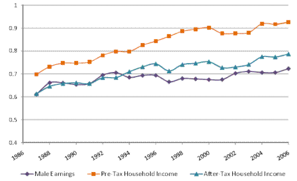
Figure 1b: Cross-Section Variance Gini Coefficient by Year

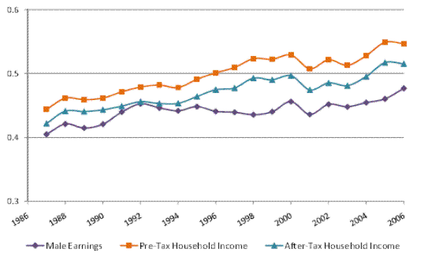Figure 1 Data

Figure 2a: Decomposition of Cross-Sectional Variance: Male Earnings, Baseline Model

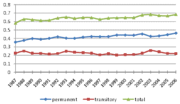
Figure 2b: Decomposition of Cross-Sectional Variance: Male Earnings, Restricted Model 1 (no heterog. profiles)

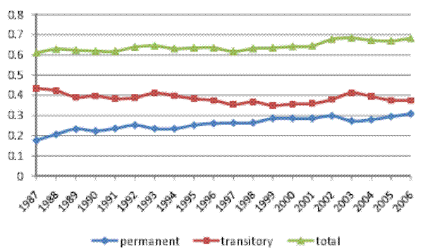
Figure 2c: Decomposition of Cross-Sectional Variance: Male Earnings, Restricted Model 2 (no random walk)

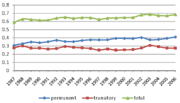
Figure 2c: Decomposition of Cross-Sectional Variance: Male Earnings, Restricted Model 1 (no random walk). See link below for the data underlying this graph.

Figure 2d: Decomposition of Cross-Sectional Variance: Male Earnings, Restricted Model 3 (no MA component)

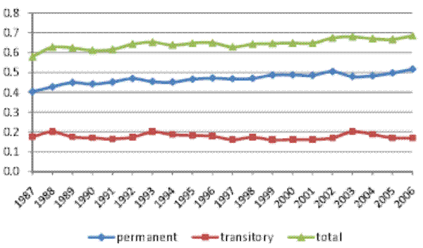Figure 2d: Decomposition of Cross-Sectional Variance: Male Earnings, Restricted Model 1 (no MA component). See link below for the data underlying this graph.

Figure 2 Data

Figure 3a: KSS Decomposition of Cross-Section Variance: Male Earnings

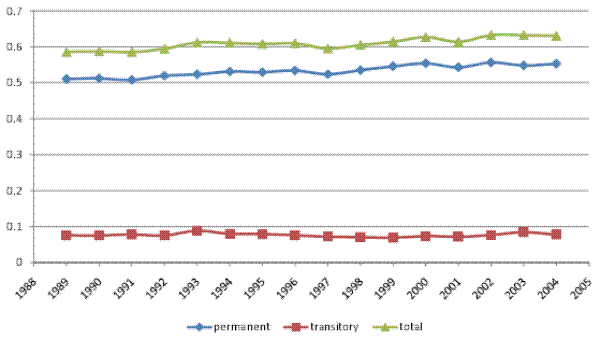
Figure 3b: BPEA Decomposition of Cross-Sectional Variance: Male Earnings

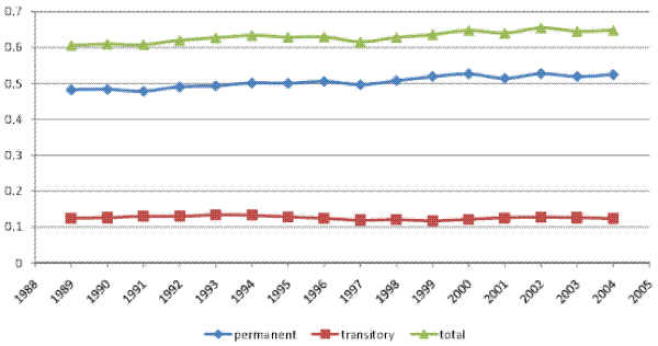Figure 3 Data

Figure 4: Standard Deviation of One-Year and Two-Year Percentage Changes (Volatility): Male Earnings

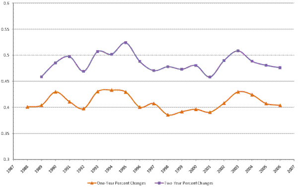Figure 4 Data

Figure 5a: Decomposition of Cross-Section Variance: Pre-tax Household Income, Baseline Model: Male Earnings Sample

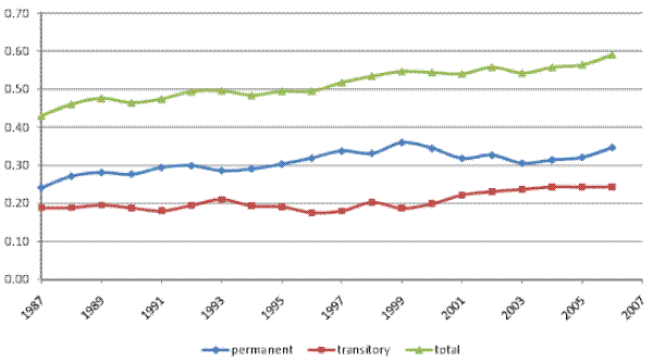
Figure 5b: Decomposition of Cross-Sectional Variance: Pre-Tax Household Income, Restricted Model RM2 (no random walk): Male Earnings Sample

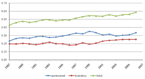Figure 5 Data

Figure 6: Standard Deviation of One-Year and Two-Year Percentage Changes (Volatility): Pre-Tax Household Income: Male Earnings Sample

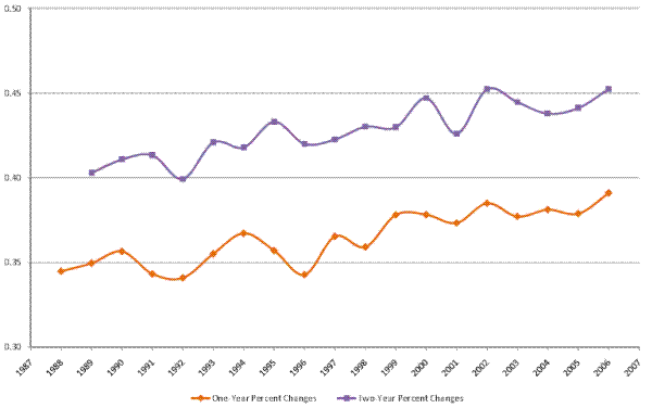Figure 6 Data

Figure 7a: Decomposition of Cross-Section Variance: Pre-tax Household Income, Baseline Model: Full Household Sample

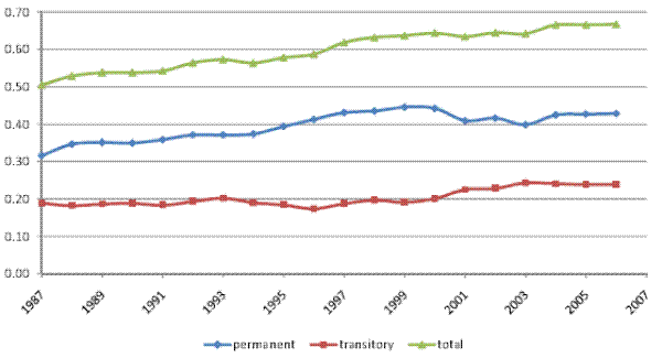
Figure 7b: Decomposition of Cross-Sectional Variance: Pre-Tax Household Income, Restricted Model RM2 (no random walk): Full Household Sample

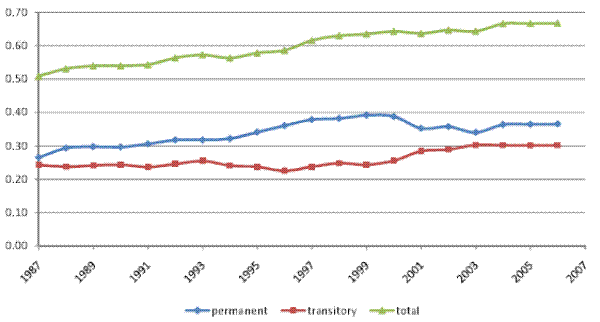Figure 7 Data

Figure 8: Decomposition of Cross-Section Variance: Pre-tax and After-Tax Household Income, Baseline Model: Male Earnings Sample

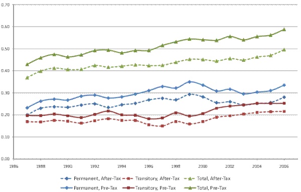Figure 8 Data

Table A.1: Age Distribution by Calendar Year
Year	Male Earnings Sample: Mean	Male Earnings Sample: St Dev	Full Household Income Sample: Mean	Full Household Income Sample: St Dev
1987	39	9.9	40	10.0
1988	39	9.8	40	10.0
1989	39	9.8	40	9.9
1990	39	9.7	40	9.9
1991	39	9.7	40	9.8
1992	40	9.7	40	9.9
1993	40	9.6	40	9.8
1994	40	9.6	40	9.8
1995	40	9.6	40	9.9
1996	40	9.6	40	9.8
1997	40	9.6	41	9.8
1998	40	9.7	41	9.8
1999	41	9.6	41	9.8
2000	41	9.7	41	9.8
2001	41	9.7	41	9.9
2002	41	9.7	41	9.9
2003	41	9.7	42	9.9
2004	41	9.8	42	10.0
2005	41	9.9	42	10.1
2006	41	9.9	42	10.1

Figure A1: Lifecycle Variance Profile of Male Earnings, Controlling for Year Effects: Data, Baseline Model, and Restricted Model 2 (no heterogenous profiles)

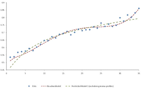Figure A1 Data

Figure A2a: KSS Decomposition of Cross-Sectional Variance, P=3: Male Earnings

Figure A2b: KSS Decomposition of Cross-Sectional Variance, P=7: Male Earnings

Figure A2c: KSS Decomposition of Cross-Sectional Variance, P=9: Male Earnings

Figure A2 Data

Figure A3a: Restricted Model 2 Variance Decomposition: Male Earnings

Figure A3b: Restricted Model 2 Variance Decomposition: Male Earnings + Spousal Earnings

Figure A3a: Restricted Model 2 Variance Decomposition: Male Earnings + Spousal Earnings. See link below for the data underlying this graph.

Figure A3c: Restricted Model 2 Variance Decomposition: Male Earnings + Spousal Earnings + Transfers

Figure A3d: Restricted Model 2 Variance Decomposition: Male Earnings + Spousal Earnings + Transfers + Investment Income

Figure A3e: Restricted Model 2 Variance Decomposition: Total Household Income

Figure A3 Data

Figure A4a: Variance Decomposition, Baseline Model: Male Earnings, DiNardo-Fortin-Lemieux reweighting

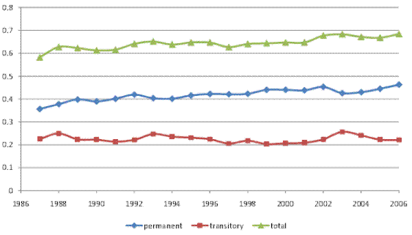
Figure A4b: Variance Decomposition, Restricted Model RM2 (no random walk): Pre-Tax Household Income, Full Household Income Sample, DiNardo-Fortin-Lemieux reweighting

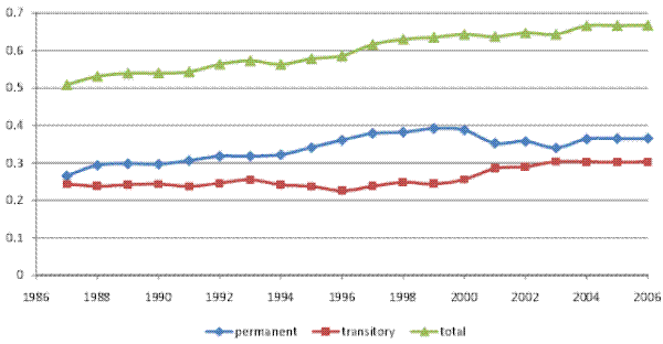Figure A4 Data

Figure A5a: Variance Decomposition, Baseline Model: Male Earnings, Minimum Threshold: One-Half of Full-Year Full-Time Minimum Wage

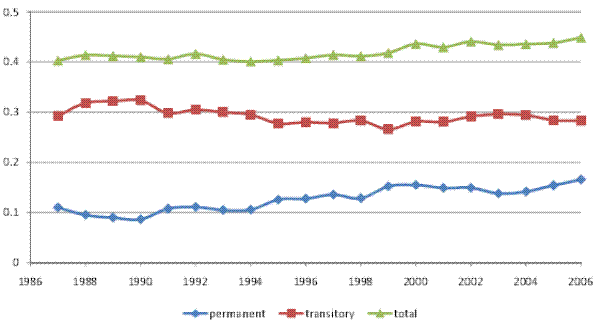
Figure A5b: Variance Decomposition, Restricted Model RM2 (no random walk): Pre-Tax Household Income, Full Income Household Income Sample, Minimum Threshold: One-Half of Full-Year Full-Time Minimum Wage

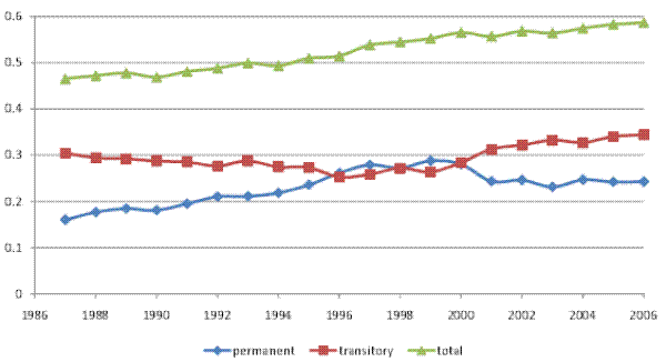Figure A5 Data

Footnotes

* This paper has also been circulated as "Rising Inequality: Transitory or Permanent? New Evidence from a Panel of U.S. Tax Returns 1987-2006". [email protected], [email protected], [email protected], [email protected]. We are grateful to Joe Altonji, Chris Carroll, Eric Engen, Michael Golosov, Michael Palumbo, Dimitris Papanikolaou, Emmanuel Saez, Dan Sichel, and Paul Smith for helpful comments and suggestions. We also thank seminar participants at the Federal Reserve Board, the NBER Summer Institute Consumption group and Labor Studies group, the Federal Reserve Bank of San Francisco, Colegio de Mexico, Bank of Mexico, Bank of Portugal, Applied Micro System Conference at the Federal Reserve Bank of St Louis, the meetings of the European Economic Association and the European Association of Labor Economists, and the U.S. Census Bureau for very constructive discussions. The views presented here are solely those of the authors and do not necessarily represent those of the Treasury Department, the Board of Governors of the Federal Reserve System, or members of their staffs. Return to Text

1. The data are kept at the Treasury Department, and all of our analysis was run at and cleared by the Treasury, in order to maintain the confidentiality of the data. Return to Text

2. We also examine the evolution of measures of dispersion in the distribution of income changes over one and two years (volatility), which provide yet further support for our model-based inequality-trend findings. Return to Text

3. For instance, Kopczuk, Saez, and Song (2010) use longitudinal earnings data from Social Security Administration (SSA) records to document that annual earnings inequality has increased steadily since the early 1950s. See also the earlier contributions by Bound and Johnson (1992); Katz and Murphy (1992); Murphy and Welch (1992); Juhn, Murphy, and Pierce (1993); Katz and Autor (1999); and more recently, Autor, Katz, and Kearney (2008). Return to Text

4. Blundell, Pistaferri, and Preston (2008) find a large increase in the variance of permanent income shocks in the early 1980s, followed by a large increase in the variance of transitory shocks in the late 1980s. However, we cannot directly compare our results with theirs, as our sample periods barely overlap. Return to Text

5. Dynan, Elmendorf, and Sichel (2007) find a continuous increase in the volatility of male earnings in the PSID over the 1967-2004 period. However, their measure of earnings includes income from self-employment, and hence is not directly comparable to ours or to that of the studies mentioned above. Return to Text

6. Guvenen (2007) investigates the differences in the implications of these two specifications of the labor income process for lifecycle consumption behavior. Return to Text

7. Our sample is representative of the U.S. tax filing population. The fraction of U.S. households filing tax returns is generally around 90-95%, see for example Piketty and Saez (2003). Most households who do not file taxes are low-income households. Therefore, our data might miss some changes in income inequality at the bottom of the income distribution. However, we do not view this as a first-order concern, because, as documented by Autor, Katz, and Kearney (2008); and Kopczuk, Saez, and Song (2010), changes in income inequality in the U.S. over our sample period have been concentrated on the upper part of the income distribution. Return to Text

8. The full 1987 stratified random sample actually consisted of two parts, the random sample noted in the text and a high-income oversample. We do not use the high-income oversample in our analysis in this paper. Return to Text

9. On tax returns in which a married couple is filing jointly, the primary filer is the individual listed first on a tax form. This is usually, though not always, the husband. On tax returns of single filers, the primary filer is the individual who filed the return. Return to Text

10. However, taxpayers with one of the two social security number endings who filed as dependents in 1987, or who were listed as a dependent or secondary filer in 1987, were not included in the sample. We discuss this issue in section 3.2. Return to Text

11. However, we have verified the robustness of our results to the exclusion of capital gains from our measure of household income. Return to Text

12. In addition, it is well known that changes in income at low levels of income can unduly affect model estimates. Two commonly used approaches to address this issue are to either exclude or to left-censor low-income observations. Given the issues discussed above, we choose to exclude them. Return to Text

13. This threshold has also been used by Kopczuk, Saez, and Song (2010). In section 8 we check the sensitivity of our results to setting a lower/higher minimum threshold. Return to Text

14. For household income, the figures use our `full' household sample. In our male earnings sample, the cross-sectional variance (of the log) increases by about 40% for both pre-tax and after-tax household income. Return to Text

15. The index

is actually "normalized age" or "potential experience" , defined as

, or years elapsed since age 25. Return to Text

16. The evidence for heterogenous income profiles agrees with the findings of Baker (1997) and Guvenen (2009) on PSID data, and of Baker and Solon (2003) on Canadian tax data. Return to Text

17. In section 8 we examine the robustness of our results to alternative treatments of household size and composition. Return to Text

18. We can also use the estimated model to compute similar decompositions for any age group, or for any age distribution. In fact, we have computed decompositions for several different age groups, but we do not show those results here due to space considerations. Focusing on alternative age distributions leads to similar results. Return to Text

19. Kopczuk, Saez, and Song (2010) use

. They use raw (as opposed to residual) log earnings and restrict observations to individuals who are present in the sample for all five years. We use residual log earnings and do not require individuals to be present in all five years. However, the results are not materially different when we follow their treatment and restrictions. Return to Text

20. At the limit, one would define permanent earnings as average earnings over a person's entire career (say, 35 years), and transitory earnings as the deviation of current earnings from average career earnings. Under this definition, however, it makes little sense to talk about changes over time in the relative importance of a person's permanent income, and it would not be possible to construct a series of such decompositions over time with the available data. Return to Text

21. The difference between the BPEA and the KSS methods essentially reflects a "bias correction term" in the random effects formula upon which the BPEA decomposition is based. For details, see Gottschalk and Moffitt (2009). Return to Text

22. Moffitt and Gottschalk (2008) also favor the use of richer error-components models over the simple BPEA decomposition. Return to Text

23. In particular, for most specifications of an earnings process, volatility and the transitory variance will tend to move together. See the discussion in Shin and Solon (2011) for details on the relation between volatility and transitory variance. Return to Text

24. It also adds some households for which labor earnings of the male primary filer are below the minimum threshold, but for which total household income is above the minimum threshold. Return to Text

25. When using the full household sample, we reject $\sigma _{r}^{2}=0$ . However, in general, the household income data provide less support than male labor earnings for the inclusion of a random walk component in permanent income. In particular, whether or not the restriction $\sigma _{r}^{2}=0$ can be rejected depends on factors such as the specific sample used, the level of the minimum threshold, whether the income data are before or after taxes, and so on. Return to Text

26. Note that the reason why the total variance of household income in Figure V is lower in any given year than the total variance of male earnings shown earlier is that these are variances of residuals, which in the case of household income have removed all variation explained by household size and composition. If we were to compare the raw data instead, the variance of household income would be larger than the variance of male earnings, as seen in Figure I. Return to Text

27. Using the full household income sample, and on average over 1987-2006, male labor earnings account for about 50% of total household income, female labor earnings for 26%, retirement and transfer income for 5%, investment income for 7%, and business income for 12%. Return to Text

28. We analyze increasingly broad income aggregates, rather than individual income categories separately, because, for many households, income from at least some of these individual categories is zero. The large number of zero-income observations makes it difficult to estimate error-components models separately for each income category. Return to Text

29. Investment income here includes capital gains. However, we have verified that excluding capital gains leads to similar conclusions, in that the transitory variance of investment income contributes to the increase in the transitory variance of total household income even if capital gains are excluded. Return to Text

30. Table A.1 of the Appendix shows the mean and standard deviation of the age distribution in each calendar year for both our male earnings sample and our full household sample. Return to Text

31. That is, we define a new sample in which households with different size/composition are treated as separate households. For example, if person A is observed for five years, then person A marries person B and the couple is observed for five years, and then the couple splits and person A is observed for another five years, we treat these three different five-year spells for person A as observations on three different households. Since we are concerned with household income (as opposed to, say, consumption), we focus on the formation and dissolution of couples, and abstract from changes in household size and composition having to do with children. Return to Text

^♣ This version is optimized for use by screen readers. Descriptions for all mathematical expressions are provided in LaTex format. A printable pdf version is available. Return to Text