Monetary-Fiscal Policy Interactions: Interdependent Policy Rule Coefficients
Keywords:
Abstract:
Keywords: Time-varying policy rule coefficients, Monetary and Fiscal policy interactions, Nonlinear state-space models.
JEL Classification Numbers: C11, C32, E63.
1 Introduction
The great recession has raised awareness of the role of monetary-fiscal policy interactions in determining the behavior of economic aggregates. In the United States, for example, reductions in discount and funds rates and even unconventional quantitative easing measures have accompanied fiscal stimulus policies. Moreover, given the high projected fiscal liabilities in developed as well as in some developing countries, interactions are likely to figure more prominently in determining economic outcomes over the coming decades.
The considerations behind monetary-fiscal policy interactions have been part of the monetary and fiscal policymaking literature for a long time. Friedman (1948) proposed a scheme of monetary-fiscal policy interactions to deliver stability in cyclical fluctuations. The seminal work of Sargent and Wallace (1981) provides a formal investigation that illustrates how monetary and fiscal policies interact to determine inflation. The authors show that under fiscal dominance --where a partial monetization of government debt is necessary to avoid default-- the ability of the monetary authority to control inflation disappears. Leeper (1991) examined monetary-fiscal policy interactions within the dynamic stochastic general equilibrium (DSGE) framework. The work of Canzoneri, Cumby and Diba (2010) surveys the positive and normative aspects of monetary-fiscal policy interactions in the existing literature.
Conventionally, there have been two approaches to how each of the policy authorities responds to deviations of its variables of interest from target. One approach specifies a central bank that follows a Taylor (1993) rule under which the nominal interest rate increases more than proportionally when inflation increases. Thus, monetary policy provides the nominal anchor to deliver price-level determinacy. In this approach, the fiscal authority follows a rule under which (lump-sum) taxes stabilize debt. This first approach has been referred to as monetary dominance (see Carlstrom and Fuerst, 2000). We will call it a monetary (M) regime.
The other approach postulates that the fiscal authority does not adjust taxes to stabilize debt. In this case, the central bank cannot stabilize the price level. Thus, fiscal policy provides the nominal anchor for price-level determinacy through expectations about future surpluses, given a level of outstanding nominal liabilities (see Leeper, 1991; Sims, 1994; Woodford, 1994, 1995, 1996; Cochrane, 1998, 2005, 2001). This approach has been referred to as the fiscal theory of the price level. We will call it a fiscal (F) regime.
When the two approaches are considered together, there are four possible combinations of monetary and fiscal policy stances that have been referred to as monetary-fiscal policy interactions. The four combinations are: (i) an M regime; (ii) an F regime; (iii) a regime where no authority provides the nominal anchor and the price level is indeterminate; (iv) a regime where both authorities try to provide the nominal anchor and debt is unbounded.
This paper formulates and solves a New Keynesian model that incorporates monetary and fiscal policy rules whose coefficients are time-varying and interdependent. Time variation and interdependence allow for co-movements in monetary and fiscal policymaking, thereby introducing a direct channel of interactions. This channel influences expectations about future monetary and fiscal policymaking, affecting the dynamics of the variables in equilibrium. In particular, we show that when there are co-movements in monetary and fiscal policymaking in the direction of stable and determinate equilibria --the M and F regimes-- the volatilities of output and inflation are reduced, compared to the case where co-movements in that direction are absent.
As Davig and Leeper (2007) emphasize, policymaking is a complicated process of analyzing and interpreting data, receiving advice, and applying judgment. During some periods policymakers may give more attention to inflation or debt stabilization, while in other periods they may give more attention to output stabilization. Furthermore, a substantial empirical literature argues that policy rules have not remained invariant over the past six decades (see Clarida, Gali and Gertler, 2000; Favero and Monacelli, 2003; Lubik and Schorfheide, 2004; Davig and Leeper, 2006; Fernandez-Villaverde, Guerron and Rubio-Ramirez, 2010;Bianchi, 2012). In this paper, policy rule coefficients move across regimes as functions of exogenous latent factors. In particular, the policy rule coefficients are logistic functions of these latent factors. The logistic function allows the policy rule coefficients to move between two regimes --as with a two-state Markov-switching specification-- with a smooth transition between regimes. We assume that one latent factor influences the evolution of the coefficients of the monetary policy rule and that a different latent factor influences the evolution of the coefficients of the fiscal policy rule.
We introduce interdependence between monetary and fiscal policy by allowing correlation between the two latent factors driving the evolution of the monetary and the fiscal policy rule coefficients. This correlation can be seen as coordination --explicit or implicit-- in policymaking. The correlation between the latent factors allows policy interactions through co-movements in the evolution of the policy rule coefficients.
Given the logistic specification of the policy rule coefficients and the existence of latent factors as additional states, the model is intrinsically nonlinear. We devise a solution method that takes into consideration these nonlinearities. The solution method incorporates agents' expectations on the joint evolution of the policy rule coefficients. This makes the model appropriate to analyze the impacts of monetary and fiscal policies in a framework of interactions.
We employ a limited-information analysis to estimate the policy rule coefficients using Bayesian methods appropriate for nonlinear state-state models. The results indicate that the policy rule coefficients are far from constant. In particular, the monetary policy rule coefficient on inflation switches more frequently than the fiscal policy rule coefficient on debt. There is also a degree of policy interdependence: fiscal policy that focuses on keeping debt under control tends to accompany monetary policy that focuses on keeping inflation under control, and monetary policy that does not increase interest rates actively tends to accompany fiscal policy that does not pay attention to debt increases.
Finally, we calibrate the model to carry out policy analysis. The policy experiments show that contractionary monetary policy can lower inflation, at least in the short-run. The experiments also show that (lump-sum) taxes have effects on output and inflation, as the literature on the fiscal theory of the price level suggests, but the effects are attenuated with respect to a pure fiscal regime.
2 Interactions Between Monetary and Fiscal Policy
In this section, we introduce the concept of interdependence in policymaking that will be central to the analysis of the subsequent sections. We describe the theoretical framework of monetary-fiscal policy interactions and the empirical findings in the literature with respect to policy interactions. Then, we present how we implement interdependence in policymaking through interdependence of the policy rule coefficients.
The theoretical framework of monetary-fiscal policy interactions in a DSGE model was first introduced by Leeper (1991), who shows how different combinations of the magnitudes of monetary and fiscal policy rule coefficients lead to different equilibrium outcomes and local dynamics. Leeper coins the terms "active" and "passive" monetary and fiscal policies to describe how the central bank adjusts interest rates with respect to inflation deviations from target, and how fiscal policy adjusts taxes to changes in public debt. A change more than proportional in nominal interest rates with respect to inflation deviations from target is called "active" monetary policy, while a Ricardian view of fiscal policy, where taxes adjust enough to cover interest payments and to retire debt, is called "passive" fiscal policy. The alternative scenarios with respect to monetary and fiscal policies are called "passive" monetary policy and "active" fiscal policy.1 Leeper finds that the model delivers a bounded unique rational expectations equilibrium as long as monetary policy is active and fiscal policy is passive --regime M-- or if monetary policy is passive and fiscal policy is active --regime F. Also, the model delivers indeterminacy if both monetary policy and fiscal policy are passive, and no bounded solution if both are active. Other papers along this line are Sims (1994) and Leith and Wren-Lewis.
Davig and Leeper (2006) estimate Markov-switching models of monetary and fiscal policy rules with U.S. data. Their results show that there have been numerous switches in monetary and fiscal policy rule coefficients. In particular, whenever the interest rate rule pays more (less) attention to inflation deviations, less (more) weight is given to output deviations. Also, when the tax rule pays more (less) attention to debt deviations, more (less) weight is given to output deviations --in line with an automatic stabilizers argument. These switches deliver the four regimes of policy interactions described above.
Bianchi (2012) conducts a full-information estimation of a Markov-switching DSGE model with policy rule coefficients that switch among three states. The results show that an M regime was in place starting in the 1990s, that an F regime was in place during the 1970s and that a no-bounded-solution regime was in place during the 1980s.
We explicitly introduce co-movements between the coefficients of the monetary and the fiscal policy rules. This setup generalizes the Markov-switching setup in Davig and Leeper (2006) and Bianchi (2012) by introducing interdependence in the evolution of the policy rule coefficients. With this addition, the model allows for a direct channel of interactions in policymaking, so that agents form expectations accordingly, not only in terms of the individual future evolution of policy rule coefficients, but as a framework of joint future policymaking. Below we specify the policy rules, the time variability characteristic of their coefficients, and the way in which we introduce policymaking interdependence.
2.1 Policy Rules
We specify policy rules with coefficients that are time varying. The time-varying coefficients of a particular policy rule are logistic functions of a latent state. More specifically, if ![]() is a time-varying coefficient of a policy rule, it has the following functional form:
is a time-varying coefficient of a policy rule, it has the following functional form:
where
Under this specification, ![]() denotes the lower (upper) bound of
denotes the lower (upper) bound of ![]() , while
, while
![]() denotes its upper (lower) bound (if
denotes its upper (lower) bound (if
![]() ).
).
![]() is a transition coefficient affecting the speed of the transition between the lower and the upper bounds, and
is a transition coefficient affecting the speed of the transition between the lower and the upper bounds, and ![]() is a location parameter determining the value of
is a location parameter determining the value of ![]() at which
at which ![]() crosses the
crosses the ![]() -axis. A graph for
-axis. A graph for
![]() with
with
![]() ,
,
![]() ,
,
![]() , and
, and
![]() is reproduced in Figure 1.
is reproduced in Figure 1.
Two approaches have been proposed in the empirical literature to model time-varying policy rule coefficients. One is a Markov-switching specification with finite number of states (see Davig and Leeper, 2006; Eo, 2009; Davig and Doh, 2009; Bianchi, 2012). The second is a random-coefficient specification (see Kim and Nelson, 2006a; Boivin, 2006; Fernandez-Villaverde et al., 2010). Yksel et al. (2013) offers a survey of the literature on estimation of Taylor rules with time-varying coefficients. An advantage of the Markov-switching specification is that it implies bounded coefficients, which could be important in terms of determinacy and relevance of the equilibrium. With respect to the random-coefficient specification, an advantage is that it implies smooth transitions between states. The logistic specification proposed in this paper generalizes the two approaches: On one hand it allows a policy rule coefficient to switch smoothly from one regime to another, while on the other it allows for a bounded evolution of the coefficient.2
The latent factors can be seen as representing a combination of political and institutional determinants of policymaking. We assume that the latent factors are exogenous with respect to the variables in the model, and that the information that they provide is part of the information set of the agents. That is, agents and policymakers share the same information set. This assumption is needed to solve the model, as will be seen.
2.1.1 Monetary Policy Rule
Monetary policy takes place by means of an interest rate feedback rule of the form
where
where
The time varying monetary policy rule coefficients are denoted by
![]() for inflation deviations from steady state, and
for inflation deviations from steady state, and
![]() for the output gap. Both are logistic functions of the monetary policy latent factor,
for the output gap. Both are logistic functions of the monetary policy latent factor, ![]() .
.
2.1.2 Fiscal Policy Rule
The fiscal rule is a feedback rule for the ratio of lump-sum taxes net of transfers to output,
![]() , of the form
, of the form
where
where
The time-varying fiscal policy rule coefficients are
![]() for debt deviations from steady state and
for debt deviations from steady state and
![]() for the output gap. All are logistic functions of the fiscal policy latent factor,
for the output gap. All are logistic functions of the fiscal policy latent factor, ![]() .
.
2.2 Interdependence in Policymaking
To incorporate direct interactions between policies, we specify the latent factors driving the evolution of the monetary and fiscal policy rule coefficients as follows:
where
In this context, policy authorities react more or less strongly to deviations of their feedback variables from target --inflation and the output gap for the monetary authority, and debt and the output gap for the fiscal authority-- depending on the values of the policy rule coefficients as
driven by the evolution of the latent factors, ![]() and
and ![]() . These latent
factors, ultimately, are going to determine the nature of the possible combinations between monetary and fiscal policymaking. The full specification of the monetary and fiscal policy rule coefficients is as follows:
. These latent
factors, ultimately, are going to determine the nature of the possible combinations between monetary and fiscal policymaking. The full specification of the monetary and fiscal policy rule coefficients is as follows:
A constant-coefficient version of this model delivers an M Regime when
![]() and
and ![]() are sufficiently high --that is, when the monetary
authority reacts strongly to inflation deviations and the fiscal authority reacts strongly to debt deviations. The model delivers an F regime when
are sufficiently high --that is, when the monetary
authority reacts strongly to inflation deviations and the fiscal authority reacts strongly to debt deviations. The model delivers an F regime when
![]() and
and ![]() are sufficiently low --that is, when the fiscal authority
reacts weakly to debt deviations and the monetary authority reacts weakly to inflation deviations. With time-varying coefficients, we can choose values of the parameters defining each of the policy rule coefficients (3)-(6) in a way that the model
delivers determinate equilibria in the long-run with short-run deviations from these equilibria.
are sufficiently low --that is, when the fiscal authority
reacts weakly to debt deviations and the monetary authority reacts weakly to inflation deviations. With time-varying coefficients, we can choose values of the parameters defining each of the policy rule coefficients (3)-(6) in a way that the model
delivers determinate equilibria in the long-run with short-run deviations from these equilibria.
The interactions with long-run determinacy of the equilibria are only well defined if
![]() . In that case, at a given point in time, a high value of
. In that case, at a given point in time, a high value of
![]() --given by a high value of
--given by a high value of ![]() -- is likely to be associated
with a high value of
-- is likely to be associated
with a high value of
![]() --given by a high value of
--given by a high value of ![]() . Also, at a given point in time,
a low value of
. Also, at a given point in time,
a low value of
![]() --given by a low value of
--given by a low value of ![]() -- is likely to be associated
with a low value of
-- is likely to be associated
with a low value of
![]() --given by a low value of
--given by a low value of ![]() . Then,
. Then,
![]() tends to send the economy towards the M and F regimes.
tends to send the economy towards the M and F regimes.
![]() is the case present in the existing literature, where interactions depend on the values of the policy rule coefficients.
is the case present in the existing literature, where interactions depend on the values of the policy rule coefficients.
3 The Model
The economy is populated by a representative household, a final-goods-producing firm, a continuum of intermediate-goods-producing firms, a monetary authority and a fiscal authority. The model extends the setup in An and Schorfheide (2007) to incorporate a fiscal policy rule and time-varying policy rule coefficients. Appendix A details the derivations.
3.1 Households
The representative household derives utility from consumption, ![]() ,4 relative to a habit stock,
,4 relative to a habit stock, ![]() , that is given by the level of technology of the economy, and real money balances,
, that is given by the level of technology of the economy, and real money balances, ![]() ; and derives disutility from working hours,
; and derives disutility from working hours, ![]() . Hence, a representative household chooses consumption, real balances,
bond holdings and working hours to maximize
. Hence, a representative household chooses consumption, real balances,
bond holdings and working hours to maximize
where
given the initial value of nominal assets
3.2 Firms
There are two types of producers: perfectly competitive final goods producers and a continuum of monopolistic intermediate goods producers.
3.2.1 Final Goods Producers
Given the composite good price, ![]() , and intermediate goods prices,
, and intermediate goods prices, ![]() ,
for
,
for
![]() , producers assemble the intermediate goods,
, producers assemble the intermediate goods, ![]() , to obtain a
composite final good,
, to obtain a
composite final good, ![]() , according to a CES technology, so that
, according to a CES technology, so that
where
with
Final good producers choose the demand of intermediate goods, ![]() , to maximize profits given by
, to maximize profits given by
 |
Optimization yields the demand function of intermediate good
Combining (8) and (7) yields the expression of the final good price
 |
3.2.2 Intermediate Goods Producers
Intermediate goods firms produce type ![]() good according to the linear technology
good according to the linear technology
where
where
with
Intermediate good producers face an explicit cost of adjusting their price, measured in units of the finished good, and given by
where
Producers in the intermediate goods sector take wages as given and behave as monopolistic competitors in their goods market, choosing the price for their product taking the demand in (8) as given. Hence, firm ![]() chooses its labor input,
chooses its labor input, ![]() , and its price,
, and its price, ![]() , to maximize
, to maximize
where MRS
3.3 Government
The government finances purchases of goods, ![]() , with a combination of lump-sum taxes,
, with a combination of lump-sum taxes, ![]() , and money creation,
, and money creation,
![]() , so that the implied process for nominal debt,
, so that the implied process for nominal debt, ![]() , satisfies the
budget constraint:
, satisfies the
budget constraint:
given
where
where
3.4 Symmetric Equilibrium
In a symmetric equilibrium, all the intermediate-goods-producing firms make identical decisions, the money supply equals money demand, labor supply equals labor demand, and the net supply of government bonds is zero. Hence, the equilibrium conditions for ![]() are given by
are given by
with
3.5 Frictionless Equilibrium
The frictionless equilibrium is given by the above equilibrium with no frictions (![]() ). Aggregate output in the frictionless equilibrium is given by
). Aggregate output in the frictionless equilibrium is given by
The above is the potential output over which the output gap in the monetary and fiscal policy rules is defined.
3.6 Steady-State Equilibrium
Since technology, ![]() , is a non-stationary process, it introduces a stochastic trend in output, consumption, real money balances, and the real wage. We define the stationary variables as:
, is a non-stationary process, it introduces a stochastic trend in output, consumption, real money balances, and the real wage. We define the stationary variables as:
![]() and
and
![]() . The steady-state equilibrium is the stationary equilibrium in the absence of shocks, and is defined by the following equations:
. The steady-state equilibrium is the stationary equilibrium in the absence of shocks, and is defined by the following equations:
where
3.7 Log-linearized Model and Solution Method
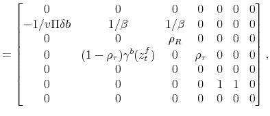
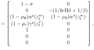
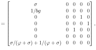
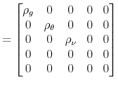
Given that the coefficients of the policy rules are time varying, and the time variation depends on the latent factors, the log-linearization is performed conditioning on the latent factors being at their current values each period. That is the essence of the quasi-linearity of the model. We present the model in log-deviations from the non-stochastic steady state, and show a way to solve it using a method in line with the minimum state variable (MSV) solution approach (McCallum, 1983).
Conditioning on a value of the latent factors at period ![]() ,
, ![]() and
and
![]() , the log-linearized equations characterizing the economy in equilibrium are (
, the log-linearized equations characterizing the economy in equilibrium are (
![]() denotes the log-deviation of variable
denotes the log-deviation of variable ![]() relative to its
non-stochastic steady state,
relative to its
non-stochastic steady state, ![]() ):
):
where
To solve the model, let
![]() ,
,
![]() ,
,
![]() ,
,
![]() ,
,
![]() and rewrite (23)-(32) as
and rewrite (23)-(32) as
where
The proposed solution is given by
where, for
with
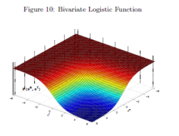
We solve the model using an undetermined coefficients method approach where not only the solution has to be guessed and verified, but also the functional form of the coefficients of the solution. Within the logistic specification of policy rules, the bivariate logistic function (38) satisfies this last requirement. Appendix E shows that the coefficients of the solution indeed follow a bivariate logistic function.
3.8 On Existence, Stability and Uniqueness of the Solution
Existence of the solution is guaranteed by using the undetermined coefficients method. Time-varying coefficients pose a difficulty at guaranteeing stability and/or uniqueness of the solution, in particular if one thinks of stability and/or uniqueness holding in each period of time. The method presented finds a solution that is based on the values of the time-varying policy rule coefficients at their limits, or long-run bounds. These limiting coefficient values are chosen to deliver stability and uniqueness of the solution in a constant-coefficient version of the model, offering well-defined bounds between which the economy evolves and between which agents form expectations. Davig and Leeper (2007) and Farmer et al. (2008) emphasize that stability and uniqueness of Markov-switching rational expectations models have to be discussed within a framework of how agents form expectations about the future evolution of policy rule coefficients, and that is the approach taken at deriving the solution of the model in this paper. Here, we take expectations to the realization of future policy rule coefficients as given by realization of logistic functions of the latent factors.6
4 Estimation Strategy
This section presents the estimation of the policy rules with time-varying coefficients driven by latent factors as specified for the New Keynesian model presented in Section 3. The estimation employs a limited-information estimation approach using Bayesian methods, which
allows obtaining the set of parameters characterizing the policy rules, denoted by
![]() , the set of parameters of the latent factors, denoted by
, the set of parameters of the latent factors, denoted by ![]() ,
and the latent factors themselves.
,
and the latent factors themselves.
4.1 Time-varying Coefficients, Stochastic Volatility and Endogeneity
Let
![]() denote the demeaned nominal federal funds rate in period
denote the demeaned nominal federal funds rate in period ![]() ,
,
![]() the demeaned ratio of federal receipts net of transfers to output in period
the demeaned ratio of federal receipts net of transfers to output in period ![]() ,
,
![]() the demeaned annual inflation rate in period
the demeaned annual inflation rate in period ![]() ,
,
![]() the output gap in period
the output gap in period ![]() and
and
![]() the demeaned average debt to output ratio over the last four quarters. The state-space model is composed of the observation equations
the demeaned average debt to output ratio over the last four quarters. The state-space model is composed of the observation equations
and the transition equations
Assumptions about the distributions of
4.1.1 Stochastic Volatility
The existence of stochastic volatility in the shocks of policy rules with time-varying coefficients has been documented by Davig and Leeper (2006), Fernandez-Villaverde et al. (2010), Bianchi (2012) and Fernandez-Villaverde et al. (2011b),who find that not only switches in policy rule coefficients are detectable in estimation, but also a fair amount of stochastic volatility.7 Hence, the
distribution of the error terms in the policy rules is specified as
![]() and
and
![]() , where
, where
with
In what follows, let
![]() and let the set of parameters of the stochastic volatility processes be denoted
and let the set of parameters of the stochastic volatility processes be denoted ![]() .
.
Equations (43) and (44) are added to the state-space model (39)-(42) to introduce stochastic volatility to the specification of the policy rules with time-varying coefficients.
4.1.2 Endogeneity
Since the work of Clarida et al. (2000), the estimation of monetary policy rules with constant coefficients, in particular the Taylor rule, has taken into account the endogeneity that exists between the shocks of the policy rule and inflation and output. The instrument set used in their GMM estimation contains four lags of: inflation, the output gap, the Federal funds rate, the short-long spread, and commodity price inflation.
With respect to fiscal policy rules with constant coefficients, Li (2009) illustrates the endogeneity/simultaneity problem that arises when estimating a fiscal policy rule like the one presented in this work. In estimating a fiscal policy rule that reacts to contemporary debt and the output gap, Claeys (2008) uses a set of instrumental variables in his GMM estimation that contains lags of: the output gap, debt, unit labor costs, growth in labor productivity, NAIRU, a broad money aggregate, a synthetic interest rate of the EURO area, oil price index, and the SEK/DEM exchange rate.
In terms of estimating linear equations with time-varying coefficients, either in the conventional random-coefficient or Markov-switching setups, Kim (2006) and Kim (2009) establish a Heckman-type two-stage maximum likelihood estimation technique to deal with the endogeneity problem to yield consistent estimates of the hyper-parameters, as well as to provide correct inferences on the time-varying coefficients. Kim and Nelson (2006b) estimate a random coefficients monetary policy rule for the United States using as the set of instruments four lags of: the Federal funds rate, output gap, inflation, commodity price inflation, and M2 growth. In related work, Bae et al. (2011) estimate a Markov-switching coefficients monetary policy rule for the United States using as the set of instruments three lags of: the Federal funds rate, GDP gap, inflation, commodity price changes, and the spread between the long-term bond rate and the three-month Treasury Bill rate.
The set of instruments that we use for both the monetary and the fiscal policy rules is given by four lags of: inflation, the output gap, government spending as proportion of GDP, M2 growth, and commodity price inflation. In a constant-coefficient version of the policy rules, the GMM estimation
obtains the following results with respect to the instrument set: (i) the ![]() test statistics of overidentification restrictions for both of the rules do not reject the null hypothesis that
the instrument set is appropriate at the 5% level of significance; (ii) the exogeneity
test statistics of overidentification restrictions for both of the rules do not reject the null hypothesis that
the instrument set is appropriate at the 5% level of significance; (ii) the exogeneity ![]() test statistics imply that different subsets of instruments are exogenous at the 5% level of
significance; (iii) the Cragg-Donald test statistics reject the null hypothesis of weak instruments at the 5% level of significance for both policy rules. Appendix F describes the setup of the model to correct for endogeneity. Details on the implementation of the Bayesian
estimation of
test statistics imply that different subsets of instruments are exogenous at the 5% level of
significance; (iii) the Cragg-Donald test statistics reject the null hypothesis of weak instruments at the 5% level of significance for both policy rules. Appendix F describes the setup of the model to correct for endogeneity. Details on the implementation of the Bayesian
estimation of ![]() ,
, ![]() ,
, ![]() ,
,
![]() and
and
![]() appear in Appendix H.
appear in Appendix H.
4.2 Data
We use quarterly data from 1960:1 to 2008:3. The sample is not extended beyond 2008:3 to avoid having to deal with the zero lower bound (ZLB) of interest rates. It is still possible to estimate the interdependence between monetary and fiscal policy under the ZLB, but that constitutes a subject of future research. Inflation is the percentage change over the last four quarters of the price level given by the GDP price deflator. The nominal interest rate is the quarterly average of the federal funds rate. The output gap is the log difference between real GDP and the Congressional Budget Office's measure of potential real GDP. M2 growth is the percentage change over the last four quarters of seasonally adjusted M2. Commodity price inflation is the percentage change over the last four quarters of the commodity price index. Government spending is the federal consumption expenditures and gross investment. These variables are obtained from FRED. Lagged debt is the average debt-output ratio over the previous four quarters, where debt is the TreasuryDirect par value of gross marketable federal debt held by the public. Tax net of transfers corresponds to the seasonally adjusted quarterly current receipts of the federal government from which the current transfer payments have been deducted. This variable is obtained from the NIPA Table 3.2.
5 Estimation Results
The choice of prior distributions, hyper parameters, means of ![]() draws from the posterior distribution after trimming the first
draws from the posterior distribution after trimming the first ![]() out of
out of ![]() draws and thinning every 200th draw, along with 90% confidence sets appear in Table 1.8 In order to keep the estimation relatively simple, we impose two restrictions that do not change the results qualitatively: First, we
assume that the output gap coefficients of both policy rules are not time varying, which allows us to focus on capturing the interdependence between monetary and fiscal policy making in terms of the co-movement of the Taylor rule coefficient of inflation and the tax rule coefficient of lagged debt.
Second, we assume that the location parameters of the logistic policy rule coefficients,
draws and thinning every 200th draw, along with 90% confidence sets appear in Table 1.8 In order to keep the estimation relatively simple, we impose two restrictions that do not change the results qualitatively: First, we
assume that the output gap coefficients of both policy rules are not time varying, which allows us to focus on capturing the interdependence between monetary and fiscal policy making in terms of the co-movement of the Taylor rule coefficient of inflation and the tax rule coefficient of lagged debt.
Second, we assume that the location parameters of the logistic policy rule coefficients,
![]() and
and
![]() , are zero.
, are zero.
| Parameters | Prior:Density | Prior: Mean | Prior: SD | Posterior:Mean | Posterior: 90% Conf. Set |
|
|
Gamma | 0.8 | 0.2 | 0.57 | [0.35, 0.84] |
|
|
Gamma | 1.2 | 0.3 | 1.06 | [0.61, 1.68] |
|
|
Gamma | 10 | 8 | 5.05 | [0.10, 15.72] |
| Gamma | 0.5 | 0.4 | 0.25 | [0.08, 0.52] | |
| Beta | 0.9 | 0.05 | 0.96 | [0.91, 0.99] | |
|
|
Normal | -0.02 | 0.05 | 0.00 | [-0.06, 0.06] |
|
|
Gamma | 0.1 | 0.05 | 0.09 | [0.03, 0.20] |
|
|
Gamma | 10 | 8 | 4.03 | [0.04, 14.70] |
| Gamma | 0.5 | 0.4 | 0.76 | [0.44, 1.16] | |
| Beta | 0.9 | 0.05 | 0.94 | [0.93, 0.96] | |
|
|
Beta | 0.9 | 0.05 | 0.86 | [0.74, 0.95] |
|
|
Beta | 0.9 | 0.05 | 0.88 | [0.78, 0.95] |
| Normal | 0 | 2 | -0.41 | [-2.66, 1.93] | |
| Normal | 0 | 2 | 0.05 | [-2.26, 2.35] | |
| -- | 0.20 | [0.02, 0.47] | |||
|
|
-- | -2.05 | [-2.41, -1.70] | ||
|
|
-- | 0.77 | [0.63, 0.90] | ||
| -- | 0.57 | [0.39, 0.78] | |||
|
|
-- | -2.93 | [-5.18, -0.68] | ||
|
|
-- | -1.15 | [-1.45, -0.89] | ||
|
|
-- | 0.48 | [0.27, 0.64] | ||
| -- | 0.88 | [0.65, 1.11] | |||
|
|
-- | -5.85 | [-12.48, 0.59] |
- -- denotes a flat prior.
Figure 2 shows that the estimated model does acceptably well at explaining the observed time series of interest and tax rates.
5.1 Choice of Prior Distributions
With respect to the monetary policy rule coefficients, there exist results in the literature about the values that they take in different regimes. Clarida et al. (2000) estimate that the inflation coefficient is 0.83 in the pre-Volcker era and 2.15 in the Volcker-Greenspan era. Lubik and Schorfheide (2004) find that the coefficient on inflation is estimated at 0.77 or 0.89, depending on the prior used, in the pre-1982 era, and 2.19 in the post-1982 era. Bianchi (2012) finds that the coefficient on inflation is estimated to be 0.94, 1.25, or 1.6 in a three-regime Markov-switching specification. Davig and Leeper (2011) find that the inflation coefficient switches between 0.53 and 1.29. We specify the prior distribution that characterizes the lower bound of the inflation coefficient with a mean of 0.8, and the upper bound with a prior distribution whose mean is 2 (the sum of 0.8 and 1.2 in Table 1). In regard to the fiscal policy rule coefficients, Bianchi (2012) finds that the coefficient on debt is estimated to be 0.0006, -0.0007, or -0.0036. Davig and Leeper (2011) estimate that the coefficient on debt switches between -0.025 and 0.071. We set the prior mean of the lower bound of the debt coefficient to -0.02, and the mean of the prior distribution that sets the upper bound of the coefficient to 0.08 (the sum of -0.02 and 0.1 in Table 1). The policy rule coefficients on the output gap for both policy rules have 0.5 as the prior mean.
The prior distribution specification of the transition coefficients of both logistic policy rule coefficients is set to have a mean of 10 with a standard deviation of 8. We recall that the larger the coefficient is, the more rapid the transition between states is. Values of the coefficient greater than 10 imply a specification that mimics closely a Markov-switching-like transition. The choice of this prior distribution allows the coefficient to take low or high values.
The smoothing coefficients of the policy rules have prior distributions that are standard in terms of the persistence that they represent for interest and tax rates in the data.
A coefficient that deserves attention is the correlation coefficient between the shocks of the latent factors, which determines the degree of interdependence between monetary and fiscal policymaking. The prior distribution chosen is uniform on [0,1]. We recall that a positive value of this parameter implies that monetary and fiscal policy co-move in such a way that they tend to deliver outcomes in the M or the F regime more frequently than outcomes in the indeterminacy or no solution regimes. Hence, by choosing a prior distribution on the nonnegative domain, we are imposing a model with either co-movements towards the determinate regimes or absence of co-movements in that direction, but we are not allowing co-movements in the direction of the indeterminate or unbounded debt regimes.
Finally, following Fernandez-Villaverde et al. (2011a), we do not specify prior distributions for the parameters of the stochastic volatility processes.
5.2 Parameter Estimates
The estimated parameters of the monetary and fiscal policy rule coefficients in Table 1 have the expected magnitudes and signs. In particular, for the monetary policy rule, the inflation coefficient takes values in (0.57, 1.63), while the output gap coefficient has a posterior mean of 0.25. With respect to the fiscal policy rule, the debt coefficient takes on values in (0.001, 0.095), while the output gap coefficient has a posterior mean of 0.76. The speed of transition of the policy rule coefficients is estimated to be higher for the inflation coefficient of the monetary policy rule than for the debt coefficient of the tax rule. This implies that the fiscal authority has a slower transition across states (in terms of how taxes react with respect to deviations of debt) than the monetary authority does (in terms of how the interest rate reacts with respect to inflation). This result is consistent with the legislative and implementation lags of fiscal policymaking.
The latent factors show relatively high persistence, with the fiscal policy latent factor being somewhat more persistent than the monetary policy one. This result implies that fiscal policy regimes are likely to last longer than monetary policy regimes.
Finally, the correlation between the latent factors has an estimated posterior mean of 0.20 and a 90% confidence set given by (0.01, 0.47). This result implies that there is a degree of direct interactions between policies. In particular, monetary tightenings to stabilize inflation tend to be accompanied by fiscal policy that stabilizes debt (M regime), while fiscal policy that departs from debt stabilization tends to be accompanied by interest rates that react weakly to inflation (F regime).
5.3 Evolution of Policy Rule Coefficients
Figure 3 shows the smoothed estimates of the monetary policy rule coefficient for inflation on the left axis, and of the fiscal policy rule coefficient for debt on the right axis. Two facts are apparent from this figure: First, the fiscal policy rule coefficient on debt was low during most of the 1970s, the second half of the 1980s, and the first half of the 1990s. Second, the monetary policy rule coefficient on inflation was high during the second half of the 1960s
and the first half of the 1970s, during the first half of the 1980s, and during the first half of the 2000s. In the next paragraphs, we discuss the evolution of each of the policy rule coefficients to compare the econometric results with the narrative about monetary and fiscal policymaking and with similar results in the literature.The evolution of the monetary policy rule coefficient on inflation reveals that the Federal Reserve conducted a hawkish monetary policy during the second half of 1960s, as Davig and Leeper (2011), Bianchi (2010), Eo (2009) and Fernandez - Villaverde et al. (2010) find, with a tendency to ease it towards the end of the decade. During the mid 1970s the interest rate did not react strongly to inflation. Most studies in the literature find a passive monetary policy during this decade, except Bolvin (2006), who finds that monetary policy was tight during the first half of the 1970s. At the end of the 1970s monetary policy switched rapidly to a hawkish regime. This switch in policymaking is also found by Davig and Doh (2009), Eo (2009) and Bianchi (2010) who find, based on estimations of Markov-switching policy rule coefficients, that the active monetary policy periods started around, or a little earlier than, the mid 1980s. The graph shows that monetary policy continued to be relatively hawkish during most of the 1980s. Starting in the late 1980s, the estimates of the model suggest a relatively weak response to inflation, which lasted through much of the 1990s. A study that finds a similar result is Fernandez-Villaverde et al. (2010).9 In 2000s, monetary policy increased its reaction to inflation until 2005 and then the strength of the reaction declined. The empirical evidence is divided with respect to this result: On one hand Eo (2009), Davig and Doh (2009) and Bianchi (2010) find that monetary policy was actively fighting inflation, while on another Fernandez-Villaverde et al. (2010) and Davig and Leeper (2011) find the opposite.
For a narrative perspective on the results, we rely on the history of the monetary policy of the Federal Reserve as told by Hetzel (2008). He compares Fed Chairman William Martin to Fed Chairman Paul Volcker and Fed Chairman Alan Greenspan in that Martin believed that raising short-term interest rates in an expansion was a way to preempt inflation. That allows to understand the behavior of monetary policy, according to the graph, during the second half of the 1960s. Hetzel also mentions the weak reaction of interest rates to inflation during the 1970s due to the focus of the central bank to promote employment and the belief that inflation was a nonmonetary phenomenon. According to Hetzel, the 1980s saw the commitment of the Federal Reserve to money targets allowing the FOMC to raise interest rates by whatever extent necessary to lower inflation. The results show that the reaction coefficient of the interest rate to inflation was indeed relatively high.
After tightening monetary policy at the end of the 1980s to counteract concerns about inflation, the results show a decline in the reaction of the federal funds rate to inflation at the beginning of the 1990s to help with the recovery after the recession. With inflation declining during this decade and interest rates remaining nearly flat, except for the rise between 1993 and 1995 due to the "1994 inflation scare" (see Hetzel (2008) ), the reaction coefficient on inflation declines until the events of the Asian and Russian crises. During 1998 the Federal Reserve moved the interest rate in the same direction as declining inflation, causing a spike in the evolution of the inflation coefficient. In the 2000s, with declining inflation and interest rates between 2001 and the beginning of 2003, the reaction coefficient to inflation rises rapidly to reach a peak in the second quarter of 2003 when concerns about interest rates being close to the zero-bound arose for the first time. With inflation stable and interest rates rising during 2004, the reaction coefficient declines. Then the coefficient rises at the end of the sample, between 2005 and 2008, reflecting interest rates that risen more than what inflation risen during the period.
For the debt policy rule coefficient, the results show a coefficient responding weakly to lagged debt during the 1970s, a result mostly in the same lines as those in Davig and Leeper (2006), Bianchi (2012), and Favero and Monacelli (2003). The results also show a low debt coefficient during the second half of the 1980s and the first half of the 1990s, a result that is compatible with the findings in Bianchi (2012).
In terms of the narrative, the tax reductions in the revenue act of 1964 can help understand the decline of the coefficient during the 1960s, while the revenue and expenditure control act of 1968 and the tax reform act of 1969 can help explain the rise of the coefficient at the end of the decade. The subsequent tax reforms of 1971, 1975 and 1976 help explain the decline in the debt coefficient during the 1970s. The rise of the coefficient observed at the end of the decade has to do with the fact that the debt-GDP ratio rises between 1975 and 1980, inclusive, and the net revenue-GDP ratio rose in that period. That relationship breaks up during the 1980s due to the tax reforms of the decade, in particular the recovery tax act of 1981. During the 1990s, the coefficient rises rapidly, most likely due to the changes implemented in the budget reconciliation act of 1993. The taxpayer relief act of 1997 can help understand the decline in the coefficient at the end of the decade. The decline of the debt coefficient in the 2000s can be attributed to the tax relief acts of 2001 and 2003, and the subsequent stimulus acts of 2004 and 2008.
In a historical perspective, the evolution of the estimated policy rule coefficients suggest
that policy leaned towards a fiscal regime during some part of the 1970s, a result emphasized by Bianchi (2012). On the other hand, the estimates favored a monetary regime during the second half of the 1960s, the first half of the 1980s, and the first half of the 2000s. The macroeconomic model allows short-run dynamics that visit temporarily all the regimes, including the indeterminate and the no-bounded-solution regimes, but the long-run expectations of a mixed regime imply dynamics that tend to move the economy between the two determinate regimes.5.4 Evolution of Estimated Stochastic Volatilities
Figure 4 shows the evolution of the estimated stochastic volatilities for the interest and tax rate rules. The estimation shows that the volatility of interest rates was significantly higher during the beginning of the 1980s due to the important change in
conducting monetary policy. Also, volatility is somewhat lower starting in the 1990s, a phenomenon referred to as the great moderation (see Stock and Watson, 2002), and stays low with a small peak at the end of the sample period when the great recession hit. On the other hand,
fiscal policy volatility shows spikes in the mid 1970s, the first half of the 2000s, and the beginning of the great recession. All these events are associated with some kind of fiscal stimulus. It is worth noting that the persistence of the volatility of monetary policymaking, given by the
estimated coefficient
![]() , is higher than the persistence of the volatility of fiscal policymaking, given by the estimated coefficient
, is higher than the persistence of the volatility of fiscal policymaking, given by the estimated coefficient
![]() , as can be seen in Table 1.
, as can be seen in Table 1.
6 Monetary and Fiscal Policy Analysis
This section presents the results of monetary and fiscal policy experiments through impulse-response functions. The section also presents the effect of policy interdependence in reducing the volatility of output and inflation.
6.1 Nonlinear Impulse Response Analysis
We perform policy experiments with the model solved using the proposed solution method and calibrated according to the estimated parameters of the policy rule coefficients. Since the estimation is not constrained to deliver a continuous solution to the macroeconomic model as presented in
Appendix E, we calibrate the model with coefficients that are consistent with continuity of the solution. In particular, we calibrate the lower bound of the monetary policy rule coefficient on inflation,
![]() , to be 0.85 instead of 0.57. The fiscal policy rule coefficients,
, to be 0.85 instead of 0.57. The fiscal policy rule coefficients,
![]() and
and
![]() , are calibrated to 0.03 and 0.07 instead of 0 and 0.09, respectively.
, are calibrated to 0.03 and 0.07 instead of 0 and 0.09, respectively.
For the markup in steady state and the price adjustment cost parameter, Keen and Wang (2007) show that, given a steady state markup and a fraction of firms that re-optimize each period, there is a corresponding value for the price adjustment cost parameter. We set the markup to
20% and the fraction of re-optimizing firms to 25% each period (a firm re-optimizes every 12 months). These values correspond, approximately, to
![]() and
and ![]() . Other parameters that need to be specified are:
. Other parameters that need to be specified are:
![]() , the steady state gross quarterly rate of output growth, which is set to 1.0081 , the average over the sample period that implies a steady state annual growth rate of approximately 3.25%;
, the steady state gross quarterly rate of output growth, which is set to 1.0081 , the average over the sample period that implies a steady state annual growth rate of approximately 3.25%; ![]() , the steady state gross quarterly rate of price
inflation, which is set to 1.0084 , the average over the sample period that implies a steady state annual inflation of approximately 3.4%;
, the steady state gross quarterly rate of price
inflation, which is set to 1.0084 , the average over the sample period that implies a steady state annual inflation of approximately 3.4%; ![]() , the steady state level of debt to output, which is set to 0.3354, the average over the sample period;
, the steady state level of debt to output, which is set to 0.3354, the average over the sample period; ![]() , the ratio of
government spending to output is set to 0.081, also the average over the sample period;
, the ratio of
government spending to output is set to 0.081, also the average over the sample period; ![]() , the ratio of outstanding money balances to debt, is set to 0.2 following Kim (2003);
, the ratio of outstanding money balances to debt, is set to 0.2 following Kim (2003); ![]() is set to 0.99;
is set to 0.99; ![]() is set to 1; and
is set to 1; and
![]() is set to 1, so that the Frisch elasticity of labor supply is unity.
is set to 1, so that the Frisch elasticity of labor supply is unity.
We perform two policy experiments. First, a one-time i.i.d shock on the interest rate. Second, a one-time i.i.d shock on the tax-to-output ratio. The responses to these shocks are calculated under three scenarios: starting at regime M and staying there forever, starting at regime F and staying there forever, and a Mixed regime.
In the Mixed regime, the latent factors start at their means, which we set to zero according to the confidence sets in Table 1. These zero values imply corresponding values for the initial monetary and fiscal policy rule coefficients (
![]() and
and
![]() ). Over the response horizon, the policy rule coefficients evolve according to their logistic specifications and the joint evolution of the latent factors. To compute
the responses in the Mixed regime, we take the average of the responses for given realizations of the policy rule coefficients. Note that in the Mixed regime the initial values of the policy rule coefficients imply that the economy is in regime M. However, because agents expect regime F to take
place for some time in the future, the dynamics of the Mixed regime are not those of a pure M regime, but of a regime that incorporates the features of both regimes M and F.
). Over the response horizon, the policy rule coefficients evolve according to their logistic specifications and the joint evolution of the latent factors. To compute
the responses in the Mixed regime, we take the average of the responses for given realizations of the policy rule coefficients. Note that in the Mixed regime the initial values of the policy rule coefficients imply that the economy is in regime M. However, because agents expect regime F to take
place for some time in the future, the dynamics of the Mixed regime are not those of a pure M regime, but of a regime that incorporates the features of both regimes M and F.
6.1.1 A Monetary Contraction
Figure 5 shows the responses of some of the variables of the model to a one-time 25 basis point i.i.d. shock on the interest rate.
The effects of a monetary contraction in a New Keynesian model in regime M are well known: an open market operation that sells debt to households, and that is expected to be corrected in the future via higher taxes, does not change household wealth and only increases the nominal interest rate. With sticky prices the real interest rate increases, reducing consumption, output and inflation. As the nominal interest rate decreases, as well as the real interest rate, the output gap returns to zero and inflation to its steady state. Taxes first decrease due to feedback from the output gap and then increase due to their Ricardian response to lagged debt, which is now higher. Given the persistence of taxes, the present value of expected future surpluses increases and slowly returns to steady state, while the present value of expected future seignorage decreases on impact.
In regime F, an open market operation that sells debt to households, which is not expected to be corrected in the future via higher taxes, increases household's wealth. The increase in wealth attenuates the liquidity-induced contraction in demand. Inflation drops on impact given that the liquidity effect dominates the wealth effect.10 The real interest rate increases on impact, causing output to fall. Note that a "price puzzle", in the sense of Sims (1992), is present. Over the response horizon, inflation increases due to some unpleasant monetarist arithmetic: Taxes are not expected to increase to pay back the debt and some monetization of the deficit is expected. Taxes decrease on impact, reacting mainly to the output gap, and then increase above steady state due to the initial increase in debt, since the debt coefficient of the fiscal policy rule is small but positive. Given the persistence of taxes, the tax increase above steady state makes the present value of expected future surpluses increase on impact.
In the Mixed regime, agents compute their responses based on their expectation of the evolution of future regimes. As a result, the effects of a monetary contraction on inflation and output are between the two previously described regimes. Agents' expectations incorporate the behavior of the economy under both regimes M and F. Thus, there is lower inflation on impact and there is a wealth effect that translates into marginally higher inflation in the long run. Output also falls on impact due to higher real interest rates. These results mean that, as long as the economy does not start at one of the limiting regimes and stays there forever, some of the wealth effect derived from regime F will influence the economy's response to a monetary contraction. That is, a monetary contraction decreases inflation on impact, but the long-run effect is an increase of inflation above steady state. Sims (2011) describes this feature of monetary policy as "stepping on a rake".
The impact response of inflation and output to a 25 basis points increase in the interest rate is shown in Figure 7 for a combination of values of
![]() and
and
![]() for
for ![]() in [-10,10]. The responses of inflation and output
range from -1.03% and -1.37%, respectively, in regime M (
in [-10,10]. The responses of inflation and output
range from -1.03% and -1.37%, respectively, in regime M (
![]() ), to -0.15% and -0.42%, respectively, in regime F (
), to -0.15% and -0.42%, respectively, in regime F (
![]() ). In between these limits there exists a continuum of impact responses given by the possible combinations of the monetary and fiscal policy rule coefficients. Hence, the
size of the impact response of inflation and output to a monetary policy shock will depend on the state of the
). In between these limits there exists a continuum of impact responses given by the possible combinations of the monetary and fiscal policy rule coefficients. Hence, the
size of the impact response of inflation and output to a monetary policy shock will depend on the state of the
6.1.2 A Fiscal Contraction - Tax increase
Figure 6 shows the responses of some of the variables of the model to a one-time 100 basis point i.i.d shock on the tax-to-output ratio.
In regime M, a tax increase that retires debt does not have any effect on output or inflation due to the Ricardian nature of the equilibrium: higher taxes today are expected to be fully compensated with lower taxes in the future, with no wealth effect on households. Wealth is unchanged because, on impact, the present value of expected future surpluses and seignorage are unchanged. Taxes decrease after impact in reaction to the reduction in debt and, given the persistence of taxes, remain below steady state at long horizons. Debt falls, anticipating the decrease in the present value of expected future surpluses. There are no changes in seignorage.
A tax increase in regime F reduces wealth since the increase is not expected to be reversed in the future. The decrease in wealth reduces demand for goods and, hence, inflation. Since the nominal interest rate responds passively to changes in inflation, the real interest rate increases, reducing consumption and output. The present value of expected future surpluses increases due to persistently higher taxes that will not be compensated for in the future. The present value of expected future seignorage declines on impact due to lower inflation and interest rates. Overall, the change in the expected present value of government net receipts implies that debt initially increases before returning to steady state.
In the Mixed regime, as with the monetary contraction, agents' behavior is based on their expectation of the evolution of future regimes. As a result, the effects of a fiscal contraction are between the two previously described regimes. That is, a change in taxes has effects on inflation and output due to the wealth effect that emerges because agents do not expect the
initial increase in taxes to be completely reversed in the future. However, the effects are attenuated with respect to a pure F regime.The impact response of inflation and output to a 100 basis point increase in the tax-to-output ratio is shown in Figure 8 for a combination of values of
![]() and
and
![]() for
for ![]() in [-10,10]. The responses of inflation and output
range from 0% and 0%, respectively, in regime M (
in [-10,10]. The responses of inflation and output
range from 0% and 0%, respectively, in regime M (
![]() ), to -0.71% and -0.78%, respectively, in regime F (
), to -0.71% and -0.78%, respectively, in regime F (
![]() ). In between these limits there exists a continuum of impact responses dependent on the combinations of monetary and fiscal policy rule coefficients. Hence, the magnitude
of the impact responses of inflation and output to a fiscal policy shock will depend on the state of the monetary and fiscal policy rule coefficients at the time of policy implementation.
). In between these limits there exists a continuum of impact responses dependent on the combinations of monetary and fiscal policy rule coefficients. Hence, the magnitude
of the impact responses of inflation and output to a fiscal policy shock will depend on the state of the monetary and fiscal policy rule coefficients at the time of policy implementation.
6.2 Policy Interdependence: Its Effects
In this section we analyze the effect of interdependence in monetary and fiscal policy making as measured by a positive correlation coefficient between the latent factors, ![]() . In
Section 5.2, we showed that the estimated posterior mean of the correlation coefficient between the latent factors is 0.2. As mentioned previously, this value implies that monetary tightenings to stabilize inflation tend to be accompanied by fiscal policy that
stabilizes debt (regime M) while fiscal policy that deviates from debt stabilization tends to be accompanied by a loose monetary policy that contributes to keep debt stable (regime F).
. In
Section 5.2, we showed that the estimated posterior mean of the correlation coefficient between the latent factors is 0.2. As mentioned previously, this value implies that monetary tightenings to stabilize inflation tend to be accompanied by fiscal policy that
stabilizes debt (regime M) while fiscal policy that deviates from debt stabilization tends to be accompanied by a loose monetary policy that contributes to keep debt stable (regime F).
The existing literature on Markov-switching policy rule coefficients assumes that independent states drive the switches between regimes of the coefficients of each policy rule. In that sense, there are not explicit interactions between monetary and fiscal policymaking. In the context of the
current paper, that would be analogous to the case where
![]() .
.
To examine the effect of policy interdependence (
![]() ), we solve and simulate the model for different values of the correlation coefficient between the latent factors. We simulate the
), we solve and simulate the model for different values of the correlation coefficient between the latent factors. We simulate the
As can be seen from the figure, the stronger the association between monetary and fiscal policymaking, as measured by the degree of synchronization of changes in the coefficients of the policy rules, the smaller the unconditional standard deviation of the series. The results show that going from
a scenario of independent switching in the coefficients of the policy rules to a scenario of relatively low interdependence, as measured by
![]() , would result in a decrease of between 1% and 2% in the unconditional standard deviation of inflation or output.
, would result in a decrease of between 1% and 2% in the unconditional standard deviation of inflation or output.
To understand this result, recall that the only two determinate equilibria arise in regimes M and F, while the other two equilibria imply either an indeterminacy or a solution with unbounded debt. Under the indeterminate equilibrium, the presence of sunspot shocks may imply a higher volatility of inflation, whereas under the unbounded debt equilibrium there is not a stationary solution to the macroeconomic model. Hence, policy co-movements in the direction of the M and F regimes would help stabilize output and inflation with respect to the case of no policy co-movements or co-movements away from determinate regimes.
7 Concluding Remarks
In this paper, we formulated and solved a New Keynesian model with time-varying policy rule coefficients that allows for interdependence between monetary and fiscal policymaking. This specification permits analyzing the effects of monetary and fiscal policy in an environment where agents expect the economy to evolve between times where the nominal anchor is provided by monetary policymaking and times where the nominal anchor is provided by fiscal policymaking.
We estimated the policy rules, and obtained results showing that there have been fluctuations in the monetary and fiscal policy rule coefficients. Additionally, policymaking shows important persistence, with fiscal policy being somewhat more persistent than monetary policy. The results also show that there is a degree of policy interdependence, given by a positive correlation coefficient between the latent factors that drive the evolution of policy rule coefficients. More specifically, fiscal policy that focuses on keeping debt under control tends to accompany monetary policy that focuses on keeping inflation under control, and monetary policy that keeps interest rates with a low reaction to inflation tends to accompany fiscal policy that departs from debt stabilization.
Policy experiments show that when agents expect the economy to evolve between a regime of monetary price determination and a regime of fiscal price determination, contractionary monetary policy lowers inflation in the short run and increases it in the long run. The experiments reveal that (lump-sum) taxes have effects on output and inflation, as the literature on the fiscal theory of the price level suggests, but effects are attenuated relative to a pure fiscal regime.
A. Model Setup
The representative household solves the following problem:
 |
subject to
 |
||
 given given |
||
 |
where
where
From (45) and (46)
From (45), (47) and (48),
Profits of intermediate firm ![]() are given by
are given by
Substituting (8) and (9) in (53) yields
![\displaystyle \frac{D_t(j)}{P_t} = \left[ \left(\frac{P_t(j)}{P_t}\right)^{1-\theta_t} - \psi_t \left(\frac{P_t(j)}{P_t}\right)^{-\theta_t} - \frac{\phi}{2}\left( \frac{P_t(j)}{\Pi P_{t-1}(j) }-1 \right)^2\right]Y_t.](img335.gif) |
Then, intermediate firm
 MRS MRS![\displaystyle _{t,t+k} \left[ \left(\frac{P_t(j)}{P_t}\right)^{1-\theta_t} - \psi_t \left(\frac{P_t(j)}{P_t}\right)^{-\theta_t} - \frac{\phi}{2}\left( \frac{P_t(j)}{\Pi P_{t-1}(j) }-1 \right)^2\right]Y_t.](img337.gif) |
The first order condition to this maximization problem is
In a symmetric equilibrium,
![]() ,
,
![]() and
and
![]() , hence
, hence
In equilibrium,
![]() ,
, ![]() and
and ![]() . Then, (11), (55) and (49) imply (12). In the symmetric equilibrium, substituting (45) into (54) yields (13). Finally, the symmetric equilibrium yields (15), (52) is (16), and (50) is (14).
. Then, (11), (55) and (49) imply (12). In the symmetric equilibrium, substituting (45) into (54) yields (13). Finally, the symmetric equilibrium yields (15), (52) is (16), and (50) is (14).
Before proceeding to the log-linearization of the model, it is convenient to write (11) in terms of nominal output. The resulting expression is
where
To obtain (17), start with (15) and recall the definition of
![]() to get
to get
 |
In the symmetric equilibrium, from (9),
 |
Once the variables have been de-trended by dividing them by ![]() , the absence of shocks yields (18) from (14), (21) from
(16), (19) from combining (12) and (17), (20) from (19) and
, the absence of shocks yields (18) from (14), (21) from
(16), (19) from combining (12) and (17), (20) from (19) and
![]() , and (22) from (56) with
, and (22) from (56) with
![]() .
.
C. Obtaining the Coefficients of the Logistic Functions
Each of the elements in the matrices
![]() have the bivariate logistic functional form (38), which is reproduced here for convenience and is
illustrated in Figure 10:
have the bivariate logistic functional form (38), which is reproduced here for convenience and is
illustrated in Figure 10:

|
To avoid computational costs, we find the solutions to the coefficients in
![]() and
and
![]() only, solving for inflation and output, leaving the full solution of the model to be accounted for the structural equations of the state variables (25)-(32). Given the structure of the vector of shocks,
only, solving for inflation and output, leaving the full solution of the model to be accounted for the structural equations of the state variables (25)-(32). Given the structure of the vector of shocks,
![]() is a matrix with 10 distinct elements. Given the structure of the vector of state variables,
is a matrix with 10 distinct elements. Given the structure of the vector of state variables,
![]() is a matrix with 10 distinct elements as well, although it has 14 entries. Therefore, in total there are
is a matrix with 10 distinct elements as well, although it has 14 entries. Therefore, in total there are
![]() coefficients of the logistic functions to be found to obtain a solution.
coefficients of the logistic functions to be found to obtain a solution.
C.1 Finding  and
and 
Notice that the time-varying policy rule coefficients have the following limiting combinations (bounds):
|
|
|
||
| zft --> + ∞ |
|
||
| zft --> − ∞ |
|
||
Also, notice that
![]() has the following limiting expressions:
has the following limiting expressions:
|
|
|
|
|
|
|
|
|
|
|
To obtain ![]() and
and ![]() , we solve the constant-coefficient versions of the model
two times using Uhlig (1998), at the two different limiting combinations of the latent factors
, we solve the constant-coefficient versions of the model
two times using Uhlig (1998), at the two different limiting combinations of the latent factors ![]() and
and ![]() . We solve for the two bounds making sure that the solutions deliver determinacy of the equilibria at the bounds.
. We solve for the two bounds making sure that the solutions deliver determinacy of the equilibria at the bounds.
C..2 Finding

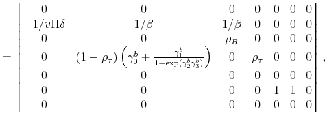
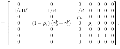
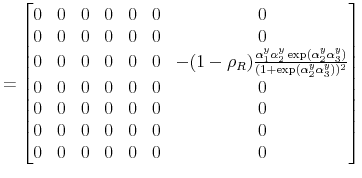
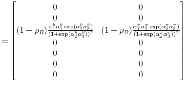
Substitute (36)-(37) in (33)-(35) to obtain
where
Then, solving for
![]() and
and
![]() , we have
, we have
Let
Then, using the relevant elements of
Given ![]() ,
, ![]() and
and ![]() ,
,
![]() takes the following expressions that include
takes the following expressions that include ![]() ,
,
![]() ,
, ![]() and
and ![]() :
:
-

-

-

-
 ,
,
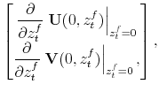
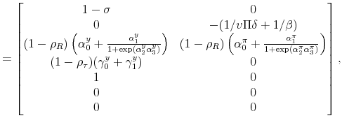
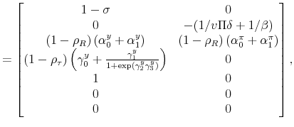
Then, to find
![]() and
and ![]() we solve the following system of equations for
the relevant elements of
we solve the following system of equations for
the relevant elements of
![]() and
and
![]() :
:

|
||

|

|
|||

|
|||
 |
|||

|
|||

|
|||
 |
where

|
||

|
||
|
||
|
||
|
||
|
 |
|
|
 |
|
|
 |
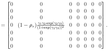
|
C..3 Finding 
Given
![]() and
and ![]() , we have the following expression
that includes
, we have the following expression
that includes ![]() :
:
 |
Then, to find
 |
D. Computation of
 and
and

To obtain
![]() and
and
![]() we perform a second order Taylor expansion to
we perform a second order Taylor expansion to
around
where
Then, taking expectation conditional to ![]() and
and ![]() , we get
, we get
Notice that the expectation of the coefficient matrices involves ![]() , the correlation coefficient between the latent factors that drive the evolution of the monetary and fiscal policy
rule coefficients. When taking expectations, the agents of the model incorporate the degree of interdependence in policymaking.
, the correlation coefficient between the latent factors that drive the evolution of the monetary and fiscal policy
rule coefficients. When taking expectations, the agents of the model incorporate the degree of interdependence in policymaking.
E. Verifying the Guessed Functional Form
Having obtained the coefficients of the logistic functions that characterize the solution, it is necessary to verify that the guessed functional forms for
![]() and
and
![]() are indeed logistic. Recall the system of equations in (60):
are indeed logistic. Recall the system of equations in (60):
 |
Notice that if both ![]() and
and ![]() were white noise processes, then both
were white noise processes, then both
![]() and
and
![]() would be constant matrices. In that case, if the coefficients on the output gap of both policy rules were constant,
would be constant matrices. In that case, if the coefficients on the output gap of both policy rules were constant,
![]() in (57) would be a function of
in (57) would be a function of ![]() only
through
only
through
![]() ,
,
![]() in (58) would be a function of
in (58) would be a function of ![]() only
through
only
through
![]() , and
, and
![]() would be constant. This implies that some of the elements of
would be constant. This implies that some of the elements of
![]() are bivariate logistic functions, and that all the elements of
are bivariate logistic functions, and that all the elements of
![]() are univariate logistic functions that depend on
are univariate logistic functions that depend on ![]() . In
particular, only the entries in the second column of
. In
particular, only the entries in the second column of
![]() , those that relate the behavior of inflation and the output gap with the evolution of lagged debt, depend on both
, those that relate the behavior of inflation and the output gap with the evolution of lagged debt, depend on both ![]() and
and ![]() ; all the other elements are univariate logistic functions dependent on
; all the other elements are univariate logistic functions dependent on ![]() . Hence, in the absence of persistence in the latent factors, it is easy to show that the solution matrices follow indeed bivariate (or univariate) logistic functions. It can be shown that the same argument holds if the policy rule
coefficients on the output gap are time varying.
. Hence, in the absence of persistence in the latent factors, it is easy to show that the solution matrices follow indeed bivariate (or univariate) logistic functions. It can be shown that the same argument holds if the policy rule
coefficients on the output gap are time varying.
In any case, however, and in particular when the latent factors are persistent, the solution has to be such that in (60) we do not `divide by zero'. The issue has to do with the fact that since the transition between states is continuous, as opposed to the Markov-switching
setup of policy rule coefficients, for some values of
![]() there may exist a discontinuity in the solution. To see this, consider the simple Fisherian model:
there may exist a discontinuity in the solution. To see this, consider the simple Fisherian model:
where the notation is the same as in the new Keynesian model, since this is a particular version of the model presented in the paper.
We guess that the fundamental solution is given by
where
Solving for ![]() , we have
, we have
 |
Performing a first-order Taylor expansion to
![]() around
around
![]() , we get
, we get
If ![]() , it is easy to see that
, it is easy to see that
 |
Hence, for the solution to be logistic --and continuous, we need
![]()
![]() , which is the same as
, which is the same as
![]() , given the monotonicity of
, given the monotonicity of
![]() .
.
To derive the analogous condition in the more general case of the model presented in the paper, rewrite (60) for
![]() ignoring the last two terms of (59), as follows:
ignoring the last two terms of (59), as follows:
which can be rewritten as
Hence, a sufficient condition for the continuity of the solution is that each of the elements of
![]() is greater than the corresponding element of
is greater than the corresponding element of
![]() .
.
F. Endogeneity Setup
Let
![]() be the demeaned government spending to output ratio in period
be the demeaned government spending to output ratio in period ![]() ,
,
![]() the annual rate of growth of M2 in period
the annual rate of growth of M2 in period ![]() , and
, and
![]() commodity price inflation. In order to account for the existence of endogeneity, the observation equations (39)-(40) of the state-space
model have to be modified by introducing a system of simultaneous equations. To that end, let
commodity price inflation. In order to account for the existence of endogeneity, the observation equations (39)-(40) of the state-space
model have to be modified by introducing a system of simultaneous equations. To that end, let
Hence, conditional on
![]() , the state-space model (39)-(44) can be divided into two models: one for the interest rate equation, and another for the tax rate
equation. The observation equations of each of the models are:
, the state-space model (39)-(44) can be divided into two models: one for the interest rate equation, and another for the tax rate
equation. The observation equations of each of the models are:
and
Here,
where
Let
![]() and
and
![]() . Appendix G shows how to obtain the conditional likelihood function of
. Appendix G shows how to obtain the conditional likelihood function of
![]() .
.
G. The Likelihood Function of the Model with Endogeneity, Time-Varying Coefficients and Stochastic Volatility
Notice that the joint density function of ![]() and
and
![]() , conditional on
, conditional on ![]() , for
, for ![]() , and the latent factors and stochastic volatility (these last two omitted from the density functions below) can be written as
, and the latent factors and stochastic volatility (these last two omitted from the density functions below) can be written as
where
Let
 |
||
 |
where
 |
is the maximum likelihood estimator of
This is the two-stage conditional maximum likelihood estimation procedure suggested by Vuong (1984). Let
![]() , and let
, and let
![]() be defined in a similar way. Let
be defined in a similar way. Let
![]() and
and
![]() . The log-likelihood function of
. The log-likelihood function of
![]() given
given
![]() is
is
 |
where
and
H. Bayesian Estimation
The method presented here extends the estimation method implemented in Geweke and Tanizaki (2001) by allowing endogeneity. Let
![]() denote the conditional density of
denote the conditional density of
![]() given
given
![]() ,
,
![]() ,
,
![]() ,
,
![]() and
and ![]() . Let
. Let
![]() denote the conditional density of
denote the conditional density of
![]() given
given
![]() and
and ![]() . Let
. Let
![]() denote the conditional density of
denote the conditional density of
![]() given
given
![]() and
and ![]() . Define
. Define
![]() and
and
![]() . Under this setup, the joint density of
. Under this setup, the joint density of
![]() ,
,
![]() and
and
![]() given
given
![]() ,
,
![]() ,
, ![]() ,
, ![]() and
and ![]() is given by
is given by
where the last equality follows from the Markov property of
 |
||
 |
||
 |
where
From the posterior densities (67)-(69), the smoothing random draws are generated as follows:
- extbfStep 1.
- Take appropriate initial values for
 ,
,  ,
,
 ,
,  and
and
 , and fix
 ,
,
 for i=1,2.12
 - extbfStep 2.
- Generate a random draw of
 from
from
 for
for
 . Draw
 using the normal proposal density

where is the filtered variance-covariance matrix of the random coefficients of a random-coefficient specification of the policy rules, and
  is a proper scale coefficient. The algorithm accepts
 with probability
  :
:

- extbfStep 3.
- Generate a random draw of
 from
from
 .
.
- Partition
 , where
 ,
,
 ,
,
 and
and
 . Partition
 , where
 ,
,
 and
and
 .
. - Generate a random draw of
 sequentially, as follows:
- Generate a random draw of a transformation of
 ,
,
 , using the normal proposal density

where is the variance-covariance matrix of the maximum likelihood estimator of
 given the initial latent factors and stochastic volatilities, and
  is a scale coefficient. The algorithm accepts
 with probability
  :
:

- Generate a random draw of a transformation of
 ,
,
 , using the normal proposal density

where is the variance-covariance matrix of the maximum likelihood estimator of
 given the initial latent factors and stochastic volatilities, and
  is a scale coefficient. The algorithm accepts
 with probability
  :
:

- Generate a random draw of
 using the normal proposal density

where is the least squares estimator of
 using the residuals of least squares estimations of (61) and (62), and
  is its least squares estimated variance-convariance matrix. The algorithm accepts
 with probability
  :
:

where is the proposal density.
- Generate a random draw of a transformation of
- Generate a random draw of
 sequentially, as follows:
- Generate a random draw of a transformation of
 ,
,
 , using the normal proposal density

where is the variance-covariance matrix of the maximum likelihood estimator of
 given the initial latent factors and stochastic volatilities, and
  is a scale coefficient. The algorithm accepts
 with probability
  :
:

- Generate a random draw of a transformation of
 ,
,
 , using the normal proposal density

where is the variance-covariance matrix of the maximum likelihood estimator of
 given the initial latent factors and stochastic volatilities, and
  is a scale coefficient. The algorithm accepts
 with probability
  :
:

- Generate a random draw of
 using the normal proposal density

where is the least squares estimator of
 using the residuals of least squares estimations of (63) and (64), and
  is its least squares estimated variance-convariance matrix. The algorithm accepts
 with probability
  :
:

where is the proposal density.
- Generate a random draw of a transformation of
- Partition
- extbfStep 4.
- Generate a random draw of
 from
from
 for
for
 . Draw
 using the normal proposal density

where is the filtered variance-covariance matrix of the volatility of a constant-coefficient specification of the policy rules, and
  is a proper scale coefficient. The algorithm accepts
 with probability
  :
:

- extbfStep 5.
- Generate a random draw of
 from
from
 sequentially, as follows:
- Partition
 where
where
 and
and
 .
. - Generate a random draw
 using two independent Beta proposal densities (expressed in terms of means and standard deviations)

 Beta
Beta

 Beta
Beta
where is the ordinary least squares estimate of
 in (41) using
 , and
, and
 is its standard error. The same applies for
 and
and
 , which come from the estimation of (42) using
 . The algorithm accepts
 with probability
  :
:

- Generate a random draw
 using a four-parameter Beta proposal density with range on [-1,1] (expressed in terms of mean and standard deviation)
 TransformedBeta
where is the correlation coefficient between the residuals of equations (41) and (42) using
 and
and
 as estimated coefficients where corresponds. The algorithm accepts
 with probability
  :
:

- Partition
- extbfStep 6.
- Generate a random draw of
 from
from
 .
.
- Partition
 where
where
 and
and
 .
. - Generate a random draw
 using the independent proposal densities (expressed in terms of means and standard deviations)

 Beta
Beta

 Beta
Beta


with and
and
 , where
 are the least squares estimates of
 and
and
 in (43), respectively, using
 , and where
 are obtained similarly from (44) using
 . The algorithm accepts
 with probability
  :
:

- Generate a random draw
 using the inverted gamma proposal densities

 IG
IG df
df

 IG
IG df
df
where and
and
 are residuals, and
 and
and
 are vectors that stack the respective residuals. The algorithm accepts
 with probability
  :
:

- Partition
- extbfStep 7.
- Repeat steps 1-4
 times to obtain
  random draws of
 ,
,
 ,
,  ,
,  and
and  .
.
In steps (ii)-(vi) the random draws of
![]() ,
,
![]() ,
, ![]() ,
, ![]() and
and ![]() are updated. This sampling method is referred to as the Gibbs sampler. To generate the random draws of
are updated. This sampling method is referred to as the Gibbs sampler. To generate the random draws of
![]() ,
,
![]() for
for
![]() ,
, ![]() ,
, ![]() and
and ![]() , we use the Metropolis-Hastings (M-H) algorithm. That is, the Gibbs sampler and the M-H algorithm are
combined to obtain the smoothing random draws from the state-space model.
, we use the Metropolis-Hastings (M-H) algorithm. That is, the Gibbs sampler and the M-H algorithm are
combined to obtain the smoothing random draws from the state-space model.
References
Ali, Mir M., N. N. Mikhail, and M. Safiul Haq (1978) `A class of bivariate distributions including the bivariate logistic.'Journal of Multivariate Analysis 8(3), 405-412
An, Sungbae, and Frank Schorfheide (2007) `Bayesian analysis of dsge models.' Econometric Reviews 26(2-4), 113-172
Bae, Jinho, Chang-Jin Kim, and Dong Heon Kim (2011) `The evolution of the monetary policy regimes in the u.s.' Discussion Paper Series 1102, Institute of Economic Research, Korea University
Bianchi, Francesco (2010) `Regime switches, agents beliefs, and post-world war ii u.s. macroeconomic dynamics.' MPRA Paper, University Library of Munich, Germany
Bianchi, Francesco (2012) `Evolving monetary fiscal policy mix in the united states.' American Economic Review 102(3), 167-72
Boivin, Jean (2006) `Has u.s. monetary policy changed? evidence from drifting coefficients and real-time data.' Journal of Money, Credit and Banking 38(5), 1149-1173
Canzoneri, Matthew, Robert E. Cumby, and Behzad T. Diba (2010) `The interaction between monetary and fiscal policy.' In Handbook of Monetary Economics,ed. Benjamin M. Friedman and Michael Woodford, 1 ed., vol. 3 (Elsevier) chapter 17, pp. 935-999
Carlstrom, Charles, and Timothy S. Fuerst (2000) `The scal theory of the price level.' Economic Review (Q I), 22-32
Cho, Seonghoon (2013) `Characterizing markov-switching rational expectations models.' Available at SSRN 1468331
Claeys, P. (2008) `Rules, and their effects on fiscal policy in sweden.' Swedish Economic Policy Review 15(1), 7
Clarida, Richard H., Jordi Gali, and Mark Gertler (2000) `Monetary policy rules and macroeconomic stability: Evidence and some theory.' The Quarterly Journal of Economics 115(1), 147-180
Cochrane, John H. (1998) `A frictionless view of u.s. in ation.' In `NBER Macroeconomics Annual 1998, volume 13' (National Bureau of Economic Research, Inc) pp. 323-421
Cochrane, John H. (2001) `Long-term debt and optimal policy in the scal theory of the price level.' Econometrica 69(1), 69-116
Cochrane, John H. (2005) `Money as stock.' Journal of Monetary Economics 52(3), 501-52
Davig, Troy, and Eric Leeper (2006) `Fluctuating macro policies and the scal theory.' In `NBER Macroeconomics Annual 2006, Volume 21' (National Bureau of Economic Research, Inc) pp. 247-316
Davig, Troy, and Eric Leeper(2007) `Generalizing the taylor principle.' American Economic Review 97(3), 607-635
Davig, Troy, and Eric Leeper (2011) `Monetary-fiscal policy interactions and fiscal stimulus.' European Economic Review 55(2), 211-227
Davig, Troy, and Taeyoung Doh (2009) `Monetary policy regime shifts and in ation persistence.' Research Working Paper RWP 08-16, Federal Reserve Bank of Kansas City
Eo, Yunjong (2009) `Bayesian analysis of dsge models with regime switching.' MPRA Paper, University Library of Munich, Germany
Farmer, Roger E. A., Daniel F. Waggoner, and Tao Zha (2008) `Minimal state variable solutions to markov-switching rational expectations models.' Working Paper 2008-23, Federal Reserve Bank of Atlanta
Eo, Yunjong (2011)`Minimal state variable solutions to markov-switching rational expectations models.' Journal of Economic Dynamics and Control 35(12), 2150-2166
Favero, Carlo, and Tommaso Monacelli (2003) `Monetary-fiscal mix and in ation performance: Evidence from the u.s.' Working Papers 234, IGIER (Innocenzo Gasparini Institute for Economic Research), Bocconi University
Fernandez-Villaverde, Jesus, Pablo A. Guerron, and Juan F Rubio-Ramirez (2010) `Fortune or virtue: Time-variant volatilities versus parameter drifting in u.s. data.' NBER Working Papers 15928, National Bureau of Economic Research, Inc
Fernandez-Villaverde, Jesus, Pablo A. Guerron, Juan F Rubio-Ramirez, and Martin Uribe (2011a) `Risk matters: The real effects of volatility shocks.' American Economic Review 101(6), 2530-61
Fernandez-Villaverde, Jesus, Pablo A. Guerron, Keith Kuester, and Juan F Rubio-Ramirez (2011b) `Fiscal volatility shocks and economic activity.' NBER Working Papers 17317, National Bureau of Economic Research, Inc
Foerster, Andrew, Juan F. Rubio-Ramirez, Daniel F. Waggoner, and Tao Zha (2013) `Perturbation methods for markov-switching models.' Research Working Papers RWP 13-01, The Federal Reserve Bank of Kansas City
Friedman, Milton (1948) `A monetary and fiscal framework for economic stability.' The American Economic Review 38(3), pp. 245-264
Geweke, John, and Hisashi Tanizaki (2001) `Bayesian estimation of state-space models using the metropolis-hastings algorithm within gibbs sampling.' Computational Statistics and Data Analysis 37(2), 151-170
Hetzel, Robert L. (2008) The Monetary Policy of the Federal Reserve: A History (Studies in Macroeconomic History),1 ed. (Cambridge University Press)
Keen, Benjamin David, and Yongsheng Wang (2007) `What is a realistic value for price adjustment costs in new keynesian models?' Applied Economics Letters 14(11), 789-793
Kim, Chang-Jin (2006) `Time-varying parameter models with endogenous regressors.' Economics Letters 91(1), 21-26
Kim, Chang-Jin (2009) `Markov-switching models with endogenous explanatory variables ii: A two-step mle procedure.' Journal of Econometrics 148(1), 46-55
Kim, Chang-Jin, and Charles R. Nelson (2006a) `Estimation of a forward-looking monetary policy rule: A time-varying parameter model using ex post data.' Journal of Monetary Economics 53(8), 1949-1966
Kim, Chang-Jin, and Charles R. Nelson (2006b) `Estimation of a forward-looking monetary policy rule: A time-varying parameter model using ex post data.' Journal of Monetary Economics 53(8), 1949-1966
Kim, Soyoung (2003) `Structural shocks and the fiscal theory of the price level in the sticky price model.' Macroeconomic Dynamics 7(05), 759-782
Leeper, Eric (1991) `Equilibria under 'active' and 'passive' monetary and scal policies.' Journal of Monetary Economics 27(1), 129-147
Leith, Campbell, and Simon Wren-Lewis (2000) `Interactions between monetary and fiscal policy rules.' Economic Journal 110(462), C93-108
Li, Bing (2009) `On the identification of fiscal policy behavior.' Technical Report, CAEPR Working Paper
Lubik, Thomas, and Frank Schorfheide (2004) `Testing for indeterminacy: An Application to US Monetary Policy.' The American Economic Review 94(1), 190-217
McCallum, Bennett (1983) `On non-uniqueness in rational expectations models: An attempt at perspective.' Journal of Monetary Economics 11(2), 139-168
Raftery, Adrian E., and Steven Lewis (1992) `How many iterations in the gibbs sampler?' In `In Bayesian Statistics 4' Oxford University Press pp. 763-773
Sargent, T.J., and N. Wallace (1981) `Some unpleasant monetarist arithmetic.' Federal Reserve Bank of Minneapolis Quarterly Review 5(3), 1-17
Sims, Christopher (1992) `Interpreting the macroeconomic time series facts: The effects of monetary policy.' European Economic Review 36(5), 975-1000
Sims, Christopher (1994) `A simple model for study of the determination of the price level and the interaction of monetary and fiscal policy.' Economic Theory 4(3), 381-99
Sims, Christopher (2011) `Stepping on a rake: The role of fiscal policy in the in ation of the 1970s.' European Economic Review 55(1), 48-56. Special Issue on Monetary and Fiscal Interactions in Times of Economic Stress
Sims, Christopher, and Tao Zha (2006) `Were there regime switches in u.s. monetary policy?' American Economic Review 96(1), 54-81
Stock, James H., and Mark W. Watson (2002) `Has the business cycle changed and why?' Working Paper 9127, National Bureau of Economic Research, August
Taylor, John B. (1993) `Discretion versus policy rules in practice.' Carnegie-Rochester Conference Series on Public Policy 39(1), 195-214
Uhlig, Harald (1998) `A toolkit for analysing nonlinear dynamic stochastic models easily.' QM&RBC Codes, Quantitative Macroeconomics & Real Business Cycles
Vuong, Quang H. (1984) `Two-stage conditional maximum likelihood estimation of econometric models.' Working Papers 538, California Institute of Technology, Division of the Humanities and Social Sciences, July
Woodford, Michael (1994) `Monetary policy and price level determinacy in a cash-in-advance economy.' Economic Theory 4, 345-380
Woodford, Michael (1995) `Price-level determinacy without control of a monetary aggregate.' Carnegie Rochester Conference Series on Public Policy 43(0), 1-46
Woodford, Michael (1996) `Control of the public debt: A requirement for price stability?' NBER Working Papers 5684, National Bureau of Economic Research, Inc
Yksel, Ebru, Kivilcim Metin-Ozcan, and Ozan Hatipoglu (2013) `A survey on time-varying parameter taylor rule: A model modified with interest rate pass-through.' Economic Systems 37(1), 122-134
Footnotes
 and
and
 , where
  |
where
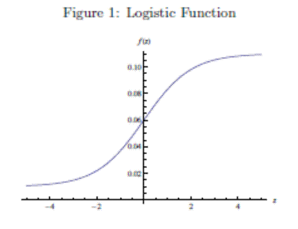


 MRS
MRS![\displaystyle _{0,t} \left[\frac{P_t(j)}{P_t}Y_t(j) - \frac{W_t}{P_t}L_t(j) - \frac{\phi}{2}\left( \frac{P_t(j)}{\Pi P_{t-1}(j) }-1 \right)^2 Y_t\right],](img136.gif)


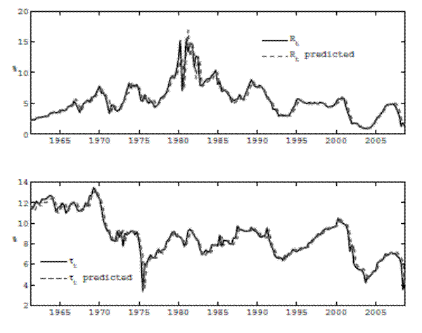
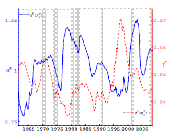
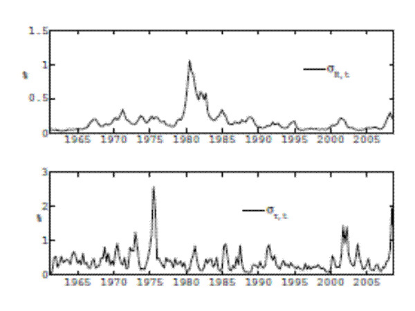
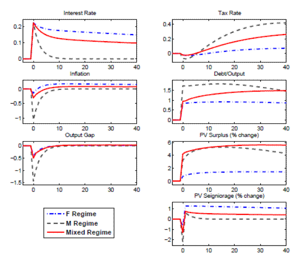
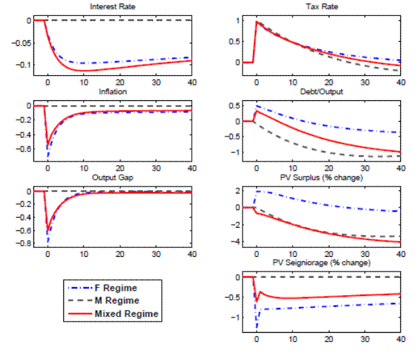
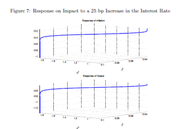
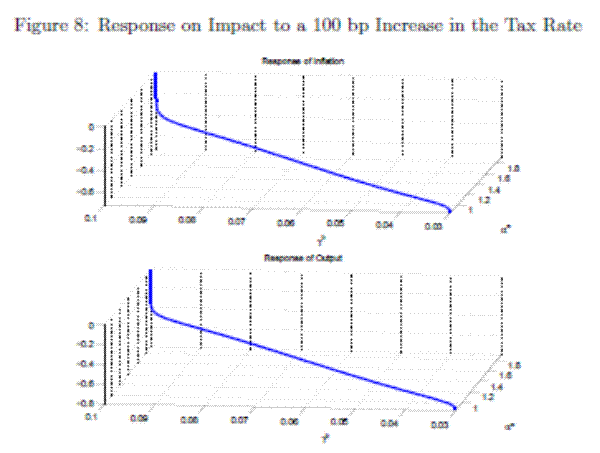
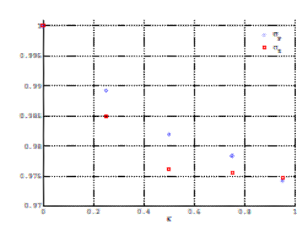


![\displaystyle \lambda_t Y_t \left[ (1-\theta_t)\left(\frac{P_t(j)}{P_t}\right)^{-\theta_t}\frac{1}{P_t} + \theta_t \frac{\psi_t}{P_t} \left(\frac{P_t(j)}{P_t}\right)^{-\theta_t-1} - \phi\left(\frac{P_t(j)}{\Pi P_{t-1}}-1\right) \frac{1}{\Pi P_{t-1}(j)}\right] + \notag](img338.gif)

![\displaystyle \frac{D_t(j)}{P_t} = \frac{D_t}{P_t} = \left[ 1 - \psi_t - \frac{\phi}{2}\left( \frac{P_t}{\Pi P_{t-1} }-1 \right)^2\right]Y_t.](img343.gif)


