
Board of Governors of the Federal Reserve System
International Finance Discussion Papers
Number 990, January 2010 --- Screen Reader
Version*
Firm-Specific Capital, Nominal Rigidities and the Business Cycle1
NOTE: International Finance Discussion Papers are preliminary materials circulated to stimulate discussion and critical comment. References in publications to International Finance Discussion Papers (other than an acknowledgment that the writer has had access to unpublished material) should be cleared with the author or authors. Recent IFDPs are available on the Web at http://www.federalreserve.gov/pubs/ifdp/. This paper can be downloaded without charge from the Social Science Research Network electronic library at http://www.ssrn.com/.
Abstract:
This paper formulates and estimates a three-shock US business cycle model. The estimated model accounts for a substantial fraction of the cyclical variation in output and is consistent with the observed inertia in inflation. This is true even though firms in the model reoptimize prices on average once every 1.8 quarters. The key feature of our model underlying this result is that capital is firm-specific. If we adopt the standard assumption that capital is homogeneous and traded in economy-wide rental markets, we find that firms reoptimize their prices on average once every 9 quarters. We argue that the micro implications of the model strongly favor the firm-specific capital specification.
JEL classification: E3, E4, E5
1. Introduction
Macroeconomic data indicate that inflation is inertial. To account for this inertia, macro modeler embed assumptions that are either implausibe on a priori grounds or directly in conflict with micro data. For example, in many new-Keynesian macroeconomic models, firms index non-optimized prices to lagged inflation. These models account for inflation inertia by assuming that firms re-optimize their prices every six quarters or even less often.6 Other new-Keynesian models don't allow for indexing to lagged inflation. In estimated versions of these models, firms change prices once every two years or less often.7 This property contrasts sharply with findings in Bils and Klenow (2004), Golosov and Lucas (2007) and Klenow and Kryvstov (2008) who argue that firms change prices more frequently than once every two quarters.8
In this paper we formulate and estimate a model which is consistent with the evidence of inertia in inflation, even though firms re-optimize prices on average once every 1.8 quarters.9 In addition our model accounts for the dynamic response of 10 key U.S. macro time series to monetary policy shocks, neutral technology shocks and capital embodied shocks.10
In our model aggregate inflation is inertial despite the fact that firms re-optimize prices frequently. The inertia reflects that when firms do re-optimize prices, they change prices by a small amount. Firms change prices by a small amount because each firm's short run marginal cost curve is increasing in its own output.11 This positive dependency reflects our assumption that in any given period, a firm's capital stock is pre-determined. In standard equilibrium business cycle models a firm's capital stock is not pre-determined and all factors of production, including capital, can be instantly and costlessly transferred across firms. These assumptions are empirically unrealistic but are defended on the grounds of tractability. The hope is that these assumption are innocuous and do not affect major model properties. In fact these assumptions matter a lot.
In our model, a firm's capital is pre-determined and can only be changed over time by varying the rate of investment. These properties follow from our assumption that capital is completely firm-specific. Our assumptions about capital imply that a firm's marginal cost curve depends positively on its output level.12 To see the impact of this dependence on pricing decisions, consider a firm that contemplates raising its price. The firm understands that a higher price implies less demand and less output. A lower level of output reduces marginal cost, which other things equal, induces a firm to post a lower price. Thus, the dependence of marginal cost on firm-level output acts as a countervailing influence on a firm's incentives to raise price. This countervailing influence is why aggregate inflation responds less to a given aggregate marginal cost shock when capital is firm-specific.
Anything, including firm-specificity of some other factor of production or adjustment costs in labor, which causes a firm's marginal cost to be an increasing function of its output works in the same direction as firm-specificity of capital. This fact is important because our assumption that the firm's entire stock of capital is predetermined probably goes too far from an empirical standpoint.
We conduct our analysis using two versions of the model analyzed
by Christiano, Eichenbaum, and Evans (CEE henceforth, 2005): in
one, capital is homogeneous whereas in the other, it is firm
specific. We refer to these models as the homogeneous and
firm-specific capital models, respectively. We show that the only
difference between the log-linearized equations characterizing
equilibrium in the two models pertains to the equation relating
inflation to marginal costs. The form of this equation is identical
in both models: the change in inflation at time ![]() is
equal to discounted expected change in inflation at time
is
equal to discounted expected change in inflation at time
![]() plus a reduced form coefficient,
plus a reduced form coefficient,
![]() , multiplying time
, multiplying time ![]() economy-wide average real marginal cost. The difference between the
two models lies in the mapping between the structural parameters
and
economy-wide average real marginal cost. The difference between the
two models lies in the mapping between the structural parameters
and ![]() . In non-linear framework, however, it
is not true that the solutions to the homogeneous and firm-specific
capital models are obserbationally equivalent with respect to macro
data.13
. In non-linear framework, however, it
is not true that the solutions to the homogeneous and firm-specific
capital models are obserbationally equivalent with respect to macro
data.13
In the homogeneous capital model, ![]() depends
only on agents' discount rates and on the fraction,
depends
only on agents' discount rates and on the fraction, ![]() , of firms that re-optimize prices within the
quarter. In the firm-specific capital model,
, of firms that re-optimize prices within the
quarter. In the firm-specific capital model, ![]() is a function of a broader set of the structural
parameters. For example, the more costly it is for a firm to vary
capital utilization, the steeper is its marginal cost curve and
hence the smaller is
is a function of a broader set of the structural
parameters. For example, the more costly it is for a firm to vary
capital utilization, the steeper is its marginal cost curve and
hence the smaller is ![]() . A different example is
that in the firm-specific capital model, the parameter
. A different example is
that in the firm-specific capital model, the parameter ![]() is smaller the more elastic is the firm's demand
curve.14 This result reflects that the more
elastic is a firm's demand, the greater is the reduction in demand
and output in response to a given price increase. A bigger fall in
output implies a bigger fall in marginal cost which reduces a
firm's incentive to raise its price.
is smaller the more elastic is the firm's demand
curve.14 This result reflects that the more
elastic is a firm's demand, the greater is the reduction in demand
and output in response to a given price increase. A bigger fall in
output implies a bigger fall in marginal cost which reduces a
firm's incentive to raise its price.
The only way that ![]() enters into the
reduced form of the two models is via its impact on
enters into the
reduced form of the two models is via its impact on ![]() . If we parameterize the two models in terms of
. If we parameterize the two models in terms of
![]() rather than
rather than ![]() ,
they have identical implications for all aggregate quantities and
prices in a standard (log-)linearized framework. This observational
equivalence result implies that we can estimate the model in terms
of
,
they have identical implications for all aggregate quantities and
prices in a standard (log-)linearized framework. This observational
equivalence result implies that we can estimate the model in terms
of ![]() without taking a stand on whether
capital is firm-specific or homogeneous. The observational
equivalence result also implies that we cannot assess the relative
plausibility of the homogeneous and firm-specific capital models
using macro data. However, the two models have very different
implications for micro data. To assess the relative plausibility of
the two models, we focus on the mean time between price
re-optimization, and the dynamic response of the cross - firm
distribution of production and prices to aggregate shocks. These
implications depend on the parameters of the model, which we
estimate.
without taking a stand on whether
capital is firm-specific or homogeneous. The observational
equivalence result also implies that we cannot assess the relative
plausibility of the homogeneous and firm-specific capital models
using macro data. However, the two models have very different
implications for micro data. To assess the relative plausibility of
the two models, we focus on the mean time between price
re-optimization, and the dynamic response of the cross - firm
distribution of production and prices to aggregate shocks. These
implications depend on the parameters of the model, which we
estimate.
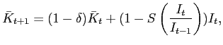
We follow CEE (2005) in choosing model parameter values to minimize the differences between the dynamic response to shocks in the model and the analog objects estimated using a vector autoregressive representation of 10 post-war quarterly U.S. time series.15 To compute vector autoregression (VAR) based impulse response functions, we use identification assumptions satisfied by our economic model: the only shocks that affect productivity in the long run are innovations to neutral and capital-embodied technology; the only shock that affects the price of investment goods in the long run is an innovation to capital-embodied technology;16 monetary policy shocks have a contemporaneous impact on the interest rate, but they do not have a contemporaneous impact on aggregate quantities or the price of investment goods. We estimate that together these three shocks account for almost 60 percent of cyclical fluctuations in aggregate output and other aggregate quantities.
We now discuss the key properties of our estimated model. First,
the model does a good job of accounting for the estimated response
of the economy to both monetary policy and technology shocks.
Second, according to our point estimates, households re-optimize
wages on average about once a year. Third, our point estimate of
![]() is 0.014. In the
homogeneous capital version of the model, this value of
is 0.014. In the
homogeneous capital version of the model, this value of ![]() implies that firms change prices on average once every
9.4 quarters. But in the firm-specific
capital model, this value of
implies that firms change prices on average once every
9.4 quarters. But in the firm-specific
capital model, this value of ![]() implies that
firms change price on average once every 1.8
quarters. The reason why the models have such different
implications for firms' pricing behavior is that according to our
estimates, firms' demand curves are highly elastic and their
marginal cost curves are very steep.
implies that
firms change price on average once every 1.8
quarters. The reason why the models have such different
implications for firms' pricing behavior is that according to our
estimates, firms' demand curves are highly elastic and their
marginal cost curves are very steep.
Finally, we show that the two versions of the model differ sharply in terms of their implications for the cross-sectional distribution of production. In the homogeneous capital model, a very small fraction of firms produce the bulk of the economy's output in the periods after a monetary policy shock. The implications of the firm-specific model are much less extreme. We conclude that both the homogeneous and firm-specific capital models can account for inflation inertia and the response of the economy to monetary policy and technology shocks. But only the firm-specific model can reconcile the micro-macro pricing conflict without obviously unpalatable micro implications.
It is useful to place this paper in the context of the
literature. That firm-specific capital can rationalize a lower
estimate of ![]() (more frequent price
re-optimization) was first demonstrated by Sbordone (1998, 2002)
and further discussed by Gali, Gertler and Lopez-Salido (2001) and
Woodford (2003). In these papers, the stock of capital owned by the
firm is fixed. Woodford (2005) analyzes the impact of firm specific
capital allowing for investment. As our discussion above indicates,
whether firm specific capital actually does rationalize a lower
estimate of
(more frequent price
re-optimization) was first demonstrated by Sbordone (1998, 2002)
and further discussed by Gali, Gertler and Lopez-Salido (2001) and
Woodford (2003). In these papers, the stock of capital owned by the
firm is fixed. Woodford (2005) analyzes the impact of firm specific
capital allowing for investment. As our discussion above indicates,
whether firm specific capital actually does rationalize a lower
estimate of ![]() depends critically on the other
parameters characterizing firms' environments. To the extent that
capital utilization rates can easily be varied, the assumption of
firm specific capital loses its ability to rationalize low values
of
depends critically on the other
parameters characterizing firms' environments. To the extent that
capital utilization rates can easily be varied, the assumption of
firm specific capital loses its ability to rationalize low values
of ![]() A maintained assumption of the
papers just cited is that firms cannot vary capital utilization
rates. So these papers leave open the question of how important
firm specific capital is once firms can vary capital utilization
rates. Similarly, the smaller is the elasticity of demand for a
firm's output, the smaller is the impact of firm specific capital
on inference about
A maintained assumption of the
papers just cited is that firms cannot vary capital utilization
rates. So these papers leave open the question of how important
firm specific capital is once firms can vary capital utilization
rates. Similarly, the smaller is the elasticity of demand for a
firm's output, the smaller is the impact of firm specific capital
on inference about ![]() The above cited
papers condition their inference on particular assumed values for
this elasticity. The key contribution of this paper is to estimate
the key parameters governing the operational importance of firm
specific capital and to assess the importance for firm specific
capital in an estimated dynamic stochastic general equilibrium
model. Our key result is that the assumption of firm specific
capital does in fact rationalize relatively low values of
The above cited
papers condition their inference on particular assumed values for
this elasticity. The key contribution of this paper is to estimate
the key parameters governing the operational importance of firm
specific capital and to assess the importance for firm specific
capital in an estimated dynamic stochastic general equilibrium
model. Our key result is that the assumption of firm specific
capital does in fact rationalize relatively low values of
![]() thereby helping to reconcile the
apparent conflicting pictures of pricing behavior painted by micro
and macro data.17
thereby helping to reconcile the
apparent conflicting pictures of pricing behavior painted by micro
and macro data.17
From a broader perspective, this paper belongs to a larger literature that tries to explain the mechanisms by which nominal shocks have effects on real economic activity that last longer than the frequency with which firms re-optimize prices. Perhaps the most closely related mechanisms are firm specific labor (Woodford (2005)), sector specific labor (Gertler and Leahy (2008)) and strategic complementarities arising from an elasticity of firm demand that is increasing in the firm's price (see for example Kimble (1995) and Eichenbaum and Fisher (2007)). A different propagation mechanism stems from heterogeneity across sectors in the frequency of price changes (see for example Bils and Klenow (2004), Carvalho (2006) and Steinsson and Nakamura (2008)) and the presence of intermediate inputs (see for example Basu (1995) and Huang (2006)).
An alternative and promising propagation mechanism arises from the assumption that firms cannot attend perfectly to all available information (see Sims (1998, 2003)). Mackowiak and Wiederholdt (2008) present a model in which firms decide what variables to pay attention to, subject to a constraint on information flow. When idiosyncratic conditions are more variable or more important than aggregate conditions, firms in their model pay more attention to idiosyncratic conditions than to aggregate conditions. Their model has the important property that firms react fast and by large amounts to idiosyncratic shocks, but only slowly and by small amounts to nominal shocks. As a result nominal shocks have strong and persistent real effects. Woodford (2008) develops a generalization of the standard, full-information model of state-dependent pricing in which decisions about when to review a firm's existing price must be made on the basis of imprecise awareness of current market conditions. He endogenizes imperfect information using a variant of the theory of " rational inattention" proposed by Sims (1998, 2003)). In related work, Mankiw and Reis (2002) and Reis (2006) stress the potential importance of slow dissemination of information to firms for generating persistent effects of nominal shocks.
The merits of these alternative propagation mechansims is a subject of an ongoing, vigorous debate. A detailed assessment of their empirical strengths is beyond the scope of this paper. It is clear however that the debate will be settled on the field of microeconomic data. For recent reviews of how firm level data on prices bears on alternative approaches we refer the reader to Mackowiak and Smets (2008), Eichenbaum, Jaimovich and Rebelo (2009), and Klenow and Malin (2009). While we emphasize the importance of firm specific capital in this paper, we leave open the possibility that the other propagation mechanisms discussed above may be at least as important.
The remainder of this paper is organized as follows. In Section 2 we describe our basic model economy. Section 3 describes our VAR-based estimation procedure. Section 4 presents our VAR-based impulse response functions and their properties. Sections 5 and 6 present and analyze the results of estimating our model. Section 7 discusses the implications of the homogeneous and firm-specific capital models for the cross-firm distribution of prices and production in the wake of a monetary policy shock. Section 8 concludes.
2. The Model Economy
In this section we describe the homogeneous and firm-specific capital models.
2.1. The Homogeneous Capital Model
The model economy is populated by goods-producing firms, households and the government.
2.1.1. Final Good Firms
At time ![]() , a final consumption good,
, a final consumption good, ![]() is produced by a perfectly competitive, representative
firm. The firm produces the final good by combining a continuum of
intermediate goods, indexed by
is produced by a perfectly competitive, representative
firm. The firm produces the final good by combining a continuum of
intermediate goods, indexed by
![]() using the technology
using the technology
![$\displaystyle Y_{t}=\left[ \int_{0}^{1}y_{t}(i)^{\frac{1}{\lambda_{f}}}di\right] ^{\lambda_{f}},$](img31.gif)
|
(1) |
where
![]() and
and ![]() denotes the time
denotes the time ![]() input of
intermediate good
input of
intermediate good ![]() The firm takes its output
price,
The firm takes its output
price, ![]() and its input prices,
and its input prices, ![]() as given and beyond its control. The first order
necessary condition for profit maximization is:
as given and beyond its control. The first order
necessary condition for profit maximization is:
|
(2) |
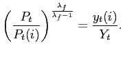
Integrating (2) and imposing (1), we obtain the following relationship between the price of the final good and the price of the intermediate good:
![$\displaystyle P_{t}=\left[ \int_{0}^{1}P_{t}(i)^{\frac{1}{1-\lambda_{f}}}di\right] ^{\left( 1-\lambda_{f}\right) }.$](img39.gif)
|
(3) |
2.1.2. Intermediate Good Firms
Intermediate good ![]() is produced by a
monopolist using the following technology:
is produced by a
monopolist using the following technology:
![$\displaystyle y_{t}(i)=\left\{ \begin{array}[c]{ll} K_{t}(i)^{\alpha}\left( z_{t}h_{t}(i)\right) ^{1-\alpha}-\phi z_{t}^{\ast} & \text{if }K_{t}(i)^{\alpha}\left( z_{t}h_{t}(i)\right) ^{1-\alpha}\geq\phi z_{t}^{\ast}\\ 0 & \text{otherwise} \end{array} \right.$](img41.gif)
|
(4) |
where
![]() Here,
Here, ![]() and
and ![]() denote time
denote time
![]() labor and capital services used to produce
the
labor and capital services used to produce
the ![]() intermediate good. The variable,
intermediate good. The variable,
![]() represents a time
represents a time ![]() shock to the technology for producing intermediate output. We refer
to
shock to the technology for producing intermediate output. We refer
to ![]() as a neutral technology shock and
denote its growth rate,
as a neutral technology shock and
denote its growth rate,
![]() by
by ![]() The
non-negative scalar,
The
non-negative scalar, ![]() parameterizes fixed
costs of production. The variable,
parameterizes fixed
costs of production. The variable,
![]() is given by:
is given by:
|
(5) |
where
![]() represents a time
represents a time ![]() shock to capital-embodied technology. We choose the
structure of the firm's fixed cost in (5) to
ensure that the non-stochastic steady state of the economy exhibits
a balanced growth path. We denote the growth rate of
shock to capital-embodied technology. We choose the
structure of the firm's fixed cost in (5) to
ensure that the non-stochastic steady state of the economy exhibits
a balanced growth path. We denote the growth rate of
![]() and
and
![]() by
by
![]() and
and
![]() respectively, so that:
respectively, so that:
| (6) |
Throughout, we rule out entry into and exit from the production of
intermediate good ![]()
Let
![]() denote
denote
![]() where
where
![]() is the growth rate of
is the growth rate of ![]() in non-stochastic steady state. We define all
variables with a hat in an analogous manner. The variables
in non-stochastic steady state. We define all
variables with a hat in an analogous manner. The variables
![]() evolves according to:
evolves according to:
| (7) |
where ![]()
![]()
![]() and
and
![]() is uncorrelated over
time and with all other shocks in the model. We denote the standard
deviation of
is uncorrelated over
time and with all other shocks in the model. We denote the standard
deviation of
![]() by
by
![]() Similarly, we assume:
Similarly, we assume:
| (8) |
where
Intermediate good firms rent capital and labor in perfectly
competitive factor markets. Profits are distributed to households
at the end of each time period. Let
![]() and
and
![]() denote the nominal rental rate on
capital services and the wage rate, respectively. We assume that
the firm must borrow the wage bill in advance at the gross interest
rate,
denote the nominal rental rate on
capital services and the wage rate, respectively. We assume that
the firm must borrow the wage bill in advance at the gross interest
rate, ![]()
Firms set prices according to a variant of the mechanism spelled
out in Calvo (1983). In each period, an intermediate goods firm
faces a constant probability,
![]() of being able to re-optimize its
nominal price. The ability to re-optimize prices is independent
across firms and time. As in CEE (2005), we assume that a firm
which cannot re-optimize its price sets
of being able to re-optimize its
nominal price. The ability to re-optimize prices is independent
across firms and time. As in CEE (2005), we assume that a firm
which cannot re-optimize its price sets ![]() according to:
according to:
| (9) |
Here, ![]() denotes aggregate inflation,
denotes aggregate inflation,
![]()
An intermediate goods firm's objective function is:
![$\displaystyle E_{t}\sum_{j=0}^{\infty}\beta^{j}\upsilon_{t+j}\left[ P_{t+j}(i)y_{t+j} (i)-P_{t+j}\left( w_{t+j}R_{t+j}h_{t+j}(i)+r_{t+j}^{k}K_{t+j}(i)\right) \right] ,$](img88.gif)
|
(10) |
where ![]() is the expectation operator conditioned
on time
is the expectation operator conditioned
on time ![]() information. The term,
information. The term,
![]() is proportional to
the state-contingent marginal value of a dollar to a
household.18 Also,
is proportional to
the state-contingent marginal value of a dollar to a
household.18 Also, ![]() is a
scalar between zero and unity. The timing of events for a firm is
as follows. At the beginning of period
is a
scalar between zero and unity. The timing of events for a firm is
as follows. At the beginning of period ![]() the firm
observes the technology shocks and sets its price,
the firm
observes the technology shocks and sets its price, ![]() . Then, a shock to monetary policy is realized, as is
the demand for the firm's product, (2). The firm
then chooses productive inputs to satisfy this demand. The problem
of the
. Then, a shock to monetary policy is realized, as is
the demand for the firm's product, (2). The firm
then chooses productive inputs to satisfy this demand. The problem
of the ![]() intermediate good firm is to choose
prices, employment and capital services, subject to the timing and
other constraints described above, to maximize (10).
intermediate good firm is to choose
prices, employment and capital services, subject to the timing and
other constraints described above, to maximize (10).
2.1.3. Households
There is a continuum of households, indexed by
![]() The sequence of events in a period
for a household is as follows. First, the technology shocks are
realized. Second, the household makes its consumption and
investment decisions, decides how many units of capital services to
supply to rental markets, and purchases securities whose payoffs
are contingent upon whether it can re-optimize its wage decision.
Third, the household sets its wage rate. Fourth, the monetary
policy shock is realized. Finally, the household allocates its
beginning of period cash between deposits at the financial
intermediary and cash to be used in consumption transactions.
The sequence of events in a period
for a household is as follows. First, the technology shocks are
realized. Second, the household makes its consumption and
investment decisions, decides how many units of capital services to
supply to rental markets, and purchases securities whose payoffs
are contingent upon whether it can re-optimize its wage decision.
Third, the household sets its wage rate. Fourth, the monetary
policy shock is realized. Finally, the household allocates its
beginning of period cash between deposits at the financial
intermediary and cash to be used in consumption transactions.
Each household is a monopoly supplier of a differentiated labor service, and sets its wage subject to Calvo-style wage frictions. In general, households earn different wage rates and work different amounts. A straightforward extension of arguments in Erceg, Henderson, and Levin (2000) and Woodford (1996) establishes that in the presence of state contingent securities, households are homogeneous with respect to consumption and asset holdings. Our notation reflects this result.
The preferences of the ![]() household are
given by:
household are
given by:
![$\displaystyle E_{t}^{j}\sum_{l=0}^{\infty}\beta^{l-t}\left[ \log\left( C_{t+l} -bC_{t+l-1}\right) -\psi_{L}\frac{h_{j,t+l}^{2}}{2}\right] ,$](img98.gif)
|
(11) |
where
![]() and
and ![]() is
the time
is
the time ![]() expectation operator, conditional on
household
expectation operator, conditional on
household ![]() 's time
's time ![]() information
set. The variable,
information
set. The variable, ![]() denotes time
denotes time
![]() consumption, and
consumption, and ![]() denotes time
denotes time ![]() hours worked. When
hours worked. When ![]() (11) exhibits habit
formation in consumption preferences.
(11) exhibits habit
formation in consumption preferences.
The household's asset evolution equation is given by:
| (12) | ||
Here, ![]()
![]() and
and
![]() denote the household's beginning of
period
denote the household's beginning of
period ![]() stock of money, cash balances and time
stock of money, cash balances and time
![]() nominal wage rate, respectively. In
addition,
nominal wage rate, respectively. In
addition,
![]()
![]() and
and ![]() denote
the household's physical stock of capital, the capital utilization
rate, firm profits and the net cash inflow from participating in
state-contingent securities at time
denote
the household's physical stock of capital, the capital utilization
rate, firm profits and the net cash inflow from participating in
state-contingent securities at time ![]() ,
respectively. The variable
,
respectively. The variable ![]() represents the
gross growth rate of the economy-wide per capita stock of money,
represents the
gross growth rate of the economy-wide per capita stock of money,
![]() The quantity
The quantity
![]() is a lump-sum payment
made to households by the monetary authority. The household
deposits
is a lump-sum payment
made to households by the monetary authority. The household
deposits
![]() with a
financial intermediary. The variable,
with a
financial intermediary. The variable, ![]() denotes
the gross interest rate.
denotes
the gross interest rate.
In (12), the price of investment goods
relative to consumption goods is given by
![]() which we assume is an
exogenous stochastic process. One way to rationalize this
assumption is that agents transform final goods into investment
goods using a linear technology with slope
which we assume is an
exogenous stochastic process. One way to rationalize this
assumption is that agents transform final goods into investment
goods using a linear technology with slope
![]() This rationalization also
underlies why we refer to
This rationalization also
underlies why we refer to
![]() as capital-embodied
technological progress.
as capital-embodied
technological progress.
The variable,
![]() denotes the time
denotes the time
![]() velocity of the household's cash
balances:
velocity of the household's cash
balances:
 |
(13) |
where
![]() is increasing and
convex. The function
is increasing and
convex. The function
![]() captures the role of
cash balances in facilitating transactions. Similar specifications
have been used by a variety of authors including Sims (1994) and
Schmitt-Grohe and Uribe (2004). For the quantitative analysis of
our model, we require the level and the first two derivatives of
the transactions function,
captures the role of
cash balances in facilitating transactions. Similar specifications
have been used by a variety of authors including Sims (1994) and
Schmitt-Grohe and Uribe (2004). For the quantitative analysis of
our model, we require the level and the first two derivatives of
the transactions function,
![]() evaluated in steady
state. We denote these by
evaluated in steady
state. We denote these by ![]()
![]() and
and
![]() respectively. We chose
values for these objects as follows. The first order condition for
respectively. We chose
values for these objects as follows. The first order condition for
![]() is:
is:
Let
![]() denote the interest
semi-elasticity of money demand:
denote the interest
semi-elasticity of money demand:
Denote the curvature of ![]() by
by ![]() :
:

Then, the first order condition for ![]() implies
that the interest semi-elasticity of money demand in steady state
is:
implies
that the interest semi-elasticity of money demand in steady state
is:
where the steady state value of ![]() is
is
![]() We parameterize
We parameterize
![]() indirectly using
values for
indirectly using
values for ![]()
![]() and
and ![]()
The remaining terms in (12) pertain to the
household's capital-related income. The services of capital,
![]() are related to stock of physical
capital,
are related to stock of physical
capital,
![]() by
by
The term
![]() represents
the household's earnings from supplying capital services. The
function
represents
the household's earnings from supplying capital services. The
function
![]() denotes the cost, in
investment goods, of setting the utilization rate to
denotes the cost, in
investment goods, of setting the utilization rate to ![]() We assume
We assume ![]() is increasing and
convex. These assumptions capture the idea that the more intensely
the stock of capital is utilized, the higher are maintenance costs
in terms of investment goods. Our log-linear approximation solution
strategy requires the level and first two derivatives of
is increasing and
convex. These assumptions capture the idea that the more intensely
the stock of capital is utilized, the higher are maintenance costs
in terms of investment goods. Our log-linear approximation solution
strategy requires the level and first two derivatives of
![]() in steady state. We
treat
in steady state. We
treat
![]() as a
parameter to be estimated and impose that
as a
parameter to be estimated and impose that ![]() and
and ![]() in steady state. Although the steady
state of the model does not depend on the value of
in steady state. Although the steady
state of the model does not depend on the value of
![]() the dynamics do. Given our
solution procedure, we do not need to specify any other features of
the function
the dynamics do. Given our
solution procedure, we do not need to specify any other features of
the function ![]()
The household's stock of physical capital evolves according to:
|
(14) |
where ![]() denotes the physical rate of
depreciation, and
denotes the physical rate of
depreciation, and ![]() denotes time
denotes time
![]() investment goods. The adjustment cost
function,
investment goods. The adjustment cost
function, ![]() is assumed to be increasing, convex
and to satisfy
is assumed to be increasing, convex
and to satisfy
![]() in steady state. We treat the
second derivative of
in steady state. We treat the
second derivative of ![]() in steady state,
in steady state,
![]() as a parameter to be
estimated. Although the steady state of the model does not depend
on the value of
as a parameter to be
estimated. Although the steady state of the model does not depend
on the value of
![]() the dynamics do. Given our
solution procedure, we do not need to specify any other features of
the function
the dynamics do. Given our
solution procedure, we do not need to specify any other features of
the function ![]()
2.1.4. The Wage Decision
As in Erceg, Henderson, and Levin (2000), we assume that the
![]() household is a monopoly supplier of a
differentiated labor service,
household is a monopoly supplier of a
differentiated labor service, ![]() . It sells
this service to a representative, competitive firm that transforms
it into an aggregate labor input,
. It sells
this service to a representative, competitive firm that transforms
it into an aggregate labor input, ![]() using
the technology:
using
the technology:
![$\displaystyle H_{t}=\left[ \int_{0}^{1}h_{j,t}^{\frac{1}{\lambda_{w}}}dj\right] ^{\lambda_{w}},$](img179.gif)
The demand curve for ![]() is given by:
is given by:
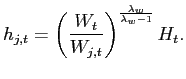
|
(15) |
Here, ![]() is the aggregate wage rate, i.e., the
nominal price of
is the aggregate wage rate, i.e., the
nominal price of ![]() It is straightforward to show
that
It is straightforward to show
that ![]() is related to
is related to ![]() via the relationship:
via the relationship:
![$\displaystyle W_{t}=\left[ \int_{0}^{1}\left( W_{j,t}\right) ^{\frac{1}{1-\lambda_{w}} }dj\right] ^{1-\lambda_{w}}.$](img187.gif)
|
(16) |
The household takes ![]() and
and ![]() as given.
as given.
Households set their nominal wage according to a variant of the
mechanism by which intermediate good firms set prices. In each
period, a household faces a constant probability,
![]() of being able to re-optimize its
nominal wage. The ability to re-optimize is independent across
households and time. If a household cannot re-optimize its wage at
time
of being able to re-optimize its
nominal wage. The ability to re-optimize is independent across
households and time. If a household cannot re-optimize its wage at
time ![]() it sets
it sets ![]() according to:
according to:
| (17) |
The presence of
![]() in (17) implies that there are no distortions from wage
dispersion along the steady state growth path.
in (17) implies that there are no distortions from wage
dispersion along the steady state growth path.
2.1.5. Monetary and Fiscal Policy
We adopt the following specification of monetary policy:
Here ![]() represents the gross growth rate of
money,
represents the gross growth rate of
money,
![]() We assume that
We assume that
Here,
![]() represents a shock to
monetary policy. We denote the standard deviation of
represents a shock to
monetary policy. We denote the standard deviation of
![]() by
by
![]() . The dynamic response of
. The dynamic response of
![]() to
to
![]() is characterized by a
first order autoregression, so that
is characterized by a
first order autoregression, so that
![]() is the response of
is the response of
![]() to a one-unit time
to a one-unit time
![]() monetary policy shock. The term
monetary policy shock. The term
![]() captures the response of
monetary policy to an innovation in neutral technology,
captures the response of
monetary policy to an innovation in neutral technology,
![]() We assume that
We assume that
![]() is characterized by an
ARMA(1,1) process. The term,
is characterized by an
ARMA(1,1) process. The term,
![]() captures the response
of monetary policy to an innovation in capital-embodied technology,
captures the response
of monetary policy to an innovation in capital-embodied technology,
![]() We assume that
We assume that
![]() is also characterized
by an ARMA(1,1) process.
is also characterized
by an ARMA(1,1) process.
In models with nominal rigidities, it is generally the case that the dynamic response functions to shocks depend heavily on the nature of monetary policy. CEE (2005) show that for a very closely related model the impulse response function to a monetary policy shock as parameterized above are very similar to the response obtained when the central bank is instead assumed to follow an explicit Taylor rule.
Finally, we assume that the government adjusts lump sum taxes to ensure that its intertemporal budget constraint holds.
2.1.6. Loan Market Clearing, Final Goods Market Clearing and Equilibrium
Financial intermediaries receive
![]() from
the household. Our notation reflects the equilibrium condition,
from
the household. Our notation reflects the equilibrium condition,
![]() Financial intermediaries
lend all of their money to intermediate good firms, which use the
funds to pay labor wages. Loan market clearing requires that:
Financial intermediaries
lend all of their money to intermediate good firms, which use the
funds to pay labor wages. Loan market clearing requires that:
| (19) |
The aggregate resource constraint is:
| (20) |
We adopt a standard sequence-of-markets equilibrium concept. In the technical appendix to this paper, Altig et al. (ACEL henceforth, 2004), we discuss our computational strategy for approximating that equilibrium. This strategy involves taking a (log-)linear approximation about the non-stochastic steady state of the economy and using the solution methods discussed in Anderson and Moore (1985) and Christiano (2002).
2.2. The Firm-Specific Capital Model
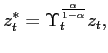
In this model, firms own their own capital. The firm cannot adjust its capital stock within the period. It can only change its stock of capital over time by varying the rate of investment. In all other respects the problem of intermediate good firms is the same as before. In particular, they face the same demand curve, (2), production technology, (4)-(8), and Calvo-style pricing frictions, including the updating rule given by (9).
The technology for accumulating physical capital by intermediate
good firm ![]() is given by
is given by
The present discounted value of the ![]() intermediate good's net cash flow is given by:
intermediate good's net cash flow is given by:
![$\displaystyle E_{t}\sum_{j=0}^{\infty}\beta^{j}\upsilon_{t+j}\left\{ P_{t+j}(i)y_{t+j} (i)-P_{t+j}R_{t+j}w_{t+j}(i)h_{t}(i)-P_{t+j}\Upsilon_{t+j}^{-1}\left[ I_{t+j}(i)+a\left( u_{t+j}(i)\right) \bar{K}(i)_{t+j}\right] \right\} .$](img225.gif)
|
(21) |
Time ![]() net cash flow equals sales, less labor
costs (inclusive of interest charges) less the costs associated
with capital utilization and capital accumulation.
net cash flow equals sales, less labor
costs (inclusive of interest charges) less the costs associated
with capital utilization and capital accumulation.
The sequence of events as it pertains to the ![]() firm is as follows. At the beginning of period
firm is as follows. At the beginning of period
![]() the firm has a given stock of physical
capital,
the firm has a given stock of physical
capital,
![]() . After observing the
technology shocks, the firm sets its price,
. After observing the
technology shocks, the firm sets its price, ![]() subject to the Calvo-style frictions described above. The firm also
makes its investment and capital utilization decisions,
subject to the Calvo-style frictions described above. The firm also
makes its investment and capital utilization decisions, ![]() and
and ![]() respectively. The
time
respectively. The
time ![]() monetary policy shock then occurs and the
demand for the firm's product is realized. The firm then purchases
labor to satisfy the demand for its output. Subject to these timing
and other constraints, the problem of the firm is to choose prices,
employment, the level of investment and utilization to maximize net
discounted cash flow.
monetary policy shock then occurs and the
demand for the firm's product is realized. The firm then purchases
labor to satisfy the demand for its output. Subject to these timing
and other constraints, the problem of the firm is to choose prices,
employment, the level of investment and utilization to maximize net
discounted cash flow.
2.3. Implications for Inflation
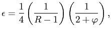
The equations which characterize equilibrium for the homogenous and firm-specific capital model are identical except for the equation which characterizes aggregate inflation dynamics. This equation is of the form:
| (22) |
where
and ![]() is the first difference operator. The
information set
is the first difference operator. The
information set
![]() includes the current realization
of the technology shocks, but not the current realization of the
innovation to monetary policy. The variable
includes the current realization
of the technology shocks, but not the current realization of the
innovation to monetary policy. The variable ![]() denotes the economy-wide average marginal cost of production, in
units of the final good.
denotes the economy-wide average marginal cost of production, in
units of the final good.
In ACEL (2004) we establish the following19:
Proposition 1 (i) In the homogeneous capital model,
![]() (ii) In the firm-specific capital
model,
(ii) In the firm-specific capital
model, ![]() is a particular non-linear function of
the parameters of the model.
is a particular non-linear function of
the parameters of the model.
We parameterize the firm-specific and homogeneous capital model
in terms of ![]() rather than
rather than ![]() Consequently, the list of parameters for the two
models remains identical. Given values for these parameters, the
two models are observationally equivalent with respect to aggregate
prices and quantities. This means that we do not need to take a
stand on which version of the model we are working with at the
estimation stage of our analysis.
Consequently, the list of parameters for the two
models remains identical. Given values for these parameters, the
two models are observationally equivalent with respect to aggregate
prices and quantities. This means that we do not need to take a
stand on which version of the model we are working with at the
estimation stage of our analysis.
3. Econometric Methodology
We employ a variant of the limited information strategy used in
CEE (2005) (see also Rotemberg and Woodford (1997)). Define the ten
dimensional vector, ![]() :
:
![$\displaystyle \underset{10\times1}{\underbrace{Y_{t}}}=\left( \begin{array}[c]{c} \Delta\ln\text{(relative price of investment}_{t}\text{)}\\ \Delta\ln\text{(}GDP_{t}/\text{Hours}_{t}\text{)}\\ \Delta\ln\text{(}GDP\text{ deflator}_{t}\text{)}\\ \text{Capacity Utilization}_{t}\\ \ln\text{(Hours}_{t}\text{)}\\ \ln\text{(}GDP_{t}/\text{Hours}_{t}\text{)}-\ln\text{(}W_{t}/P_{t}\text{)}\\ \ln\text{(}C_{t}/GDP_{t}\text{)}\\ \ln\text{(}I_{t}/GDP_{t}\text{)}\\ \text{Federal Funds Rate}_{t}\\ \ln(GDP\text{ deflator}_{t})+\ln\text{(}GDP_{t}\text{)}-\ln\text{(} MZM_{t}\text{)} \end{array} \right) =\left( \begin{array}[c]{c} \underset{1\times1}{\underbrace{\Delta p_{It}}}\\ \underset{1\times1}{\underbrace{\Delta a_{t}}}\\ \underset{6\times1}{\underbrace{Y_{1t}}}\\ \underset{1\times1}{\underbrace{R_{t}}}\\ \underset{1\times1}{\underbrace{Y_{2t}}} \end{array} \right)$](img244.gif)
|
(23) |
We embed our identifying assumptions as restrictions on the parameters of the following reduced form VAR:
| (24) | ||
where ![]() is a
is a ![]() -ordered
polynomial in the lag operator,
-ordered
polynomial in the lag operator, ![]() The "
fundamental" economic shocks,
The "
fundamental" economic shocks,
![]() are related to
are related to ![]() as follows:
as follows:
| (25) |
where ![]() is a square matrix and
is a square matrix and ![]() is the identity matrix. We assume that
is the identity matrix. We assume that
![]() is a martingale difference
stochastic process, so that we allow for the presence of
conditional heteroscedasticity.20 We require
is a martingale difference
stochastic process, so that we allow for the presence of
conditional heteroscedasticity.20 We require ![]() and the
and the ![]() column of
column of ![]()
![]() to calculate the dynamic response of
to calculate the dynamic response of
![]() to a disturbance in the
to a disturbance in the ![]() fundamental shock,
fundamental shock,
![]()
According to our economic model, the variables in ![]() defined in (23), are stationary
stochastic processes. We partition
defined in (23), are stationary
stochastic processes. We partition
![]() conformably with the
partitioning of
conformably with the
partitioning of ![]()
![$\displaystyle \varepsilon_{t}=\left( \begin{array}[c]{ccccc} \underset{1\times1}{\underbrace{\varepsilon_{\Upsilon,t}}} & \underset{1\times 1}{\underbrace{\varepsilon_{z,t}}} & \underset{1\times 6}{\underbrace{\varepsilon_{1t}^{\prime}}} & \underset{1\times 1}{\underbrace{\varepsilon_{M,t}}} & \underset{1\times 1}{\underbrace{\varepsilon_{2t}}} \end{array} \right) ^{\prime}.$](img269.gif)
|
(26) |
Here,
![]() is the innovation to a
neutral technology shock,
is the innovation to a
neutral technology shock,
![]() is the innovation
in capital-embodied technology, and
is the innovation
in capital-embodied technology, and
![]() is the monetary policy
shock.
is the monetary policy
shock.
3.1. Identification of Impulse Responses
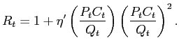
We assume that policy makers set the interest rate so that the following rule is satisfied:
| (27) |
where
![]() is the monetary policy
shock and
is the monetary policy
shock and
![]() is a constant. We interpret
(27) as a reduced form Taylor rule. To ensure
identification of the monetary policy shock, we assume
is a constant. We interpret
(27) as a reduced form Taylor rule. To ensure
identification of the monetary policy shock, we assume ![]() is linear,
is linear,
![]() contains
contains ![]()
![]() and the only date
and the only date ![]() variables in
variables in
![]() are {
are {
![]() }. Finally,
we assume that
}. Finally,
we assume that
![]() is orthogonal to
is orthogonal to
![]()
As in Fisher (2006), we assume that innovations to technology (both neutral and capital-embodied) are the only shocks which affect the level of labor productivity in the long run. In addition, we assume that capital embodied technology shocks are the only shocks that affect the price of investment goods relative to consumption goods in the long run. These assumptions are satisfied in our model.
To compute the responses of ![]() to
to
![]()
![]() and
and
![]() we require estimates of
the parameters in
we require estimates of
the parameters in ![]() as well as the
as well as the
![]()
![]() and
and
![]() columns of
columns of ![]() We
obtain these estimates using a suitably modified variant of the
instrumental variables strategy proposed by Shapiro and Watson
(1988). See ACEL (2004) for further details.
We
obtain these estimates using a suitably modified variant of the
instrumental variables strategy proposed by Shapiro and Watson
(1988). See ACEL (2004) for further details.
4. Estimation Results Based on a Structural Vector Autoregression
In this section we describe the dynamic response of the economy to monetary policy shocks, neutral technology shocks and capital embodied shocks. In addition, we discuss the quantitative contribution of these shocks to the cyclical fluctuations in aggregate economic activity. In the first subsection we describe the data used in the analysis. In the second and third subsections we discuss the impulse response functions and the importance of the shocks to aggregate fluctuations.
4.1. Data
With the exception of the price of investment and of monetary
transactions balances, all data were taken from the FRED Database
available through the Federal Reserve Bank of St. Louis.21 The
price of investment corresponds to the 'total investment' series
constructed and used in Fisher (2006).22 Our measure of
transactions balances, ![]() was obtained from the
Federal Reserve Bank of St. Louis's online database. Our data are
quarterly, and the sample period is 1982:1-2008:3.23
was obtained from the
Federal Reserve Bank of St. Louis's online database. Our data are
quarterly, and the sample period is 1982:1-2008:3.23
We work with the monetary aggregate, ![]() for the
following reasons. First,
for the
following reasons. First, ![]() is constructed
to be a measure of transactions balances, so it is a natural
empirical counterpart to our model variable,
is constructed
to be a measure of transactions balances, so it is a natural
empirical counterpart to our model variable, ![]() Second, our statistical procedure requires that the
velocity of money is stationary. The velocity of
Second, our statistical procedure requires that the
velocity of money is stationary. The velocity of ![]() is reasonably characterized as being stationary. The
stationarity assumption is more problematic for the velocity of
aggregates like the base,
is reasonably characterized as being stationary. The
stationarity assumption is more problematic for the velocity of
aggregates like the base, ![]() and
and ![]()
4.2. Estimated Impulse Response Functions
In this subsection we discuss our estimates of the dynamic
response of ![]() to monetary policy and technology
shocks. To obtain these estimates we set
to monetary policy and technology
shocks. To obtain these estimates we set ![]() the
number of lags in the VAR, to 4. Various
indicators suggest that this value of
the
number of lags in the VAR, to 4. Various
indicators suggest that this value of ![]() is large
enough to adequately capture the dynamics in the data. For example,
the Akaike, Hannan-Quinn and Schwartz criteria support a choice of
is large
enough to adequately capture the dynamics in the data. For example,
the Akaike, Hannan-Quinn and Schwartz criteria support a choice of
![]() 2, 1,
respectively.24 We also compute the multivariate
Portmanteau (Q) statistic to test the null hypothesis of zero
serial correlation up to lag
2, 1,
respectively.24 We also compute the multivariate
Portmanteau (Q) statistic to test the null hypothesis of zero
serial correlation up to lag ![]() in the VAR
disturbances. We consider
in the VAR
disturbances. We consider ![]() 6, 8, 10. The test
statistics are, respectively,
6, 8, 10. The test
statistics are, respectively, ![]() 475, 680, 880. Using
conventional asymptotic sampling theory, these
475, 680, 880. Using
conventional asymptotic sampling theory, these ![]() statistics all have a
statistics all have a ![]() -value very close to zero,
indicating a rejection of the null hypothesis. However, we find
evidence that the asymptotic sampling theory rejects the null
hypothesis too often. When we simulate the
-value very close to zero,
indicating a rejection of the null hypothesis. However, we find
evidence that the asymptotic sampling theory rejects the null
hypothesis too often. When we simulate the ![]() statistic using repeated artificial data sets generated from our
estimated VAR, we find that the
statistic using repeated artificial data sets generated from our
estimated VAR, we find that the ![]() -values of our
-values of our
![]() statistics are 97, 87, 90 and 95 percent, respectively. For these calculations, each
artificial data set is of length equal to that of our actual
sample, and is generated by bootstrap sampling from the fitted
disturbances in our estimated VAR. On this basis we do not strongly
reject the null hypothesis that the disturbance terms in a VAR with
statistics are 97, 87, 90 and 95 percent, respectively. For these calculations, each
artificial data set is of length equal to that of our actual
sample, and is generated by bootstrap sampling from the fitted
disturbances in our estimated VAR. On this basis we do not strongly
reject the null hypothesis that the disturbance terms in a VAR with
![]() are serially uncorrelated.
are serially uncorrelated.
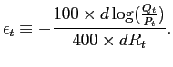
Figure 1 displays the response of the variables in our analysis to a one standard deviation monetary policy shock (roughly 30 basis points). In each case, there is a solid line in the center of a gray area. The gray area represents a 95 percent confidence interval, and the solid line represents the point estimates.25 Except for inflation and the interest rate, all variables are expressed in percent terms. So, for example, the peak response of output is about 0.15 percent. The Federal Funds rate is expressed in units of percentage points, at an annual rate. Inflation is expressed in units of percentage points, at a quarterly rate.
Six features of Figure 1 are worth noting. First, the effect of a policy shock on the money growth rate and the interest rate is completed within roughly one year. Other quantity variables respond over a longer period of time. Second, there is a significant liquidity effect, i.e. the interest rate and money growth move in opposite directions after a policy shock. Third, inflation responds very weakly to the policy shock. Fourth, output, consumption, investment, hours worked and capacity utilization all display hump-shaped responses. With the exception of hours worked, the peak response in these aggregates occurs roughly one year after the shock. The hump shaped response in hours worked is more drawn out, with the peak occurring after approximately two years. Fifth, velocity co-moves with the interest rate, with both initially falling in response to a monetary policy shock, and then rising. Sixth, the real wage does not respond significantly to a monetary policy shock, but after a delay the price of investment does.
Figure 2 displays the response of the variables in our analysis
to a positive, one standard deviation shock in neutral technology,
![]() By construction, the impact of this
technology shock on output, labor productivity, consumption,
investment and the real wage can be permanent. Because the roots of
our estimated VAR are stable, the impact of a neutral technology
shock on the variables whose levels appear in
By construction, the impact of this
technology shock on output, labor productivity, consumption,
investment and the real wage can be permanent. Because the roots of
our estimated VAR are stable, the impact of a neutral technology
shock on the variables whose levels appear in ![]() must be temporary. These variables are the Federal
Funds rate, capacity utilization, hours worked, velocity and
inflation.
must be temporary. These variables are the Federal
Funds rate, capacity utilization, hours worked, velocity and
inflation.
According to Figure 2 a positive, neutral technology shock leads to a persistent rise in output with a peak rise of roughly 0.35 percent over the period displayed. In addition, hours worked, investment and consumption rise in response to the technology shock. These rises are only marginally statistically significant. Finally notice that a neutral technology shock leads to an initial sharp fall in the inflation rate.26. Overall, these effects are broadly consistent with what a student of real business cycle models might expect.
Figure 3 displays the response of the variables in our analysis
to a one standard deviation positive capital-embodied technology
shock,
![]() This shock leads
to statistically significant rises in output, hours worked,
capacity utilization, investment and the federal funds rate. At the
same time, it leads to an initial fall in the price of investment
of roughly 0.2 percent, followed by an ongoing
significant decline. Finally, the shock also leads a marginally
significant decline in real wages.
This shock leads
to statistically significant rises in output, hours worked,
capacity utilization, investment and the federal funds rate. At the
same time, it leads to an initial fall in the price of investment
of roughly 0.2 percent, followed by an ongoing
significant decline. Finally, the shock also leads a marginally
significant decline in real wages.
4.3. The Contribution of Monetary Policy and Technology Shocks to Aggregate Fluctuations
We now briefly discuss the contribution of monetary policy and
technology shocks to cyclical fluctuations in economic activity.
Table 1 summarizes the contribution of the three shocks to the
variables in our analysis. We define business cycle frequencies as
the components of a time series with periods of 8 to 32 quarters.
The columns in Table 1 report the fraction of the variance in the
cyclical frequencies accounted for by our three shocks. Each row
corresponds to a different variable. Using the techniques described
in Christiano and Fitzgerald (2003), we calculate the fractions as
follows. Let
![]() denote the spectral density at
frequency
denote the spectral density at
frequency ![]() of a given variable, when only
shock
of a given variable, when only
shock ![]() is active. That is, the variance of all
shocks in
is active. That is, the variance of all
shocks in
![]() apart from the
apart from the ![]() are set to zero and the variance of the
are set to zero and the variance of the ![]() shock in
shock in
![]() is set to unity. Let
is set to unity. Let
![]() denote the corresponding spectral
density when the variance of each element of
denote the corresponding spectral
density when the variance of each element of
![]() is set to unity. The
contribution of shock
is set to unity. The
contribution of shock ![]() to variance in the business
cycle frequencies is then defined as:
to variance in the business
cycle frequencies is then defined as:
Our estimate of the spectral density is the one implied by our estimated VAR.27 Numbers in parentheses are the standard errors, which we estimate by bootstrap methods. Finally, the fraction of the variance accounted for by all three shocks is just the sum of the individual fractions of the variance.
Table 1 shows that the three shocks together account for a substantial portion of the cyclical variance in the aggregate quantities. For example, they account for roughly 60 percent of the variation in aggregate output, with the capital-embodied technology shock playing the largest role. Indeed the capital-embodied technology shock is the largest contributor to the cyclical variation in all of the variables included in the VAR. Intriguingly, the capital embodied technology shock accounts for nearly 30% of the cyclical variation in the real wage, a variable whose cyclical variation is typically difficult to account for empirically.
5. Estimation Results for the Equilibrium Model
In this section we discuss the estimated parameter values. In addition, we assess the ability of the estimated model to account for the impulse response functions discussed in Section 4.
5.1. Benchmark Model Parameter Estimates
We partition the parameters of the model into three groups. The
first group of parameters,
![]() is:
is:
The second group of parameters,
![]() pertain to the 'non-stochastic
part' of the model:
pertain to the 'non-stochastic
part' of the model:
The third set of parameters,
![]() pertain to the stochastic part of
the model:
pertain to the stochastic part of
the model:
We estimate the values of ![]() and
and
![]() and set the values of
and set the values of ![]() a priori. We assume
a priori. We assume
![]() , which implies a steady
state annualized real interest rate of 3 percent. We
set
, which implies a steady
state annualized real interest rate of 3 percent. We
set
![]() which corresponds to a steady
state share of capital income equal to roughly 36
percent.28 We set
which corresponds to a steady
state share of capital income equal to roughly 36
percent.28 We set
![]() , which implies an annual rate
of depreciation on capital equal to 10 percent. This value of
, which implies an annual rate
of depreciation on capital equal to 10 percent. This value of
![]() is roughly equal to the estimate
reported in Christiano and Eichenbaum (1992). The parameter,
is roughly equal to the estimate
reported in Christiano and Eichenbaum (1992). The parameter,
![]() is set to guarantee that profits are
zero in steady state. As in CEE (2005), we set the parameter,
is set to guarantee that profits are
zero in steady state. As in CEE (2005), we set the parameter,
![]() to 1.05. We set
the parameter
to 1.05. We set
the parameter ![]() to one.
to one.
The steady state growth of real per capita GDP, ![]() is given by
is given by
Given an estimate of ![]() and
and
![]() we use this equation to
estimate
we use this equation to
estimate ![]() We use data over the sample period
1959II - 2001IV, the sample period in ACEL (2005), to estimate the
parameters
We use data over the sample period
1959II - 2001IV, the sample period in ACEL (2005), to estimate the
parameters
![]() and
and ![]() If we use the sample period 1982:1-2008:3, then the implied point
estimate of
If we use the sample period 1982:1-2008:3, then the implied point
estimate of ![]() is less than one, a value that
seems implausible to us. It seems reasonable to extend the sample
back in time because the value of
is less than one, a value that
seems implausible to us. It seems reasonable to extend the sample
back in time because the value of ![]() should
not be affected by any change in the monetary policy regime that
occurred in the early 1980's. For comparability with ACEL (2005) we
stopped the sample period at 2001IV.29With these
considerations in mind, we set the parameter
should
not be affected by any change in the monetary policy regime that
occurred in the early 1980's. For comparability with ACEL (2005) we
stopped the sample period at 2001IV.29With these
considerations in mind, we set the parameter
![]() to 1.0042.
At an annualized rate, this value is equal to the negative of the
average growth rate of the price of investment relative to the GDP
deflator which fell at an annual average rate of 1.68 percent over the ACEL (2005) sample period. The average
growth rate of per capita GDP in the ACEL (2005) sample period is
to 1.0042.
At an annualized rate, this value is equal to the negative of the
average growth rate of the price of investment relative to the GDP
deflator which fell at an annual average rate of 1.68 percent over the ACEL (2005) sample period. The average
growth rate of per capita GDP in the ACEL (2005) sample period is
![]() Solving the previous
equation for
Solving the previous
equation for ![]() yields
yields
![]() which is the value of
which is the value of
![]() we use in our analysis.30 We
set the average growth rate of money,
we use in our analysis.30 We
set the average growth rate of money, ![]() equal
to 1.017.31 This value corresponds to the
average quarterly growth rate of money
equal
to 1.017.31 This value corresponds to the
average quarterly growth rate of money ![]() over the
ACEL (2005) sample period.
over the
ACEL (2005) sample period.
We set the parameters
![]() and
and ![]() to
0.45 and 0.036, respectively.
The value of
to
0.45 and 0.036, respectively.
The value of
![]() corresponds to the average value
of
corresponds to the average value
of
![]() in the ACEL (2005) sample
period, where
in the ACEL (2005) sample
period, where ![]() is measured by
is measured by ![]() We chose
We chose ![]() so that in conjunction
with the other parameter values of our model, the steady state
value of
so that in conjunction
with the other parameter values of our model, the steady state
value of ![]() is 0.025. This
corresponds to the percent of value-added in the finance, insurance
and real estate industry (see Christiano, Motto, and Rostagno
(2004)).
is 0.025. This
corresponds to the percent of value-added in the finance, insurance
and real estate industry (see Christiano, Motto, and Rostagno
(2004)).
The row labeled 'benchmark' in Table 2 summarizes our point
estimates of the parameters in the vector
![]() Standard errors are reported in
parentheses. The lower bound of unity is binding on
Standard errors are reported in
parentheses. The lower bound of unity is binding on
![]() So we simply set
So we simply set
![]() to 1.01 when we
estimate the model. However, the estimation criterion displays very
little curvature with respect to
to 1.01 when we
estimate the model. However, the estimation criterion displays very
little curvature with respect to
![]() . When we individually test the
hypotheses that
. When we individually test the
hypotheses that
![]() is 1.05 or
1.20 against the null that
is 1.05 or
1.20 against the null that
![]() we obtain a chi-square
statistic equal to 0.01 and 0.2, respectively, with associated probability values 0.0002
and 0.024, respectively. So we cannot clearly
reject either hypothesis. Tables 2 and 3 report point estimates for
we obtain a chi-square
statistic equal to 0.01 and 0.2, respectively, with associated probability values 0.0002
and 0.024, respectively. So we cannot clearly
reject either hypothesis. Tables 2 and 3 report point estimates for
![]() and
and ![]() when
we re-estimate the model setting
when
we re-estimate the model setting
![]() to 1.05 and
1.20.
to 1.05 and
1.20.
Our point estimate of ![]() implies that wage
contracts are re-optimized, on average, once every 4.5 quarters. To interpret our point estimate of
implies that wage
contracts are re-optimized, on average, once every 4.5 quarters. To interpret our point estimate of ![]() recall that in the homogeneous capital model,
recall that in the homogeneous capital model,
![]() So our point estimate of
So our point estimate of ![]() implies a value of
implies a value of
![]() equal to
equal to ![]() This
implies that firms re-optimize prices roughly every 9.36 quarters (see Table 4). This value is much larger than
the value used by Golosov and Lucas (2007) who calibrate their
model to micro data to ensure that the firms re-optimize prices on
average once every 1.5 quarters.
This
implies that firms re-optimize prices roughly every 9.36 quarters (see Table 4). This value is much larger than
the value used by Golosov and Lucas (2007) who calibrate their
model to micro data to ensure that the firms re-optimize prices on
average once every 1.5 quarters.
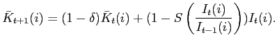
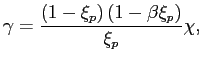
Table 4 shows that if we adopt the assumption that capital is firm-specific, then our estimates imply that firms re-optimize prices on average once every 1.8 quarters.32 So the assumption that capital is firm-specific has a very large impact on inference about the frequency at which firms re-optimize price.
To interpret the estimated value of
![]() , we consider the homogeneous
capital model. Linearizing the household's first order condition
for capital utilization about steady state yields:
, we consider the homogeneous
capital model. Linearizing the household's first order condition
for capital utilization about steady state yields:
According to this expression,
![]() , equal to 0.08 of a percent, is the elasticity of capital utilization
with respect to the rental rate of capital. Our estimate of
, equal to 0.08 of a percent, is the elasticity of capital utilization
with respect to the rental rate of capital. Our estimate of
![]() is larger than the value
estimated by CEE (2005) and indicates that it is relatively costly
for firms to vary the utilization of capital.
is larger than the value
estimated by CEE (2005) and indicates that it is relatively costly
for firms to vary the utilization of capital.
Our point estimate of the habit parameter ![]() is 0.76. This value is reasonably close to the
point estimate of 0.66, reported in CEE (2005)
and the value of 0.7 reported in Boldrin, Christiano,
and Fisher (2001). The latter authors argue that the ability of
standard general equilibrium models to account for the equity
premium and other asset market statistics is considerably enhanced
by the presence of habit formation in preferences.
is 0.76. This value is reasonably close to the
point estimate of 0.66, reported in CEE (2005)
and the value of 0.7 reported in Boldrin, Christiano,
and Fisher (2001). The latter authors argue that the ability of
standard general equilibrium models to account for the equity
premium and other asset market statistics is considerably enhanced
by the presence of habit formation in preferences.
We now discuss our point estimate of
![]() Suppose we denote by
Suppose we denote by
![]() the shadow price of one
unit of
the shadow price of one
unit of
![]() in terms of output. The
variable
in terms of output. The
variable
![]() is what the price of
installed capital would be in the homogeneous capital model if
there were a market for
is what the price of
installed capital would be in the homogeneous capital model if
there were a market for
![]() at the beginning of period
at the beginning of period
![]() Proceeding as in CEE (2005), it is
straightforward to show that the household's first order condition
for investment implies:
Proceeding as in CEE (2005), it is
straightforward to show that the household's first order condition
for investment implies:
![$\displaystyle \hat{\imath}_{t}=\hat{\imath}_{t-1}+\frac{1}{S^{\prime\prime}}\sum _{j=0}^{\infty}\beta^{j}E[\hat{P}_{k^{\prime},t+j}\vert\Omega_{t}]. $](img451.gif)
According to this expression,
![]() is the elasticity of
investment with respect to a one percent temporary increase in the
current price of installed capital. Our point estimate implies that
this elasticity is equal to 0.66. The more
persistent is the change in the price of capital, the larger is the
percentage change in investment. This property holds because
adjustment costs induce agents to be forward looking.
is the elasticity of
investment with respect to a one percent temporary increase in the
current price of installed capital. Our point estimate implies that
this elasticity is equal to 0.66. The more
persistent is the change in the price of capital, the larger is the
percentage change in investment. This property holds because
adjustment costs induce agents to be forward looking.
Table 3 reports the estimated values of the parameters pertaining to the stochastic part of the model. With these values, the laws of motion for the neutral and capital-embodied technology shocks are:
Numbers in parentheses are standard errors. Our estimates imply
that a one-standard deviation neutral technology shock drives
![]() up by 0.17 percent
in the period of the shock and by 0.29
up by 0.17 percent
in the period of the shock and by 0.29
![]() percent in the long run. A
one-standard-deviation shock to embodied technology drives
percent in the long run. A
one-standard-deviation shock to embodied technology drives
![]() up by 0.21
percent immediately and by 0.47 percent in the
long run. Our estimates imply that shocks to neutral technology
exhibit a high degree of serial correlation, while shocks to
capital-embodied technology do not.
up by 0.21
percent immediately and by 0.47 percent in the
long run. Our estimates imply that shocks to neutral technology
exhibit a high degree of serial correlation, while shocks to
capital-embodied technology do not.
It is interesting to compare our results for
![]() with the ones reported in
Prescott (1986), who estimates the properties of the technology
shock process using the Solow residual. He finds that the shock is
roughly a random walk, and its growth rate has a standard deviation
of roughly
with the ones reported in
Prescott (1986), who estimates the properties of the technology
shock process using the Solow residual. He finds that the shock is
roughly a random walk, and its growth rate has a standard deviation
of roughly ![]() percent.33 By contrast, our
estimates imply that the unconditional standard deviation of the
growth rate of neutral technology is roughly
percent.33 By contrast, our
estimates imply that the unconditional standard deviation of the
growth rate of neutral technology is roughly ![]()
![]() /
/
![]() ) percent. So we find
that technology shocks are substantially less volatile but more
persistent than those estimated by Prescott. In principle, these
differences reflect two factors. First, from the perspective of our
model, Prescott's estimate of technology confounds technology with
variable capital utilization. Second, our analysis is based on
different data sets and different identifying assumptions than
Prescott's.
) percent. So we find
that technology shocks are substantially less volatile but more
persistent than those estimated by Prescott. In principle, these
differences reflect two factors. First, from the perspective of our
model, Prescott's estimate of technology confounds technology with
variable capital utilization. Second, our analysis is based on
different data sets and different identifying assumptions than
Prescott's.
5.2. Impulse Responses
The dotted lines in Figures 1 through 3 display the impulse response functions of the estimated model to monetary policy, neutral technology shocks and capital-embodied shocks, respectively. Recall that the solid lines and the associated confidence intervals (the gray areas) pertain to the impulse response functions from the estimated, identified VARs.
5.2.1. Response to a Monetary Policy Shock
We begin by discussing the model's performance with respect to a monetary policy shock (see Figure 1). First, consistent with results in CEE (2005), the model does well at accounting for the dynamic response of the U.S. economy to a monetary policy shock. Most (but not all) of the model responses lie within the two-standard deviation confidence interval computed from the data. This is true even though firms in the firm-specific capital version of the model change prices on average once every 1.8 quarters.
Second, the model generates a very persistent response in output. The peak effect occurs roughly one year after the shock. The output response is positive for over three years. Third, the model accounts for the dynamic response of the interest rate to a monetary policy shock. Consistent with the data, an expansionary monetary policy shock induces a sharp decline in the interest rate which then returns to its pre-shock level within a year. The model does not account for the overshooting pattern of the interest rate in the data. The growth rate of transactions balances rises for a brief period of time after the policy shock, but then quickly reverts to its pre-shock level. But the model does not account for the overshooting pattern seen in transaction balances. Figure 1 shows that the effects of a policy shock on aggregate economic activity persist beyond the effects on the policy variable itself, regardless of whether the policy variable is measured as the interest rate or the money supply. This property reflects the strong internal propagation mechanisms in the model.
Fourth, as in the data, the real wage remains essentially unaffected by the policy shock. Fifth, consumption, investment, and hours worked exhibit persistent, hump-shaped rises that are consistent with our VAR-based estimates. Sixth, consistent with the data, velocity falls after the expansionary policy shock. This fall reflects the rise in money demand associated with the initial fall in the interest rate. However this fall is nearly as strong as the VAR based response of velocity to a monetary policy shock. Seventh, by construction, the relative price of investment is not affected by a policy shock in the model. At least for the first two years after the policy shock, this lack of response is consistent with the response of the relative price of investment to a policy shock in the identified VAR. It is not consistent with the rise in that price in the third year after the shock. Finally, capacity utilization in the model rises by only a very small amount, and understates the estimated rise in the data.
Overall the response of the model to a monetary policy shock is quite similar to the response of the estimated model in CEE (2005). This result holds even though the models are estimated over very different sample periods. The main difference is that the size of the monetary policy shock is almost twice as large as in ACEL (2005). But conditional on a given monetary policy shock, the transmission mechanism in the two estimated models is very similar.
5.2.2. Response to a Neutral Technology Shock
We now discuss the model's performance with respect to a neutral technology shock (see Figure 2). First, the model does well at accounting for the dynamic response of the U.S. economy to a neutral technology shock. Specifically, the model accounts for the rise in aggregate output, hours worked, investment, consumption and the real wage. However, the model does not capture the extent of the fall in inflation that occurs immediately after the shock.
5.2.3. Response to a Capital Embodied Technology Shock
We now discuss the model's performance with respect to a capital-embodied technology shock (see Figure 3). The model does very well in accounting for the response of the U.S. economy to this shock, except that it does not account for the rises in capacity utilization and the federal funds rate that occur after the capital-embodied technology shock. In addition money growth is high relative to the estimated response from the VAR. To see the importance of monetary policy in the transmission of capital embodied technology shocks, we compute the response of the model economy to a positive, capital embodied technology shock under the assumption that money growth remains unchanged from its steady state level. We find that output and hours worked rise by much less, while inflation falls compared to what happens when monetary policy is accommodative. We conclude that the model requires accommodative monetary policy to match the expansionary effects of a positive capital embodied technology shock.
6. The Key Features of the Model
In this section we discuss the features of the data driving our estimates of the parameters determining the implications of the firm-specific and homogeneous capital models for the frequency at which firms re-optimize prices.
Our point estimate of ![]() (0.014) implies that a temporary one percent change in
marginal cost results in only a 0.02 percent change
in the aggregate price level.34The small value of
(0.014) implies that a temporary one percent change in
marginal cost results in only a 0.02 percent change
in the aggregate price level.34The small value of ![]() lies at the heart of the tension between the micro and
macro implications of the homogeneous capital model.
lies at the heart of the tension between the micro and
macro implications of the homogeneous capital model.
We now argue that any reasonable estimate of ![]() must be low. In Figure 4a we plot
must be low. In Figure 4a we plot
![]() against our
measure of the log of marginal cost,
against our
measure of the log of marginal cost,
![]() .35 The distribution of
.35 The distribution of
![]() is at best
weakly related to the magnitude of
is at best
weakly related to the magnitude of
![]() 36 The relatively flat
curve in Figure 4a has a slope equal to our point estimate of
36 The relatively flat
curve in Figure 4a has a slope equal to our point estimate of
![]() (0.014).
Significantly, this curve passes through the central tendency of
the data. The steeper curve in Figure 4a is drawn for a value of
(0.014).
Significantly, this curve passes through the central tendency of
the data. The steeper curve in Figure 4a is drawn for a value of
![]() equal to 0.68 a value
which implies that in the homogeneous capital model firms change
prices roughly once every 1.8 quarters. Figure
4a shows that raising
equal to 0.68 a value
which implies that in the homogeneous capital model firms change
prices roughly once every 1.8 quarters. Figure
4a shows that raising ![]() to 0.68 leads to a drastic deterioration in fit.
to 0.68 leads to a drastic deterioration in fit.
Equation (22) implies that the
magnitude of the residuals from the lines in Figure 4a cannot be
used as a formal measure of model fit. We should focus on the size
of residuals when the data are replaced by their projection onto
date ![]() information, because then (22) implies that least squares consistently
recovers the true value of
information, because then (22) implies that least squares consistently
recovers the true value of ![]() . Figure 4b is
the analog to Figure 4a, with variables replaced by their
projection onto
. Figure 4b is
the analog to Figure 4a, with variables replaced by their
projection onto
![]() Figures 4a and 4b are very similar so that our conclusions are
unchanged: the data on inflation and marginal cost suggest that
Figures 4a and 4b are very similar so that our conclusions are
unchanged: the data on inflation and marginal cost suggest that
![]() is small.37
is small.37
The low estimated value of ![]() provides a
different perspective on the inflation inertia puzzle, particularly
the weak response of inflation to monetary policy shocks. Solving
(22) forward we obtain
provides a
different perspective on the inflation inertia puzzle, particularly
the weak response of inflation to monetary policy shocks. Solving
(22) forward we obtain
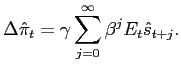
|
(28) |
This relation makes clear why many authors incorporate features
like variable capital utilization and sticky wages into their
models. These features can reduce the response of expected marginal
cost to shocks.38 Relation (28) reveals another way to account for inflation
inertia: assign a small value to ![]() The evidence
in Figure 4a and 4b indicates that a small value of
The evidence
in Figure 4a and 4b indicates that a small value of ![]() must be part of any successful resolution of the
inflation inertia puzzle.
must be part of any successful resolution of the
inflation inertia puzzle.
A low value of ![]() is clearly a problem
for the homogeneous capital model. This is because the model then
implies that firms re-optimize prices very infrequently, e.g., at
intervals of roughly 9.5 quarters.39 So
to get the macro data right (i.e., a low
is clearly a problem
for the homogeneous capital model. This is because the model then
implies that firms re-optimize prices very infrequently, e.g., at
intervals of roughly 9.5 quarters.39 So
to get the macro data right (i.e., a low ![]() we must make assumptions about the frequency at which firms
re-optimize prices that seem implausible in light of the micro
data. In contrast, suppose we adopt the more plausible assumption
that firms re-optimize prices on average once every 1.8 quarters. Then the homogeneous capital model implies
we must make assumptions about the frequency at which firms
re-optimize prices that seem implausible in light of the micro
data. In contrast, suppose we adopt the more plausible assumption
that firms re-optimize prices on average once every 1.8 quarters. Then the homogeneous capital model implies
![]() But this means that the model
gets the macro data wrong.
But this means that the model
gets the macro data wrong.
In the firm-specific capital model it is possible to reconcile
the low value of ![]() with a low value of
with a low value of
![]() This reflects two features of that
model. The first is that not all firms set prices at the same time
(i.e., 'staggered pricing'). The second is that capital is
firm-specific so that the only way a firm can adjust its capital
stock is by varying its investment over time. To understand the
role of these features, suppose there is an increase in the
quantity of money. Flexible price firms respond by increasing their
prices. Depending on how elastic demand is, these price increases
cause demand to shift away from flexible price firms and towards
the sticky price firms. Consequently, flexible price firms need
less capital services. If firms could trade physical capital,
capital would flow from flexible price firms to sticky price firms.
With firm-specific capital this flow cannot occur. To the extent
that flexible price firms cannot easily reduce capital utilization
rates, the shadow value of capital to flexible price firms
plummets. This fall acts like a decline in marginal cost and
reduces the incentive of flexible price firms to raise prices in
the first place. This mechanism is enhanced the more elastic is
demand and the less flexible is capital utilization. No doubt, the
assumption that capital is completely immobile between firms is
unrealistic. At the same time, anything which causes a firm's
marginal cost to be an increasing function of its output works in
the same direction as firm-specificity of capital.40
This reflects two features of that
model. The first is that not all firms set prices at the same time
(i.e., 'staggered pricing'). The second is that capital is
firm-specific so that the only way a firm can adjust its capital
stock is by varying its investment over time. To understand the
role of these features, suppose there is an increase in the
quantity of money. Flexible price firms respond by increasing their
prices. Depending on how elastic demand is, these price increases
cause demand to shift away from flexible price firms and towards
the sticky price firms. Consequently, flexible price firms need
less capital services. If firms could trade physical capital,
capital would flow from flexible price firms to sticky price firms.
With firm-specific capital this flow cannot occur. To the extent
that flexible price firms cannot easily reduce capital utilization
rates, the shadow value of capital to flexible price firms
plummets. This fall acts like a decline in marginal cost and
reduces the incentive of flexible price firms to raise prices in
the first place. This mechanism is enhanced the more elastic is
demand and the less flexible is capital utilization. No doubt, the
assumption that capital is completely immobile between firms is
unrealistic. At the same time, anything which causes a firm's
marginal cost to be an increasing function of its output works in
the same direction as firm-specificity of capital.40
The key parameter which governs the flexibility of capital
utilization is
![]() The logic in the previous
paragraph suggests that for a fixed value of
The logic in the previous
paragraph suggests that for a fixed value of ![]() , the larger is
, the larger is
![]() the lower is
the lower is ![]() But other things equal, a lower
But other things equal, a lower ![]() implies a higher
implies a higher ![]() These
observation suggest that for a given value of
These
observation suggest that for a given value of ![]()
![]() is a decreasing function of
is a decreasing function of
![]() In fact, our point estimate of
In fact, our point estimate of
![]() is large which helps explain why
the value of
is large which helps explain why
the value of ![]() implied by the firm-specific
model is low.
implied by the firm-specific
model is low.
What is it about the data that leads to a large (albeit
imprecise) point estimate for
![]() We recompute the impulse
responses implied by our model, holding all but one of the model
parameters at their estimated values. The exception is
We recompute the impulse
responses implied by our model, holding all but one of the model
parameters at their estimated values. The exception is
![]() which we set to 0.01. The new value of
which we set to 0.01. The new value of
![]() has two major effects on the
model impulse response functions. First, the responses of capital
utilization to both technology shocks are stronger. The responses
are so strong that, at several horizons, they lie substantially
outside the corresponding empirical confidence intervals. This
effect is particularly strong for a capital-embodied technology
shock. Also the model has difficulty in matching the rise in
output, measured net of capacity utilization costs, after a
capital-embodied technology shock. Basically capacity utilization
rises by such a large amount that it leads to a drag in output net
of capacity utilization costs. These two effects explain why our
estimation criterion settles on a high value of
has two major effects on the
model impulse response functions. First, the responses of capital
utilization to both technology shocks are stronger. The responses
are so strong that, at several horizons, they lie substantially
outside the corresponding empirical confidence intervals. This
effect is particularly strong for a capital-embodied technology
shock. Also the model has difficulty in matching the rise in
output, measured net of capacity utilization costs, after a
capital-embodied technology shock. Basically capacity utilization
rises by such a large amount that it leads to a drag in output net
of capacity utilization costs. These two effects explain why our
estimation criterion settles on a high value of
![]()
In Table 2 and 3 we report the results of estimating the model
subject to the constraint that
![]() is a small number, 0.01. (see the row labelled 'Low Cost of Varying Capacity
Utilization). Note that the point estimate rises from 0.014 to0.065, a value that is inconsistent with
the estimated value of
is a small number, 0.01. (see the row labelled 'Low Cost of Varying Capacity
Utilization). Note that the point estimate rises from 0.014 to0.065, a value that is inconsistent with
the estimated value of ![]() discussed in the
context of Figure 4. Table 4 shows that consistent with our
intuition, the homogeneous and firm-specific capital model now
yield very similar implications for the frequency with which firms
re-optimize prices, namely about once a year.
discussed in the
context of Figure 4. Table 4 shows that consistent with our
intuition, the homogeneous and firm-specific capital model now
yield very similar implications for the frequency with which firms
re-optimize prices, namely about once a year.
To verify our intuition about why our benchmark estimate of
![]() is high, we re-estimate the model
including only the responses to a monetary policy shock in the
criterion. We report our results in Tables 2, 3 and 4. Our point
estimate of
is high, we re-estimate the model
including only the responses to a monetary policy shock in the
criterion. We report our results in Tables 2, 3 and 4. Our point
estimate of
![]() falls from 11.42 to 3.93. The lower value of
falls from 11.42 to 3.93. The lower value of
![]() allows the model to better
capture the estimated rise in capital utilization that occurs after
a monetary policy shock, without paying a penalty for a
counterfactually large rise in capacity utilization and a fall in
output after a capital-embodied technology shock. This result
reconciles our findings with those reported in CEE (2005) who
report a low estimated value of
allows the model to better
capture the estimated rise in capital utilization that occurs after
a monetary policy shock, without paying a penalty for a
counterfactually large rise in capacity utilization and a fall in
output after a capital-embodied technology shock. This result
reconciles our findings with those reported in CEE (2005) who
report a low estimated value of
![]() based on an estimation criterion
that includes only the responses to a monetary policy shock.
based on an estimation criterion
that includes only the responses to a monetary policy shock.
To pursue our intuition about the benchmark estimate of
![]() we also re-estimate the model
including only a capital-embodied technology shock in the
estimation criterion. Tables 2, 3 and 4 show that our results are
similar to the benchmark results except that our estimate of
we also re-estimate the model
including only a capital-embodied technology shock in the
estimation criterion. Tables 2, 3 and 4 show that our results are
similar to the benchmark results except that our estimate of
![]() is higher. The higher value of
is higher. The higher value of
![]() dampens the response of capital
utilization to a capital-embodied technology shock, bringing the
model response closer to the VAR-based response.
dampens the response of capital
utilization to a capital-embodied technology shock, bringing the
model response closer to the VAR-based response.
Figure 5 suggests that a high elasticity of demand also works to
reduce a firm's incentive to raise price after an exogenous
increase in marginal cost, i.e. a low value of
![]() reduces
reduces ![]() While our estimation criterion is very insensitive to
While our estimation criterion is very insensitive to
![]() it weakly prefers a very low
value for this variable. To examine the role played by
it weakly prefers a very low
value for this variable. To examine the role played by
![]() we re-estimate the model
imposing
we re-estimate the model
imposing
![]() and 1.20. The
first of these values of
and 1.20. The
first of these values of
![]() is close to Bowman's (2003)
estimate of the markup for the economy as a whole. The second value
of
is close to Bowman's (2003)
estimate of the markup for the economy as a whole. The second value
of
![]() is equal to the point estimate
in CEE (2005). Table 2 shows that imposing different values of
is equal to the point estimate
in CEE (2005). Table 2 shows that imposing different values of
![]() has very little impact on the
estimated values of the key structural parameters of the model.
Table 4 shows that the main qualitative effect of a higher value of
has very little impact on the
estimated values of the key structural parameters of the model.
Table 4 shows that the main qualitative effect of a higher value of
![]() is to reduce the frequency with
which firms re-optimize prices in the firm-specific capital model.
For
is to reduce the frequency with
which firms re-optimize prices in the firm-specific capital model.
For
![]() equal to 1.05 and 1.20
respectively, the frequency with which firms re-optimize prices
rises to once every 3.15 and 4.90 quarters respectively. We conclude that to resolve the
micro - macro pricing puzzle in our framework we are compelled to
take the view that
equal to 1.05 and 1.20
respectively, the frequency with which firms re-optimize prices
rises to once every 3.15 and 4.90 quarters respectively. We conclude that to resolve the
micro - macro pricing puzzle in our framework we are compelled to
take the view that
![]() is close to one. This last
result may reflect our assumption that intermediate good firms face
a constant elasticity of demand. Other specifications of demand,
like the one proposed in Kimball (1995), break the link between the
steady state markup and the elasticity of demand away from steady
state. Incorporating changes like these may make it possible to
rationalize a low
is close to one. This last
result may reflect our assumption that intermediate good firms face
a constant elasticity of demand. Other specifications of demand,
like the one proposed in Kimball (1995), break the link between the
steady state markup and the elasticity of demand away from steady
state. Incorporating changes like these may make it possible to
rationalize a low ![]() with a low value of
with a low value of
![]() and a higher value of
and a higher value of
![]()
7. Examining the Microeconomic Implications of the Homogeneous Versus Firm-Specific Capital Models
The homogeneous and firm-specific capital models imply that firms re-optimize prices on average once every 1.8 and 9.4 quarters, respectively. These results point in favor of the firm-specific capital model. We now document an even more powerful reason for preferring that model: the estimated homogeneous capital model predicts, implausibly, that a small subset of firms produce the bulk of total output after a monetary policy shock. The firm-specific capital model does not suffer from this shortcoming. However, the benchmark firm-specific capital model does have an important shortcoming. It implies that firm-level output is too volatile, relative to firm-level prices. We display a variant of the benchmark model which does not suffer from this shortcoming.
To document these findings we begin by considering the impact of
a monetary policy shock on the cross-firm distribution of prices
and output. We suppose that the economy is in a steady state up
until period 0. In the steady state, each firm's price and quantity
is the same. An expansionary monetary policy shock occurs in period
1. Given the timing convention in our model,
prices and output levels are the same across firms at the end of
period 1. In period 2, a fraction,
![]() of firms re-optimize their price.
The other firms update their price according to (9). In period 3 there are four types of firms: (i) a
fraction,
of firms re-optimize their price.
The other firms update their price according to (9). In period 3 there are four types of firms: (i) a
fraction,
![]() of firms that
re-optimize in periods 2 and 3; (ii) a fraction,
of firms that
re-optimize in periods 2 and 3; (ii) a fraction,
![]() of firms that do not
re-optimize in periods 2 or 3; (iii) a fraction,
of firms that do not
re-optimize in periods 2 or 3; (iii) a fraction,
![]() , which
re-optimize in period 2 and not in period 3; and (iv) a fraction,
, which
re-optimize in period 2 and not in period 3; and (iv) a fraction,
![]() , of firms
that do not re-optimize in period 2, but do re-optimize in period
3. In period
, of firms
that do not re-optimize in period 2, but do re-optimize in period
3. In period ![]() there are
there are ![]() different types of firms.
different types of firms.
We calculate the distribution of output and relative prices
across firms in period ![]() Figures 6a and 6b
summarize our findings for the homogeneous capital version of the
model. The integers 1, 2, 3, and 4 on the horizontal axes of these
figures refer to different groups of firms. The integer,
1, pertains to firms that did not
re-optimize their price in periods 2, 3 and 4. The integers
Figures 6a and 6b
summarize our findings for the homogeneous capital version of the
model. The integers 1, 2, 3, and 4 on the horizontal axes of these
figures refer to different groups of firms. The integer,
1, pertains to firms that did not
re-optimize their price in periods 2, 3 and 4. The integers
![]() and 4, pertain to firms
which last re-optimized in period
and 4, pertain to firms
which last re-optimized in period ![]() . Figure 6a
shows the share of output (black bars) and the fraction of firms
(grey bars) corresponding to the different groups of firms. For the
firms in each group, Figure 6b shows the log deviation of their
price from the aggregate price.
. Figure 6a
shows the share of output (black bars) and the fraction of firms
(grey bars) corresponding to the different groups of firms. For the
firms in each group, Figure 6b shows the log deviation of their
price from the aggregate price.
We note several features of Figure 6a and 6b. First, a small
fraction of the firms are producing a disproportionate share of the
output. Indeed, roughly 70% of the firms who did not re-optimize
their prices in periods 2, 3 and 4 produce 100 percent of output. The remaining firms
effectively shut down. A key factor driving this result is the high
elasticity of demand for a firm's output (
![]() is small) in the estimated
benchmark model. As we show below, we can overturn this implication
by imposing a higher value of
is small) in the estimated
benchmark model. As we show below, we can overturn this implication
by imposing a higher value of
![]()
We now turn to the firm-specific capital model. Figures 6c and 6d are the analogs to Figures 6a and 6b. Figure 6c shows that the dramatic degree of inequality of production associated with the homogeneous capital model no longer obtains. Still, there is some inequality in the level of production at individual firms. The average level of production by firms in a particular category corresponds to the ratio of the black bar (total production in that group) to the grey bar (number of firms in that group). In period 4, these averages are 1.8, 1.3, 1.0, and 0.8 for firms that last optimized in periods 1, 2, 3 and 4, respectively. So, the typical firm that has not been able to re-optimize its price since the monetary policy shock produces over twice as much as a firm that has not been able to re-optimize since the shock occurred. In later periods, the extent of the inequality in production is substantially mitigated.41
Figure 7 is the analog to Figure 6 for the estimated model when
we set
![]() to to 1.05.
Comparing figures 6a and 7a we that the implications of the
homogeneous capital model become less extreme for the higher value
of
to to 1.05.
Comparing figures 6a and 7a we that the implications of the
homogeneous capital model become less extreme for the higher value
of
![]() It is still true that a small
fraction of firms are producing a disproportionate share of the
output. But now the fraction of output produced by the roughly
70 percent of the firms who did not
re-optimize their prices in periods 2, 3 and 4 is only a bit larger than 70
percent.42 However as Table 4 indicates, with
It is still true that a small
fraction of firms are producing a disproportionate share of the
output. But now the fraction of output produced by the roughly
70 percent of the firms who did not
re-optimize their prices in periods 2, 3 and 4 is only a bit larger than 70
percent.42 However as Table 4 indicates, with
![]() equal to 1.05 in
the homogeneous capital model firms re-optimize prices once every
9 quarters. In the firm specific capital
model firms re-optimize prices roughly once every 3
quarters. On this basis we would still prefer the firm specific
capital model.
equal to 1.05 in
the homogeneous capital model firms re-optimize prices once every
9 quarters. In the firm specific capital
model firms re-optimize prices roughly once every 3
quarters. On this basis we would still prefer the firm specific
capital model.
8. Conclusion
We construct a dynamic general equilibrium model of cyclical fluctuations that accounts for inflation inertia even though firms re-optimize prices on average once every 1.8 quarters. To obtain this result we assume that capital is firm-specific. If we assume that capital is homogenous we can account for inflation inertia. However, this version of the model has micro implications that are implausible: firms re-optimize their prices on average once every 9.4 quarters and a monetary policy shock induces extreme dispersion in prices and output across firms. These considerations lead us to strongly prefer the firm-specific capital model.
We conclude by noting that, in this paper, we have take as given
that firms re-optimize prices roughly once every two quarters. If
we take the position that firms re-optimize prices on average
roughly once a year, then we can reconcile the micro - macro
pricing puzzle with a value of
![]() around roughly 1.10 As Table 4 indicates, for these values of
around roughly 1.10 As Table 4 indicates, for these values of
![]() firm specific capital still
plays a critical role in generating plausible implications for the
frequency with which firms re-optimize prices. At the same time
higher values of
firm specific capital still
plays a critical role in generating plausible implications for the
frequency with which firms re-optimize prices. At the same time
higher values of
![]() are associated with less elastic
demand curves than lower values of
are associated with less elastic
demand curves than lower values of
![]() This fact has important
implications for the micro implications of the model, like the
volatility of firm level output. We will pursue these implications
in future research.
This fact has important
implications for the micro implications of the model, like the
volatility of firm level output. We will pursue these implications
in future research.
Tables
Table 1: Decomposition of Variance, Business Cycle and Frequences
| Variable | Monetary Policy Shocks | Neutral Technology Shocks | Embodied Technology Shocks |
| Output |
|
|
|
|---|---|---|---|
| MZM Growth |
|
|
|
| Inflation |
|
|
|
| Fed Funds |
|
|
|
| Capacity Util. |
|
|
|
| Avg. Hours |
|
|
|
| Real Wage |
|
|
|
| Consumption |
|
|
|
| Investment |
|
|
|
| Velocity |
|
|
|
| Price of Inv. |
|
|
|
Notes: Numbers are the fraction of variance in the business cycle frequencies accounted for by the indicated shock; number in square brackets is an estimate of the standard error (see text). All variables, except MZM growth, inflation and Fed Funds, are measured in log-levels.
Table 2: Estimated Paramet Values ζ1
| Model | | | b | | | ||
|---|---|---|---|---|---|---|---|
| Benchmark | | | | | | | |
| Monetary Shocks Only | | | | | | | |
| Neutral Technology Shocks Only | | | ![\begin{displaymath} \begin{array}[c]{c} \text{1.367e+04}\ \text{(3.7e+05)} \end{array}\end{displaymath}](img23b.gif) | | | | ![\begin{displaymath} \begin{array}[c]{c} \text{2.42e+05}\ \text{(9.09e+06)} \end{array}\end{displaymath}](img27b.gif) |
| Embodied Technology Shocks Only | | | | | | | |
| Low Cost of Varying Capital Util. | | | | 0.01 | | | |
| Intermediate Markup | 1.05 | | | | | | |
| High Markup | 1.20 | | | | | | |
Table 3: Estimated Parameter Values ζ2 - Panel A: Benchmark
| | | | | | | | | | |||
|---|---|---|---|---|---|---|---|---|---|---|---|
|
|
|
|
|
|
|
|
|
|
|
|
|
Table 3: Estimated Parameter Values ζ2 - Panel B: Monetary Shocks Only
|
|
|
|
|
|
|
|
|
|
|||
|
|
|
n.a. | n.a. | n.a. | n.a. | n.a. | n.a. | n.a. | n.a. | n.a. | n.a. |
Table 3: Estimated Parameter Values ζ2 - Panel C: Neutral Technology Shocks Only
|
|
|
|
|
|
|
|
|
|
|||
| n.a. | n.a. |
|
|
|
|
|
n.a. | n.a. | n.a. | n.a. | n.a. |
Table 3: Estimated Parameter Values ζ2 - Panel D: Embodied Technology Shocks Only
| | | | | | | | | | |||
|---|---|---|---|---|---|---|---|---|---|---|---|
| n.a. | n.a. | n.a. | n.a. | n.a. | n.a. | n.a. |
|
|
|
|
|
Table 3: Estimated Parameter Values ζ2 - Panel E: Low Cost of Varying Capital Utilization
|
|
|
|
|
|
|
|
|
|
|||
|
|
|
|
|
|
|
|
|
|
|
|
|
Table 3: Estimated Parameter Values ζ2 - Panel F: Intermediate Markup ![]()
|
|
|
|
|
|
|
|
|
|
|||
|
|
|
|
|
|
|
|
|
|
|
|
|
Table 3: Estimated Parameter Values ζ2 - Panel G: High Markup ![]()
|
|
|
|
|
|
|
|
|
|
|||
|
|
|
|
|
|
|
|
|
|
|
|
|
Table 4: Implied Average Time (Quarters) Between Reoptimization (![]() )
)
| Model | Firm-Specific Capital Model | Homogeneous Capital Model |
| Benchmark | 1.81 | 9.36 |
| Monetary Shocks Only | 1.76 | 8.10 |
| Neutral Technology Shocks Only |
|
|
| Embodied Technology Shocks Only | 5.78 | 8.40 |
| Low Cost of Varying Capital Util. | 4.50 | 4.52 |
| Intermediate Markup
|
3.15 | 9.12 |
| High Markup
|
4.90 | 8.26 |
Note:
![]() implies that prices are
reoptimized each period in our quarterly model.
implies that prices are
reoptimized each period in our quarterly model.
Figure 1: Response to a monetary policy shock (o - Model, - VAR, grey area - 95% Confidence Interval)
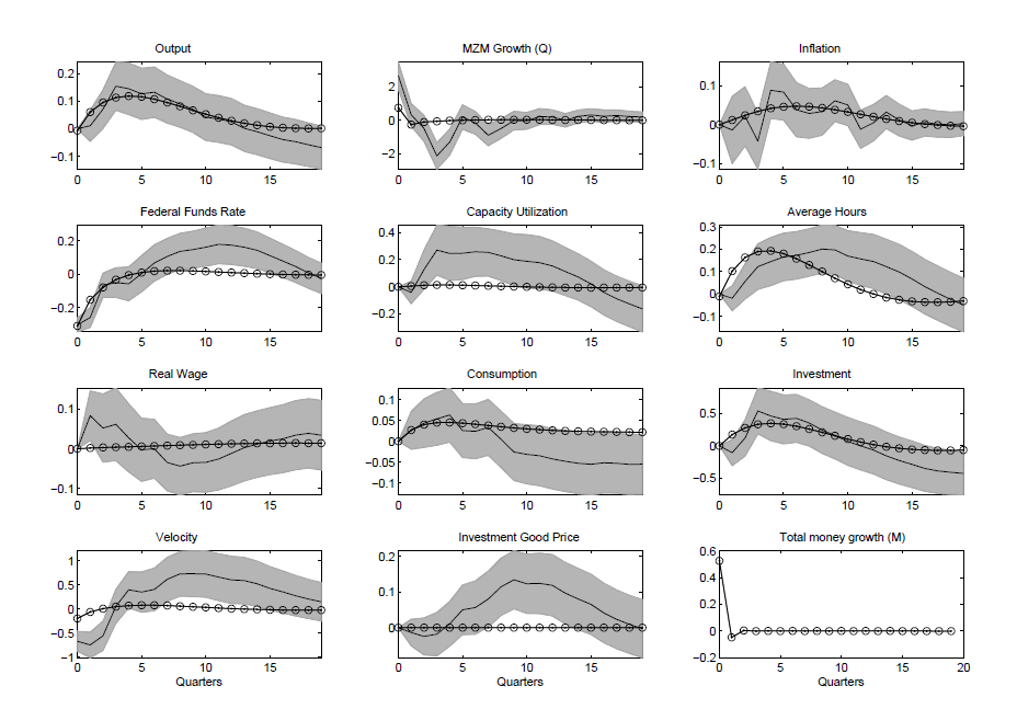
Data for Figure 1: Diagram (1,1) - Output
| x-axis | lower grey | solid line | line with o | upper grey |
|---|---|---|---|---|
| 0 | 6.73E-18 | 1.12E-16 | -0.00708 | 2.16E-16 |
| 1 | -0.04623 | 0.010777 | 0.060551 | 0.067787 |
| 2 | 0.000476 | 0.071111 | 0.095617 | 0.141746 |
| 3 | 0.066699 | 0.154647 | 0.113304 | 0.242594 |
| 4 | 0.051098 | 0.14547 | 0.118844 | 0.239843 |
| 5 | 0.033571 | 0.127066 | 0.11594 | 0.220561 |
| 6 | 0.040946 | 0.132773 | 0.107361 | 0.224599 |
| 7 | 0.020062 | 0.107769 | 0.095255 | 0.195477 |
| 8 | 0.004948 | 0.089997 | 0.081307 | 0.175047 |
| 9 | -0.01383 | 0.070347 | 0.066834 | 0.154524 |
| 10 | -0.04321 | 0.042128 | 0.052833 | 0.127471 |
| 11 | -0.04989 | 0.035428 | 0.040021 | 0.120747 |
| 12 | -0.05978 | 0.025119 | 0.02887 | 0.110015 |
| 13 | -0.0831 | 0.001311 | 0.019639 | 0.085718 |
| 14 | -0.09512 | -0.01091 | 0.012414 | 0.073294 |
| 15 | -0.10898 | -0.02564 | 0.007137 | 0.057698 |
| 16 | -0.12153 | -0.03942 | 0.003647 | 0.042684 |
| 17 | -0.1285 | -0.04739 | 0.001712 | 0.033729 |
| 18 | -0.13798 | -0.05838 | 0.001057 | 0.021209 |
| 19 | -0.14711 | -0.06854 | 0.001392 | 0.010028 |
Data for Figure 1: Diagram (1,2) - MZM Growth (Q)
| x-axis | lower grey | solid line | line with o | upper grey |
|---|---|---|---|---|
| 0 | 1.848742 | 2.678879 | 0.757207 | 3.509015 |
| 1 | -0.36591 | 0.327808 | -0.26236 | 1.021529 |
| 2 | -1.28066 | -0.49435 | -0.10592 | 0.291956 |
| 3 | -2.94588 | -2.14822 | -0.05958 | -1.35056 |
| 4 | -2.10708 | -1.31835 | -0.0232 | -0.52961 |
| 5 | -0.54422 | 0.194532 | 0.000617 | 0.933282 |
| 6 | -0.84926 | -0.16067 | 0.016096 | 0.527916 |
| 7 | -1.54711 | -0.90401 | 0.025398 | -0.2609 |
| 8 | -1.09403 | -0.49616 | 0.030078 | 0.101714 |
| 9 | -0.58945 | -0.02109 | 0.031304 | 0.547277 |
| 10 | -0.54701 | -0.03894 | 0.030007 | 0.469133 |
| 11 | -0.27007 | 0.220111 | 0.026961 | 0.71029 |
| 12 | -0.24765 | 0.192109 | 0.022816 | 0.631873 |
| 13 | -0.41434 | -0.00496 | 0.01811 | 0.404424 |
| 14 | -0.16295 | 0.228171 | 0.013277 | 0.619296 |
| 15 | -0.05731 | 0.319056 | 0.008653 | 0.69542 |
| 16 | -0.14058 | 0.243824 | 0.004483 | 0.628227 |
| 17 | -0.06115 | 0.286071 | 0.000926 | 0.633294 |
| 18 | -0.0967 | 0.225338 | -0.00193 | 0.547375 |
| 19 | -0.11839 | 0.192709 | -0.00407 | 0.50381 |
Data for Figure 1: Diagram (1,3) - Inflation
| x-axis | lower grey | solid line | line with o | upper grey |
|---|---|---|---|---|
| 0 | 1.28E-16 | 4.46E-16 | 0 | 7.64E-16 |
| 1 | -0.10033 | -0.01374 | 0.011922 | 0.072845 |
| 2 | -0.05437 | 0.021565 | 0.024017 | 0.0975 |
| 3 | -0.11404 | -0.04216 | 0.034287 | 0.029719 |
| 4 | 0.01578 | 0.088274 | 0.041755 | 0.160768 |
| 5 | 0.011592 | 0.083599 | 0.046125 | 0.155607 |
| 6 | -0.03139 | 0.038303 | 0.047528 | 0.107996 |
| 7 | -0.03505 | 0.028923 | 0.046346 | 0.092895 |
| 8 | -0.02712 | 0.033676 | 0.043098 | 0.094471 |
| 9 | 0.007607 | 0.061489 | 0.038353 | 0.11537 |
| 10 | -0.00245 | 0.050788 | 0.032669 | 0.104021 |
| 11 | -0.06096 | -0.01168 | 0.026557 | 0.037606 |
| 12 | -0.04196 | 0.005027 | 0.02045 | 0.052016 |
| 13 | -0.01011 | 0.032464 | 0.014697 | 0.075039 |
| 14 | -0.02918 | 0.011822 | 0.009552 | 0.052828 |
| 15 | -0.03979 | -0.00218 | 0.005182 | 0.035425 |
| 16 | -0.02933 | 0.005737 | 0.001673 | 0.040806 |
| 17 | -0.03215 | 0.001568 | -0.00096 | 0.03529 |
| 18 | -0.03294 | -9.2E-05 | -0.00275 | 0.032757 |
| 19 | -0.02825 | 0.002808 | -0.00378 | 0.033866 |
Data for Figure 1: Diagram (2, 1) - Federal Funds Rate
| x-axis | lower grey | solid line | line with o | upper grey |
|---|---|---|---|---|
| 0 | -0.34559 | -0.30307 | -0.30977 | -0.26055 |
| 1 | -0.31944 | -0.25963 | -0.15346 | -0.19983 |
| 2 | -0.13993 | -0.06654 | -0.07936 | 0.006841 |
| 3 | -0.13987 | -0.05058 | -0.03315 | 0.038706 |
| 4 | -0.1597 | -0.05816 | -0.00596 | 0.04337 |
| 5 | -0.10658 | 0.002295 | 0.009559 | 0.111168 |
| 6 | -0.04277 | 0.066247 | 0.017619 | 0.175267 |
| 7 | -0.00246 | 0.105783 | 0.020872 | 0.214027 |
| 8 | 0.027369 | 0.135785 | 0.021027 | 0.244202 |
| 9 | 0.035514 | 0.146178 | 0.019239 | 0.256842 |
| 10 | 0.046461 | 0.160947 | 0.016317 | 0.275432 |
| 11 | 0.061603 | 0.177654 | 0.012839 | 0.293705 |
| 12 | 0.057235 | 0.173218 | 0.009226 | 0.289201 |
| 13 | 0.046405 | 0.16075 | 0.005773 | 0.275096 |
| 14 | 0.032618 | 0.142305 | 0.002681 | 0.251993 |
| 15 | 0.006166 | 0.110607 | 7.42E-05 | 0.215047 |
| 16 | -0.02122 | 0.078558 | -0.00199 | 0.178339 |
| 17 | -0.05022 | 0.04536 | -0.0035 | 0.14094 |
| 18 | -0.085 | 0.007428 | -0.00448 | 0.099853 |
| 19 | -0.11587 | -0.02488 | -0.00498 | 0.066109 |
Data for Figure 1: Diagram (2,2) - Capacity Utilization
| x-axis | lower grey | solid line | line with o | upper grey |
|---|---|---|---|---|
| 0 | -6.2E-17 | 1.86E-17 | 0 | 9.88E-17 |
| 1 | -0.12495 | -0.0418 | 0.005158 | 0.04136 |
| 2 | -0.01874 | 0.126516 | 0.010927 | 0.271775 |
| 3 | 0.085111 | 0.269968 | 0.013245 | 0.454825 |
| 4 | 0.046916 | 0.245464 | 0.013279 | 0.444012 |
| 5 | 0.052388 | 0.246282 | 0.011878 | 0.440176 |
| 6 | 0.075704 | 0.257429 | 0.009641 | 0.439154 |
| 7 | 0.078493 | 0.253156 | 0.007001 | 0.42782 |
| 8 | 0.045675 | 0.227837 | 0.004273 | 0.409998 |
| 9 | 0.008089 | 0.198956 | 0.00168 | 0.389823 |
| 10 | -0.00955 | 0.187285 | -0.00063 | 0.384119 |
| 11 | -0.01633 | 0.177191 | -0.00255 | 0.370716 |
| 12 | -0.03218 | 0.153153 | -0.00406 | 0.338486 |
| 13 | -0.06485 | 0.112541 | -0.00513 | 0.289934 |
| 14 | -0.09862 | 0.072147 | -0.0058 | 0.242914 |
| 15 | -0.14679 | 0.021093 | -0.00611 | 0.188979 |
| 16 | -0.20774 | -0.04068 | -0.00611 | 0.126386 |
| 17 | -0.255 | -0.08787 | -0.00586 | 0.07925 |
| 18 | -0.29453 | -0.12631 | -0.00544 | 0.041906 |
| 19 | -0.33204 | -0.16217 | -0.0049 | 0.007699 |
Data for Figure 1: Diagram (2,3) - Average Hours
| x-axis | lower grey | solid line | line with o | upper grey |
|---|---|---|---|---|
| 0 | -1.2E-16 | -3.7E-17 | -0.01095 | 4.78E-17 |
| 1 | -0.07553 | -0.01932 | 0.102566 | 0.036895 |
| 2 | -0.02341 | 0.056135 | 0.163679 | 0.135679 |
| 3 | 0.020251 | 0.122582 | 0.190186 | 0.224914 |
| 4 | 0.036975 | 0.145182 | 0.193158 | 0.253389 |
| 5 | 0.058984 | 0.165992 | 0.180494 | 0.273 |
| 6 | 0.0663 | 0.172881 | 0.158009 | 0.279462 |
| 7 | 0.079359 | 0.185936 | 0.130105 | 0.292513 |
| 8 | 0.093098 | 0.201053 | 0.100134 | 0.309009 |
| 9 | 0.087488 | 0.197346 | 0.070604 | 0.307203 |
| 10 | 0.056311 | 0.170092 | 0.043319 | 0.283873 |
| 11 | 0.038719 | 0.15688 | 0.019483 | 0.275041 |
| 12 | 0.024063 | 0.145582 | -0.00021 | 0.267101 |
| 13 | -0.001 | 0.122261 | -0.01549 | 0.24552 |
| 14 | -0.02569 | 0.098292 | -0.02642 | 0.222272 |
| 15 | -0.05561 | 0.067562 | -0.03331 | 0.19073 |
| 16 | -0.08998 | 0.03255 | -0.03665 | 0.15508 |
| 17 | -0.11823 | 0.003811 | -0.03705 | 0.12585 |
| 18 | -0.14516 | -0.02414 | -0.03515 | 0.096886 |
| 19 | -0.16987 | -0.04943 | -0.03159 | 0.071006 |
Data for Figure 1: Diagram (3, 1) - Real Wage
| x-axis | lower grey | solid line | line with o | upper grey |
|---|---|---|---|---|
| 0 | -7.4E-17 | 3.72E-17 | 0 | 1.48E-16 |
| 1 | 0.020767 | 0.083568 | 0.001896 | 0.146369 |
| 2 | -0.03394 | 0.052215 | 0.003129 | 0.13837 |
| 3 | -0.0301 | 0.061799 | 0.004087 | 0.153701 |
| 4 | -0.05855 | 0.027656 | 0.004977 | 0.113863 |
| 5 | -0.08244 | -0.00256 | 0.005897 | 0.077311 |
| 6 | -0.07449 | 0.000195 | 0.006873 | 0.074876 |
| 7 | -0.10632 | -0.03465 | 0.007898 | 0.037021 |
| 8 | -0.11627 | -0.04391 | 0.008942 | 0.028454 |
| 9 | -0.1086 | -0.03531 | 0.009968 | 0.037979 |
| 10 | -0.1099 | -0.03441 | 0.010939 | 0.041077 |
| 11 | -0.10404 | -0.02587 | 0.011821 | 0.052296 |
| 12 | -0.09364 | -0.01162 | 0.012589 | 0.070409 |
| 13 | -0.08126 | 0.002664 | 0.013224 | 0.086592 |
| 14 | -0.07224 | 0.011825 | 0.013716 | 0.095894 |
| 15 | -0.0653 | 0.019414 | 0.014063 | 0.104126 |
| 16 | -0.06064 | 0.025278 | 0.014267 | 0.111193 |
| 17 | -0.05302 | 0.03439 | 0.014339 | 0.121802 |
| 18 | -0.04884 | 0.038897 | 0.014293 | 0.126636 |
| 19 | -0.05376 | 0.034257 | 0.014143 | 0.122273 |
Data for Figure 1: Diagram (3,2) - Consumption
| x-axis | lower grey | solid line | line with o | upper grey |
|---|---|---|---|---|
| 0 | -7.5E-17 | 3.72E-17 | 0 | 1.5E-16 |
| 1 | -0.01923 | 0.026329 | 0.026992 | 0.071891 |
| 2 | -0.01488 | 0.043457 | 0.039879 | 0.101794 |
| 3 | -0.00969 | 0.053834 | 0.044774 | 0.117358 |
| 4 | -0.00225 | 0.062925 | 0.045302 | 0.128099 |
| 5 | -0.03934 | 0.025643 | 0.043571 | 0.090629 |
| 6 | -0.04204 | 0.0238 | 0.040808 | 0.089637 |
| 7 | -0.03402 | 0.033326 | 0.037724 | 0.100672 |
| 8 | -0.06304 | 0.0048 | 0.034718 | 0.072644 |
| 9 | -0.09445 | -0.02577 | 0.032001 | 0.042904 |
| 10 | -0.10232 | -0.03135 | 0.029666 | 0.039628 |
| 11 | -0.10707 | -0.0347 | 0.027737 | 0.037669 |
| 12 | -0.11477 | -0.04227 | 0.026193 | 0.030226 |
| 13 | -0.12097 | -0.04803 | 0.024989 | 0.024908 |
| 14 | -0.12598 | -0.05273 | 0.024065 | 0.020529 |
| 15 | -0.12858 | -0.05525 | 0.023358 | 0.018081 |
| 16 | -0.12439 | -0.05166 | 0.022806 | 0.021065 |
| 17 | -0.12491 | -0.05284 | 0.022353 | 0.019239 |
| 18 | -0.1275 | -0.05545 | 0.021949 | 0.016599 |
| 19 | -0.12712 | -0.05507 | 0.021555 | 0.01698 |
Data for Figure 1: Diagram (3, 3) - Investment
| x-axis | lower grey | solid line | line with o | upper grey |
|---|---|---|---|---|
| 0 | 1.61E-16 | 3.9E-16 | 0 | 6.2E-16 |
| 1 | -0.30991 | -0.10552 | 0.174161 | 0.098875 |
| 2 | -0.16112 | 0.122519 | 0.279602 | 0.40616 |
| 3 | 0.184304 | 0.5422 | 0.333726 | 0.900095 |
| 4 | 0.079041 | 0.463475 | 0.34947 | 0.847909 |
| 5 | 0.029904 | 0.411013 | 0.337112 | 0.792122 |
| 6 | 0.054279 | 0.426393 | 0.305139 | 0.798506 |
| 7 | -0.00657 | 0.35438 | 0.260656 | 0.715329 |
| 8 | -0.11793 | 0.245109 | 0.209561 | 0.608145 |
| 9 | -0.20521 | 0.160255 | 0.156632 | 0.525725 |
| 10 | -0.30374 | 0.069054 | 0.105583 | 0.441852 |
| 11 | -0.37578 | -0.00121 | 0.05913 | 0.373366 |
| 12 | -0.43814 | -0.06526 | 0.01908 | 0.307618 |
| 13 | -0.52556 | -0.15508 | -0.01356 | 0.215405 |
| 14 | -0.59472 | -0.22786 | -0.03846 | 0.138997 |
| 15 | -0.64955 | -0.28705 | -0.05584 | 0.075459 |
| 16 | -0.70788 | -0.35033 | -0.06633 | 0.007227 |
| 17 | -0.73976 | -0.38861 | -0.07082 | -0.03746 |
| 18 | -0.75253 | -0.41111 | -0.07038 | -0.06968 |
| 19 | -0.76098 | -0.4282 | -0.06615 | -0.09542 |
Data for Figure 1: Diagram (4, 1) - Velocity
| x-axis | lower grey | solid line | line with o | upper grey |
|---|---|---|---|---|
| 0 | -0.87725 | -0.66972 | -0.19638 | -0.46219 |
| 1 | -1.01112 | -0.74433 | -0.06022 | -0.47754 |
| 2 | -0.85985 | -0.55502 | 0.007242 | -0.25018 |
| 3 | -0.29855 | 0.055033 | 0.048273 | 0.408618 |
| 4 | 0.019482 | 0.397513 | 0.069902 | 0.775543 |
| 5 | -0.06815 | 0.351375 | 0.07821 | 0.770903 |
| 6 | -0.03695 | 0.406826 | 0.07732 | 0.850603 |
| 7 | 0.158577 | 0.615054 | 0.070285 | 1.071531 |
| 8 | 0.265272 | 0.729741 | 0.059439 | 1.19421 |
| 9 | 0.25548 | 0.730734 | 0.046591 | 1.205989 |
| 10 | 0.241006 | 0.724947 | 0.033138 | 1.208889 |
| 11 | 0.172258 | 0.6603 | 0.02013 | 1.148341 |
| 12 | 0.112537 | 0.60322 | 0.008314 | 1.093902 |
| 13 | 0.104749 | 0.588768 | -0.00182 | 1.072787 |
| 14 | 0.050598 | 0.522456 | -0.01001 | 0.994315 |
| 15 | -0.02668 | 0.427421 | -0.01618 | 0.881518 |
| 16 | -0.0821 | 0.354114 | -0.02037 | 0.790327 |
| 17 | -0.14581 | 0.275027 | -0.02278 | 0.695862 |
| 18 | -0.20094 | 0.207672 | -0.02363 | 0.616284 |
| 19 | -0.25014 | 0.150037 | -0.02321 | 0.550208 |
Data for Figure 1: Diagram (4,2) - Investment Good Price
| x-axis | lower grey | solid line | line with o | upper grey |
|---|---|---|---|---|
| 0 | -1.7E-16 | -9.3E-17 | 0 | -1.8E-17 |
| 1 | -0.05103 | -0.01359 | 0 | 0.023851 |
| 2 | -0.07648 | -0.02451 | 0 | 0.027466 |
| 3 | -0.07906 | -0.01808 | 0 | 0.042906 |
| 4 | -0.0522 | 0.010664 | 0 | 0.073528 |
| 5 | -0.01972 | 0.049954 | 0 | 0.119625 |
| 6 | -0.01858 | 0.056261 | 0 | 0.131105 |
| 7 | 0.001604 | 0.080153 | 0 | 0.158702 |
| 8 | 0.033784 | 0.114304 | 0 | 0.194825 |
| 9 | 0.052727 | 0.134057 | 0 | 0.215387 |
| 10 | 0.039762 | 0.122885 | 0 | 0.206008 |
| 11 | 0.039027 | 0.123949 | 0 | 0.208872 |
| 12 | 0.032411 | 0.118499 | 0 | 0.204587 |
| 13 | 0.010089 | 0.096415 | 0 | 0.182741 |
| 14 | -0.00542 | 0.080421 | 0 | 0.166265 |
| 15 | -0.0195 | 0.065091 | 0 | 0.149686 |
| 16 | -0.04203 | 0.041388 | 0 | 0.124809 |
| 17 | -0.05901 | 0.023384 | 0 | 0.105775 |
| 18 | -0.07245 | 0.009179 | 0 | 0.090805 |
| 19 | -0.08414 | -0.00286 | 0 | 0.078424 |
Data for Figure 1: Diagram (4, 3) - Total Money Growth (M)
| x-axis | line with o |
|---|---|
| 0 | 0.52399 |
| 1 | -0.04814 |
| 2 | 0.004423 |
| 3 | -0.00041 |
| 4 | 3.73E-05 |
| 5 | -3.4E-06 |
| 6 | 3.15E-07 |
| 7 | -2.9E-08 |
| 8 | 2.66E-09 |
| 9 | -2.4E-10 |
| 10 | 2.24E-11 |
| 11 | -2.1E-12 |
| 12 | 1.89E-13 |
| 13 | -1.7E-14 |
| 14 | 1.6E-15 |
| 15 | -1.5E-16 |
| 16 | 1.35E-17 |
| 17 | -1.2E-18 |
| 18 | 1.14E-19 |
| 19 | -1E-20 |
Figure 2: Response to a neutral technology shock (o - Model, - VAR, grey area - 95% Confidence Interval)
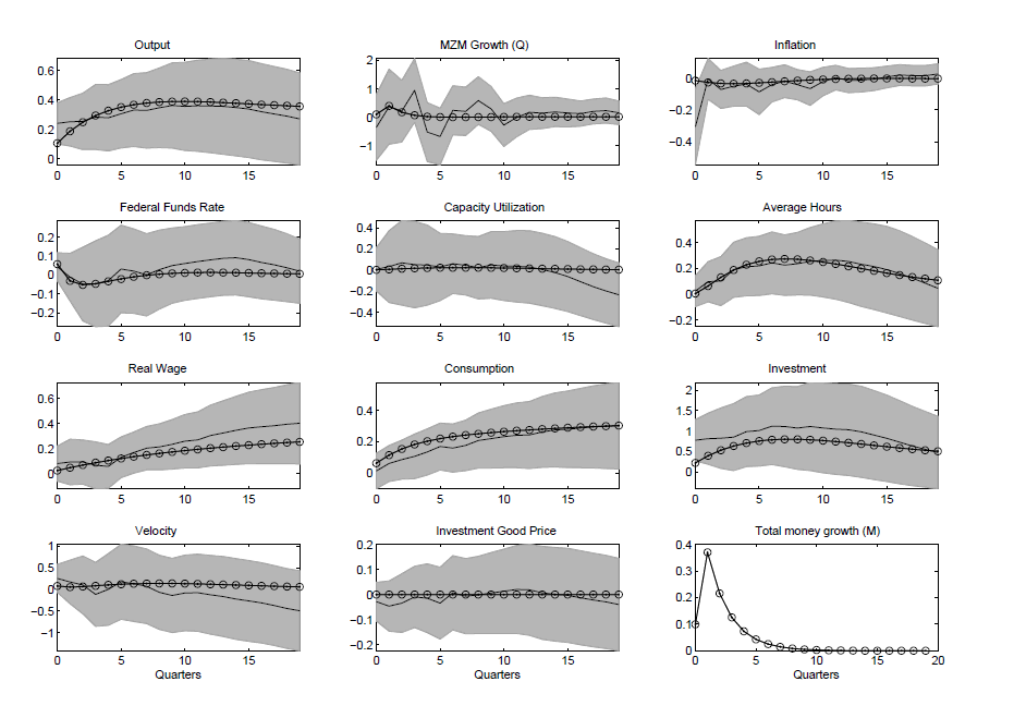
Data for Figure 2: Diagram(1,1) - Output
| x-axis: | lower grey | solid line | line with o | upper grey |
|---|---|---|---|---|
| 0 | 0.101268 | 0.240925 | 0.106552 | 0.380582 |
| 1 | 0.087057 | 0.251517 | 0.187688 | 0.415977 |
| 2 | 0.062784 | 0.254066 | 0.248385 | 0.445347 |
| 3 | 0.063419 | 0.283938 | 0.293376 | 0.504457 |
| 4 | 0.053774 | 0.278454 | 0.326393 | 0.503135 |
| 5 | 0.07427 | 0.306017 | 0.350237 | 0.537764 |
| 6 | 0.084006 | 0.330988 | 0.366976 | 0.57797 |
| 7 | 0.073179 | 0.328625 | 0.378155 | 0.584072 |
| 8 | 0.076166 | 0.346067 | 0.384959 | 0.615969 |
| 9 | 0.072768 | 0.361714 | 0.38833 | 0.650659 |
| 10 | 0.057023 | 0.355626 | 0.389044 | 0.654229 |
| 11 | 0.051317 | 0.359688 | 0.387755 | 0.668059 |
| 12 | 0.041431 | 0.358637 | 0.38502 | 0.675843 |
| 13 | 0.031148 | 0.355603 | 0.38131 | 0.680058 |
| 14 | 0.020518 | 0.34761 | 0.377022 | 0.674702 |
| 15 | 0.008799 | 0.337698 | 0.372476 | 0.666597 |
| 16 | -0.00622 | 0.319454 | 0.367924 | 0.64513 |
| 17 | -0.01731 | 0.304305 | 0.363554 | 0.625916 |
| 18 | -0.02807 | 0.289531 | 0.359492 | 0.607133 |
| 19 | -0.04 | 0.271194 | 0.355816 | 0.582385 |
Data for Figure 2: Diagram(1,2) - MZM Growth (Q)
| x-axis | lower grey | solid line | line with o | upper grey |
|---|---|---|---|---|
| 0 | -1.52235 | -0.35752 | 0.100351 | 0.807316 |
| 1 | -0.95485 | 0.371138 | 0.397225 | 1.697124 |
| 2 | -0.87418 | 0.21268 | 0.171893 | 1.299545 |
| 3 | -0.18091 | 0.944073 | 0.067095 | 2.069058 |
| 4 | -1.56449 | -0.52555 | 0.020687 | 0.513396 |
| 5 | -1.6789 | -0.6785 | 0.002523 | 0.321907 |
| 6 | -0.62727 | 0.240377 | -0.00222 | 1.108027 |
| 7 | -0.65081 | 0.204465 | -0.00093 | 1.059737 |
| 8 | -0.25553 | 0.585828 | 0.002713 | 1.427184 |
| 9 | -0.4999 | 0.290958 | 0.006858 | 1.081818 |
| 10 | -1.03509 | -0.27827 | 0.010613 | 0.478537 |
| 11 | -0.69013 | -0.00734 | 0.013584 | 0.67546 |
| 12 | -0.43279 | 0.171884 | 0.01564 | 0.776555 |
| 13 | -0.40269 | 0.140858 | 0.016798 | 0.684408 |
| 14 | -0.33449 | 0.18685 | 0.017152 | 0.708195 |
| 15 | -0.34357 | 0.147942 | 0.016832 | 0.63945 |
| 16 | -0.32187 | 0.125168 | 0.015987 | 0.572201 |
| 17 | -0.23744 | 0.202349 | 0.014765 | 0.642137 |
| 18 | -0.21396 | 0.232331 | 0.013302 | 0.678622 |
| 19 | -0.26106 | 0.155621 | 0.011721 | 0.572299 |
Data for Figure 2: Diagram(1,3) - Inflation
| x-axis | lower grey | solid line | line with o | upper grey |
|---|---|---|---|---|
| 0 | -0.5462 | -0.30648 | -0.01545 | -0.06676 |
| 1 | -0.1341 | -0.00509 | -0.02711 | 0.123926 |
| 2 | -0.19149 | -0.07156 | -0.03342 | 0.048373 |
| 3 | -0.17731 | -0.05079 | -0.03512 | 0.075736 |
| 4 | -0.17672 | -0.03793 | -0.03352 | 0.100868 |
| 5 | -0.23036 | -0.08679 | -0.02991 | 0.056783 |
| 6 | -0.15072 | -0.04157 | -0.02529 | 0.067588 |
| 7 | -0.12343 | -0.01958 | -0.02043 | 0.084277 |
| 8 | -0.13689 | -0.04141 | -0.01583 | 0.054074 |
| 9 | -0.17248 | -0.06634 | -0.01181 | 0.039802 |
| 10 | -0.11206 | -0.02189 | -0.00852 | 0.06828 |
| 11 | -0.07406 | 0.003435 | -0.00601 | 0.080927 |
| 12 | -0.09237 | -0.01565 | -0.00424 | 0.061074 |
| 13 | -0.08777 | -0.01249 | -0.00313 | 0.062784 |
| 14 | -0.07886 | -0.00639 | -0.00256 | 0.066089 |
| 15 | -0.06204 | 0.006875 | -0.0024 | 0.075792 |
| 16 | -0.04725 | 0.019096 | -0.00253 | 0.085443 |
| 17 | -0.04946 | 0.015466 | -0.00282 | 0.080394 |
| 18 | -0.05011 | 0.014753 | -0.00317 | 0.07962 |
| 19 | -0.03773 | 0.026299 | -0.0035 | 0.090329 |
Data for Figure 2: Diagram(2,1) - Federal Funds Rate
| x-axis | lower grey | solid line | line with o | upper grey |
|---|---|---|---|---|
| 0 | -0.03107 | 0.043869 | 0.058264 | 0.118808 |
| 1 | -0.13801 | -0.01104 | -0.03111 | 0.115926 |
| 2 | -0.24374 | -0.04774 | -0.0516 | 0.148266 |
| 3 | -0.27461 | -0.04611 | -0.04644 | 0.182391 |
| 4 | -0.27099 | -0.02956 | -0.03376 | 0.211862 |
| 5 | -0.20118 | 0.032151 | -0.02069 | 0.265477 |
| 6 | -0.20378 | 0.020866 | -0.00966 | 0.245514 |
| 7 | -0.21781 | 0.001164 | -0.00118 | 0.220136 |
| 8 | -0.18097 | 0.028911 | 0.004923 | 0.238795 |
| 9 | -0.15002 | 0.05 | 0.009051 | 0.250018 |
| 10 | -0.13464 | 0.061371 | 0.011601 | 0.257381 |
| 11 | -0.12476 | 0.071623 | 0.012929 | 0.268011 |
| 12 | -0.11577 | 0.080378 | 0.013334 | 0.27653 |
| 13 | -0.10778 | 0.088785 | 0.013061 | 0.285349 |
| 14 | -0.10638 | 0.091963 | 0.012312 | 0.290311 |
| 15 | -0.11562 | 0.082021 | 0.011251 | 0.279663 |
| 16 | -0.12653 | 0.067224 | 0.010013 | 0.26098 |
| 17 | -0.1339 | 0.054564 | 0.008705 | 0.243024 |
| 18 | -0.14199 | 0.038665 | 0.007409 | 0.219324 |
| 19 | -0.15053 | 0.020613 | 0.006186 | 0.191752 |
Data for Figure 2: Diagram(2,2) - Capacity Utilization
| x-axis | lower grey | solid line | line with o | upper grey |
|---|---|---|---|---|
| 0 | -0.1975 | 0.007209 | 0.003238 | 0.211918 |
| 1 | -0.30517 | 0.033948 | 0.007359 | 0.373069 |
| 2 | -0.33033 | 0.069275 | 0.012851 | 0.468876 |
| 3 | -0.35516 | 0.052617 | 0.017527 | 0.460396 |
| 4 | -0.33011 | 0.047843 | 0.020819 | 0.425794 |
| 5 | -0.28807 | 0.029863 | 0.022751 | 0.347799 |
| 6 | -0.2205 | 0.060723 | 0.023534 | 0.341948 |
| 7 | -0.23443 | 0.045358 | 0.023412 | 0.325145 |
| 8 | -0.27163 | 0.023343 | 0.022609 | 0.318313 |
| 9 | -0.26583 | 0.048762 | 0.021319 | 0.363349 |
| 10 | -0.28701 | 0.038863 | 0.019703 | 0.364736 |
| 11 | -0.30125 | 0.036383 | 0.017892 | 0.374017 |
| 12 | -0.31221 | 0.03026 | 0.015995 | 0.372729 |
| 13 | -0.336 | 0.006249 | 0.014095 | 0.348497 |
| 14 | -0.36127 | -0.02223 | 0.012257 | 0.316807 |
| 15 | -0.39039 | -0.0598 | 0.01053 | 0.270797 |
| 16 | -0.42862 | -0.10842 | 0.008946 | 0.21179 |
| 17 | -0.46626 | -0.15558 | 0.007522 | 0.155112 |
| 18 | -0.49993 | -0.19603 | 0.006266 | 0.10788 |
| 19 | -0.53342 | -0.2321 | 0.005177 | 0.069216 |
Data for Figure 2: Diagram(2,3) - Average Hours
| x-axis | lower grey | solid line | line with o | upper grey |
|---|---|---|---|---|
| 0 | -0.0982 | 0.023049 | 0.003455 | 0.144297 |
| 1 | -0.06036 | 0.09631 | 0.062703 | 0.252978 |
| 2 | -0.09016 | 0.10101 | 0.130271 | 0.292181 |
| 3 | -0.02617 | 0.188984 | 0.186823 | 0.404142 |
| 4 | -0.01419 | 0.211871 | 0.227974 | 0.437934 |
| 5 | -0.01125 | 0.219274 | 0.254552 | 0.449802 |
| 6 | 0.001815 | 0.242692 | 0.268869 | 0.483568 |
| 7 | -0.01113 | 0.224861 | 0.273391 | 0.460849 |
| 8 | -0.0075 | 0.235948 | 0.270337 | 0.479392 |
| 9 | -0.00868 | 0.254483 | 0.261607 | 0.517645 |
| 10 | -0.0234 | 0.261429 | 0.248803 | 0.546261 |
| 11 | -0.04084 | 0.263886 | 0.233273 | 0.568608 |
| 12 | -0.06631 | 0.25323 | 0.216137 | 0.572765 |
| 13 | -0.09657 | 0.231477 | 0.198316 | 0.559522 |
| 14 | -0.12128 | 0.212618 | 0.180548 | 0.546516 |
| 15 | -0.14693 | 0.190183 | 0.163398 | 0.527295 |
| 16 | -0.17497 | 0.15896 | 0.147281 | 0.492892 |
| 17 | -0.2021 | 0.123097 | 0.132471 | 0.448296 |
| 18 | -0.22862 | 0.085004 | 0.11912 | 0.398625 |
| 19 | -0.25415 | 0.045239 | 0.107281 | 0.344626 |
Data for Figure 2: Diagram(3,1) - Real Wage
| x-axis | lower grey | solid line | line with o | upper grey |
|---|---|---|---|---|
| 0 | -0.06092 | 0.079995 | 0.024403 | 0.220913 |
| 1 | -0.08987 | 0.093016 | 0.047325 | 0.275901 |
| 2 | -0.08458 | 0.092563 | 0.068275 | 0.26971 |
| 3 | -0.12138 | 0.066773 | 0.087305 | 0.254929 |
| 4 | -0.11823 | 0.057689 | 0.104633 | 0.233607 |
| 5 | -0.03315 | 0.130383 | 0.120494 | 0.293919 |
| 6 | 0.00325 | 0.168325 | 0.135097 | 0.3334 |
| 7 | 0.029143 | 0.203369 | 0.148608 | 0.377596 |
| 8 | 0.029222 | 0.213949 | 0.161158 | 0.398675 |
| 9 | 0.035213 | 0.234214 | 0.172847 | 0.433215 |
| 10 | 0.04511 | 0.259354 | 0.183751 | 0.473598 |
| 11 | 0.044642 | 0.269577 | 0.193929 | 0.494512 |
| 12 | 0.060632 | 0.304439 | 0.203427 | 0.548246 |
| 13 | 0.066229 | 0.324782 | 0.212282 | 0.583335 |
| 14 | 0.073267 | 0.34578 | 0.220527 | 0.618292 |
| 15 | 0.07835 | 0.365314 | 0.228189 | 0.652278 |
| 16 | 0.077405 | 0.374879 | 0.235295 | 0.672352 |
| 17 | 0.076896 | 0.382969 | 0.24187 | 0.689043 |
| 18 | 0.078173 | 0.394972 | 0.247938 | 0.71177 |
| 19 | 0.076138 | 0.4031 | 0.253525 | 0.730061 |
Data for Figure 2: Diagram(3,2) - Consumption
| x-axis | lower grey | solid line | line with o | upper grey |
|---|---|---|---|---|
| 0 | -0.09751 | 0.015196 | 0.0645 | 0.127902 |
| 1 | -0.0522 | 0.062523 | 0.115866 | 0.177246 |
| 2 | -0.03739 | 0.086866 | 0.154553 | 0.211124 |
| 3 | -0.03381 | 0.107949 | 0.183136 | 0.249709 |
| 4 | -0.0107 | 0.135994 | 0.204317 | 0.282692 |
| 5 | 0.020843 | 0.170052 | 0.220303 | 0.319262 |
| 6 | 0.007101 | 0.160088 | 0.23272 | 0.313074 |
| 7 | 0.016596 | 0.177238 | 0.242702 | 0.33788 |
| 8 | 0.033018 | 0.208243 | 0.251013 | 0.383469 |
| 9 | 0.033702 | 0.22026 | 0.258159 | 0.406818 |
| 10 | 0.035472 | 0.232655 | 0.264469 | 0.429838 |
| 11 | 0.035595 | 0.241488 | 0.270157 | 0.447382 |
| 12 | 0.030577 | 0.243303 | 0.275359 | 0.456029 |
| 13 | 0.037708 | 0.262614 | 0.280164 | 0.487519 |
| 14 | 0.039568 | 0.274945 | 0.284625 | 0.510321 |
| 15 | 0.036561 | 0.279782 | 0.288777 | 0.523002 |
| 16 | 0.035515 | 0.287254 | 0.29264 | 0.538993 |
| 17 | 0.033728 | 0.294387 | 0.296226 | 0.555045 |
| 18 | 0.03012 | 0.298299 | 0.29954 | 0.566478 |
| 19 | 0.026901 | 0.30184 | 0.302586 | 0.576779 |
Data for Figure 2: Diagram(3,3) - Investment
| x-axis | lower grey | solid line | line with o | upper grey |
|---|---|---|---|---|
| 0 | 0.268189 | 0.775782 | 0.216858 | 1.283376 |
| 1 | 0.183256 | 0.811995 | 0.39336 | 1.440734 |
| 2 | 0.081392 | 0.825198 | 0.530383 | 1.569003 |
| 3 | 0.027621 | 0.852072 | 0.6329 | 1.676524 |
| 4 | 0.124318 | 0.986427 | 0.706399 | 1.848536 |
| 5 | 0.139611 | 1.013396 | 0.75578 | 1.887181 |
| 6 | 0.177043 | 1.120618 | 0.78519 | 2.064193 |
| 7 | 0.123543 | 1.113251 | 0.798151 | 2.102958 |
| 8 | 0.056859 | 1.074604 | 0.79772 | 2.092349 |
| 9 | 0.028348 | 1.111692 | 0.786616 | 2.195036 |
| 10 | -0.02668 | 1.076269 | 0.767288 | 2.179212 |
| 11 | -0.06569 | 1.046148 | 0.741944 | 2.157987 |
| 12 | -0.09202 | 1.032106 | 0.71255 | 2.156229 |
| 13 | -0.13937 | 0.980859 | 0.680824 | 2.101089 |
| 14 | -0.19107 | 0.902205 | 0.648223 | 1.995481 |
| 15 | -0.23971 | 0.822467 | 0.615938 | 1.884646 |
| 16 | -0.29586 | 0.726945 | 0.584897 | 1.749753 |
| 17 | -0.34146 | 0.633662 | 0.555777 | 1.608786 |
| 18 | -0.37747 | 0.553351 | 0.529026 | 1.484174 |
| 19 | -0.41562 | 0.4734 | 0.504888 | 1.362416 |
Data for Figure 2: Diagram(4,1) - Velocity
| x-axis | lower grey | solid line | line with o | upper grey |
|---|---|---|---|---|
| 0 | -0.07049 | 0.253684 | 0.077658 | 0.577855 |
| 1 | -0.33574 | 0.17022 | 0.052808 | 0.676178 |
| 2 | -0.56835 | 0.101708 | 0.062297 | 0.771765 |
| 3 | -0.85834 | -0.11713 | 0.08186 | 0.624071 |
| 4 | -0.83189 | -0.00071 | 0.101445 | 0.830465 |
| 5 | -0.69322 | 0.174776 | 0.117288 | 1.042771 |
| 6 | -0.74629 | 0.129262 | 0.128352 | 1.004816 |
| 7 | -0.79374 | 0.070888 | 0.13473 | 0.935512 |
| 8 | -0.92781 | -0.06848 | 0.136955 | 0.79085 |
| 9 | -1.00135 | -0.14216 | 0.135702 | 0.717041 |
| 10 | -0.96052 | -0.08415 | 0.131664 | 0.792221 |
| 11 | -0.97083 | -0.07739 | 0.125499 | 0.816045 |
| 12 | -1.03751 | -0.12533 | 0.117809 | 0.786854 |
| 13 | -1.09378 | -0.1667 | 0.109128 | 0.760384 |
| 14 | -1.15833 | -0.223 | 0.099921 | 0.712327 |
| 15 | -1.20432 | -0.26818 | 0.090575 | 0.667959 |
| 16 | -1.24426 | -0.31294 | 0.081403 | 0.618374 |
| 17 | -1.30137 | -0.37481 | 0.072647 | 0.551751 |
| 18 | -1.36967 | -0.44398 | 0.06448 | 0.481716 |
| 19 | -1.42002 | -0.49465 | 0.057011 | 0.430722 |
Data for Figure 2: Diagram(4,2) - Investment Good Price
| x-axis | lower grey | solid line | line with o | upper grey |
|---|---|---|---|---|
| 0 | -0.10642 | -0.02848 | 0 | 0.049461 |
| 1 | -0.14675 | -0.04607 | 0 | 0.054613 |
| 2 | -0.1518 | -0.03422 | 0 | 0.083358 |
| 3 | -0.13195 | -0.00931 | 0 | 0.113332 |
| 4 | -0.15267 | -0.01468 | 0 | 0.123303 |
| 5 | -0.17824 | -0.03433 | 0 | 0.109585 |
| 6 | -0.14148 | 0.007226 | 0 | 0.15593 |
| 7 | -0.15686 | -0.0063 | 0 | 0.144268 |
| 8 | -0.15591 | -0.00131 | 0 | 0.153297 |
| 9 | -0.15562 | 0.006305 | 0 | 0.168231 |
| 10 | -0.15541 | 0.013352 | 0 | 0.182114 |
| 11 | -0.15556 | 0.020582 | 0 | 0.196725 |
| 12 | -0.16326 | 0.018969 | 0 | 0.201195 |
| 13 | -0.17929 | 0.006905 | 0 | 0.193095 |
| 14 | -0.18638 | 0.001169 | 0 | 0.188719 |
| 15 | -0.19171 | -0.00329 | 0 | 0.185137 |
| 16 | -0.20115 | -0.01275 | 0 | 0.17565 |
| 17 | -0.20925 | -0.02162 | 0 | 0.166022 |
| 18 | -0.21594 | -0.02936 | 0 | 0.157229 |
| 19 | -0.22445 | -0.03965 | 0 | 0.145157 |
Data for Figure 2: Diagram(4,3) - Total money growth (M)
| x-axis | line with o |
|---|---|
| 0 | 0.099144 |
| 1 | 0.369489 |
| 2 | 0.215345 |
| 3 | 0.125507 |
| 4 | 0.073148 |
| 5 | 0.042632 |
| 6 | 0.024847 |
| 7 | 0.014481 |
| 8 | 0.00844 |
| 9 | 0.004919 |
| 10 | 0.002867 |
| 11 | 0.001671 |
| 12 | 0.000974 |
| 13 | 0.000568 |
| 14 | 0.000331 |
| 15 | 0.000193 |
| 16 | 0.000112 |
| 17 | 6.55E-05 |
| 18 | 3.82E-05 |
| 19 | 2.22E-05 |
Figure 3: Response to an embodied technology shock (o - Model, - VAR, grey area - 95% Confidence Interval)
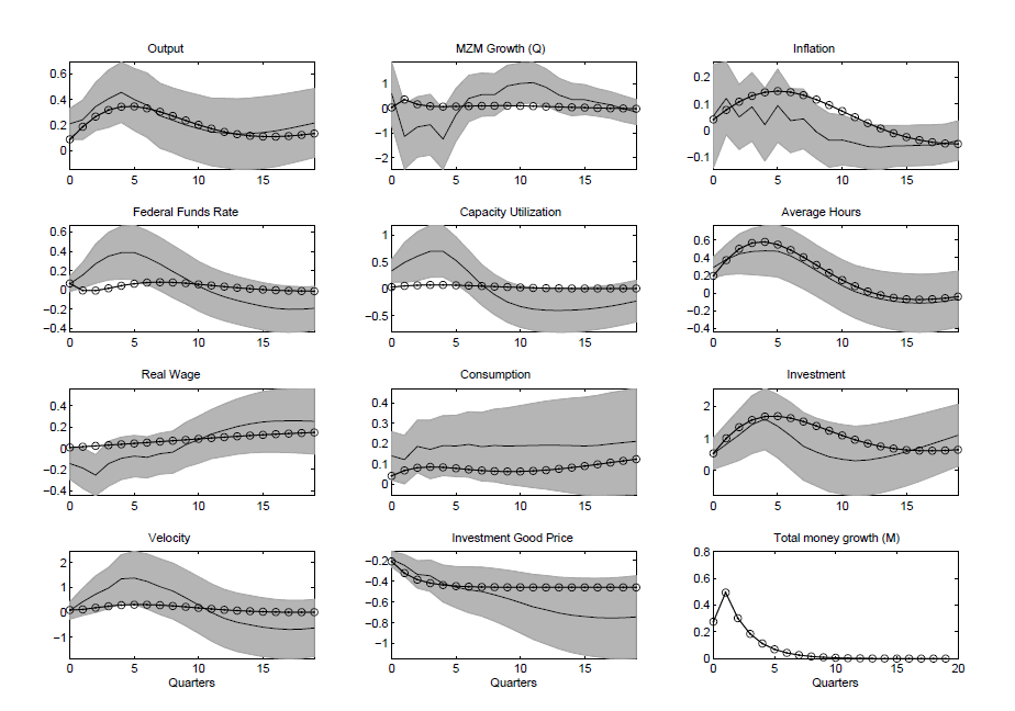
Data for Figure 3: Diagram(1,1) - Output
| x-axis | lower grey | solid line | line with o | upper grey |
|---|---|---|---|---|
| 0 | 0.088211 | 0.209443 | 0.088604 | 0.330674 |
| 1 | 0.086692 | 0.24125 | 0.186215 | 0.395807 |
| 2 | 0.156014 | 0.343893 | 0.26535 | 0.531773 |
| 3 | 0.181425 | 0.405355 | 0.317386 | 0.629285 |
| 4 | 0.219433 | 0.455104 | 0.342548 | 0.690774 |
| 5 | 0.157045 | 0.399203 | 0.344973 | 0.64136 |
| 6 | 0.103346 | 0.35524 | 0.330182 | 0.607134 |
| 7 | 0.019717 | 0.273187 | 0.303808 | 0.526657 |
| 8 | -0.01528 | 0.237363 | 0.270961 | 0.490002 |
| 9 | -0.05895 | 0.200686 | 0.235938 | 0.460326 |
| 10 | -0.08812 | 0.173626 | 0.202125 | 0.43537 |
| 11 | -0.11788 | 0.146215 | 0.171997 | 0.410313 |
| 12 | -0.13265 | 0.138021 | 0.14718 | 0.408695 |
| 13 | -0.14512 | 0.130119 | 0.128561 | 0.405362 |
| 14 | -0.14372 | 0.133516 | 0.116403 | 0.410752 |
| 15 | -0.13804 | 0.142006 | 0.110477 | 0.422054 |
| 16 | -0.12441 | 0.154562 | 0.11019 | 0.433531 |
| 17 | -0.10248 | 0.173643 | 0.114705 | 0.449767 |
| 18 | -0.0785 | 0.194615 | 0.123048 | 0.467729 |
| 19 | -0.05262 | 0.216208 | 0.134202 | 0.485033 |
Data for Figure 3: Diagram(1,2) - MZM Growth (Q)
| x-axis | lower grey | solid line | line with o | upper grey |
|---|---|---|---|---|
| 0 | -0.68441 | 0.598721 | 0.038139 | 1.881856 |
| 1 | -2.47321 | -1.14332 | 0.36074 | 0.186562 |
| 2 | -1.99322 | -0.76045 | 0.161081 | 0.472325 |
| 3 | -1.90408 | -0.66563 | 0.085297 | 0.572832 |
| 4 | -2.4839 | -1.25493 | 0.068427 | -0.02595 |
| 5 | -1.34769 | -0.26667 | 0.075826 | 0.81435 |
| 6 | -0.54556 | 0.402888 | 0.089599 | 1.351334 |
| 7 | -0.32125 | 0.558306 | 0.101118 | 1.437863 |
| 8 | -0.30605 | 0.553149 | 0.106852 | 1.41235 |
| 9 | 0.064795 | 0.912553 | 0.106031 | 1.760311 |
| 10 | 0.17257 | 1.010905 | 0.099313 | 1.84924 |
| 11 | 0.226143 | 1.045611 | 0.088018 | 1.865079 |
| 12 | 0.102093 | 0.856862 | 0.073686 | 1.61163 |
| 13 | -0.14816 | 0.541376 | 0.057815 | 1.230908 |
| 14 | -0.3019 | 0.360285 | 0.041723 | 1.022473 |
| 15 | -0.25716 | 0.353748 | 0.026475 | 0.964656 |
| 16 | -0.32282 | 0.23992 | 0.01286 | 0.802659 |
| 17 | -0.40228 | 0.140406 | 0.001395 | 0.683094 |
| 18 | -0.54443 | -0.01279 | -0.00765 | 0.51885 |
| 19 | -0.65856 | -0.14897 | -0.01422 | 0.360625 |
Data for Figure 3: Diagram(1,3) - Inflation
| x-axis | lower grey | solid line | line with o | upper grey |
|---|---|---|---|---|
| 0 | -0.1428 | 0.053425 | 0.040297 | 0.24965 |
| 1 | -0.01739 | 0.120011 | 0.076709 | 0.257417 |
| 2 | -0.07318 | 0.049769 | 0.107221 | 0.172721 |
| 3 | -0.04153 | 0.088368 | 0.129868 | 0.218264 |
| 4 | -0.11711 | 0.020833 | 0.143508 | 0.158776 |
| 5 | -0.04538 | 0.093022 | 0.147972 | 0.231425 |
| 6 | -0.0851 | 0.036169 | 0.143926 | 0.157436 |
| 7 | -0.07025 | 0.042861 | 0.132644 | 0.155973 |
| 8 | -0.10757 | -0.00649 | 0.115762 | 0.094593 |
| 9 | -0.14034 | -0.03821 | 0.095061 | 0.063924 |
| 10 | -0.13213 | -0.03725 | 0.072293 | 0.057631 |
| 11 | -0.13729 | -0.04882 | 0.049051 | 0.039646 |
| 12 | -0.14591 | -0.06186 | 0.026683 | 0.022182 |
| 13 | -0.14812 | -0.06461 | 0.006249 | 0.018894 |
| 14 | -0.1381 | -0.05981 | -0.0115 | 0.018487 |
| 15 | -0.13604 | -0.05893 | -0.02609 | 0.018177 |
| 16 | -0.1345 | -0.05706 | -0.03735 | 0.020368 |
| 17 | -0.13238 | -0.05594 | -0.04529 | 0.020494 |
| 18 | -0.12406 | -0.05037 | -0.05014 | 0.023324 |
| 19 | -0.11391 | -0.03929 | -0.05223 | 0.035323 |
Data for Figure 3: Diagram(2,1) - Federal Funds Rate
| x-axis | lower grey | solid line | line with o | upper grey |
|---|---|---|---|---|
| 0 | -0.01741 | 0.063132 | 0.065738 | 0.143674 |
| 1 | 0.020907 | 0.153481 | -0.0079 | 0.286055 |
| 2 | 0.066666 | 0.27012 | -0.00851 | 0.473574 |
| 3 | 0.101414 | 0.349607 | 0.015491 | 0.5978 |
| 4 | 0.111476 | 0.385577 | 0.042201 | 0.659678 |
| 5 | 0.104196 | 0.387221 | 0.062848 | 0.670245 |
| 6 | 0.053925 | 0.334798 | 0.074943 | 0.61567 |
| 7 | -0.00957 | 0.267958 | 0.078849 | 0.545488 |
| 8 | -0.08243 | 0.189998 | 0.076078 | 0.462425 |
| 9 | -0.14804 | 0.115859 | 0.068468 | 0.379762 |
| 10 | -0.21982 | 0.037428 | 0.057791 | 0.29468 |
| 11 | -0.27822 | -0.0244 | 0.045588 | 0.229414 |
| 12 | -0.32305 | -0.07232 | 0.033104 | 0.178414 |
| 13 | -0.35805 | -0.10999 | 0.021282 | 0.138065 |
| 14 | -0.3894 | -0.14201 | 0.010779 | 0.105377 |
| 15 | -0.41802 | -0.17139 | 0.002001 | 0.075237 |
| 16 | -0.43662 | -0.19269 | -0.00486 | 0.051236 |
| 17 | -0.44187 | -0.2019 | -0.00977 | 0.038077 |
| 18 | -0.43533 | -0.20126 | -0.01286 | 0.032815 |
| 19 | -0.41751 | -0.19152 | -0.01431 | 0.034478 |
Data for Figure 3: Diagram(2,2) - Capacity Utilization
| x-axis | lower grey | solid line | line with o | upper grey |
|---|---|---|---|---|
| 0 | 0.123679 | 0.336123 | 0.032831 | 0.548567 |
| 1 | 0.118328 | 0.492531 | 0.053123 | 0.866735 |
| 2 | 0.149173 | 0.608503 | 0.065878 | 1.067834 |
| 3 | 0.213433 | 0.701057 | 0.071541 | 1.188681 |
| 4 | 0.217923 | 0.701157 | 0.071425 | 1.184392 |
| 5 | 0.090057 | 0.53103 | 0.067068 | 0.972003 |
| 6 | -0.08717 | 0.315387 | 0.059939 | 0.717948 |
| 7 | -0.30575 | 0.074222 | 0.051309 | 0.45419 |
| 8 | -0.48487 | -0.10783 | 0.042204 | 0.269205 |
| 9 | -0.63007 | -0.24788 | 0.033401 | 0.134304 |
| 10 | -0.72101 | -0.33068 | 0.025448 | 0.059656 |
| 11 | -0.7798 | -0.37948 | 0.018688 | 0.020847 |
| 12 | -0.80625 | -0.3995 | 0.013296 | 0.007242 |
| 13 | -0.8144 | -0.40403 | 0.009306 | 0.006338 |
| 14 | -0.81081 | -0.39992 | 0.006649 | 0.010956 |
| 15 | -0.78937 | -0.38193 | 0.005182 | 0.025512 |
| 16 | -0.76128 | -0.35846 | 0.004713 | 0.044359 |
| 17 | -0.72301 | -0.32541 | 0.005028 | 0.072191 |
| 18 | -0.67475 | -0.28141 | 0.00591 | 0.111929 |
| 19 | -0.61984 | -0.22992 | 0.00715 | 0.160005 |
Data for Figure 3: Diagram(2,3) - Average Hours
| x-axis | lower grey | solid line | line with o | upper grey |
|---|---|---|---|---|
| 0 | 0.173053 | 0.291596 | 0.195479 | 0.410139 |
| 1 | 0.208716 | 0.379333 | 0.372974 | 0.549951 |
| 2 | 0.217455 | 0.443747 | 0.500449 | 0.67004 |
| 3 | 0.208175 | 0.470485 | 0.567881 | 0.732796 |
| 4 | 0.196931 | 0.479446 | 0.58042 | 0.761962 |
| 5 | 0.181025 | 0.474683 | 0.54933 | 0.768342 |
| 6 | 0.119035 | 0.421284 | 0.487438 | 0.723532 |
| 7 | 0.047495 | 0.344083 | 0.406915 | 0.640672 |
| 8 | -0.03592 | 0.25482 | 0.318253 | 0.545561 |
| 9 | -0.12187 | 0.168465 | 0.229871 | 0.458804 |
| 10 | -0.2085 | 0.085169 | 0.148054 | 0.378838 |
| 11 | -0.28343 | 0.016421 | 0.077083 | 0.316268 |
| 12 | -0.34034 | -0.03099 | 0.019462 | 0.278352 |
| 13 | -0.38489 | -0.06751 | -0.0238 | 0.249864 |
| 14 | -0.41469 | -0.09221 | -0.05291 | 0.230274 |
| 15 | -0.43648 | -0.10833 | -0.06894 | 0.21983 |
| 16 | -0.4445 | -0.1148 | -0.07361 | 0.214902 |
| 17 | -0.4362 | -0.10882 | -0.069 | 0.21856 |
| 18 | -0.41462 | -0.09136 | -0.05734 | 0.231898 |
| 19 | -0.38427 | -0.0674 | -0.04082 | 0.249469 |
Data for Figure 3: Diagram(3,1) - Real Wage
| x-axis | lower grey | solid line | line with o | upper grey |
|---|---|---|---|---|
| 0 | -0.29258 | -0.14483 | 0.007573 | 0.00292 |
| 1 | -0.37978 | -0.18706 | 0.014977 | 0.005663 |
| 2 | -0.44574 | -0.25351 | 0.022264 | -0.06128 |
| 3 | -0.3588 | -0.14574 | 0.029639 | 0.06732 |
| 4 | -0.29629 | -0.09511 | 0.037274 | 0.106071 |
| 5 | -0.26977 | -0.07407 | 0.045256 | 0.121635 |
| 6 | -0.27995 | -0.08585 | 0.053584 | 0.10826 |
| 7 | -0.2448 | -0.05138 | 0.062185 | 0.142034 |
| 8 | -0.23592 | -0.03645 | 0.070947 | 0.163015 |
| 9 | -0.1771 | 0.033685 | 0.079733 | 0.244473 |
| 10 | -0.14271 | 0.080527 | 0.088411 | 0.303765 |
| 11 | -0.09847 | 0.134026 | 0.096859 | 0.366525 |
| 12 | -0.07784 | 0.170326 | 0.104977 | 0.418494 |
| 13 | -0.05612 | 0.205279 | 0.11269 | 0.466681 |
| 14 | -0.0444 | 0.229853 | 0.119953 | 0.504105 |
| 15 | -0.0387 | 0.248301 | 0.126743 | 0.535303 |
| 16 | -0.03826 | 0.257375 | 0.133062 | 0.553014 |
| 17 | -0.04178 | 0.258769 | 0.138928 | 0.559322 |
| 18 | -0.04737 | 0.25866 | 0.144376 | 0.564692 |
| 19 | -0.05558 | 0.254841 | 0.149447 | 0.565262 |
Data for Figure 3: Diagram(3,2) - Consumption
| x-axis | lower grey | solid line | line with o | upper grey |
|---|---|---|---|---|
| 0 | 0.018699 | 0.13835 | 0.039777 | 0.258001 |
| 1 | 5.78E-05 | 0.119776 | 0.066061 | 0.239494 |
| 2 | 0.055616 | 0.185212 | 0.079537 | 0.314807 |
| 3 | 0.025296 | 0.170408 | 0.083523 | 0.315519 |
| 4 | 0.040544 | 0.188961 | 0.081588 | 0.337378 |
| 5 | 0.035573 | 0.186903 | 0.076698 | 0.338234 |
| 6 | 0.032796 | 0.194721 | 0.071022 | 0.356646 |
| 7 | 0.014309 | 0.183701 | 0.066001 | 0.353094 |
| 8 | 0.010004 | 0.189532 | 0.062494 | 0.369059 |
| 9 | -0.00257 | 0.186412 | 0.060926 | 0.375392 |
| 10 | -0.00978 | 0.188503 | 0.061415 | 0.38679 |
| 11 | -0.01931 | 0.189363 | 0.063875 | 0.398035 |
| 12 | -0.02593 | 0.19156 | 0.068092 | 0.409052 |
| 13 | -0.03602 | 0.190237 | 0.073781 | 0.416499 |
| 14 | -0.04566 | 0.188975 | 0.080626 | 0.423607 |
| 15 | -0.05426 | 0.187229 | 0.088311 | 0.428721 |
| 16 | -0.05713 | 0.190077 | 0.096538 | 0.437285 |
| 17 | -0.05561 | 0.197367 | 0.105043 | 0.45034 |
| 18 | -0.0537 | 0.203582 | 0.1136 | 0.460864 |
| 19 | -0.05127 | 0.210038 | 0.122027 | 0.471343 |
Data for Figure 3: Diagram(3,3) - Investment
| x-axis | lower grey | solid line | line with o | upper grey |
|---|---|---|---|---|
| 0 | 0.03997 | 0.529258 | 0.535965 | 1.018545 |
| 1 | 0.173285 | 0.819248 | 1.00464 | 1.465211 |
| 2 | 0.317051 | 1.11317 | 1.354948 | 1.909289 |
| 3 | 0.526471 | 1.431237 | 1.577948 | 2.336003 |
| 4 | 0.648917 | 1.606976 | 1.685211 | 2.565034 |
| 5 | 0.391813 | 1.383717 | 1.697299 | 2.37562 |
| 6 | 0.042616 | 1.086801 | 1.637557 | 2.130986 |
| 7 | -0.30294 | 0.756053 | 1.528765 | 1.815046 |
| 8 | -0.48442 | 0.57632 | 1.391355 | 1.63706 |
| 9 | -0.66172 | 0.42758 | 1.242536 | 1.516883 |
| 10 | -0.73602 | 0.35133 | 1.095952 | 1.438683 |
| 11 | -0.77811 | 0.303781 | 0.961703 | 1.385674 |
| 12 | -0.76035 | 0.328904 | 0.846576 | 1.418155 |
| 13 | -0.69806 | 0.393457 | 0.754426 | 1.484974 |
| 14 | -0.59778 | 0.482321 | 0.686639 | 1.562419 |
| 15 | -0.47798 | 0.590159 | 0.642632 | 1.658294 |
| 16 | -0.34071 | 0.708258 | 0.620353 | 1.757224 |
| 17 | -0.18582 | 0.834974 | 0.616753 | 1.855769 |
| 18 | -0.02477 | 0.968336 | 0.62821 | 1.961438 |
| 19 | 0.132043 | 1.101587 | 0.650888 | 2.07113 |
Data for Figure 3: Diagram(4,1) - Velocity
| x-axis | lower grey | solid line | line with o | upper grey |
|---|---|---|---|---|
| 0 | -0.27578 | 0.073119 | 0.088999 | 0.422016 |
| 1 | -0.13095 | 0.420759 | 0.115328 | 0.972473 |
| 2 | -0.01451 | 0.725958 | 0.180616 | 1.466428 |
| 3 | 0.145405 | 0.975918 | 0.24333 | 1.80643 |
| 4 | 0.368582 | 1.344606 | 0.28675 | 2.32063 |
| 5 | 0.305222 | 1.378627 | 0.306682 | 2.452033 |
| 6 | 0.130375 | 1.242985 | 0.304959 | 2.355595 |
| 7 | -0.09273 | 1.032071 | 0.285992 | 2.15687 |
| 8 | -0.27357 | 0.856337 | 0.254958 | 1.986241 |
| 9 | -0.54927 | 0.58197 | 0.216853 | 1.713207 |
| 10 | -0.84969 | 0.292871 | 0.176027 | 1.435436 |
| 11 | -1.16177 | -0.00815 | 0.135981 | 1.145475 |
| 12 | -1.41396 | -0.24602 | 0.099319 | 0.921909 |
| 13 | -1.58506 | -0.40542 | 0.067786 | 0.774211 |
| 14 | -1.69299 | -0.50705 | 0.042364 | 0.678895 |
| 15 | -1.78815 | -0.60173 | 0.023389 | 0.584689 |
| 16 | -1.84425 | -0.66342 | 0.010684 | 0.517409 |
| 17 | -1.86736 | -0.69343 | 0.003689 | 0.480505 |
| 18 | -1.84769 | -0.68185 | 0.00159 | 0.483991 |
| 19 | -1.78851 | -0.63284 | 0.003427 | 0.522834 |
Data for Figure 3: Diagram(4,2) - Investment Good Price
| x-axis | lower grey | solid line | line with o | upper grey |
|---|---|---|---|---|
| 0 | -0.26296 | -0.18668 | -0.20746 | -0.11039 |
| 1 | -0.35038 | -0.24515 | -0.32104 | -0.13992 |
| 2 | -0.46621 | -0.33321 | -0.38322 | -0.2002 |
| 3 | -0.49897 | -0.34633 | -0.41726 | -0.19369 |
| 4 | -0.60093 | -0.42126 | -0.43589 | -0.24159 |
| 5 | -0.65645 | -0.45645 | -0.4461 | -0.25646 |
| 6 | -0.70495 | -0.48199 | -0.45168 | -0.25904 |
| 7 | -0.73706 | -0.49934 | -0.45474 | -0.26163 |
| 8 | -0.78646 | -0.53063 | -0.45641 | -0.27481 |
| 9 | -0.84071 | -0.5659 | -0.45733 | -0.29109 |
| 10 | -0.90031 | -0.60539 | -0.45783 | -0.31046 |
| 11 | -0.9614 | -0.64639 | -0.45811 | -0.33138 |
| 12 | -1.00833 | -0.67593 | -0.45826 | -0.34353 |
| 13 | -1.05417 | -0.70619 | -0.45834 | -0.3582 |
| 14 | -1.0891 | -0.72733 | -0.45838 | -0.36555 |
| 15 | -1.11422 | -0.74121 | -0.45841 | -0.3682 |
| 16 | -1.13319 | -0.75107 | -0.45842 | -0.36895 |
| 17 | -1.14528 | -0.75573 | -0.45843 | -0.36619 |
| 18 | -1.14767 | -0.7525 | -0.45843 | -0.35732 |
| 19 | -1.14332 | -0.74432 | -0.45844 | -0.34533 |
Data for Figure 3: Diagram(4,3) - Total money growth (M)
| x-axis | line with o |
|---|---|
| 0 | 0.275081 |
| 1 | 0.493062 |
| 2 | 0.301902 |
| 3 | 0.184855 |
| 4 | 0.113186 |
| 5 | 0.069304 |
| 6 | 0.042435 |
| 7 | 0.025983 |
| 8 | 0.015909 |
| 9 | 0.009741 |
| 10 | 0.005965 |
| 11 | 0.003652 |
| 12 | 0.002236 |
| 13 | 0.001369 |
| 14 | 0.000838 |
| 15 | 0.000513 |
| 16 | 0.000314 |
| 17 | 0.000192 |
| 18 | 0.000118 |
| 19 | 7.22E-05 |
Figure 4a: Quasi First Difference of Change in Inflation versus Log, Marginal Cost
Data for Figure 4a
| Scatter Plot: s_t_hata | Scatter Plot: y_a | Red Line: x | Red Line: 0.013556*x | Black Line: x | Black Line: 0.676*x |
|---|---|---|---|---|---|
| 0.029208 | -0.00154 | -0.05 | -0.0006778 | -0.05 | -33.8 |
| 0.034452 | 0.005042 | -0.049 | -0.0006642 | -0.049 | -33.124 |
| 0.046509 | -0.0031 | -0.048 | -0.0006507 | -0.048 | -32.448 |
| 0.041289 | -0.00349 | -0.047 | -0.0006371 | -0.047 | -31.772 |
| 0.039133 | 0.00535 | -0.046 | -0.0006236 | -0.046 | -31.096 |
| 0.031474 | -0.00087 | -0.045 | -0.00061 | -0.045 | -30.42 |
| 0.026714 | -0.00149 | -0.044 | -0.0005965 | -0.044 | -29.744 |
| 0.016661 | -0.00403 | -0.043 | -0.0005829 | -0.043 | -29.068 |
| 0.011772 | 0.005695 | -0.042 | -0.0005694 | -0.042 | -28.392 |
| 0.01342 | -0.00754 | -0.041 | -0.0005558 | -0.041 | -27.716 |
| 0.013138 | 0.008689 | -0.04 | -0.0005422 | -0.04 | -27.04 |
| 0.010459 | -0.00321 | -0.039 | -0.0005287 | -0.039 | -26.364 |
| 0.01105 | 0.001033 | -0.038 | -0.0005151 | -0.038 | -25.688 |
| 0.010752 | -0.00651 | -0.037 | -0.0005016 | -0.037 | -25.012 |
| 0.010889 | 0.010344 | -0.036 | -0.000488 | -0.036 | -24.336 |
| 0.011018 | -0.00395 | -0.035 | -0.0004745 | -0.035 | -23.66 |
| 0.008013 | -0.00387 | -0.034 | -0.0004609 | -0.034 | -22.984 |
| 0.015986 | 0.00363 | -0.033 | -0.0004473 | -0.033 | -22.308 |
| 0.013353 | -0.00132 | -0.032 | -0.0004338 | -0.032 | -21.632 |
| 0.010317 | -0.00061 | -0.031 | -0.0004202 | -0.031 | -20.956 |
| 0.009784 | -0.00014 | -0.03 | -0.0004067 | -0.03 | -20.28 |
| 0.02228 | -0.00093 | -0.029 | -0.0003931 | -0.029 | -19.604 |
| 0.020944 | 0.004456 | -0.028 | -0.0003796 | -0.028 | -18.928 |
| 0.019823 | -0.00473 | -0.027 | -0.000366 | -0.027 | -18.252 |
| 0.020486 | 0.002148 | -0.026 | -0.0003525 | -0.026 | -17.576 |
| 0.018531 | -0.00139 | -0.025 | -0.0003389 | -0.025 | -16.9 |
| 0.021817 | 0.000175 | -0.024 | -0.0003253 | -0.024 | -16.224 |
| 0.025108 | -0.00052 | -0.023 | -0.0003118 | -0.023 | -15.548 |
| 0.022728 | 0.005183 | -0.022 | -0.0002982 | -0.022 | -14.872 |
| 0.01923 | -0.00737 | -0.021 | -0.0002847 | -0.021 | -14.196 |
| 0.01091 | 0.005477 | -0.02 | -0.0002711 | -0.02 | -13.52 |
| 0.001427 | 0.000759 | -0.019 | -0.0002576 | -0.019 | -12.844 |
| -0.00237 | -0.00233 | -0.018 | -0.000244 | -0.018 | -12.168 |
| 0.001309 | -0.00512 | -0.017 | -0.0002305 | -0.017 | -11.492 |
| -0.00082 | 0.005327 | -0.016 | -0.0002169 | -0.016 | -10.816 |
| 0.001005 | 0.002415 | -0.015 | -0.0002033 | -0.015 | -10.14 |
| 0.000579 | -0.00145 | -0.014 | -0.0001898 | -0.014 | -9.464 |
| 0.004278 | -0.00559 | -0.013 | -0.0001762 | -0.013 | -8.788 |
| -0.00473 | 0.009631 | -0.012 | -0.0001627 | -0.012 | -8.112 |
| -0.00544 | -0.00601 | -0.011 | -0.0001491 | -0.011 | -7.436 |
| -0.00779 | 0.002447 | -0.01 | -0.0001356 | -0.01 | -6.76 |
| -0.0082 | -0.00257 | -0.009 | -0.000122 | -0.009 | -6.084 |
| -0.01048 | 0.001314 | -0.008 | -0.0001084 | -0.008 | -5.408 |
| -0.01372 | 0.000389 | -0.007 | -9.49E-05 | -0.007 | -4.732 |
| -0.01124 | -0.00161 | -0.006 | -8.13E-05 | -0.006 | -4.056 |
| -0.01677 | -0.00188 | -0.005 | -6.78E-05 | -0.005 | -3.38 |
| -0.01539 | 0.004814 | -0.004 | -5.42E-05 | -0.004 | -2.704 |
| -0.01056 | -0.00106 | -0.003 | -4.07E-05 | -0.003 | -2.028 |
| -0.01113 | -0.00219 | -0.002 | -2.71E-05 | -0.002 | -1.352 |
| -0.01797 | 0.000222 | -0.001 | -1.36E-05 | -0.001 | -0.676 |
| -0.01887 | 0.002604 | 0 | 0 | 0 | 0 |
| -0.02138 | -0.00399 | 0.001 | 1.36E-05 | 0.001 | 0.676 |
| -0.02204 | 0.003846 | 0.002 | 2.71E-05 | 0.002 | 1.352 |
| -0.02672 | -0.00335 | 0.003 | 4.07E-05 | 0.003 | 2.028 |
| -0.02131 | 0.004365 | 0.004 | 5.42E-05 | 0.004 | 2.704 |
| -0.02044 | -0.00378 | 0.005 | 6.78E-05 | 0.005 | 3.38 |
| -0.01678 | 0.000934 | 0.006 | 8.13E-05 | 0.006 | 4.056 |
| -0.01892 | -0.00144 | 0.007 | 9.49E-05 | 0.007 | 4.732 |
| -0.02393 | 0.0044 | 0.008 | 0.00010845 | 0.008 | 5.408 |
| -0.026 | -0.0024 | 0.009 | 0.000122 | 0.009 | 6.084 |
| -0.02225 | -0.00261 | 0.01 | 0.00013556 | 0.01 | 6.76 |
| -0.02275 | 0.001115 | 0.011 | 0.00014912 | 0.011 | 7.436 |
| -0.01957 | 0.005813 | 0.012 | 0.00016267 | 0.012 | 8.112 |
| -0.02294 | -0.00659 | 0.013 | 0.00017623 | 0.013 | 8.788 |
| -0.02334 | 0.002021 | 0.014 | 0.00018978 | 0.014 | 9.464 |
| -0.01185 | 0.000517 | 0.015 | 0.00020334 | 0.015 | 10.14 |
| -0.00097 | 0.000157 | 0.016 | 0.0002169 | 0.016 | 10.816 |
| 0.008702 | -0.00283 | 0.017 | 0.00023045 | 0.017 | 11.492 |
| 0.011584 | 0.002165 | 0.018 | 0.00024401 | 0.018 | 12.168 |
| 0.011939 | -0.00081 | 0.019 | 0.00025756 | 0.019 | 12.844 |
| 0.018053 | 0.001132 | 0.02 | 0.00027112 | 0.02 | 13.52 |
| 0.017166 | -0.00044 | 0.021 | 0.00028468 | 0.021 | 14.196 |
| 0.017432 | -0.00086 | 0.022 | 0.00029823 | 0.022 | 14.872 |
| 0.018884 | -0.00386 | 0.023 | 0.00031179 | 0.023 | 15.548 |
| 0.04619 | 0.009287 | 0.024 | 0.00032534 | 0.024 | 16.224 |
| 0.029381 | -0.00547 | 0.025 | 0.0003389 | 0.025 | 16.9 |
| 0.04479 | 0.001919 | 0.026 | 0.00035246 | 0.026 | 17.576 |
| 0.037178 | -0.00504 | 0.027 | 0.00036601 | 0.027 | 18.252 |
| 0.045086 | 0.004416 | 0.028 | 0.00037957 | 0.028 | 18.928 |
| 0.029681 | 0.002994 | 0.029 | 0.00039312 | 0.029 | 19.604 |
| 0.022669 | -0.00433 | 0.03 | 0.00040668 | 0.03 | 20.28 |
| 0.009324 | 0.002243 | 0.031 | 0.00042024 | 0.031 | 20.956 |
| 0.005911 | -0.00129 | 0.032 | 0.00043379 | 0.032 | 21.632 |
| 0.009254 | -0.00027 | 0.033 | 0.00044735 | 0.033 | 22.308 |
| 0.001693 | -0.00158 | 0.034 | 0.0004609 | 0.034 | 22.984 |
| -0.0033 | -0.00044 | 0.035 | 0.00047446 | 0.035 | 23.66 |
| -0.00605 | 0.006769 | 0.036 | 0.00048802 | 0.036 | 24.336 |
| -0.00469 | -0.00651 | 0.037 | 0.00050157 | 0.037 | 25.012 |
| -0.01327 | 0.001693 | 0.038 | 0.00051513 | 0.038 | 25.688 |
| -0.01187 | -0.00343 | 0.039 | 0.00052868 | 0.039 | 26.364 |
| -0.02445 | 0.003628 | 0.04 | 0.00054224 | 0.04 | 27.04 |
| -0.02896 | 0.003691 | 0.041 | 0.0005558 | 0.041 | 27.716 |
| -0.02329 | -0.00595 | 0.042 | 0.00056935 | 0.042 | 28.392 |
| -0.01953 | 0.000476 | 0.043 | 0.00058291 | 0.043 | 29.068 |
| -0.02872 | 0.006503 | 0.044 | 0.00059646 | 0.044 | 29.744 |
| -0.02907 | -0.00938 | 0.045 | 0.00061002 | 0.045 | 30.42 |
| -0.03095 | 0.005421 | 0.046 | 0.00062358 | 0.046 | 31.096 |
| -0.02835 | -0.00015 | 0.047 | 0.00063713 | 0.047 | 31.772 |
| -0.02788 | 0.001462 | 0.048 | 0.00065069 | 0.048 | 32.448 |
| -0.03688 | -0.00201 | 0.049 | 0.00066424 | 0.049 | 33.124 |
| -0.03486 | 0.001456 | 0.05 | 0.0006778 | 0.05 | 33.8 |
| -0.01852 | -0.00644 | ||||
| -0.01911 | 0.010386 | ||||
| -0.02973 | -0.00423 | ||||
| -0.0379 | -0.00359 | ||||
| -0.03454 | 0.002299 | ||||
| -0.03785 | 0.003283 | ||||
| -0.04762 | -0.00951 |
Figure 4b: Projection of Quasi First Difference of the Change in Inflation versus Projection of Log, Marginal Cost
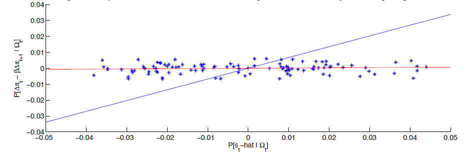
Data for Figure 4b
| Scatter Plot: s_t_hat_b | Scatter Plot: y_b | Red Line: x | Red Line: 0.0136*x | Black Line: x | Black Line: 0.676*x |
|---|---|---|---|---|---|
| 0.0312381 | -0.003819526 | -0.05 | -0.00068 | -0.05 | -0.0338 |
| 0.0440444 | 0.000741893 | -0.049 | -0.00066 | -0.049 | -0.03312 |
| 0.0403026 | 0.00474885 | -0.048 | -0.00065 | -0.048 | -0.03245 |
| 0.0361257 | -0.003267628 | -0.047 | -0.00064 | -0.047 | -0.03177 |
| 0.0298339 | -0.001862649 | -0.046 | -0.00062 | -0.046 | -0.0311 |
| 0.0256114 | 0.001754228 | -0.045 | -0.00061 | -0.045 | -0.03042 |
| 0.0167275 | 0.004309099 | -0.044 | -0.0006 | -0.044 | -0.02974 |
| 0.0097462 | -0.00346506 | -0.043 | -0.00058 | -0.043 | -0.02907 |
| 0.0134596 | 0.004285389 | -0.042 | -0.00057 | -0.042 | -0.02839 |
| 0.0104026 | -0.004478456 | -0.041 | -0.00056 | -0.041 | -0.02772 |
| 0.0096338 | -0.001288309 | -0.04 | -0.00054 | -0.04 | -0.02704 |
| 0.0098113 | 0.000570151 | -0.039 | -0.00053 | -0.039 | -0.02636 |
| 0.0110049 | 0.005536147 | -0.038 | -0.00052 | -0.038 | -0.02569 |
| 0.0077785 | -0.006524401 | -0.037 | -0.0005 | -0.037 | -0.02501 |
| 0.0101223 | -0.001353794 | -0.036 | -0.00049 | -0.036 | -0.02434 |
| 0.008174 | 0.005435381 | -0.035 | -0.00047 | -0.035 | -0.02366 |
| 0.0137231 | -0.001393737 | -0.034 | -0.00046 | -0.034 | -0.02298 |
| 0.0123032 | -0.000589309 | -0.033 | -0.00045 | -0.033 | -0.02231 |
| 0.0095164 | 0.001128872 | -0.032 | -0.00043 | -0.032 | -0.02163 |
| 0.0087452 | 0.00038016 | -0.031 | -0.00042 | -0.031 | -0.02096 |
| 0.020417 | 0.001141303 | -0.03 | -0.00041 | -0.03 | -0.02028 |
| 0.0185566 | -0.00372499 | -0.029 | -0.00039 | -0.029 | -0.0196 |
| 0.0192108 | 0.002242038 | -0.028 | -0.00038 | -0.028 | -0.01893 |
| 0.0187694 | 0.000303036 | -0.027 | -0.00037 | -0.027 | -0.01825 |
| 0.0173814 | 0.000219488 | -0.026 | -0.00035 | -0.026 | -0.01758 |
| 0.0201902 | 0.000569998 | -0.025 | -0.00034 | -0.025 | -0.0169 |
| 0.0234371 | 0.000477538 | -0.024 | -0.00033 | -0.024 | -0.01622 |
| 0.0201391 | -0.004608136 | -0.023 | -0.00031 | -0.023 | -0.01555 |
| 0.0192884 | 0.004306912 | -0.022 | -0.0003 | -0.022 | -0.01487 |
| 0.0093039 | -0.001704815 | -0.021 | -0.00028 | -0.021 | -0.0142 |
| 0.0004919 | -0.003575111 | -0.02 | -0.00027 | -0.02 | -0.01352 |
| -0.002456 | 0.001671427 | -0.019 | -0.00026 | -0.019 | -0.01284 |
| 0.0015925 | 0.005905414 | -0.018 | -0.00024 | -0.018 | -0.01217 |
| -0.002396 | -0.002592393 | -0.017 | -0.00023 | -0.017 | -0.01149 |
| -0.000763 | -0.004865536 | -0.016 | -0.00022 | -0.016 | -0.01082 |
| -4.09E-05 | 0.000109434 | -0.015 | -0.0002 | -0.015 | -0.01014 |
| 0.004515 | 0.005925398 | -0.014 | -0.00019 | -0.014 | -0.00946 |
| -0.00682 | -0.006505205 | -0.013 | -0.00018 | -0.013 | -0.00879 |
| -0.00525 | 0.000849609 | -0.012 | -0.00016 | -0.012 | -0.00811 |
| -0.008428 | 0.000497887 | -0.011 | -0.00015 | -0.011 | -0.00744 |
| -0.008275 | 0.001112453 | -0.01 | -0.00014 | -0.01 | -0.00676 |
| -0.010977 | -0.000120303 | -0.009 | -0.00012 | -0.009 | -0.00608 |
| -0.01409 | -0.001165638 | -0.008 | -0.00011 | -0.008 | -0.00541 |
| -0.011435 | 0.001251908 | -0.007 | -9.49E-05 | -0.007 | -0.00473 |
| -0.016261 | 0.002325331 | -0.006 | -8.13E-05 | -0.006 | -0.00406 |
| -0.016708 | -0.00367529 | -0.005 | -6.78E-05 | -0.005 | -0.00338 |
| -0.011265 | -0.00136965 | -0.004 | -5.42E-05 | -0.004 | -0.0027 |
| -0.010987 | 0.002439215 | -0.003 | -4.07E-05 | -0.003 | -0.00203 |
| -0.017806 | 0.000612908 | -0.002 | -2.71E-05 | -0.002 | -0.00135 |
| -0.019606 | -0.002682645 | -0.001 | -1.36E-05 | -0.001 | -0.00068 |
| -0.020618 | 0.002282399 | 0 | 0 | 0 | 0 |
| -0.022706 | -0.001808079 | 0.001 | 1.36E-05 | 0.001 | 0.000676 |
| -0.02591 | 0.001024213 | 0.002 | 2.71E-05 | 0.002 | 0.001352 |
| -0.022423 | -0.002503506 | 0.003 | 4.07E-05 | 0.003 | 0.002028 |
| -0.020009 | 0.001293288 | 0.004 | 5.42E-05 | 0.004 | 0.002704 |
| -0.017173 | 0.00089523 | 0.005 | 6.78E-05 | 0.005 | 0.00338 |
| -0.018737 | 0.000721175 | 0.006 | 8.13E-05 | 0.006 | 0.004056 |
| -0.024623 | -0.003639043 | 0.007 | 9.49E-05 | 0.007 | 0.004732 |
| -0.025566 | -7.85E-05 | 0.008 | 0.000108 | 0.008 | 0.005408 |
| -0.021748 | 0.003514437 | 0.009 | 0.000122 | 0.009 | 0.006084 |
| -0.022869 | 7.05E-05 | 0.01 | 0.000136 | 0.01 | 0.00676 |
| -0.021223 | -0.006044145 | 0.011 | 0.000149 | 0.011 | 0.007436 |
| -0.021695 | 0.003130946 | 0.012 | 0.000163 | 0.012 | 0.008112 |
| -0.023419 | 0.00115082 | 0.013 | 0.000176 | 0.013 | 0.008788 |
| -0.01298 | -0.001381497 | 0.014 | 0.00019 | 0.014 | 0.009464 |
| -0.002267 | -0.000290402 | 0.015 | 0.000203 | 0.015 | 0.01014 |
| 0.007822 | 0.002684492 | 0.016 | 0.000217 | 0.016 | 0.010816 |
| 0.0099533 | -0.000628824 | 0.017 | 0.00023 | 0.017 | 0.011492 |
| 0.0107789 | -0.000312299 | 0.018 | 0.000244 | 0.018 | 0.012168 |
| 0.0161816 | -0.000569191 | 0.019 | 0.000258 | 0.019 | 0.012844 |
| 0.0158629 | -0.000159201 | 0.02 | 0.000271 | 0.02 | 0.01352 |
| 0.0162574 | 0.001012083 | 0.021 | 0.000285 | 0.021 | 0.014196 |
| 0.0183073 | 0.004033951 | 0.022 | 0.000298 | 0.022 | 0.014872 |
| 0.040823 | -0.006261543 | 0.023 | 0.000312 | 0.023 | 0.015548 |
| 0.0290046 | 0.000368508 | 0.024 | 0.000325 | 0.024 | 0.016224 |
| 0.0417282 | 0.001195147 | 0.025 | 0.000339 | 0.025 | 0.0169 |
| 0.0364844 | 0.003711597 | 0.026 | 0.000352 | 0.026 | 0.017576 |
| 0.0417502 | -0.001461173 | 0.027 | 0.000366 | 0.027 | 0.018252 |
| 0.0276205 | -0.005145002 | 0.028 | 0.00038 | 0.028 | 0.018928 |
| 0.0222098 | 0.002487935 | 0.029 | 0.000393 | 0.029 | 0.019604 |
| 0.0085341 | -0.000246265 | 0.03 | 0.000407 | 0.03 | 0.02028 |
| 0.0052158 | 1.37E-05 | 0.031 | 0.00042 | 0.031 | 0.020956 |
| 0.0081361 | 0.000892407 | 0.032 | 0.000434 | 0.032 | 0.021632 |
| 0.0015289 | 0.001420979 | 0.033 | 0.000447 | 0.033 | 0.022308 |
| -0.003584 | 0.001016476 | 0.034 | 0.000461 | 0.034 | 0.022984 |
| -0.008024 | -0.006233572 | 0.035 | 0.000474 | 0.035 | 0.02366 |
| -0.004327 | 0.00273558 | 0.036 | 0.000488 | 0.036 | 0.024336 |
| -0.01326 | 0.001321564 | 0.037 | 0.000502 | 0.037 | 0.025012 |
| -0.01167 | 0.002292398 | 0.038 | 0.000515 | 0.038 | 0.025688 |
| -0.024517 | -0.002079079 | 0.039 | 0.000529 | 0.039 | 0.026364 |
| -0.029644 | -0.005437949 | 0.04 | 0.000542 | 0.04 | 0.02704 |
| -0.022445 | 0.003704349 | 0.041 | 0.000556 | 0.041 | 0.027716 |
| -0.019601 | 0.002361313 | 0.042 | 0.000569 | 0.042 | 0.028392 |
| -0.029663 | -0.006610842 | 0.043 | 0.000583 | 0.043 | 0.029068 |
| -0.027164 | 0.00543157 | 0.044 | 0.000596 | 0.044 | 0.029744 |
| -0.031307 | -0.000717032 | 0.045 | 0.00061 | 0.045 | 0.03042 |
| -0.028605 | -0.002604243 | 0.046 | 0.000624 | 0.046 | 0.031096 |
| -0.028095 | -0.001445105 | 0.047 | 0.000637 | 0.047 | 0.031772 |
| -0.035703 | 0.000823834 | 0.048 | 0.000651 | 0.048 | 0.032448 |
| -0.034798 | -0.000540383 | 0.049 | 0.000664 | 0.049 | 0.033124 |
| -0.018048 | 0.005439342 | 0.05 | 0.000678 | 0.05 | 0.0338 |
| -0.021208 | -0.006710305 | ||||
| -0.028752 | -0.001425232 | ||||
| -0.036041 | 0.005064872 | ||||
| -0.034647 | -0.000538518 | ||||
| -0.038128 | -0.004426075 |
Figure 5: Firm-Specific Capital and the Response of Price to Marginal Cost Shocks
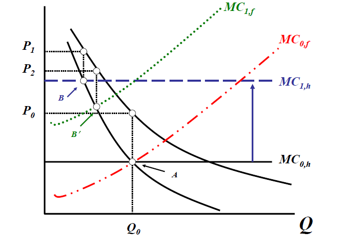
Figure 6: Features of Distribution of Output and Prices Across Firms
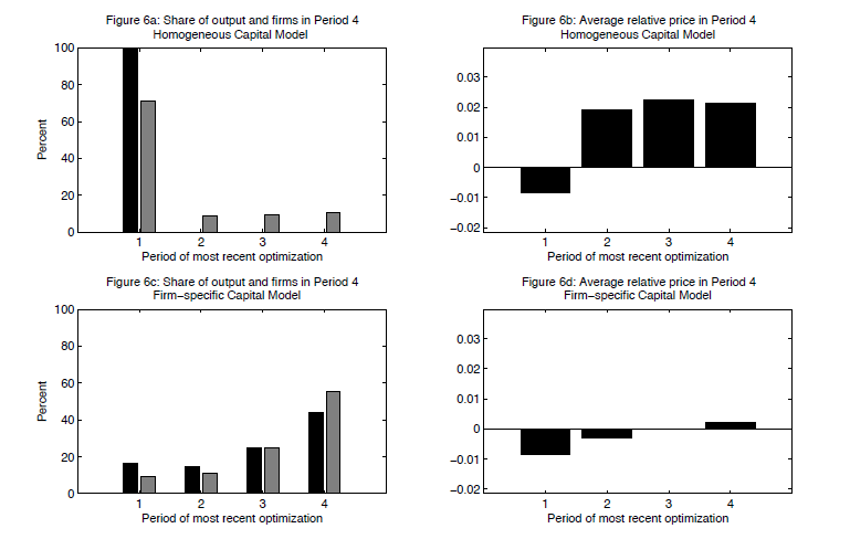
Data for Figure 6: Data Underlying Panel A
| a-axis | black bar | grey bar |
|---|---|---|
| 1.0000 | 131.7735 | 71.2646 |
| 2.0000 | -7.8267 | 8.5194 |
| 3.0000 | -11.9339 | 9.5379 |
| 4.0000 | -12.0130 | 10.6781 |
Data for Figure 6: Data Underlying Panel B
| a-axis | black bar |
|---|---|
| 1.0000 | -0.0085 |
| 2.0000 | 0.0192 |
| 3.0000 | 0.0225 |
| 4.0000 | 0.0213 |
Data for Figure 6: Data Underlying Panel C
| a-axis | black bar | grey bar |
|---|---|---|
| 1.0000 | 16.6260 | 8.9915 |
| 2.0000 | 14.5539 | 11.0789 |
| 3.0000 | 25.0009 | 24.7296 |
| 4.0000 | 43.8191 | 55.2000 |
Data for Figure 6: Data Underlying Panel D
| a-axis | black bar |
|---|---|
| 1.0000 | -0.0085 |
| 2.0000 | -0.0031 |
| 3.0000 | -0.0001 |
| 4.0000 | 0.0021 |
Figure 7: Features of the Distribution of Output and Prices Across Firms: Lower Demand Elasticity
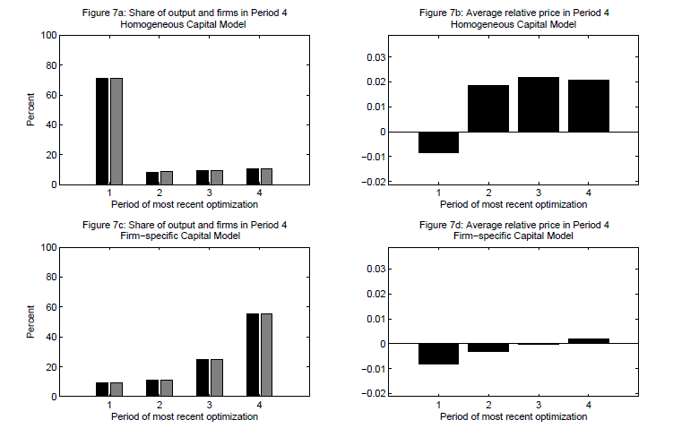
Data for Figure 7: Data Underlying Panel A
| a-axis | black bar | grey bar |
|---|---|---|
| 1.0000 | 131.7735 | 71.2646 |
| 2.0000 | -7.8267 | 8.5194 |
| 3.0000 | -11.9339 | 9.5379 |
| 4.0000 | -12.0130 | 10.6781 |
Data for Figure 7: Data Underlying Panel B
| a-axis | black bar |
|---|---|
| 1.0000 | -0.0085 |
| 2.0000 | 0.0192 |
| 3.0000 | 0.0225 |
| 4.0000 | 0.0213 |
Data for Figure 7: Data Underlying Panel C
| a-axis | black bar | grey bar |
|---|---|---|
| 1.0000 | 16.6260 | 8.9915 |
| 2.0000 | 14.5539 | 11.0789 |
| 3.0000 | 25.0009 | 24.7296 |
| 4.0000 | 43.8191 | 55.2000 |
Data for Figure 7: Data Underlying Panel D
| a-axis | black bar |
|---|---|
| 1.0000 | -0.0085 |
| 2.0000 | -0.0031 |
| 3.0000 | -0.0001 |
| 4.0000 | 0.0021 |
Bibliography
Altig, David, Lawrence J. Christiano, Martin Eichenbaum and Linde Jesper, 2004, Technical Appendix to 'Firm-Specific Capital, Nominal Rigidities and the Business Cycle'.
Altig, David, Lawrence J. Christiano, Martin Eichenbaum and Linde Jesper, 2005, 'Firm-Specific Capital, Nominal Rigidities and the Business Cycle', NBER Working Paper 11034.
Alves, Nuno, 2004, 'A Flexible View on Prices', Banco de Portugal Working Paper 2004-6.
Anderson, Gary S. and George Moore, 1985, 'A Linear Algebraic Procedure for Solving Linear Perfect Foresight Models,' Economic Letters 17, 247-52.
Ball, Laurence and David Romer, 1990, 'Real Rigidities and the Non-neultrality of Money,' Review of Economic Studies 57, 183-203.
Basu, Susanto, 1997, 'Intermediate Goods and Business Cycles: Implications for Productivity and Welfare', American Economic Review 85(3), 512-31.
Basu, Susanto, John Fernald and Matthew Shapiro, 2001, 'Productivity Growth in the 1990's: Technology, Utilization, or Adjustment?', Carnegie-Rochester Conference Series on Public Policy 55, 117-165.
Bierens, Herman J., 2004, Introduction to the Mathematical and Statistical Foundations of Econometrics, Cambridge University Press.
Bils, Mark and Pete Klenow, 2004, 'Some Evidence on the Importance of Sticky Prices,' Journal of Political Economy 112(5), 947 - 985.
Boldrin, Michele, Lawrence J. Christiano, and Jonas Fisher, 2001, 'Habit Persistence, Asset Returns and the Business Cycle,' American Economic Review 91(1), 149-166.
Bowman, David, 2003, 'Market Power and Inflation' Board of Governors of the Federal Reserve System, International Finance Discussion Papers number 783.
Calvo, Guillermo, 1983, 'Staggered Prices in a Utility-Maximizing Framework', Journal of Monetary Economics 12(3), 383-98.
Carvalho, Carlos, 2006, "Heterogeneity in Price Stickiness and the Real Effects of Monetary Shocks," Frontiers of Macroeconomics 2(1), Article 1.
Christiano, Lawrence J., 2002, 'Solving Dynamic Equilibrium Models by a Method of Undetermined Coefficients,' Computational Economics, October, 20 (1-2).
Christiano, Lawrence J., 2004, 'Firm-Specific Capital and Aggregate Inflation Dynamics in Woodford's Model,' manuscript, http://www.faculty.econ.northwestern.edu/faculty/christiano/research/firm specific/svensson.pdf.
Christiano, Lawrence J. and Martin Eichenbaum, 1992, 'Current Real-Business-Cycle Theories and Aggregate Labor-Market Fluctuations', American Economic Review 82 (3), 430-50.
Christiano, Lawrence J., Martin Eichenbaum, and Charles Evans, 1999, 'Monetary Policy Shocks: What Have We Learned and to What End?', Handbook of Macroeconomics, vol. 1A,eds., Michael Woodford and John Taylor, Amsterdam; New York and Oxford: Elsevier Science, North-Holland.
Christiano, Lawrence J., Martin Eichenbaum, and Charles. Evans, 2005, 'Nominal Rigidities and the Dynamic Effects of a Shock to Monetary Policy', Journal of Political Economy 113(1), 1-45.
Christiano, Lawrence J., and Terry Fitzgerald, 2003, 'The Band Pass Filter,' International Economic Review 44(2), 435-465.
Christiano, Lawrence J., Roberto Motto and Massimo Rostagno, 2004, 'The Great Depression and the Friedman-Schwartz Hypothesis,' Journal of Money, Credit and Banking 53(6), 1199-1204.
Christoffel, Kai, Gunter Coenen, and Andrew Levin, 2007, 'Identifying the Influences of Real and Nominal Rigidities in Aggregate Price-Setting Behavior,' Journal of Monetary Economics 54(8), 2439-2466.
de Walque, Gregory, Frank Smets and Raf Wouters, 2006, 'Firm-Specific Production Factors in a DSGE Model with Taylor Price Setting', International Journal of Central Banking 2(3), 107-154,.
DiCecio, Riccardo, 2009, 'Sticky Wages and Sectoral Labor Comovement,' Journal of Economic Dynamics and Control 33(3), 538-53.
Dotsey, Michael and Robert King, 2009, 'Pricing, Production and Persistence,' Journal of the European Economic Association 4(5), 893-928.
Edge, Rochelle M., Thomas Laubach and John C. Williams, 2003, 'The Responses of Wages and Prices to Technology Shocks,' Finance and Economics Discussion Series 2003-65. Washington: Board of Governors of the Federal Reserve System.
Eichenbaum, Martin and Jonas Fisher, 2007, 'Estimating the Frequency of Price Re-Optimization in Calvo-Style Models', Journal of Monetary Economics 54(7), 2032- 47.
Eichenbaum, Martin, Nir Jaimovich, and Sergio Rebelo, 2008, " Reference Prices and Nominal Rigidities," NBER Working paper 13829.
Erceg, Christopher J., Dale W. Henderson and Andrew T. Levin, 2000, 'Optimal Monetary Policy with Staggered Wage and Price Contracts,' Journal of Monetary Economics 46(2), 281-313..
Fisher, Jonas, 2006, 'The Dynamic Effects of Neutral and Investment-Specific Technology Shocks,' Journal of Political Economy 114 (3), 413-52.
Gali, Jordi, and Mark Gertler, 1999, 'Inflation dynamics: A structural econometric analysis,' Journal of Monetary Economics 44, 195-222.
Gali, Jordi, Mark Gertler, and J. David Lopez-Salido, 2001 "European Inflation Dynamics," European Economic Review 45 1237-70.
Gali, Jordi, J. David Lopez-Salido, and Javier Valles, 2002, 'Technology Shocks and Monetary Policy: Assessing the Fed's Performance', Journal of Monetary Economics 50(4), 723-43.
Gertler, Mark and John Leahy, 2008, "A Phillips Curve with an Ss Foundation," Journal of Political Economy 116 (June): 533-72.
Golosov, Michael., and Robert E. Lucas, 2007,: 'Menu Costs and Phillips Curves,' Journal of Political Economy,' 115, 171-199.
Huang, Kevin. X., 2006, "Specific Factors Meet Intermediate Inputs: Implications for the Persistence Problem," Review of Economic Dynamics 9, 483-507.
Justiniano, Alejandro and Giorgio Primiceri, 2008, 'The Time Varying Volatility of Macroeconomic Fluctuations,' American Economic Review 98(3), 604-41.
Kimball, Miles, 1995, 'The Quantitative Analytics of the Basic Neomonetarist Model,' Journal of Money, Credit and Banking 27 (4), part 2, 1241-77.
Klenow, Peter J. and Oleg Kryvtsov, 2008, 'State-Dependent or Time-Dependent Pricing: Does It Matter for Recent U.S. Inflation,' Quarterly Journal of Economics 123 (August), 863-904.
Klenow, Peter J. and Benjamin A. Malin, (2009), 'Microeconomic Evidence on Price Setting', manuscript, Stanford University.
Levin, Andrew T., J. David Lopez-Salido, Edward Nelson and Tak Yun, 2008, Macroeconometric Equivalence, Microeconomic Dissonance, and the Design of Monetary Policy, Federal Reserve Bank of St. Louis Working Paper number 2008-035.
Lindé, Jesper, 2005, 'Estimating New Keynesian Phillips Curves: A Full Information Maximum Likelihood Approach,' Journal of Monetary Economics 52(6), 1135-49.
Mackowiak, Bartosz and Frank Smets, 2008, 'On Implications of Micro Price Data for Macro Models', ECB Working Paper 960.
Mackowiak, Bartosz and Mirko Weiderholdt, 2009, 'Optimal Sticky Prices Under Rational Inattention', American Economic Review 99(3), 769-803.
Mankiw, N. Gregory, and Ricardo Reis, 2002, "Sticky Information versus Sticky Prices: A Proposal to Replace the New Keynesian Phillips Curve," Quarterly Journal of Economics 117 (November), 1295-1328.
Nakamura, Emi and Jon Steinsson, 2008, "Monetary Non-Neutrality in a Multi-Sector Menu Cost Model," NBER Working Paper 14001 (May).
Prescott, Edward, 1986, 'Theory Ahead of Business Cycle Measurement,' Federal Reserve Bank of Minneapolis Quarterly Review.
Rabanal, Pau and Juan F. Rubio-Ramírez, (2005), 'Comparing New Keynesian models of the Business Cycle: A Bayesian Approach', Journal of Monetary Economics 52, 1151-1166.
Reis, Ricardo, 2006, "Inattentive Producers," Review of Economic Studies 73, 793-821.
Rotemberg, Julio J. and Michael Woodford, 1997, 'An Optimization-Based Econometric Framework for the Evaluation of Monetary Policy,' National Bureau of Economic Research Macroeconomics Annual.
Sbordone, Argia M., 1998,"Prices and Unit Labor Costs: A New Test of Price Stickiness," IIES Seminar Paper no. 653, Stockholm University.
Sbordone, Argia, 2002, 'Prices and Unit Labor Costs: A New Test of Price Stickiness,' Journal of Monetary Economics 49 (2), pp. 265-292.
Shapiro, Matthew, and Mark Watson, 1988, 'Sources of Business Cycle Fluctuations,' NBER Macroeconomics Annual, 111-148.
Smets, Frank, and Raf Wouters, 2003, 'An Estimated Dynamic Stochastic General Equilibrium Model of the Euro Area,' Journal of the European Economic Association 1(5), 1123-1175.
Sims, Christopher A., 1994, 'A Simple Model for the Determination of the Price Level and the Interaction of Monetary and Fiscal Policy,' Journal of Economic Theory 4, 381-399.
Sims, Christopher A., 1998, "Stickiness," Carnegie-Rochester Conference Series on Public Policy, 49: 317-356.
Sims, Christopher A., 2003, "Implications of Rational Inattention," Journal of Monetary Economics 50: 665-690.
Schmitt-Grohe, Stefanie and Martin Uribe, 2004, 'Optimal fiscal and monetary policy under sticky prices,' Journal of Economic Theory 114, 198-230.
Sveen, Tommy, and Lutz Weinke, 2007a, 'Firm-Specific Capital, Nominal Rigidities, and the Taylor Principle,' Journal of Economic Theory 136(1), 729-37.
Sveen, Tommy, and Lutz Weinke, 2007b, 'Lumpy Investment, Sticky Prices and the Monetary Transmission Mechanism,' Journal of Monetary Economics 54(1), 23-36.
Woodford, Michael, 1996, 'Control of the Public Debt: A Requirement for Price Stability,' NBER Working Paper 5684.
Woodford, Michael, 2003, Interest and Prices: Foundations of a Theory of Monetary Policy, Princeton University Press.
Woodford, Michael, 2005, "Firm-Specific Capital and the New-Keynesian Phillips Curve,"International Journal of Central Banking 1(2): 1-46.
Woodford, Michael, 2008, "Information-Constrained State-Dependent Pricing," NBER Working paper 14620.
Yun, Tack, 1996, 'Nominal Price Rigidity, Money Supply Endogeneity, and Business Cycles,' Journal of Monetary Economics 37(2): 345 - 370.
Footnotes
1. We are grateful for the comments of David Andolfatto, Gadi Barlevy, Jesús Fernández-Villaverde, Andy Levin and Harald Uhlig. In addition we have benefitted from the reactions of the participants in the Third Banco de Portugal Conference in Monetary Economics, Lisbon, Portugal, June 10, 2004, the conference on Dynamic Models and Monetary Policymaking, September 22-24, 2004, held at the Federal Reserve Bank of Cleveland, and the conference "SDGE Models and the Financial Sector" organized by Deutsche Bundesbank in Eltville, November 26-27, 2004. We are also grateful for the comments of the participants in the 'Impulses and Propagations' workshop of the NBER Summer Institute in the week of July 19, 2004 and the conference "Macroeconomics and Reality, 25 Years Later" held in Barcelona, April 1-2, 2005. Finally, we are particularly grateful for the insights and for the research assistance of Riccardo Dicecio. The views expressed in this paper are solely the responsibility of the authors and should not be interpreted as reflecting the views of the Board of Governors of the Federal Reserve System, Federal Reserve Bank of Atlanta, or of any other person associated with the Federal Reserve System. Return to text
2. Federal Reserve Bank of Atlanta. Return to text
3. Northwestern University, National Bureau of Economic Research, and Federal Reserve Banks of Chicago, Atlanta and Minneapolis. Return to text
4. Northwestern University, National Bureau of Economic Research, and Federal Reserve Banks of Chicago and Atlanta. Return to text
5. Board of Governors of the Federal Reserve System and CEPR. Return to text
6. For example, Eichenbaum and Fisher (2007) find that estimated versions of Calvo pricing models with indexing to lagged inflation imply that firms reoptimize prices roughly once every six quarters. Smets and Wouters' (2003) estimated model implies that firms reoptimize prices on average once every nine quarters. Return to text
7. See for example the estimates in Rabanal and Ramírez (2005) for the post 1982 era or the NBER working paper 10617 version of Eichenbaum and Fisher (2007). Return to text
8. For example in calibrating their model to the micro data, Golosov and Lucas (2007) select parameters to ensure that firms change prices on average once every 1.5 quarters. Return to text
9. To maintain contact with the bulk of estimated new Keynesian models we assume that firms index prices to lagged inflation. The NBER working paper 10617 version of Eichenbaum and Fisher (2007) establishes that the introduction of firm specific capital has similar effects in models with and without indexation to lagged prices Return to text
10. See also Dicecio (2009) for a multi-sectoral general equilibrium model which allows for the same shocks that we consider. Also Edge, Laubach and Williams (2003) consider a general equilibrium model with two types of technology shocks. Galí, López-Salido and Vallés (2003) consider neutral technology shocks only. Return to text
11. For early discussions of this idea, see Ball and Romer (1990) and Kimball (1995). Return to text
12. A closely related assumption that generates an upward sloping marginal cost curve is that there are internal costs of adjusting capital. Return to text
13. See Levin, Lopez-Salido, Nelson and Yun (2008) who emphasize this point and analyze the nature of optimal policy in the non-linear versions of the two models. Return to text
14. See Ball and Romer (1990) and Kimball (1995) for an early discussion of this point. Return to text
15. The quality of our estimation strategy depends on the ability of identified VARs to generate reliable estimates of the dynamic response of economic variables to shocks. In an appendix, available upon request, we evaluate the reliability of VAR methods in our application by means of Monte Carlo simulation methods. We find that the Monte Carlo performance of our VAR based estimates of impulse response functions is very good. Return to text
16. Our strategy for identifying technology shocks follows Fisher (2006). Return to text
17. Since our paper was written, an interesting literature has arisen incorporating firm-specific capital into analyzes of price setting. See for example Christoffel, Coenen, and Levin (2007), de Walque, Smets and Wouters (2006) Eichenbaum and Fisher (2007), and Sveen and Weinke (2007a, 2007b).
18. The constant of proportionality is the probability of the relevant state of the world. Return to text
19. See Christiano (2004) for a discussion of the solution to firm-specific capital models in simpler settings. Return to text
20. Justiniano and Primiceri (2008) argue that conditional heteroscedasticity in fundamental shocks is important for explaining the 'Great Moderation'. Similar arguments have been made by CEE (1999) and Smets and Wouters (2007). Return to text
21. Nominal gross output is measured by GDP, real gross output is measured by GDPC96 (real, chain-weighted GDP). Nominal investment is PCDG (household consumption of durables) plus GPDI (gross private domestic investment). Nominal consumption is measured by PCND (nondurables) plus PCESV (services) plus GCE (government expenditures). Real private domestic investment is given by GPDIC96. Real private consumption expendutures are given by PCEC96. Our MZM measure of money is MZMSL. Variables were converted into per capita terms by CNP16OV, a measure of the US civilian non-institutional population over age 16. A measure of the aggregate price index was obtained from the ratio of nominal to real output, GDP/GDPC96. Capacity utilization is measured by CUMFN, the manufacturing industry's capacity index. The interest rate is measured by the federal funds rate, FEDFUNDS. Hours worked is measured by HOANBS (Non-farm business hours). Hours were converted to per capita terms using our population measure. Nominal wages are measured by COMPNFB, (nominal hourly non-farm business compensation). This was converted to real terms by dividing by the aggregate price index. Return to text
22. We also re-estimated the VAR and the structural model using as our measures of hours and productivity, private business hours and business sector productivity, respectively. In these estimation runs, we measure consumption and output as private sector consumption and private sector output, respectively. Taking sampling uncertainty, we find that our results are robust to these alternatives data measures. Return to text
23. The estimation period for the vector
autoregression drops the first ![]() quarters, to
accommodate the
quarters, to
accommodate the ![]() lags. Return to text
lags. Return to text
24. See Bierens (2004) for the formulas used and for a discussion of the asymptotic properties of the lag length selection criteria. Return to text
25. The confidence intervals are symmetric about our point estimates. They are obtained by adding and subtracting 1.96 times our estimate of the standard errors of the coefficients in the impulse response functions. These standard errors were computed by bootstrap simulation of the estimated model. Return to text
26. Alves (2004) also finds that inflation drops after a positive neutral technology shocks using data for non-U.S. G7 countries Return to text
27. We found that the analog statistics computed using the Hodrick-Prescott filter yielded essentially the same results. We computed this as follows:
where
28. In our model, the steady state share
of labor income in total output is ![]() This
result reflects our assumption that profits are zero in steady
state. Return to text
This
result reflects our assumption that profits are zero in steady
state. Return to text
29. Adding the years 2002 - 2008 makes
little difference to our estimate of
![]() and
and ![]() Return to text
Return to text
30. For the 1982-2008 period, the
investment deflator drops on average by -2.3 percent.
Over the same sample period GDP per capita growth was 1.75 percent at an annualized rate, implying that ![]() is less than one. Return
to text
is less than one. Return
to text
31. The average annual growth rate of MZM over the sample period 1982-2008 and 1959-2008 is 2 and 1.7 percent, respectively. Return to text
32. This number was obtained using the algorithm discussed in ACEL (2004). Return to text
33. Prescott (1986) actually reports a
standard deviation of 0.763 percent. However, he
adopts a different normalization for the technology shock than we
do, by placing it in front of the production function. By
assumption, the technology shock multiplies labor directly in the
production and is taken to a power of labor's share. The value of
labor's share that Prescott uses is 0.70. When we
translate Prescott's estimate into the one relevant for our
normalization, we obtain
![]() . Return to text
. Return to text
34. This estimate is consistent with results in the literature. See Eichenbaum and Fisher (2007) and the references therein. Return to text
35. We set
![]() Also, we measure marginal
productivity by labor's share in GDP. In our model this is the
correct measure if fixed costs are zero. This measure is
approximately correct here, since our estimate of
Also, we measure marginal
productivity by labor's share in GDP. In our model this is the
correct measure if fixed costs are zero. This measure is
approximately correct here, since our estimate of ![]() is close to zero. Return to
text
is close to zero. Return to
text
36. Eichenbaum and Fisher (2007) argue
that their estimates of ![]() are robust to
alternative measures of marginal cost. Return to text
are robust to
alternative measures of marginal cost. Return to text
37. We obtain the same results whether we
work with
![]() or with
or with
![]() Return to text
Return to text
38. See, for example, Ball and Romer (1990), CEE (2005), Dotsey and King (2009), Galí and Gertler (1999), Lindé (2005) and Smets and Wouters (2003). Return to text
39. This is a straightforward implication
of the homogeneous capital model discussed above, according to
which
![]() Return to text
Return to text
40. Marginal costs could be increasing because of firm-specificity of other factors of production or costs of adjusting production inputs. Return to text
41. One measure of the degree of inequality in production is provided by the Gini coefficient. In periods 4, 8 and 16, these are 0.12, 0.15 and 0.26 for the firm-specific capital version of the model.
42. The behavior of firms when capital is
firm specific is not substantially affected by the higher value of
![]() Return to text
Return to text
This version is optimized for use by screen readers. Descriptions for all mathematical expressions are provided in LaTex format. A printable pdf version is available. Return to text