
Board of Governors of the Federal Reserve System
International Finance Discussion Papers
Number 1040r, June 2012 --- Screen Reader
Version*
Missing Import Price Changes and Low Exchange Rate Pass-Through
NOTE: International Finance Discussion Papers are preliminary materials circulated to stimulate discussion and critical comment. References in publications to International Finance Discussion Papers (other than an acknowledgment that the writer has had access to unpublished material) should be cleared with the author or authors. Recent IFDPs are available on the Web at http://www.federalreserve.gov/pubs/ifdp/. This paper can be downloaded without charge from the Social Science Research Network electronic library at http://www.ssrn.com/.
Abstract:
A large body of empirical work has found that exchange rate movements have only modest effects on inflation. However, the response of an import price index to exchange rate movements may be underestimated because some import price changes are missed when constructing the index. We investigate downward biases that arise when items experiencing a price change are especially likely to exit or to enter the index. We show that, in theoretical pricing models, entry and exit have different implications for the timing and size of these biases. Using Bureau of Labor Statistics (BLS) microdata, we derive empirical bounds on the magnitude of these biases and construct alternative price indexes that are less subject to selection effects. Our analysis suggests that the biases induced by selective exits and entries are modest over typical forecast horizons. As such, the empirical evidence continues to support the conclusion that exchange rate pass-through to U.S. import prices is low.
Keywords: Exchange rate pass-through, import prices, item replacement
JEL classification: F31, F41, E30, E01, C81
In conducting monetary policy, central bankers are interested in how much exchange rate movements affect the prices of imported goods ("exchange rate pass-through") as fluctuations in these prices can, in turn, affect domestic prices and output. Commonly, exchange rate pass-through is measured by regressing changes in published import price indexes on changes in trade-weighted exchange rate indexes along with other explanatory variables. Using these regressions, researchers have estimated low rates of exchange rate pass-through for the United States. Recent estimates (for example, Campa and Goldberg [2005], and Marazzi and Sheets [2007]) suggest that, following a 10 percent depreciation of the dollar, U.S. import prices increase about 1 percentage point in the contemporaneous quarter and an additional 2 percentage points over the next year, with little if any subsequent increases. These low estimates have led several authors to formulate theories which generate incomplete pass-through.1
In a recent paper, Nakamura and Steinsson (2011) argue that actual long-run pass-through is substantially higher than these standard estimates because published price indexes are missing price changes associated with item replacement. In their words, "[if] the prices of new products entering the index have already adjusted to exchange rate movements ... [then] the response of these prices to movements in exchange rates ... will be `lost in transit' (i.e., neither picked up by an observed price change of the exiting nor entering product)." They derive an adjustment factor for standard long-run pass-through estimates under specific assumptions regarding the nature of item substitutions and the way firms set prices. They find that measured pass-through is underestimated by a factor of almost two, implying that exchange rate pass-through to U.S. import prices is much more complete in the long run than was previously thought.
Our paper reassesses this conclusion by developing a general framework for understanding how sample exits and sample entries--in conjunction with pricing assumptions--impact measured pass-through, and by proposing and implementing new ways of gauging the biases in standard estimates. Throughout our discussion, we emphasize the implications of item substitutions over the first couple years following an exchange rate shock, as such a short-term horizon is most commonly employed by forecasters and is especially useful for discriminating among theoretical models.2 Our conceptual framework captures the possibility that an item whose price is about to change is more likely than others to leave the index (resulting in a "selective exit") and that an item whose price recently changed is more likely than others to join the sample (resulting in a "selective entry"). We demonstrate that the effects of item replacement on measured pass-through crucially depend on the nature of both exits and entries of items. In turn, the magnitude of these effects can be sensitive to pricing assumptions and the time horizon of interest. By contrast, the presence of real rigidities is typically of limited consequences. In presenting these findings, we substantially expand the analysis of Nakamura and Steinsson, who are primarily concerned with the long-run effects of item substitutions and do not explicitly model sample exits.
Our theoretical work explores the implications of selective exits and selective entries under two popular price-setting mechanisms, Calvo and menu-cost, which together span a wide range of pricing behavior relevant for understanding pass-through dynamics. The most consequential situation is when price changes are missed both when items exit the sample and when they enter it. In such a case of selective exits and selective entries, standard pass-through estimates omit a roughly constant fraction of the actual exchange response, a finding that applies to all time horizons and both pricing models. When only exits are subject to a selection bias, the estimation bias as a share of the cumulative response is largest initially, but then falls over time as items that have yet to respond to the exchange rate are brought into the sample. This offsetting effects is largest in the Calvo model due to its relatively slow transmission of shocks. When only entries are subject to a selection bias, measured pass-through is initially unbiased, but a bias then gradually appears as entering items prove insensitive to past exchange rate movements. The bias grows largest in the Calvo model because of its relatively slow pass-through of shocks, which means that item substitutions are likely to take place before pass-through is complete.
In the U.S. import price index, there is about one item replacement for every 5 price changes and as reported by Nakamura and Steinsson (2011) 40 percent of items leave the sample without ever experiencing a price change. The potential for economically important biases in standard pass-through regressions is thus material, provided that many item exits and entries are subject to a selection effect. However, based on a range of empirical exercises, we conclude that the biases induced by selective exits and entries, although a concern and worthy of continued research, do not materially alter the literature's view that pass-through to U.S. import prices is low over typical forecast horizons. To inform our judgement, we first use BLS microdata to derive empirical bounds on the price level response to an exchange rate shock. To do so, we calibrate our Calvo and menu-cost models to match key features of exchange rate movements, item substitutions, and individual price adjustments, then we recover the model-implied correction factors. Our baseline empirical estimate of pass-through to imported finished goods prices after two years is 0.24. After correcting for the most severe case of selective exit and selective entry consistent with the data, our pass-through estimate rises only to 0.28.
We next use BLS microdata to construct alternative price indexes in which the inclusion of newly sampled items in the index is delayed. We formally prove that this delaying procedure can substantially mitigate the selective entry bias over typical forecast horizons in a Calvo model. The intuition is that when entries are selective, added items are too insensitive to past exchange rate movements; simply delaying their entry in the index reduces this selection effect by allowing the distribution of added items to mix. As such, theory predicts that if selective entries were frequent, then these alternative prices should imply higher pass-through rates. However, when we estimate pass-through rates using these alternative price indexes, we do not find any evidence of bias reduction. This result casts further doubt on the empirical relevance of selective entries.
The remainder of the paper is structured as follows. Section 1 describes the sample of items used by the BLS to compute import price inflation and provides an overview of item exits and entries. Section 2 introduces the baseline Calvo and menu-cost models that we use to illustrate the nature of the various biases and to gauge their quantitative importance. Section 3 presents the possible biases associated with selection effects in sample exit and entry. Section 4 explores the empirical relevance of these biases by computing bounds on standard pass-through estimates and by constructing an alternative price index that mitigates these biases. Section 5 concludes.
1 Nature and Occurrence of Item Exits and Entries
Our study focuses on changes to the BLS import price sample, not on changes to the population (universe) of imported items.3 For clarity, we reserve the terms "exit" and "entry" for changes in the composition of the sample. Throughout the presentation of the data and subsequent model-based analysis, we are concerned with the possibility that micro price changes tend to take place just after items exit the sample or shortly before items enter the sample, so that part of the price response to shocks is censored. We define a "selective exit" as the subtraction of an item from the sample that is triggered by its price being about to change, and a "selective entry" as a systematic addition to the sample of an item that recently experienced a price change. By contrast, a "random exit" and a "random entry" are, respectively, the subtraction from and the addition to the sample of an item without regards to its pricing characteristics.
With the above terminology in mind, the remainder of this section provides background information about the construction of the import price indexes used in standard pass-through regressions, emphasizing the nature and occurrence of sample exits and entries, their treatment by the BLS, the potential for selection biases, and their relationship to micro price adjustments.
1.1 The International Price Program
Given identical data to Gopinath and Rigobon (2008) and Nakamura and Steinsson (2011), we rely on their work to convey the details of the BLS' International Price Program (IPP) protocol and sample, as well as on the BLS Handbook of Methods. In brief, import prices are collected through a monthly survey of U.S. establishments. The sample consists of rolling groups of items, each item having a sampling duration of about three years, on average.4 The IPP chooses its firms and items based on a proportional-to-size sampling frame with some degree of oversampling of smaller firms and items.5 Respondents must provide prices for actual transactions taking place as closely as possible to the first day of the month. In total, we observe the price of approximately 13,000 imported items per month from September 1993 to July 2007. For the purpose of computing our sample statistics, and consistent with previous studies, we carry forward the last reported price to fill in missing values, effectively overwriting IPP price imputations and firm estimates of prices in non-traded periods. We also restrict our sample to U.S. dollar transactions, which account for about 90 percent of all observations.
1.2 Nature of Exits and Entries
BLS price collectors take note when an item exits the sample and assign the retiring item one of the following codes: (1) regular phaseout, (2) accelerated phaseout, (3) sample dropped, (4) refusal, (5) firm out of business, (6) out of scope, not replaced, and (6) out of scope, replaced. Codes (1) through (3) indicate that item exit is driven primarily by the phaseout schedule of the IPP sampling protocol. Codes (4) and (5) describe situations in which price collection is impossible because the survey respondent refuses to respond or ceases to operate, even though the exiting items may continue to be traded in the universe. Codes (6) and (7) are those instances in which price quotes are unavailable because the item ceases to be traded by importers.6
The purpose of item phaseouts is to keep the sample representative of the universe of items; the BLS resamples approximately half of its disaggregated product categories every two years and typically plans to retire items five years after their entry. An item may retire early if it is insufficiently traded. We see such exists, given their planned nature, as unlikely to be selective. Contrary to phaseouts, refusals and importers going out of business are not foreseen events. Nevertheless, we view the risk that such exits systematically mask individual price adjustments as relatively modest, as there are several factors unrelated to micro price adjustments that could trigger them. Exits associated with items becoming out of scope likely present the greatest risk of masking price adjustments. For example, an importer could cease to order an item when faced with a price increase eating away its profit margins. The item could also exit because the foreign producer is adjusting the item's effective price through a change in its characteristics. Other situations leading to out-of-scope items may be unrelated to micro price adjustments. For example, the importer may be curtailing the range of varieties it has on offer in order to streamline inventory management.
It is worthwhile to note that exits are not generally accompanied by the simultaneous entry of a newly sampled item. When an item suddenly becomes out of scope, BLS price analysts ask the reporting firm whether it can provide another item that meets the sampling criteria of the exiting item. When it is possible, the BLS may link the price of the entering and exiting items through a one-time quality adjustment, in which case the change in the effective price is properly recorded. However, that is a relatively infrequent practice. In other instances, the firm may provide an alternative item meeting the BLS sampling needs, though that item is recorded as a separate entry. More often, when no item with similar characteristics is available in the same establishment, or when the planned phaseout date is within the next 18 months, the BLS simply waits until the next biennial sample redrawing. The lag between an unplanned exit and the subsequent item entry can thus be fairly long. Even in the case of planned phaseouts, BLS protocol does not necessitate synchronizing exit and entry.7
Notwithstanding the fact that exits and entries are staggered, the size of the IPP sample has been roughly constant since 1993 as the gross number of exits has typically been matched by a corresponding number of entries. The BLS uses probability sampling techniques to select establishments within broad strata of items, and then to select product categories within each stratum-establishment combination. A BLS field agent next conducts an interview with the establishment to select specific items. Probability sampling may be used at that stage. In general, special efforts are made to ensure that selected items are traded regularly, which implies that higher-volume items with established price histories are more likely to be selected.
In principle, the BLS's decision to sample a given item from within the universe should be unrelated to the timing of that item's price changes. Indeed, our reading of the BLS methodology is that the risk of selective entries is somewhat low, especially for those items entering the sample through planned sample redrawing. The risk of selective entries is arguably larger for items entering the sample concurrently with or immediately after an unplanned exit when no quality adjustment is made. Our assessment that the risk of selective entries is relatively low stands in contrast with the working assumption in Nakamura and Steinsson (2011) that all entries are selective. For this reason, we will illustrate the magnitude of the bias in our quantitative analysis below under the full range - 0 to 100 percent - of possible selection effects.
1.3 Accounting for Exit and Entry
For a given month ![]() , let
, let ![]() and
and
![]() be the number of price items exiting
and entering the sample, respectively. These items cannot beused in
the computation of inflation at month
be the number of price items exiting
and entering the sample, respectively. These items cannot beused in
the computation of inflation at month ![]() because their
price in either month
because their
price in either month ![]() or
or ![]() is
missing. For items whose price is available in both month
is
missing. For items whose price is available in both month
![]() and
and ![]() , let
, let
![]() and
and
![]() be the number of observations
with a price change and no price change, respectively. We define
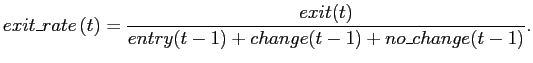
the exit rate as
be the number of observations
with a price change and no price change, respectively. We define
the exit rate as
The denominator in the above expression is the number of items
whose price was collected in month ![]() . The exit
rate thus measures the fraction of items present in the sample at
the end of month
. The exit
rate thus measures the fraction of items present in the sample at
the end of month ![]() that leaves in the next month.
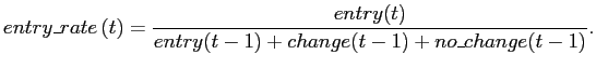
Analogously, the entry rate is measured as
that leaves in the next month.
Analogously, the entry rate is measured as
The fourth through seventh columns of table 1 show summary statistics about exits and entries over the period October 1995 to April 2005 for finished goods categories.8 For industry groupings, we use the Bureau of Economic Analysis 3-digit Enduse classification to bring descriptions of the microdata closer to the groups of goods commonly used in aggregate pass-through regressions (for instance, Bergin and Feenstra (2009) and Marazzi, et al. (2005)). In aggregating up from unique items in a given month to industry-level statistics, we weight each measure by its importance to overall U.S. import purchases.9 We aggregate the measures defined above in two stages: first, by computing unweighted statistics for each Enduse category in each month. Then, we aggregate across categories and time periods using the 2006 import sales value of each Enduse category.10
The rates of item exits and entries are both approximately 3 percent, indicating that the average size of the IPP sample remained about the same over the course of the sample. However, the steadiness of the overall sample size hides a degree of heterogeneity in exit and entry rates at the Enduse product level. For instance, computers and semiconductors (Enduse 213) had an entry rate of 5.0 percent, nearly twice that of agricultural machinery and equipment (Enduse 212). Certain categories (like computers) expanded over the course of the sample as evidenced by higher entry rates relative to exit rates. Differences in net entries likely reflect the changing trade intensity of certain categories over the course of the sample. Exiting items coded as out of scope, which we see as presenting the highest risk of selective exits, accounted for half (1.5 percentage points) of the total exit rate. Enduse categories with a relatively high share of out-of-scope exits include computers and semiconductors, home entertainment equipment, as well as trucks and buses.
By definition, a selective exit entails a price change concurrent with an item leaving the sample. This pattern suggests that the rate of selective exit should vary over time along with macroeconomic variables triggering price adjustments. Evidence of this phenomenon in scanner data is provided by Broda and Weinstein (2010) in their analysis of barcode creation and destruction over the business cycle. To see if exits of imported goods similarly respond to the exchange rate, the top panel of figure 1 presents the time series of the exit rate restricted to out-of-scope items along with an index of the broad nominal dollar.11 This measure is very close to the "endogenous exit" measure reported in Berger et al. (2009), with the minor difference that we also exclude exits resulting from aggregate refusals and out-of-business. The series is flat at about 1 percent throughout most of the early periods with a transient peak at the beginning of 2000. Then, the out-of-scope rate rises by about 50 basis points in 2003 through 2005. These three prominent features of the time series (i.e., flatness or slight decline early, peak in 2000, and uptick in 2003-5) correspond inversely to the pattern of the broad nominal dollar index, shown in black. The intuition for this relationship is straightforward: as the dollar depreciates, the profitability and viability of a higher proportion of imported items is adversely affected, leading firms to pull the items before the end of their scheduled sample life. We view this evidence as suggestive that exits may, in fact, occur in tandem with price changes.
The occurrence of exits related to factors other than items falling out of scope, which we see as presenting a relatively low risk of selection bias, varies far less systematically with the exchange rate. Rather, the random exit series exhibits the fairly normal pattern of peaks every two years (i.e., the end of 1996, 1998, 2000, 2002, and 2004), which is in line with the biennial shuffling of IPP items. For the most part, the overall entry rate shows a similar pattern with peaks in the middle of the year in 1997, 1999, and so on. Of note, similarly to the out-of-scope exit rate, the rate of overall entry also ticks up towards the end of the sample.
We also note that the timing of the changes in out-of-scope exit rates and, to a lesser extent, in entry rates, does not seem to account for the decline in measured exchange rate pass-through documented in the literature, which has roughly halved since the 1980's. The decrease in pass-through took place primarily in the 1990's, preceding the upticks in exit rates by quite a few years.
1.4 Micro Price Adjustments
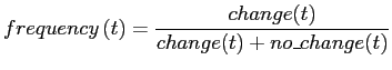
As will be made clear in the next section, the quantitative implication of selective exits and selective entries can be sensitive to the nature of the price-setting frictions giving rise to infrequent and lumpy nominal price adjustments. It will be convenient for our discussion to define the observed frequency of individual price changes as
 .
.The overall weighted incidence of price changes for finished goods is estimated to be 6.2 percent. The analogous statistic for the entire IPP import sample (i.e., additionally including industrial supplies, foods, feeds and beverages) is 15.3 percent.12 These levels are consistent with the weighted average of 14.1 percent in Nakamura and Steinsson (2011) and the median of 15 percent in Gopinath and Rigobon (2008). The average absolute (nonzero) price change is 6.7 percent for finished goods and 8.0 percent overall, in line with the mean overall estimate of 8.2 percent in Gopinath and Rigobon (2008). Here, again, there is significant dispersion across categories with items belonging to computers and peripherals (Enduse 213) having an average price change of 9.6 percent, compared to 2.0 percent for passenger cars (Enduse 300).
1.5 Other Data Considerations
We conclude the data description by mentioning two additional elements important for the interpretation of the results. First, in any given month, prices are missing for about 40 percent of items in the sample, which could reflect the absence of a transaction or simply reporting issues. Second, nearly half of all observations in the BLS sample refer to items that are traded between affiliates or entities of the same company. Although the BLS prefers that these intra-company transfer prices be market-based or market-influenced, some have expressed concern over whether these prices play the same allocative role as market transactions. Excluding intra-company transfer prices from the sample has a negligible impact on our analysis because intra-firm and market transactions have roughly similar entry rates, exit rates, and frequency of price changes. See Neiman (2010) and Gopinath and Rigobon (2008) for a comparison of intra-firm and market transactions.
2 Pass-Through and Micro Price Adjustments: A Baseline Case
This section introduces the baseline Calvo and menu-cost models that we will use to illustrate the nature of the various selection biases and how they interact with the frequency of prices changes. As we will show, judgement on the quantitative importance of the biases is sensitive to the price-setting mechanism one sees as best representing the data-generating process. Although the Calvo and menu-cost models are only two of the many price-setting mechanisms proposed in the literature, they illustrate the point that the severity of the biases often relates to the frequency of price changes and, more generally, to the speed at which exchange rate movements are passed-through to import prices.
2.1 Economic Environment
We consider the following data-generating process for the change
in the price (in logs) of an imported item ![]() at
period
at
period ![]() ,
,
![\begin{displaymath} \Delta p_{it}=\left \{ \begin{array}[c]{cc} 0 & \text{if }\mathcal{I}_{it}^{f}=0\ u_{it}+\beta \Delta x_{t}+\varepsilon_{it} & \text{if }\mathcal{I}_{it}^{f}=1 \end{array}\right. . \end{displaymath}](img18.gif)
Given the opportunity (or decision) to change its price, a firm
sets
![]() equal to the sum of (a) the
amount of price pressure inherited from previous periods,
equal to the sum of (a) the
amount of price pressure inherited from previous periods,
![]() , (b) the change in the exchange rate,
, (b) the change in the exchange rate,
![]() , and (c) the contribution of a
(mean-zero) idiosyncratic factor,
, and (c) the contribution of a
(mean-zero) idiosyncratic factor,
![]() . The occurrence of a price
change is marked by the indicator variable
. The occurrence of a price
change is marked by the indicator variable
![]() . The price deviation
carried to the beginning of the next period is given by
. The price deviation
carried to the beginning of the next period is given by
![\begin{displaymath} u_{it+1}=\left \{ \begin{array}[c]{cc} u_{it}+\beta \Delta x_{t}+\varepsilon_{it} & \text{if }\mathcal{I}_{it}^{f}=0\ 0 & \text{if }\mathcal{I}_{it}^{f}=1 \end{array}\right. . \end{displaymath}](img24.gif)
If the firm does not change its price, then the aggregate and
idiosyncratic shocks occurring in period ![]() are
simply added to the amount of price pressure that had already
cumulated. If the firm adjusts its price, then the price is set to
the optimum and no price pressure is carried into the next
period.13 The set up so far is quite general
and not specific to import prices. One could, for example,
interpret
are
simply added to the amount of price pressure that had already
cumulated. If the firm adjusts its price, then the price is set to
the optimum and no price pressure is carried into the next
period.13 The set up so far is quite general
and not specific to import prices. One could, for example,
interpret
![]() as the contribution of aggregate
shocks, such as wage inflation, to a firm's reset price. In what
follows, we will simply assume that
as the contribution of aggregate
shocks, such as wage inflation, to a firm's reset price. In what
follows, we will simply assume that
![]() can be represented by an
can be represented by an
![]() process,
process,
with Gaussian innovations, ![]() .
.
We are ultimately interested in the impact of exchange rate movements on import prices in general. To this end, we define aggregate price inflation as the average change in item prices,
Suppose that the econometrician estimates a linear model containing
![]() lags of the aggregate variable,
lags of the aggregate variable,
|
(1) |
where ![]() is an error term. In what follows, we
explore how various assumptions about the timing of nominal
adjustments impact the estimated regression coefficients.
is an error term. In what follows, we
explore how various assumptions about the timing of nominal
adjustments impact the estimated regression coefficients.
2.1.1 Calvo Model
In the Calvo model, the decision to change the price is
exogenous to the firm. The indicator variable
![]() is a random variable
taking the value
is a random variable
taking the value ![]() with constant probability
with constant probability
![]() , and 0 with probability
, and 0 with probability ![]() . This assumption has strong implications for the dynamic
responses of import prices to exchange rate movements. It is
convenient to consider the case in which innovations to the
exchange rate,
. This assumption has strong implications for the dynamic
responses of import prices to exchange rate movements. It is
convenient to consider the case in which innovations to the
exchange rate,
![]() , are uncorrelated over time
(
, are uncorrelated over time
(![]() ), as it allows us to derive analytical
expressions for the regression coefficients.
), as it allows us to derive analytical
expressions for the regression coefficients.
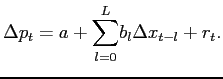
As appendix A shows (in a more general environment), the (plim) linear estimate ofis
| (2) |
Intuitively, for a movement in the exchange rate ![]() periods earlier to impact an item's price today, the firm must be
given the opportunity to adjust its price today (probability
periods earlier to impact an item's price today, the firm must be
given the opportunity to adjust its price today (probability
![]() ) and no price change must have occurred in
each of the previous
) and no price change must have occurred in
each of the previous ![]() periods (probability
periods (probability
![]() in each period). Otherwise, the current
price would already reflect
in each period). Otherwise, the current
price would already reflect
![]() . The Calvo model provides a
textbook example of a geometric lag model in which the coefficient
on the explanatory variable decays exponentially with the number of
lags. Summing up the (plim) coefficients in the regression, we get
. The Calvo model provides a
textbook example of a geometric lag model in which the coefficient
on the explanatory variable decays exponentially with the number of
lags. Summing up the (plim) coefficients in the regression, we get
which converges to ![]() as
as
![]() . Thus, although the
effects of an exchange rate shock never are passed-through fully to
import prices, we can nevertheless approximate
. Thus, although the
effects of an exchange rate shock never are passed-through fully to
import prices, we can nevertheless approximate ![]() (the "long-run" pass-through) as the sum of the
regression coefficients with an arbitrary degree of precision.
(the "long-run" pass-through) as the sum of the
regression coefficients with an arbitrary degree of precision.
2.1.2 Menu-Cost Model
In the menu-cost model, the decision t![]() o change the price is the
result of a cost-benefit analysis performed by the firm. As shown
by Sheshinski and Weiss (1977), it is optimal for the firm to keep
its price unchanged if the deviation from the reset price,
,
falls within a certain range. One can show that, to a first-order
approximation, this range of inaction is symmetric around the price
that sets the price pressure to zero (see Gopinath and Itskhoki,
2010, for a formal derivation). We thus approximate the decision to
change the price as
o change the price is the
result of a cost-benefit analysis performed by the firm. As shown
by Sheshinski and Weiss (1977), it is optimal for the firm to keep
its price unchanged if the deviation from the reset price,
,
falls within a certain range. One can show that, to a first-order
approximation, this range of inaction is symmetric around the price
that sets the price pressure to zero (see Gopinath and Itskhoki,
2010, for a formal derivation). We thus approximate the decision to
change the price as
![\begin{displaymath} \mathcal{I}_{it}^{f}=\left \{ \begin{array}[c]{cc} 0 & \text{if }\left \vert u_{it}+\beta \Delta x_{t}+\varepsilon_{it}\right \vert \leq K\ 1 & \text{if }\left \vert u_{it}+\beta \Delta x_{t}+\varepsilon_{it}\right \vert >K \end{array}\right. . \end{displaymath}](img53.gif)
Unfortunately, analytical results are challenging to derive for
the menu-cost model unless one is willing to make stringent
assumptions (see Danziger (1999) and Gertler and Leahy (2008) for
examples). However, the assumptions required for tractability seem
less suitable here. Therefore, we will proceed by simulations to
illustrate our main points. Note that the decision to change the
price now depends on the value of ![]() : The
larger the pass-through coefficient for a given
: The
larger the pass-through coefficient for a given ![]() ,
the more a shock to the exchange rate is likely to trigger a price
adjustment. More generally, the more shocks are large and
persistent (and thus associated with relatively large benefit of
adjusting the price), the more likely is a firm to change the price
immediately. The estimated coefficients in equation 1 are thus
sensitive to the particular realization of the shocks in the
menu-cost model.
,
the more a shock to the exchange rate is likely to trigger a price
adjustment. More generally, the more shocks are large and
persistent (and thus associated with relatively large benefit of
adjusting the price), the more likely is a firm to change the price
immediately. The estimated coefficients in equation 1 are thus
sensitive to the particular realization of the shocks in the
menu-cost model.
2.2 Calibration of the Models
We first set the mean, standard deviation, and autoregressive
coefficient of exchange rate innovations to match the corresponding
moment of the broad dollar index computed by the Federal Reserve
from January 1995 to March 2010. The standard deviation of monthly
(end-of-period) exchange rate movements was 1.5 percent over that period, with no apparent drift. Exchange rate
movements were slightly autocorrelated over time (![]() ). We report results for
). We report results for ![]() ,
which is in-line with recent estimates in the literature (e.g.,
Marazzi et al. (2005), Gopinath, Itskhoki, Rigobon (2010)),
but somewhat lower than the consensus value for pass-through in the
1980s (e.g., Goldberg and Knetter (1997)).
,
which is in-line with recent estimates in the literature (e.g.,
Marazzi et al. (2005), Gopinath, Itskhoki, Rigobon (2010)),
but somewhat lower than the consensus value for pass-through in the
1980s (e.g., Goldberg and Knetter (1997)).
The remaining parameters are calibrated to match salient
features of individual import price adjustments. As shown by
Gopinath and Itskhoki (2010), the median size of individual price
changes is rather insensitive to the frequency of price change
changes, hovering between 6 and 7 percent. In the case of the Calvo
model, we set the probability of a price change equal to a given
frequency and calibrate the variance of individual innovations
(which is assumed to be Gaussian) to match a median size of price
changes of 6.5 percent. In the case of the menu-cost
model, we choose the menu cost ![]() and the standard
deviation of
and the standard
deviation of
![]() to match both the median
size and the average frequency of price changes. We make the
additional assumption that
to match both the median
size and the average frequency of price changes. We make the
additional assumption that
![]() . is normally distributed
with mean zero. The larger is
. is normally distributed
with mean zero. The larger is ![]() , the less frequent
and the larger are the individual price changes. Likewise, the
larger is the standard deviation of
, the less frequent
and the larger are the individual price changes. Likewise, the
larger is the standard deviation of
![]() , the more frequent and
large are individual price changes.
, the more frequent and
large are individual price changes.
2.3 Impulse Response to an Exchange Rate Movement
Our exercise illustrates the point that the choice of a particular model can have important consequences for the dynamic response of the import price index. Although the Calvo and menu-cost models are calibrated to the same (in steady-state) frequency of price change and the long-run pass-through coefficient, the dynamic transmission of the exchange rate shock is markedly different between the models, with faster rates of pass-through at short horizons in the menu-cost model than in the Calvo model.14
The response of import price inflation to an exchange rate movement in the Calvo and menu-cost models are shown in the upper, middle, and bottom panels of figure 2 for (steady-state) frequencies of price changes of 5 percent, 20 percent, and 35 percent, respectively. In the case of the Calvo model, the frequency of price changes has a direct impact on the speed at which exchange rate disturbances are transmitted to the import price index. For a relatively low frequency of price changes (upper panel), the exchange rate movement has not yet fully diffused by the end of the forecast horizon, although the impact on import price inflation is rather small. For a frequency of price changes of 20 percent (middle panel), the shock is almost entirely passed-through by the end of the forecast period, with negligible amount of trade price inflation left. Higher frequencies of price changes lead to even faster pass-through. The cumulative response of the import price index in the Calvo model can be seen in the left panels of figure 3 as the sum of the dark, medium, and light bars. For example, when the frequency of price changes is 5 percent, just over 70 percent of the long-run response of the import price index has taken place after two years, leaving almost 30 percent of the price response beyond the forecast horizon. By contrast, the transmission of the exchange rate shock is virtually complete after two years at frequencies of 20 percent or higher.
The speed of pass-through is markedly higher in the menu-cost model at all frequencies (sum of dark, medium, and light bars in right panels of figure 3). Under our low-frequency calibration, there is negligible amount of import price inflation as a result of the shock after a year, even for frequencies as low as 5 percent, well over 90 percent of the long-term response of the price level has already taken place after a year. The speed of transmission is even higher for higher-frequency calibrations, with the bulk of the price level response taking place over just a few months.
3 Selection Effects in Item Exits and Entries
We now expand the baseline model to allow for the exit and entry
of items in the index. As was the case earlier, we assume that the
universe of items available for purchase is constant over time.
Prices are collected at the end of the period after nominal
adjustments, exits, and entries have taken place. Items entering or
exiting the index thus cannot be used to compute inflation because
either their past or current prices are unknown to the statistical
agency. Exits occur through two channels. First, items face an
exogenous probability ![]() of dropping out of the
sample every period (the "random exit" channel). These exits do
not depend on the behavior of firms and are thus akin to the sample
rotation performed by the BLS. Second, some exits are triggered by
firms changing their prices (the "selective exit" channel).
Conditional on its price being changed in the period, an item faces
an exogenous probability
of dropping out of the
sample every period (the "random exit" channel). These exits do
not depend on the behavior of firms and are thus akin to the sample
rotation performed by the BLS. Second, some exits are triggered by
firms changing their prices (the "selective exit" channel).
Conditional on its price being changed in the period, an item faces
an exogenous probability ![]() of exiting the sample. Such
a situation could occur if, for example, price collectors failed to
hedonically adjust an item's price after a change in its
characteristics, treating instead the old and new prices as
unrelated exits and entries. In total, a fraction
of exiting the sample. Such
a situation could occur if, for example, price collectors failed to
hedonically adjust an item's price after a change in its
characteristics, treating instead the old and new prices as
unrelated exits and entries. In total, a fraction
![]() of items
exits the sample every period. Our model is not properly one in
which some exits from the index are "endogenous" since the
decision to exit is always exogenous to firms. Nevertheless, it has
the feature that some exits partly censor the adjustment of the
price index.
of items
exits the sample every period. Our model is not properly one in
which some exits from the index are "endogenous" since the
decision to exit is always exogenous to firms. Nevertheless, it has
the feature that some exits partly censor the adjustment of the
price index.
For convenience, we postulate that exiting items are replaced by
an equal number of entering items, which is a rough approximation
of the BLS' practice over the past two decades. Entries also occur
through two channels. A constant fraction ![]() of
entering items are drawn at random from the universe of items (the
"random entry" channel). The distribution of deviations from the
optimal price,
of
entering items are drawn at random from the universe of items (the
"random entry" channel). The distribution of deviations from the
optimal price, ![]() , is the same as for the entire
universe, with some fraction
, is the same as for the entire
universe, with some fraction ![]() of deviations
having their price reset during the period. Another fraction
of deviations
having their price reset during the period. Another fraction
![]() of entering items systematically are
sampled from price trajectories with a price change in the current
period (the "selective entry" channel). Their price already
reflects current and past movements in the exchange rate (i.e.,
of entering items systematically are
sampled from price trajectories with a price change in the current
period (the "selective entry" channel). Their price already
reflects current and past movements in the exchange rate (i.e.,
![]() ). Note the symmetry between the
selective exit and selective entry channels: They both occur
because items experiencing a price change in the current period are
more likely to either exit or enter the index.
). Note the symmetry between the
selective exit and selective entry channels: They both occur
because items experiencing a price change in the current period are
more likely to either exit or enter the index.
As was the case earlier, it is convenient to first consider a
Calvo model with ![]() innovations to the exchange
rate. We show in the appendix that the (plim) coefficient on the
innovations to the exchange
rate. We show in the appendix that the (plim) coefficient on the
![]() -th lag of the exchange rate is
-th lag of the exchange rate is

|
(3) |
The expression in front of ![]() is the
probability that a price change occurs in period
is the
probability that a price change occurs in period ![]() and the previous price change was over
and the previous price change was over ![]() periods
earlier. Relative to equation 2, the
above expression has two new terms ,
periods
earlier. Relative to equation 2, the
above expression has two new terms ,
![]() and
and
 , which capture the biases associated with selective exits and
selective entries. To gain some intuition about these biases, it is
useful to consider four canonical cases. Following our discussion
of these canonical cases, we will then relate these cases with the
theoretical work in Nakamura and Steinsson (2011).
, which capture the biases associated with selective exits and
selective entries. To gain some intuition about these biases, it is
useful to consider four canonical cases. Following our discussion
of these canonical cases, we will then relate these cases with the
theoretical work in Nakamura and Steinsson (2011).
3.1 All Exits and Entries are Random
When all exits and entries are exogenous (i.e., ![]() and
and ![]() ), the (plim) coefficients in the Calvo
model with
), the (plim) coefficients in the Calvo
model with ![]() exchange rate innovations are
exchange rate innovations are
| (4) |
In short, standard pass-through regressions are unbiased even
though, every period, an arbitrary fraction ![]()
![]() of items in
the basket is replaced. Intuitively, items in the index have the
same distribution of deviations from the optimum price as items in
the universe; the only impact of exits and entries is to alter the
number of observations usable to compute inflation at any point in
time. For the same reason, biases are absent when exchange rate
innovations are correlated and in the menu-cost model.
of items in
the basket is replaced. Intuitively, items in the index have the
same distribution of deviations from the optimum price as items in
the universe; the only impact of exits and entries is to alter the
number of observations usable to compute inflation at any point in
time. For the same reason, biases are absent when exchange rate
innovations are correlated and in the menu-cost model.
3.2 All Exits and Entries are Selective
Consider now the case when all exits and entries are selective
(i.e., ![]() and
and ![]() ). This case is
related to the well-known "quality-change bias" by which
statistical agencies have difficulties accounting for changes in
quality from one vintage to the next, so that part or all of an
item's effective price adjustment is censored. In our example, the
price change is fully censored, the disappearance of the old
vintage and the arrival of the new one being recorded as unrelated
exits and entries.15
). This case is
related to the well-known "quality-change bias" by which
statistical agencies have difficulties accounting for changes in
quality from one vintage to the next, so that part or all of an
item's effective price adjustment is censored. In our example, the
price change is fully censored, the disappearance of the old
vintage and the arrival of the new one being recorded as unrelated
exits and entries.15
In the Calvo model with ![]() exchange rate
innovations, we have
exchange rate
innovations, we have
|
(5) |
All coefficients are downwardly biased by the same factor
![]() relative to the true response. Note that
relative to the true response. Note that
![]() is
the frequency of price changes observed by the econometrician so
that the estimated coefficients are downwardly biased by a factor
is
the frequency of price changes observed by the econometrician so
that the estimated coefficients are downwardly biased by a factor
![]() . This bias can be large even when
the exit rate (i.e.,
. This bias can be large even when
the exit rate (i.e., ![]() ) is low because what
crucially matters is the prevalence of exits among price changes
rather than among observations in the index.
) is low because what
crucially matters is the prevalence of exits among price changes
rather than among observations in the index.
The left and right panels of figure 3 show the
cumulative response of the price index to an exchange rate movement
in the Calvo and menu-cost models, respectively, as a share of true
long-run pass-through. We tentatively assumed that a quarter of all
price changes are accompanied by an exit, a proportion roughly
equal to the median across 3-digit Enduse categories of the
worse-case probability of exit (0.28) that we
estimate later in section 4.2. We leave the
other model parameters unchanged relative to the base case
described in section 2.2. In addition to
![]() , the figure shows the special case
, the figure shows the special case
![]() (no selective exit), which we will
consider shortly. As noted earlier, the censoring of price changes
reduces the frequency of price changes observed by the
econometrician. For underlying frequencies of 5,
20 and 35 percent in the
population of items, the econometrician would report frequencies of
about 4, 16, and 29 percent, respectively.
(no selective exit), which we will
consider shortly. As noted earlier, the censoring of price changes
reduces the frequency of price changes observed by the
econometrician. For underlying frequencies of 5,
20 and 35 percent in the
population of items, the econometrician would report frequencies of
about 4, 16, and 29 percent, respectively.
In our calibrated Calvo and menu-cost models, the size of the
bias created by selective exit is somewhat large over the forecast
horizon at all frequencies considered when the price of entering
items has been optimized. For low frequencies of price changes, the
bias is roughly equaled to ![]() , the probability
of an item exit conditional on a price change, which we set to a
quarter in the simulations. The bias declines somewhat as we
consider higher frequencies, reaching about 20 percent of the
long-run response when the underlying frequency is 35 percent.
, the probability
of an item exit conditional on a price change, which we set to a
quarter in the simulations. The bias declines somewhat as we
consider higher frequencies, reaching about 20 percent of the
long-run response when the underlying frequency is 35 percent.
3.3 All Exits are Selective and all Entries are Random
It can be challenging for price collectors to know if exits are
selective or random as they have to press respondents for
information about the circumstances in which they take place. Price
collectors have some leeway to avoid selection biases in the entry
of items in the basket since, in principle, they can design the
sampling procedure to randomly select observations from the
universe of items. The special case we now consider assumes that
all exits are selective while all entries are random (i.e.,
![]() and
and ![]() ). Although we
model the sample exit decision as exogenous to the firm, this case
captures the essence of "endogenous exits" problems: Item exits
tend to be associated with unobserved price adjustments, so that
the price index response to shocks is underestimated.16 When
firms choose the timing of price changes, as in our menu-cost
model, exits also tend to be associated with relatively large
deviations of individual prices from their optimum.
). Although we
model the sample exit decision as exogenous to the firm, this case
captures the essence of "endogenous exits" problems: Item exits
tend to be associated with unobserved price adjustments, so that
the price index response to shocks is underestimated.16 When
firms choose the timing of price changes, as in our menu-cost
model, exits also tend to be associated with relatively large
deviations of individual prices from their optimum.
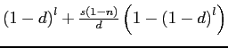
Starting again with the Calvo model with uncorrelated exchange rate innovations, we have
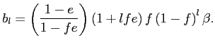
|
(6) |
The size of the bias depends on the relative strength of two
opposite forces. On the one hand, selective exits censor price
adjustments, thus dampening the response of the price index to past
exchange rate movements. This force is represented by the term
![]() ,
which we encountered earlier. On the other hand, exits also create
opportunities to introduce items whose price has not changed for
some time. This possibility subsequently makes the price level more
responsive to past exchange rate movements. This second force is
captured by
,
which we encountered earlier. On the other hand, exits also create
opportunities to introduce items whose price has not changed for
some time. This possibility subsequently makes the price level more
responsive to past exchange rate movements. This second force is
captured by ![]() . For short lags, the downward bias
is the predominant force. In particular, the initial response of
the index,
. For short lags, the downward bias
is the predominant force. In particular, the initial response of
the index,
![]() , is always downwardly
biased. As we increase the number of lags,
, is always downwardly
biased. As we increase the number of lags,
![]() grows linearly to any
arbitrarily large number, so that individual coefficients are
systematically upwardly biased at sufficiently long lags.
Nevertheless, the cumulative index response remains downwardly
biased because the coefficients converge more rapidly to
zero.17
grows linearly to any
arbitrarily large number, so that individual coefficients are
systematically upwardly biased at sufficiently long lags.
Nevertheless, the cumulative index response remains downwardly
biased because the coefficients converge more rapidly to
zero.17
As shown in the left panels of figure 3, assuming
that exiting items are replaced by sampling at random from the
population (![]() ) reduces the size of the bias
noticeably over the forecast horizon in the Calvo model relative to
the case in which entries are selective (
) reduces the size of the bias
noticeably over the forecast horizon in the Calvo model relative to
the case in which entries are selective (![]() ). For
frequencies of about 20 percent, the estimated two-year cumulative
response is nearly the same as the true one. The randomization of
entries mitigates the bias from selective exits because some of the
entering items have not had a price change in a while, making them
responsive to past exchange rate movements. As our figure
illustrates, this counterbalancing effect can be quite large,
offsetting much of the bias by the end of typical forecast
horizons.
). For
frequencies of about 20 percent, the estimated two-year cumulative
response is nearly the same as the true one. The randomization of
entries mitigates the bias from selective exits because some of the
entering items have not had a price change in a while, making them
responsive to past exchange rate movements. As our figure
illustrates, this counterbalancing effect can be quite large,
offsetting much of the bias by the end of typical forecast
horizons.
The gains from resampling at random are more modest in the
menu-cost model (right panels) because pass-through is very rapid.
As hinted in equation 6, the
counterbalancing effect of random substitutions grows with the
number of lags, ![]() , but since coefficients are tiny
after a small number of lags in the menu-cost model, the ultimate
impact on cumulative pass-through is modest.
, but since coefficients are tiny
after a small number of lags in the menu-cost model, the ultimate
impact on cumulative pass-through is modest.
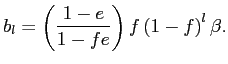
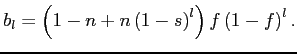
3.4 All Exits are Random and all Entries are Selective
We next turn our attention to the case in which all exits are
random and all entries are selective (![]() and
and
![]() ). Under these assumptions, the (plim)
coefficient on the
). Under these assumptions, the (plim)
coefficient on the ![]() lag of exchange
innovations in our baseline Calvo model is
lag of exchange
innovations in our baseline Calvo model is
| (7) |
This expression has a very intuitive interpretation. For a movement
in the exchange rate ![]() periods ago to contribute
to inflation in the current period, one must observe a price change
in the current period (probability
periods ago to contribute
to inflation in the current period, one must observe a price change
in the current period (probability ![]() ) and no
price change or substitution in the previous
) and no
price change or substitution in the previous ![]() periods (constant probability
periods (constant probability ![]() and
and ![]() , respectively, each period). Price changes and
substitutions from period
, respectively, each period). Price changes and
substitutions from period ![]() to
to ![]() result in posted prices that already reflect movements in
the exchange rate at period
result in posted prices that already reflect movements in
the exchange rate at period ![]() . Relative to
equation 2, the above
expression is downwardly biased by a factor
. Relative to
equation 2, the above
expression is downwardly biased by a factor
![]() .
.
A few comments are worth making. First, the nature of the
product replacement bias is that items entering the basket
systematically are less sensitive to past movements in the
exchange rate than items in general. Including entering items in
pass-through regressions thus lowers estimated pass-through rates.
Second, in the special case of ![]() , we have
, we have
![]() ; the estimated initial impact
of an exchange rate movement on the price index is always unbiased.
We also note that the share of the true coefficient correctly
measured decays exponentially with the number of lags considered.
The importance of the bias as a share of the cumulative response
thus grows over time, with estimates of the short-run cumulative
response being less biased than estimates of the long-run
response.
; the estimated initial impact
of an exchange rate movement on the price index is always unbiased.
We also note that the share of the true coefficient correctly
measured decays exponentially with the number of lags considered.
The importance of the bias as a share of the cumulative response
thus grows over time, with estimates of the short-run cumulative
response being less biased than estimates of the long-run
response.
Third, as stressed by Nakamura and Steinsson (2011), the bias is
most important for product categories with very low frequency of
price changes. The left panels of figure 4 illustrate the bias over the policy-relevant horizon under Calvo
pricing by plotting the cumulative contribution of the
coefficients. As seen in the figure, the bias increases in severity
with the degree of price stickiness. Only two thirds of the actual
cumulative pass-through is correctly estimated at a two-year
horizon when the frequency of price changes is 5
percent, and almost one fifth is still missing when the frequency
is 20 percent. For a frequency of 35 percent, the econometrician captures more than 95 percent of the true response over the forecast horizon.
Under Calvo pricing, only
![]() of the contribution
of lag
of the contribution
of lag ![]() to pass-through is correctly estimated.
This term typically is decreasing at a slow rate since
to pass-through is correctly estimated.
This term typically is decreasing at a slow rate since ![]() is small in practice, meaning that the product replacement
bias kicks in most strongly when much of the exchange rate response
occurs at long lags. Under low frequencies of price changes, the
coefficients associated with long lags in the Calvo model account
for a substantial share of the long-run price response, so that the
product replacement bias can become large over long horizons.
is small in practice, meaning that the product replacement
bias kicks in most strongly when much of the exchange rate response
occurs at long lags. Under low frequencies of price changes, the
coefficients associated with long lags in the Calvo model account
for a substantial share of the long-run price response, so that the
product replacement bias can become large over long horizons.
More generally, the size of the bias appears to be related to the speed at which the price index responds to an exchange rate shock. The right panels of figure 4 show the estimated cumulative contribution of the regression coefficients on the various lags of exchange rate movements (the dark-shaded bars), along with the bias left out by the econometrician (the light-shaded bars), under menu-cost pricing. The bias is much less severe than under Calvo pricing. Even for frequencies of price changes as low as 5 percent (upper-left panel), the econometrician captures almost 90 percent of the price index response at the two-year horizon. In the menu-cost model, most of the long-run pass-through occurs in the first few periods following a shock - even at low frequencies - so that the bias does not have time to cumulate to something large.
Finally, our figure depicts the worst-case assumption that all
entries are selective (![]() ). As noted in section 3.1, there would be
no bias if price collectors were replacing exiting items by
observations randomly selected from the population (
). As noted in section 3.1, there would be
no bias if price collectors were replacing exiting items by
observations randomly selected from the population (![]() ). In the more general case where all exits are random and
a fraction
). In the more general case where all exits are random and
a fraction ![]() of entries are selective, for the
Calvo model, we have
of entries are selective, for the
Calvo model, we have
Given this expression, we have that long-run pass-through is
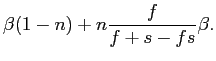
Departing from the extreme case of ![]() can
substantially reduce the size of the bias. As a rule of thumb, the
reduction in the bias by the end of the forecast horizon is roughly
proportional to
can
substantially reduce the size of the bias. As a rule of thumb, the
reduction in the bias by the end of the forecast horizon is roughly
proportional to ![]() , so that, for example, setting
, so that, for example, setting
![]() would roughly halve the area
represented by the light bars.
would roughly halve the area
represented by the light bars.
3.5 Comparing our Four Canonical Cases with Product Replacement Bias
Having laid out these four canonical cases, we can now compare
our findings with the product replacement bias discussed in
Nakamura and Steinsson (2011). Under the assumption of Calvo price
setting, if all entries are selective
![]() , then, for both the
selective exit-selective entry case and the random exit-selective
entry case, the long-run pass-through expressions can be written as
, then, for both the
selective exit-selective entry case and the random exit-selective
entry case, the long-run pass-through expressions can be written as
 , where
![]() is the observed frequency of price
changes. This implied correction factor is the same as the one
reported in Nakamura and Steinsson (2011).18 This long-run
pass through expression holds whenever all entries are selective
is the observed frequency of price
changes. This implied correction factor is the same as the one
reported in Nakamura and Steinsson (2011).18 This long-run
pass through expression holds whenever all entries are selective
![]() as one can write the
regression coefficients as
as one can write the
regression coefficients as
The above result that a single expression captures the bias whether exits are selective or random is not a general one, however. As we will now argue, it does not hold (a) when one departs from the knife-edge case in which all entries are selective, (b) when one is interested in correcting the dynamics, or (c) under other models than Calvo.
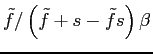
Departure from the assumption that all entries are selective.
Whenever some entries are random (![]() ), the
long-run pass-through correction factor depends on whether exits
are random or selective. To see this, suppose, that all entries are
random
), the
long-run pass-through correction factor depends on whether exits
are random or selective. To see this, suppose, that all entries are
random
![]() . If all exits are also
random, then the coefficients
. If all exits are also
random, then the coefficients ![]() can be
expressed as
can be
expressed as
 . In contrast, if
all exits are selective, then the coefficients are
. In contrast, if
all exits are selective, then the coefficients are
The corresponding long-run pass-through corrections are not the same in these two cases. In particular, as we showed above, the long-run correction factor is 1 (i.e. no correction required) for random exit and random entry.
Dynamics.
Although one can correct long-run pass-through estimates using
only
![]() and
and ![]() when
when
![]() , it is not possible to do so over any
finite horizon in our environment without taking a stand on the
selectivity of exit. For example, the measured initial response
(i.e.,
, it is not possible to do so over any
finite horizon in our environment without taking a stand on the
selectivity of exit. For example, the measured initial response
(i.e., ![]() ) of the price level to a shock is
always
) of the price level to a shock is
always
![]() . Whether this is a biased
estimate of the true initial response depends on whether
. Whether this is a biased
estimate of the true initial response depends on whether
![]() correctly captures the true
frequency or not. The value of
correctly captures the true
frequency or not. The value of ![]() is the
true frequency when exits are random but not when exits are
selective. Thus,
is the
true frequency when exits are random but not when exits are
selective. Thus, ![]() is unbiased assuming random
exit and is biased assuming selective exit. Depending on one's
assumptions regarding exit, different correction factors are needed
at different horizons.
is unbiased assuming random
exit and is biased assuming selective exit. Depending on one's
assumptions regarding exit, different correction factors are needed
at different horizons.
Other pricing models.
Even when all entries are selective, the connection between long-run pass through in the random exit-selective entry case and the selective exit-selective entry case is specific to the Calvo model. As shown by our comparison of menu-cost and Calvo models, the speed of pass-through is quite important in determining the long-run effects when entry is selective. Models with similar observed frequencies can thus differ in terms of measured long-run pass through. In particular, holding constant the observed frequency, a menu-cost model with selective entry will have a small long-run bias when exits are random and entries are selective but a much larger bias when both exits and entries are selective.
3.6 Robustness to the Presence of Real Rigidities
Gopinath and Itskhoki (2011) find that movements in the exchange rate are passed-through to import prices over more than one price adjustment, consistent with the presence of real rigidities slowing the diffusion of the shock to reset prices. The model adopted so far abstracts from this possibility. However, we show in appendix B that the inclusion of real rigidities has a negligible impact on the theoretical correction factors one should apply to standard pass-through estimates. In particular, we prove that the correction factors for the initial and the long-run responses are independent of real rigidities in the Calvo model, and then show that the factors are overall insensitive to real rigidities at intermediate horizons.
Appendix B also shows that assuming the presence of real rigidities can alter one's judgment regarding the empirical relevance of the Calvo versus the menu-cost models. As we shall see shortly, the empirical impulse response of import prices to an exchange rate movement is consistent with features of both models, in particular the initially rapid response of the index predicted by the menu-cost model, and the continued pass-through over medium-term horizons predicted by the Calvo model. The assumption of real rigidities slows predicted pass-through, which makes it more challenging for the Calvo model to match the initial import price index response to an exchange rate movement.
4 Empirical Relevance of Selective Exits and Entries
In order to assess the impact of selective exits and selective
entries on standard estimates of exchange rate pass-through, one
needs to form a view on several objects that are not directly
observed, namely the type of price-setting frictions giving rise to
infrequent nominal adjustments, the extent of price change
censoring through exits (![]() ), and the prevalence of
entries whose prices are relatively unresponsive to past exchange
rate movements (
), and the prevalence of
entries whose prices are relatively unresponsive to past exchange
rate movements (![]() ). In this section, we first argue
that standard estimates of the import price response to exchange
rate movements mix features of both the menu-cost and the Calvo
models. We next simulate the models to derive bounds on the size of
the biases over our forecast horizon. Finally, we present an
alternative index construction method to purge standard
pass-through estimates of much of the product replacement bias.
). In this section, we first argue
that standard estimates of the import price response to exchange
rate movements mix features of both the menu-cost and the Calvo
models. We next simulate the models to derive bounds on the size of
the biases over our forecast horizon. Finally, we present an
alternative index construction method to purge standard
pass-through estimates of much of the product replacement bias.
4.1 Dynamic Transmission of Exchange Rate Shocks: Data Versus Models
We focus our empirical analysis on finished goods categories, which account for about 60 percent of the total value of U.S. imports. They comprise automotive products, consumer goods, and capital goods. We leave aside fuel and material-intensive goods because the problems associated with selective exits and selective entries appear relatively benign for those categories given that (i) they are relatively homogeneous products, (ii) they tend to be traded between a large number of buyers and sellers, and (iii) their prices can often be readily observed in electronic trading platforms. In fact, the IPP obtains its crude oil import prices from a source outside of the sampling universe we observe for this paper, which altogether precludes an empirical discussion of exit and entry in that important category. Finally, for an economy as large as the United States, exchange rate movements and the price of fuel and material-intensive categories are arguably simultaneously determined to some degree, which raises additional econometric issues.
Our estimation period begins in January 1994 and ends in March
2010. For each three-digit Enduse category (indexed by ![]() ), we construct a trade-weighted nominal exchange rate,
), we construct a trade-weighted nominal exchange rate,
![]() , and foreign producer price
inflation,
, and foreign producer price
inflation,
![]() . We then estimate by
ordinary least squares the following equation,
. We then estimate by
ordinary least squares the following equation,
The number of lags is greater than is typically used in empirical pass-through literature. However, given the simulation results reported earlier, the additional lags seem to be an appropriate choice for robustness. The estimated impulse responses to a 1-percent depreciation of the U.S. dollar are presented in figure 5. The largest responses are found for machinery and equipment categories (Enduse 210, 211, 212, and 215), and, especially, for computers and semi-conductors (Enduse 213). Incidentally, this last category is also one for which the BLS makes special efforts to hedonically adjust prices. By contrast, some categories show little if any pass-through over our two-year horizon, notably automobiles and other vehicles (Enduse 300 and 301), apparel (Enduse 400), and home entertainment equipment (Enduse 412).
To compute a response for finished goods, we aggregate our three-digit category responses using 2006 trade weights. As shown in the lower-left panel, finished goods prices climb more than 0.1 percentage point in the first two months following a 1-percent exchange rate depreciation, another 0.1 percentage point over the remainder the first year, and a more modest 0.05 percentage point over the course of the second year. We obtain a similar response when we regress the index for finished goods on the exchange rate (the dashed line in the lower-left panel).19 The shape of the impulse response shares aspects of both the menu-cost and Calvo models. The initially rapid response is qualitatively similar to that in the menu-cost model, whereas the ensuing slow but steady increase is more akin to the protracted response in the Calvo model.
Figure 6 directly compares the empirical responses in each three-digit Enduse category to those generated by the Calvo and menu-cost models. The models are calibrated to match category-level statistics as outlined in section 2.2, with the minor difference that we seek to match the observed cumulative rate of pass-though in the last quarter of the forecast horizon rather than some illustrative long-run value. Figure 6 also shows the linear combinations of model responses that minimize the Euclidian distance with the empirical response over the forecast horizon. Again, we find support for both models, with some Enduse categories clearly preferring one model over the other, and others being best represented by a mixture of the two models. On average, each model is attributed about half of the weight. Though the model responses displayed assume no selection effects, this finding is robust to assuming any degree of selective exits or selective entries in the calibration.
4.2 Bounding Standard Pass-Through Estimates
To assess the quantitative importance of selective exits and entries, our next strategy is to derive three sets of bounds on the amount of exchange rate pass-through over the policy horizon. These bounds are related to the canonical cases discussed in sections 3.2 to 3.3, depending on whether we consider, respectively, the largest plausible number of selective exits and entries consistent with the data, the largest plausible number of selective exits in the presence of random entries, or the largest plausible number of selective entries in the presence of random exits.
Our worst case of selective exits assumes that all out-of-scope
exits mask a price change. We treat exits for other reasons (as
defined in table 1) as random because they typically are planned
years in advance by the BLS and thus unlikely to be related to
individual pricing decisions. Under these assumptions, we observe
the rate of random exit, ![]() , and the rate of selective
exits,
, and the rate of selective
exits,
![]() , as they correspond to
the rate of out-of-scope and other exits shown in table 1.
Knowledge of these rates and of the observed frequency of price
changes,
, as they correspond to
the rate of out-of-scope and other exits shown in table 1.
Knowledge of these rates and of the observed frequency of price
changes,
![]() , is
sufficient to identify
, is
sufficient to identify ![]() ,
, ![]() , and
, and
![]() in the model. Our worst case of selective
entries occurs when all items added to the sample experience an
unobserved price change upon entry (i.e.,
in the model. Our worst case of selective
entries occurs when all items added to the sample experience an
unobserved price change upon entry (i.e., ![]() ).
).
Given the sensitivity of biases to price-setting assumptions, we
derive our bounds under both Calvo and menu costs. Under Calvo, we
compute the correction factors for the estimated cumulative
response to an exchange rate movement directly from the analytical
expressions for the estimated coefficients, shown in equations 5 to 7. Under menu
costs, no such expressions are available, so we compute the
corresponding correction factors through simulations. In
particular, for each three-digit Enduse category, we select
![]() ,
, ![]() ,
and
,
and ![]() to match the observed frequency of
price changes, the average absolute size of price changes, and the
cumulative amount of pass-through by the last quarter of the
forecast horizon following a 1-percent depreciation of the dollar.
We then apply the correction factors to the estimated responses and
aggregate them using 2006 trade shares to derive our bounds on the
response of finished goods.
to match the observed frequency of
price changes, the average absolute size of price changes, and the
cumulative amount of pass-through by the last quarter of the
forecast horizon following a 1-percent depreciation of the dollar.
We then apply the correction factors to the estimated responses and
aggregate them using 2006 trade shares to derive our bounds on the
response of finished goods.
Our worst case of selective exits and entries is shown in the upper-left panel of figure 7. The estimated finished goods price response to a 1-percent depreciation of the dollar is 0.24 percent by the last quarter of the forecast horizon. After correcting for selective exits and selective entries, this figure could be as large as 0.30 percent in the menu-cost model, and 0.32 percent in the Calvo model. The slightly wider bound under Calvo pricing is due to the larger correction for selective entries in that model. If we instead assume that all entries are random (upper-right panel), then the corrected estimate in the last quarter falls to at most 0.26 percent under Calvo, and to at most 0.28 percent under menu costs. The bias is larger under menu costs in this case because the benefits from randomizing entries are largest when pass-through is slow, as in the Calvo model.20Under the worst case of product replacement bias (lower-left panel), the corrected response is very close to the actual response under menu costs, but remains somewhat higher (0.30 percent) than the uncorrected estimate (0.24 percent) by the last quarter of the forecast horizon. Even in this case, the near-term estimate remains relatively precise, however.
Given our earlier evidence that features of both models are present in the data, we derive a fourth set of bounds under what we view as more plausible price-setting assumptions. The three-digit Enduse responses of the Calvo and menu-cost models are first weighted according to the linear combination that provides the best fit of the empirical response, as we did in the previous section, and then aggregated using 2006 trade shares. We posit that all out-of-scope exits correspond to selective exits and selective entries, whereas all other exits are associated with random exits and random entries, so that about half of all exits and entries are selective. The corrected cumulative response under this last set of assumptions is presented in the lower-right panel of figure 7. Following a 1-percent depreciation of the dollar, the corrected cumulative response by the last quarter (0.28 percent) is above the estimated one (0.24 percent). Selective exits and selective entries contribute roughly equally to this difference, as hinted by the special case with only selective entries that is also displayed in the panel.
Summing up, our bound analysis suggests that, even under the stringent assumptions consistent with the microdata, the biases induced by selective exits and selective entries have a limited impact on standard pass-through estimates for finished goods over typical forecast horizons. Given that this conclusion contrasts, at least on the surface, with Nakamura and Steinsson's (2011) assertion that the product replacement bias is quantitatively important, we next discuss how our respective findings can be reconciled.
4.3 Reconciling our Results with Those of Nakamura and Steinsson (2011)
We highlight four differences between our treatment of the product replacement bias and that of Nakamura and Steinsson (2011): the price index of interest, the time horizon of interest, the assumed distribution of heterogeneity in price-setting decisions, and the incidence of selective entries. To facilitate comparisons, we begin by estimating an equation for empirical pass-through that is very similar to equation 1 in their paper,
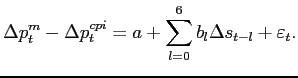
|
(8) |
We regress the difference between changes in the log of quarterly
import prices excluding oil,
![]() , and changes in the log of
U.S. CPI excluding food and energy,
, and changes in the log of
U.S. CPI excluding food and energy,
![]() , on a constant as well
as the contemporaneous and first
, on a constant as well
as the contemporaneous and first ![]() lags of the change
in log of the Federal Reserve's trade-weighted major currencies
real exchange rate index,
lags of the change
in log of the Federal Reserve's trade-weighted major currencies
real exchange rate index,
![]() . Our estimation period is
from 1995:Q1 to 2010:Q4 and the import price index is the deflator
from the National Economic Accounts from the U.S. Bureau of
Economic Analysis.
. Our estimation period is
from 1995:Q1 to 2010:Q4 and the import price index is the deflator
from the National Economic Accounts from the U.S. Bureau of
Economic Analysis.
As table 2 shows, our estimated import price response after 6 quarters is 0.41, a figure nearly identical to that reported by Nakamura and Steinsson (0.43). Any substantive difference between our findings below and those of Nakamura and Steinsson (2011) will thus be unrelated to our respective standard pass-through estimates. Table 2 also presents standard pass-through estimates after 6 quarters for two special groups of products, namely finished goods (Enduse categories in the 200s, 300s, and 400s) and material-intensive goods excluding oil (Enduse categories below 200, excluding 100). The rate of pass-through after 6 quarters is much lower for finished goods prices (0.26) than it is for material-intensive goods prices (0.93), highlighting the two groups' sharply different medium-term responses to exchange rate movements. The high pass-through estimate for material-intensive goods is perhaps not surprising given these items' frequent price adjustments, their high commodity content, and the strong relationship between commodity prices and the exchange rate. With pass-through nearly complete after 6 quarters, it is unlikely these items are plagued by severe product replacement biases, further justifying our focus on finished goods in earlier sections.21
To facilitate comparison to Nakamura and Steinsson's results, we
momentarily assume that the rate of substitution, ![]() ,
and the true pass-through coefficients,
,
and the true pass-through coefficients, ![]() , are the
same for all items in the IPP sample, leaving only the frequency of
price changes free to vary across items. The assumption of
identical pass-through rates across items in the sample is
admittedly unappealing given the evidence presented above for
finished goods and material-intensive goods, but it makes the
comparison to Nakamura and Steinsson (2011) more direct. The
monthly rate of substitution is set to 2.5 percent, a
figure in the range of rates reported in table 1.22 For
now, we maintain our assumption that items within each 3-digit
Enduse categories share the same frequency of price changes (these
frequencies are reported in table 1). In addition, to facilitate
further comparison with Nakamura and Steinsson's (2011) results, we
will calculate the bias-correction factors under the assumption
that the data are generated by a Calvo pricing model and that all
entries are selective.23
, are the
same for all items in the IPP sample, leaving only the frequency of
price changes free to vary across items. The assumption of
identical pass-through rates across items in the sample is
admittedly unappealing given the evidence presented above for
finished goods and material-intensive goods, but it makes the
comparison to Nakamura and Steinsson (2011) more direct. The
monthly rate of substitution is set to 2.5 percent, a
figure in the range of rates reported in table 1.22 For
now, we maintain our assumption that items within each 3-digit
Enduse categories share the same frequency of price changes (these
frequencies are reported in table 1). In addition, to facilitate
further comparison with Nakamura and Steinsson's (2011) results, we
will calculate the bias-correction factors under the assumption
that the data are generated by a Calvo pricing model and that all
entries are selective.23
As in Nakamura and Steinsson (2011), we obtain corrected
pass-through estimates by applying a correction factor, ![]() , to the sum of estimated coefficients after 6
quarters,
, to the sum of estimated coefficients after 6
quarters,
|
(9) |
For long-run pass-through, the correction factor is the following,
![]() is the factor
we would apply to standard pass-through estimates if our forecast
horizon was infinite, an approach close in spirit to that of
Nakamura and Steinsson (2011).24 The term
is the factor
we would apply to standard pass-through estimates if our forecast
horizon was infinite, an approach close in spirit to that of
Nakamura and Steinsson (2011).24 The term
 is the share
of long-run pass-through correctly estimated in product category
is the share
of long-run pass-through correctly estimated in product category
![]() , where
, where ![]() is the
observed frequency of price changes. Under the assumption of random
exit, the observed rate equals the true rate
is the
observed frequency of price changes. Under the assumption of random
exit, the observed rate equals the true rate ![]() ,
whereas under the assumption of selective exit, the observed rate
is less than the true rate
,
whereas under the assumption of selective exit, the observed rate
is less than the true rate ![]() .
.
In addition, we report correction factors for the cumulated response of the index 6 quarters (i.e., 18 months) after an exchange rate movement. As mentioned earlier, the dynamics of pass-through depend on the assumptions regarding entry. Under the assumption of random exit and selective entry.
The expression in the weighted sum represents the share of true
pass-through correctly estimated after 6 quarters in
3-digit Enduse category ![]() . It is obtained by dividing
the sum over the first 18 months of the biased coefficients (shown
in equation 7) by the
corresponding sum of the unbiased coefficients (shown in equation 4).
. It is obtained by dividing
the sum over the first 18 months of the biased coefficients (shown
in equation 7) by the
corresponding sum of the unbiased coefficients (shown in equation 4).
![]() roughly equals the correction factor we would apply to standard
pass-through estimates near the end of our two-year horizon. Note
that, under the assumption of random exit and selective entry, the
correction of the initial response,
roughly equals the correction factor we would apply to standard
pass-through estimates near the end of our two-year horizon. Note
that, under the assumption of random exit and selective entry, the
correction of the initial response,
![]() ,
equals one. By contrast, under the assumption of selective exit and
selective entry, the correction factor at any horizon is the same
as
,
equals one. By contrast, under the assumption of selective exit and
selective entry, the correction factor at any horizon is the same
as
![]() given above.
given above.
Under the assumption of random exit, the choice of either
![]() or
or
![]() as the
correction factor makes a noticeable difference on the resulting
corrected pass-through estimates. Our standard estimate for
imported goods excluding oil (0.41) rises to
0.47 when we use
as the
correction factor makes a noticeable difference on the resulting
corrected pass-through estimates. Our standard estimate for
imported goods excluding oil (0.41) rises to
0.47 when we use
![]() ,
and to
,
and to ![]() when we use
when we use
![]() . According to
these estimates, the bias in the long-run response is roughly twice
as large as the bias in the response after 6 quarters, showing that
much of the product replacement bias on long-run estimates falls
outside of typical policy horizons. Hence, one important difference
between our results and those of Nakamura and Steinsson (2011) is
that we use correction factors consistent with different time
horizons under the assumption of random entry.
. According to
these estimates, the bias in the long-run response is roughly twice
as large as the bias in the response after 6 quarters, showing that
much of the product replacement bias on long-run estimates falls
outside of typical policy horizons. Hence, one important difference
between our results and those of Nakamura and Steinsson (2011) is
that we use correction factors consistent with different time
horizons under the assumption of random entry.
We note that the correction factors for finished goods after six quarters (1.19) and over the long run (1.40) are noticeably larger than for material intensive goods over these horizons (1.10 and 1.13, respectively). The need for a larger correction for finished goods reflects their relatively slow pass-through of exchange rate shocks. In the case of material-intensive goods, the corrected estimates after 6 quarters (1.02) and over the long run (1.04) imply that true pass-through is complete over typical policy horizons.25
Another important difference between our results and those of
Nakamura and Steinsson is the treatment of heterogeneity in the
frequency of price changes across items. Throughout our paper, we
assume that the frequency of price changes is constant within
3-digit Enduse categories, otherwise leaving the frequency free to
vary across sectors of activity. This approach may leave some
heterogeneity unaccounted for within 3-digit Enduse categories,
which would lead us to underestimate the importance of the product
replacement bias. By contrast, Nakamura and Steinsson (2011)
control for the heterogeneity across firms by assuming that the
frequency of price changes is distributed according to a Beta
distribution, estimated on observed frequencies. When we adopt
their parametrization of the Beta distribution (using ![]() and
and ![]() as parameters), our corrected
long-run pass-through estimate for imported goods leaps from
0.52 to 0.70, a number in
the same range as the one they report (0.67). This
large correction is driven by a mass of observations at very low
frequencies of price changes. One salient feature of the Beta
distribution estimated by Nakamura and Steinsson (2011) is the
implication that a third of all observations have a monthly
frequency below 2 percent (i.e., with an average duration between
price adjustments greater than 4 years), with the density of
observations becoming arbitrarily large as the frequency approaches
zero. Or, the long-run correction factor is quite sensitive to the
presence of very low frequencies because
as parameters), our corrected
long-run pass-through estimate for imported goods leaps from
0.52 to 0.70, a number in
the same range as the one they report (0.67). This
large correction is driven by a mass of observations at very low
frequencies of price changes. One salient feature of the Beta
distribution estimated by Nakamura and Steinsson (2011) is the
implication that a third of all observations have a monthly
frequency below 2 percent (i.e., with an average duration between
price adjustments greater than 4 years), with the density of
observations becoming arbitrarily large as the frequency approaches
zero. Or, the long-run correction factor is quite sensitive to the
presence of very low frequencies because
![]() converges to zero as
converges to zero as
![]() approaches zero, making the correction
factor arbitrarily large.
approaches zero, making the correction
factor arbitrarily large.
To illustrate the sensitivity of the estimated long-run response to the mass of firms updating prices very infrequently, we move all observations with a frequency below 2 percent to a mass point at 2 percent. The correction factor for the long-run response falls from 1.70 to 1.47. This decline in the correction factor should caution us against driving strong conclusions that depend on the very low frequencies of price changes, whose density is difficult to estimate. In particular, the Beta distribution has only two parameters to capture the whole range of variation in the density of frequencies in the sample. It is thus conceivable that some of the very low frequencies implied by the calibration are off the empirical support.
Furthermore, as noted earlier, a severely biased long-run response need not imply a severely biased medium-term response. Under the assumption of random exit, much of the product replacement bias accrues beyond typical policy horizons. In the case of Nakamura and Steinsson's Beta distribution, the correction factor for the 6-quarter response under the assumption of random exit is only 1.17, a number well below that for the long-run response (1.70).
We conclude our comparison by stressing that we see the
correction factors derived above as worst cases rather than as base
cases. As argued in section 1,
we find limited evidence that the BLS methodology is conducive to
systematically adding items recently repriced to the IPP sample.
The correction factors shrink greatly as we lower the value of
![]() the fraction of entries that are
selective. The general formula for the correction factor is
the fraction of entries that are
selective. The general formula for the correction factor is
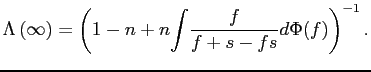
Therefore, if 50 percent of all entries have zero
price pressure (i.e. ![]() , a figure in line with
all forced exits being associated with a selective entry), then the
correction factor is only 1.26 under Nakamura
and Steinsson's Beta distribution. We also note that our impulse
response analysis in section 4.1 suggests that
pass-through is faster than implied by Calvo pricing for several
Enduse categories, consistent with lower correction factors than
derived above whenever some exits are random.
, a figure in line with
all forced exits being associated with a selective entry), then the
correction factor is only 1.26 under Nakamura
and Steinsson's Beta distribution. We also note that our impulse
response analysis in section 4.1 suggests that
pass-through is faster than implied by Calvo pricing for several
Enduse categories, consistent with lower correction factors than
derived above whenever some exits are random.
4.4 Reducing Biases Through Delayed Entries
If the estimates were subject solely to a product replacement
bias, then one could use a simple trick to remove much of that bias
over the policy-relevant horizon. Recall that the product
replacement bias arises because entering items systematically are
less responsive to past exchange rate movements than items in the
universe. Therefore, simply delaying the entry of substitutes into
the index should reduce this bias. We show in the appendix that,
when all exits are random and all entries are selective, the
estimated (plim) coefficients in a Calvo model with an arbitrary
![]() -period entry delay are given by
-period entry delay are given by
![\begin{displaymath} b_{l}=\left \{ \begin{array}[c]{cc} f\left( 1-f\right) ^{l}\beta & \text{if }l\leq M\ \left( 1-s\right) ^{l-M}f\left( 1-f\right) ^{l}\beta & \text{if }l>M \end{array}\right. . \end{displaymath}](img269.gif)
Delaying entries thus eliminates the product replacement bias for
the coefficients associated with the first ![]() lags of
exchange rate movements. The bias on subsequent lags is also
reduced, with
lags of
exchange rate movements. The bias on subsequent lags is also
reduced, with ![]() representing a fraction
representing a fraction
![]() of the true
response when entries are delayed by
of the true
response when entries are delayed by ![]() periods,
compared to only
periods,
compared to only
![]() when there is no
entry delay.
when there is no
entry delay.
The left panels of figure 8 show that delaying entries by 6 months can go a long way in reducing the product replacement bias over the policy-relevant horizon in the Calvo model. The bias at the end of the horizon is negligible when prices are adjusted 20 percent of the time or more. Even at frequencies as low as 5 percent, the prediction over the first year of the forecast suffers little product replacement bias, while the accuracy of the response in the second year is greatly improved. The bias reduction is even larger in the menu-cost model (right panels). Delaying entries by 6 months virtually eliminates the product replacement bias at all frequencies considered. The consistency gains are especially large in the menu-cost model because delaying entries corrects most effectively biases associated with short lags of the exchange rate, which account for the bulk of the price level response.
It turns out that our trick of delaying entries can also
mitigate biases in the presence of selective exits. We show in the
appendix that, with both selective exits and selective entries that
the (plim) regression coefficients under an ![]() -period
entry delay in the Calvo model are
-period
entry delay in the Calvo model are
![\begin{displaymath} b_{l}\left( M\right) =\left \{ \begin{array}[c]{cc} \frac{\left( 1-e\right) }{\left( 1-fe\right) ^{l+1}}f\left( 1-f\right) ^{l}\beta & \text{if }l\leq M\ \frac{\left( 1-e\right) }{\left( 1-fe\right) ^{M+1}}\left( \left( 1-d\right) ^{l-M}+\frac{s\left( 1-n\right) }{d}\left( 1-\left( 1-d\right) ^{l-M}\right) \right) f\left( 1-f\right) ^{l}\beta & \text{if }l>M \end{array}\right. . \end{displaymath}](img280.gif)
We also prove that the bias diminishes as one increases the entry delay given any forecast horizon. As one delays entries by an arbitrary large number of periods, we have
In short, the estimated long-run pass-through in the Calvo model is unbiased in the limit, a result that holds whether exits are selective, entries are selective, or both. The short-run response remains downward biased in the presence of selective exit, however.
The intuition for why delaying entries can improve pass-through
estimates in the presence of selective exits is somewhat subtle.
Remember that, for a movement in the exchange rate ![]() periods ago to have an impact on the index today, there must have
been no price change over the past
periods ago to have an impact on the index today, there must have
been no price change over the past ![]() periods.
Delaying entries by
periods.
Delaying entries by ![]() periods eliminates
observations incorporated into the index in recent periods, leaving
only those present in the index for at least
periods eliminates
observations incorporated into the index in recent periods, leaving
only those present in the index for at least ![]() periods. Or, these surviving observations are less likely than
observations in the universe to have experienced a price change
over the past
periods. Or, these surviving observations are less likely than
observations in the universe to have experienced a price change
over the past ![]() period (since observations with a
price change are more likely to have exited), meaning that they are
relatively more likely to contribute to inflation today. Under
Calvo pricing (left panels of figure 9), it
turns out that this selection effect perfectly offsets the downward
bias stemming from the censoring of price changes as we consider an
arbitrary long entry delay and forecast horizon. Under menu-cost
pricing (right panels), the gains are negligible due to the greater
mixing of observations.
period (since observations with a
price change are more likely to have exited), meaning that they are
relatively more likely to contribute to inflation today. Under
Calvo pricing (left panels of figure 9), it
turns out that this selection effect perfectly offsets the downward
bias stemming from the censoring of price changes as we consider an
arbitrary long entry delay and forecast horizon. Under menu-cost
pricing (right panels), the gains are negligible due to the greater
mixing of observations.
Our simulations suggest that delaying entries is most effective at reducing biases associated with selective entries over typical forecast horizons, a finding that is robust across pricing mechanisms and degrees of price flexibility. Thus, delaying entries can help us shed light on the empirical importance of selective entries: If estimated pass-through over the forecast horizon increases much after delaying entries, then selective entries may be economically important. By contrast, if estimated pass-through is insensitive to delaying entries, then selective entries may be a marginal phenomenon.
Using the BLS microdata, we have computed price indexes for the Enduse categories belonging to capital goods, automotive products, and consumer goods. We have constructed one index using the methodology introduced in section 1 (i.e., there is no entry delay and missing prices are carried forward). We have also constructed two alternative indexes that implement a 6-month and a 9-month entry delay, respectively. Figure 10 displays the results. As the left-hand column shows, these alternative price indexes are somewhat more volatile than the corresponding published BLS index (the thick black line), especially when entry is delayed. However, estimated pass-through rates are very similar whether we use the published BLS index or our constructed indexes. If selective entry were quantitatively important, then the estimated pass-through rates for the constructed indexes with delayed entry should be noticeably greater than the pass-through rates for the published index or for the constructed index with no delay. Instead, the estimated pass-through rates are very similar. Thus, the available evidence suggests a limited role for selective entry.
5 Concluding Remarks
We have investigated selection biases in standard exchange rate pass-through regressions that arise from missing price changes either due to item exit from or entry into the index. For both Calvo and menu-cost price-setting models, we have shown that these selection effects lower the measured response of an import price index to exchange rate movements over typical policy horizons and that the magnitude of the biases can be sensitive to price-setting assumptions.
In particular, in the presence of both selective exits and selective entries, the import price response is biased downward in both models. Assuming that entering items are sampled randomly from the universe alleviates some of the bias, especially under Calvo pricing. When entries are selective and exits occur at random, the downward bias tends to be small in the menu-cost model over any horizon, whereas the bias slowly grows from being negligible at short horizons to quite large over extended horizons in the Calvo model.
Assessing the quantitative importance of the biases is inherently challenging because selective exits and selective entries are, by their very nature, not observed. Our review of the BLS methodology suggests a moderate risk of such selection effects taking place in practice. We also argue that, under plausible assumptions about nominal price stickiness and the incidence of selective exits and selective entries, the presence of downward biases in standard pass-through regressions, although a concern, does not materially alter the literature's view that pass-through to U.S. import prices is low over typical forecast horizons. Even under our worst-case scenario, our estimated empirical bounds imply that at most about a third of an exchange rate shock is passed through to the price of imported finished goods after two years. Furthermore, our worst-case scenario is likely too severe as our constructed alternative price indexes with delayed item entries suggest a limited role for selective entry.
Although we have focused on import prices, our findings are relevant to the study of any price index subject to selection effects in sample exit and sample entry. The implications of selective exits and selective entries also extend to the measurement of the response of price indexes to aggregate and idiosyncratic shocks other than exchange rate movements.
Future research should aim at better identifying the causes of item exits as well as the characteristics of added items. Currently, the information contained in the IPP database provides useful and suggestive, but ultimately limited, guidance on these aspects.
References
Atkeson, Andrew and Ariel Burstein (2008) "Pricing to Market, Trade Costs, and International Relative Prices," American Economic Review, vol. 98(5), pages 1998-2031.
Berger, David Berger, Jon Faust, John H. Rogers, and Kai Steverson (2009). "Border Prices and Retail Prices," International Finance Discussion Papers 972, Board of Governors of the Federal Reserve System.
Bergin, Paul, and Robert C. Feenstra (2009), "Pass-Through of Exchange Rates and Competition between Floaters and Fixers," Journal of Money, Credit and Banking, vol. 41, pages 35-70.
Bils, Mark (2009). "Do Higher Prices for New Goods Reflect Quality Growth or Inflation?," Quarterly Journal of Economics, Vol. 124(2), pages 637-675.
Bresnahan, Timothy F., and Robert J. Gordon (1997). "The Economics of New Goods," Studies in Income and Wealth, Volume 58, National Bureau of Economic Research.
Broda, Christian, and David E. Weinstein (2010). "Product Creation and Destruction: Evidence and Price Implications," American Economic Review, vol. 100(3), pages 691-723.
Bureau of Labor Statistics. "Handbook of Methods," Washington DC, April 1997.
Bureau of Labor Statistics. "Measurement Issues in the Consumer Price Index," Washington D.C., June 1997, http://www.bls.gov/cpi/cpigm697.htm (last access: March 2010)
Boskin, Michael J., E. Dulberger, R. Gordon, Z. Griliches, and D. Jorgenson (1996). "Toward a More Accurate Measure of the Cost of Living," Final Report to the Senate Finance Committee, December 4.
Campa, José Manuel and Linda S. Goldberg (2005). "Exchange Rate Pass-Through into Import Prices," Review of Economics and Statistics, vol. 87(4), pages 679-690.
Danziger, Leif (1999). "A Dynamic Economy with Costly Price Adjustments," American Economic Review, vol. 89(4), pages 878-901.
Gertler, Mark and John Leahy (2008). "A Phillips Curve with an Ss Foundation," Journal of Political Economy, vol. 116(3), pages 533-572.
Greenlees, John S., and Robert McClelland (2011). "Does Quality Adjustment Matter for Technologically Stable Products? An Application to the CPI for Food," American Economic Review, vol. 101(3), pages 200-205.
Goldberg, Pinelopi and Michael M. Knetter (1997). "Goods Prices and Exchange Rates: What Have We Learned?," Journal of Economic Literature, vol. 35(3), pages 1243-1272.
Gopinath, Gita and Oleg Itskhoki (2010). "Frequency of Price Adjustment and Pass-Through," Quarterly Journal of Economics, Vol. 125(2), pages 675-727.
Gopinath, Gita and Oleg Itskhoki (2011). "In Search of Real Rigidities," NBER Macroeconomics Annual, 2010, vol. 25, , pages 261-309.
Gopinath and Rigobon (2008), "Sticky Borders," Quarterly Journal of Economics, 123(2): 531-75.
Gopinath, Gita, Oleg Itskhoki, and Roberto Rigobon (2010). "Currency Choice and Exchange Rate Pass-Through," American Economic Review, vol. 100(1), pages 304-36.
Gordon, Robert J. (2006). "The Boskin Commission Report: A Retrospective One Decade Later," International Productivity Monitor, vol. 12, pages 7-22.
Gust, Christopher, Sylvain Leduc, and Robert J. Vigfusson (2010). "Trade Integration, Competition, and the Decline in Exchange-Rate Pass-Through," Journal of Monetary Economics, vol. 57(3), pages 309-324.
Marazzi, Mario, Nathan Sheets, Robert J. Vigfusson, Jon Faust, Joseph Gagnon, Jaime Marquez, Robert F. Martin, Trevor Reeve, John Rogers (2005). "Exchange Rate Pass-Through to U.S. Import Prices: Some New Evidence," International Finance Discussion Papers 833, Board of Governors of the Federal Reserve System.
Marazzi, Mario and Nathan Sheets (2007). "Declining Exchange Rate Pass-through to U.S. Import Prices: The Potential Role of Global Factors," Journal of International Money and Finance, vol. 26, pp. 924-47.
Nakamura, Emi, and Jón Steinsson (2011). "Lost in Transit: Product Replacement Bias and Pricing to Market," mimeo, Columbia University.
Neiman, Brent (2010). "Stickiness, Synchronization, and Passthrough in Intrafirm Trade Prices," Journal of Monetary Economics, April 2010.
Sheshinski, Eytan and Yoram Weiss (1977). "Inflation and Costs of Price Adjustment," Review of Economic Studies, vol. 44(2), pages 287-303.
A Regression Coefficients in the Calvo Model
In this appendix, we derive analytical expressions for pass-through coefficients when the data are generated by a Calvo model with selection biases in the exit and entry of items. The environment is as described in section 3 with the extra simplifying assumption that exchange rate innovations are uncorrelated over time. We begin by describing the general case. We then investigate how delaying the entry of items in the index affect the regression coefficients. We finally provide a proof that the bias on the coefficients declines as one delays the entry of items in the index.
A.1 General Case
Let
![]() ,
,
![]() , and
, and
![]() be indicator variables
that an item
be indicator variables
that an item ![]() present in the sample at the beginning
of period
present in the sample at the beginning
of period ![]() has experienced, respectively, a price
change, a random exit, and a selective exit (conditional on a price
change and no random exit). For any exiting item, we also define an
indicator variable
has experienced, respectively, a price
change, a random exit, and a selective exit (conditional on a price
change and no random exit). For any exiting item, we also define an
indicator variable
![]() that the corresponding
entry is selective. For convenience, let also
that the corresponding
entry is selective. For convenience, let also
![]() be an indicator variable that an item has exited during the
period, either through a random exit (probability
be an indicator variable that an item has exited during the
period, either through a random exit (probability ![]() )
or a selective exit (probability
)
or a selective exit (probability
![]() ).
).
We first derive an expression for the contemporaneous impact of an exchange rate movement on the price index. Using the covariance approach, we have
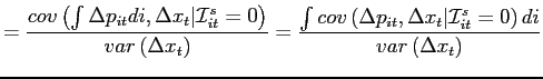
|
||
![$\displaystyle =\frac{cov(u_{it}+\beta \Delta x_{t}+\varepsilon_{it},\Delta x_{t} \vert\mathcal{I}_{it}^{s}=0,\mathcal{I}_{it}^{f}=1)}{var\left( \Delta x_{t}\right) }\Pr \left[ \mathcal{I}_{it}^{f}=1\vert\mathcal{I}_{it}^{s}=0\right]$](img298.gif)
|
||
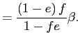 |
The covariance term is conditioned on
![]() because, among
observations present in the sample at the beginning of the period,
only those that do not exit can be used to compute inflation. These
usable observations either had no price change and no exit
(probability
because, among
observations present in the sample at the beginning of the period,
only those that do not exit can be used to compute inflation. These
usable observations either had no price change and no exit
(probability
![]() ) or a
price change and no exit (probability
) or a
price change and no exit (probability
![]() ). Only
the latter observations, which account for a share
). Only
the latter observations, which account for a share
![]() of
usable observations, can have a nonzero contribution to inflation.
of
usable observations, can have a nonzero contribution to inflation.
Proceeding similarly with ![]() ,
,
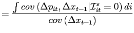
|
||
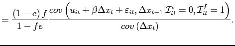
|
Since
![]() and
and
![]() are assumed to be
independent of
are assumed to be
independent of
![]() , the covariance term is
impacted solely through the possible interactions between
, the covariance term is
impacted solely through the possible interactions between
![]() and the cumulated price
pressure
and the cumulated price
pressure ![]() . Conditioning on past realizations of
the indicator variables, there are five distinct cases:
. Conditioning on past realizations of
the indicator variables, there are five distinct cases:
![$\displaystyle u_{it}=\left \{ \begin{array}[c]{cc} u_{it-1}+\beta \Delta x_{t-1}+\varepsilon_{it-1} & \text{if }\left \{ \mathcal{I}_{it-1}^{s}=0,\mathcal{I}_{it-1}^{f}=0\right \} \\ 0 & \text{if }\left \{ \mathcal{I}_{it-1}^{s}=0,\mathcal{I}_{it-1} ^{f}=1\right \} \\ u_{it-1}+\beta \Delta x_{t-1}+\varepsilon_{it-1} & \text{if }\left \{ \mathcal{I}_{it-1}^{s}=1,\mathcal{I}_{it-1}^{n}=0,\mathcal{I}_{it-1} ^{f}=0\right \} \\ 0 & \text{if }\left \{ \mathcal{I}_{it-1}^{s}=1,\mathcal{I}_{it-1} ^{n}=0,\mathcal{I}_{it-1}^{f}=1\right \} \\ 0 & \text{if }\left \{ \mathcal{I}_{it-1}^{s}=1,\mathcal{I}_{it-1} ^{n}=1\right \} \end{array} \right. .$](img313.gif)
|
(10) |
Consequently,
![$\displaystyle =\frac{\left( 1-e\right) f}{1-fe}\frac{cov\left( \beta \Delta x_{t-1},\Delta x_{t-1}\right) }{cov\left( \Delta x_{t}\right) }\left( \Pr \left[ \mathcal{I}_{it-1}^{s}=0,\mathcal{I}_{it-1}^{f}=0\right] +\Pr \left[ \mathcal{I}_{it-1}^{s}=1,\mathcal{I}_{it-1}^{n}=0,\mathcal{I} _{it-1}^{f}=0\right] \right)$](img315.gif)
|
||
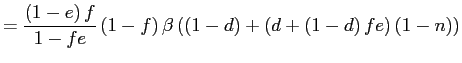
|
Intuitively, among all observations usable to compute inflation,
only those with a price change in the current period (marginal
probability
![]() ) and either
no price change and no exit in the previous period (marginal
probability
) and either
no price change and no exit in the previous period (marginal
probability
![]() ) or an
exit accompanied by no price change (marginal probability
) or an
exit accompanied by no price change (marginal probability
![]() ) have a nonzero contribution of
) have a nonzero contribution of
![]() to inflation.
to inflation.
The general case with ![]() is illustrated in the
upper panel of figure 11.
It shows the various states that are usable in the computation of
inflation at each period, along with their associated marginal
probability in each period. The arrows indicate the paths through
which an exchange rate movement in the period
is illustrated in the
upper panel of figure 11.
It shows the various states that are usable in the computation of
inflation at each period, along with their associated marginal
probability in each period. The arrows indicate the paths through
which an exchange rate movement in the period ![]() can be reflected as a nonzero price change in period
can be reflected as a nonzero price change in period
![]() . Observations that have not responded to
an exchange rate movement at period
. Observations that have not responded to
an exchange rate movement at period ![]() can find
their way in the index either by having been present in the sample
prior to period
can find
their way in the index either by having been present in the sample
prior to period ![]() or by entering the item through
a substitution. The marginal probability from period
or by entering the item through
a substitution. The marginal probability from period ![]() to period
to period ![]() associated with the
former event (no price change and no exit) is
associated with the
former event (no price change and no exit) is
![]() for
each period. The marginal probability associated with the addition
of an item in period
for
each period. The marginal probability associated with the addition
of an item in period ![]() whose last price change
was prior to period
whose last price change
was prior to period ![]() is the product of the
probability of having a substitution (probability
is the product of the
probability of having a substitution (probability
![]() ), a random selection
from the universe (probability
), a random selection
from the universe (probability ![]() ), and no price
change for
), and no price
change for ![]() periods (probability
periods (probability
![]() ). Summing up
across all usable paths, we have
). Summing up
across all usable paths, we have
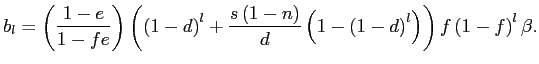
A.2 Delayed Entries
We next assume that the econometrician only uses observations
that have been in the sample for more than ![]() periods
in the computation of inflation. This assumption is made in section 4.4 to argue that
delaying the entry of items in the basket can mitigate some of the
biases associated with selective exits and entries. We distinguish
between two cases:
periods
in the computation of inflation. This assumption is made in section 4.4 to argue that
delaying the entry of items in the basket can mitigate some of the
biases associated with selective exits and entries. We distinguish
between two cases: ![]() and
and ![]() .
.
The first case is illustrated in the middle panel of figure 11. Because entries
are delayed by more periods than the lag of the exchange rate
movement considered, all observations used to compute inflation
have been continuously in the index since before period ![]() . For an exchange rate movement at period
. For an exchange rate movement at period ![]() to be reflected in a nonzero price change today, we must
have had had no price change from period
to be reflected in a nonzero price change today, we must
have had had no price change from period ![]() to
to
![]() (marginal probability
(marginal probability
![]() ), and
a price change at
), and
a price change at ![]() (marginal probability
(marginal probability
![]() ).
The resulting coefficient is
).
The resulting coefficient is
|
(11) |
The case of ![]() is illustrated at the bottom of
figure 11. It mixes
elements of the general case with no delay (upper panel) and the
case with
is illustrated at the bottom of
figure 11. It mixes
elements of the general case with no delay (upper panel) and the
case with ![]() (middle panel). Prior to period
(middle panel). Prior to period
![]() , observations that have not yet
responded to the exchange rate movement at period
, observations that have not yet
responded to the exchange rate movement at period ![]() could have found their way in the index either through a
substitution or by having been present in the sample before period
could have found their way in the index either through a
substitution or by having been present in the sample before period
![]() . From period
. From period ![]() onward,
only observations that are already present in the index at the end
of period
onward,
only observations that are already present in the index at the end
of period ![]() can be used to compute inflation.
Summing up the probabilities over all possible paths and
simplifying, we get
can be used to compute inflation.
Summing up the probabilities over all possible paths and
simplifying, we get

|
(12) |
A.3 Proof that Biases are Declining in the Entry Delay
We conclude this appendix by showing that delaying the entry of
items in the index always improves pass-though estimates. We assume
that the number of lags in the regression is at least as large as
the forecast horizon, ![]() , a condition typically
satisfied in standard pass-through regressions. Let
, a condition typically
satisfied in standard pass-through regressions. Let
![]() be the plim
coefficients associated with the
be the plim
coefficients associated with the ![]() -th lag of the
exchange rate and an entry delay of
-th lag of the
exchange rate and an entry delay of ![]() periods. The
proof proceeds in two steps. We first prove that
periods. The
proof proceeds in two steps. We first prove that
![]() , so that
delaying entries by an extra period always (weakly) increases the
size of the (plim) regression coefficients. We then show that the
cumulative response over any forecast horizon remains bounded above
by the true response.
, so that
delaying entries by an extra period always (weakly) increases the
size of the (plim) regression coefficients. We then show that the
cumulative response over any forecast horizon remains bounded above
by the true response.
A.3.1 Step 1:
We distinguish between three cases: ![]() ,
,
![]() , and
, and ![]() . When
. When
![]() , the plim coefficients are given by
equation 11, so that
, the plim coefficients are given by
equation 11, so that
![]() . When
. When
![]() ,
,
![]() is given by equation 12 and
is given by equation 12 and
![]() is given by
equation 11. For
is given by
equation 11. For
![]() to be
true in this case, we must have
to be
true in this case, we must have
Note that if the above equation holds for ![]() , then
it holds for all
, then
it holds for all
![]() . Imposing
. Imposing
![]() and using
and using
![]() , we have
, we have
which is always satisfied. Finally, we want to show that
![]() when
when
![]() . The plim coefficients are given by
equation 12. Note that
. The plim coefficients are given by
equation 12. Note that
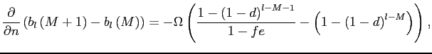
where ![]() is some positive constant. The
difference between
is some positive constant. The
difference between
![]() and
and
![]() is thus linear in
is thus linear in
![]() and either always increasing or always
decreasing in
and either always increasing or always
decreasing in ![]() . By showing that
. By showing that
![]() for
for
![]() and
and ![]() , we will prove
that the result holds for the worse scenario under either case.
Consider first
, we will prove
that the result holds for the worse scenario under either case.
Consider first
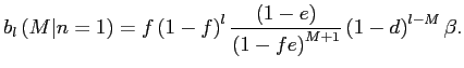
We have
![]() if and only if
if and only if
![]() , which is always true. Consider next
, which is always true. Consider next
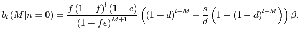
We have
![]() if and only if
if and only if

which can be shown to hold if and only if
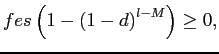
a condition that is always satisfied. Summing up, the individual coefficients are increasing in the entry delay, so that the cumulative pass-through over any forecast horizon also is increasing in the entry delay.
A.3.2 Step 2: Estimated Cumulative Response is Bounded Above by True Response
To complete the proof, we show that the estimated pass-through
under delayed entries never exceeds the true pass-through over any
forecast horizon. The true pass-through after ![]() periods is
periods is
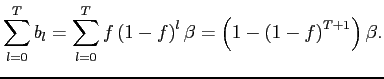
Because
![]() , the
estimated pass-through is largest when
, the
estimated pass-through is largest when ![]() which
is associated with
which
is associated with
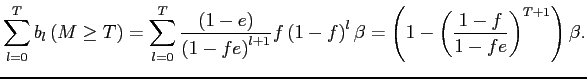
It is immediate that the above expression is bounded above by the unbiased case.
B Real Rigidities
To explore the incidence of real rigidities on our theoretical correction factors, we follow Gopinath and Itskhoki (2011) in adopting a flexible specification for the evolution of the firm's reset price,
The parameter
![]() controls the
extent of real rigidities by capturing the emphasis placed by the
firm on matching movements in the average price of competing
importers,
controls the
extent of real rigidities by capturing the emphasis placed by the
firm on matching movements in the average price of competing
importers,
![]() , when resetting its price. As
was the case earlier, a fraction
, when resetting its price. As
was the case earlier, a fraction ![]() of exchange
rate movements is passed-through to import prices in the long run.
of exchange
rate movements is passed-through to import prices in the long run.
Under Calvo pricing, it is possible to derive expressions for
the evolution of the true import price index and for the correction
factors in response to a one-time jump in the exchange rate.
Abstracting from idiosyncratic disturbances, which have no effect
on the index, the initial impact on reset prices is the sum of the
direct effect of
![]() on
on
![]() and of its indirect
effect through the change in the price of competing importers,
and of its indirect
effect through the change in the price of competing importers,
The impact in subsequent periods depends only on the evolution of the price of competing importers,
The price of competing importers evolves according to
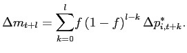
|
(13) |
Intuitively, the fraction ![]() of firms updating
their price in period
of firms updating
their price in period ![]() will take into account
will take into account
![]() in setting
in setting
![]() . Of these firms, a
fraction
. Of these firms, a
fraction ![]() did not update in period
did not update in period ![]() and will also take into account
and will also take into account
![]() . More generally, a
fraction
. More generally, a
fraction
![]() of firms updating in
period
of firms updating in
period ![]() will take into account
will take into account
![]() when setting
when setting
![]() .
.
The above three equations allow us to solve recursively for
![]() and
and
![]() . In the initial period,
. In the initial period,
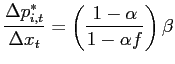
|
(14) |
and
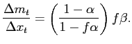
|
(15) |
Subsequently, one can show that
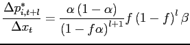
|
(16) |
and
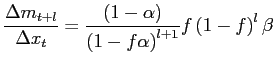
for ![]() . Absent real rigidities (
. Absent real rigidities (![]() ), the reset price would initially move by
), the reset price would initially move by
![]() and remain unchanged
thereafter. With real rigidities (
and remain unchanged
thereafter. With real rigidities (![]() ),
the reset price moves gradually toward its long-run level so that
the response to an exchange rate movement is spread over several
price adjustments. The cumulative response of the price of
competing importers after
),
the reset price moves gradually toward its long-run level so that
the response to an exchange rate movement is spread over several
price adjustments. The cumulative response of the price of
competing importers after ![]() period is given by
period is given by
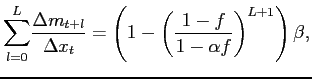
|
(17) |
which implies a slower rate of pass-through than the case with
![]() . The cumulative change in the
target price is a weighted sum of the long-run change and the
cumulative change in the price of competing importers,
. The cumulative change in the
target price is a weighted sum of the long-run change and the
cumulative change in the price of competing importers,
Using the arguments made in section 3 to derive equation (3), we can express the measured change in the import price index as
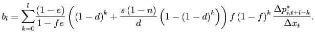
|
(18) |
The variable ![]() corresponds to the (plim)
regression coefficient on the
corresponds to the (plim)
regression coefficient on the ![]() -th lag of the
exchange rate. The above equation, along with equations (14) and
(16),
allow us to compute the
-th lag of the
exchange rate. The above equation, along with equations (14) and
(16),
allow us to compute the ![]() at all lags. To gain
intuition about the role of real rigidities, we shall highlight
three results.
at all lags. To gain
intuition about the role of real rigidities, we shall highlight
three results.
First, the correction factor on the initial response of the index is independent of the extent of real rigidities. This can be seen by using equations (14), (15), and (18) to write
The inverse of
![]() is
the correction factor applicable to the initial response. It does
not depend on
is
the correction factor applicable to the initial response. It does
not depend on ![]() . Second, the correction factor
for long-run pass-through is also independent of the extent of real
rigidities. This can be proven by considering the cumulative sum of
. Second, the correction factor
for long-run pass-through is also independent of the extent of real
rigidities. This can be proven by considering the cumulative sum of
![]() in equation (18) and taking its
limit as the horizon is extended. One can then show that
in equation (18) and taking its
limit as the horizon is extended. One can then show that
The inverse of the expression in front of ![]() is
the correction factor on long-run pass-through, which is again
independent of
is
the correction factor on long-run pass-through, which is again
independent of ![]() . Third, when both exits and
entries are selective, then the correction factors are independent
of real rigidities at all horizons. In such a case, a constant
fraction
. Third, when both exits and
entries are selective, then the correction factors are independent
of real rigidities at all horizons. In such a case, a constant
fraction
![]() of
of
![]() is missed every
period.
is missed every
period.
In the general case, the correction factors on the cumulative
index response may depend on ![]() at horizons
beyond the initial period but finite. However, we find that these
correction factors are rather insensitive to the extent of real
rigidities. This aspect is illustrated in figure 12 for a Calvo
model with a frequency of price changes of 15
percent and a rate of substitution of 5 percent. The
parameter
at horizons
beyond the initial period but finite. However, we find that these
correction factors are rather insensitive to the extent of real
rigidities. This aspect is illustrated in figure 12 for a Calvo
model with a frequency of price changes of 15
percent and a rate of substitution of 5 percent. The
parameter ![]() is set to 0 (no real rigidities)
or 0.6 (with real rigidities). The latter value
corresponds to the empirical estimate of Gopinath and Itskhoki
(2011). The correction factors are identical for the canonical
cases in which all exits and entries are either selective
(upper-left panel) or random (upper-right panel), as these cases
correspond to the absence of a bias and to the censoring of a
constant fraction of the index response, respectively. When all
exits are selective and all entries are random (lower-left panel)
or all exits are random and all entries are selective (lower-right
panel), the presence of real rigidities only has a minor impact on
the size of the correction factor. This finding is robust to
considering smaller or larger frequency of price changes.
is set to 0 (no real rigidities)
or 0.6 (with real rigidities). The latter value
corresponds to the empirical estimate of Gopinath and Itskhoki
(2011). The correction factors are identical for the canonical
cases in which all exits and entries are either selective
(upper-left panel) or random (upper-right panel), as these cases
correspond to the absence of a bias and to the censoring of a
constant fraction of the index response, respectively. When all
exits are selective and all entries are random (lower-left panel)
or all exits are random and all entries are selective (lower-right
panel), the presence of real rigidities only has a minor impact on
the size of the correction factor. This finding is robust to
considering smaller or larger frequency of price changes.
Finally, we note that there is often a trade-off in the
calibration of the model between the extent of real rigidities and
the degree of state-dependence. For several of the three-digit
Enduse finished good categories considered in figure 6, we found an
initially rapid response of the import price index to an exchange
rate movement that was inconsistent with the slow response
predicted by the Calvo model. For these categories, the addition of
real rigidities to the Calvo model worsens its fit by further
slowing the predicted response. As an experiment, we assumed that
![]() and recomputed the linear
combinations of Calvo and menu-cost impulse responses that minimize
the Euclidian distance with the empirical response over our
forecast horizon. For 9 out of the 16 categories, the weight placed
on the menu-cost model rose as we added real rigidities. A strong
preference for one model over the other was unchanged for the other
categories. This finding cautions against concluding that evidence
of real rigidities in the data, notably the pass-through of
exchange rate movements over more than one price adjustment,
necessarily imply slow pass-through.
and recomputed the linear
combinations of Calvo and menu-cost impulse responses that minimize
the Euclidian distance with the empirical response over our
forecast horizon. For 9 out of the 16 categories, the weight placed
on the menu-cost model rose as we added real rigidities. A strong
preference for one model over the other was unchanged for the other
categories. This finding cautions against concluding that evidence
of real rigidities in the data, notably the pass-through of
exchange rate movements over more than one price adjustment,
necessarily imply slow pass-through.
Table 1: Exit rate, entry rate, and mean frequency and absolute size of individual price changes in the IPP import price sample
| Enduse Category | Relative Weight | Exit Rate: all reasons | Exit Rate: out-ofscope | Exit Rate: others reasons | Entry Rate | Mean Freq. of Price Changes | Mean Absolute Size of Price Change | |
|---|---|---|---|---|---|---|---|---|
| Foods, Feeds & Beverages | 000 Green coffee, cocoa beans, cane sugar | 0.3 | 2.8 | 1.1 | 1.7 | 3.0 | 47.0 | 8.7 |
| Foods, Feeds & Beverages | 001 Other agricultural foods | 2.8 | 2.4 | 0.8 | 1.5 | 2.6 | 21.1 | 9.4 |
| Foods, Feeds & Beverages | 010 Nonagricultural products | 1.1 | 2.2 | 0.8 | 1.4 | 2.4 | 20.5 | 7.1 |
| Industrial Supplies and Materials | 100 Petroleum & products, excluding gas | 16.7 | 3.6 | 1.9 | 1.6 | 2.5 | 38.0 | 11.7 |
| Industrial Supplies and Materials | 101 Fuels, n.e.s.-coal & gas | 1.8 | 3.4 | 2.1 | 1.2 | 4.0 | 55.9 | 13.4 |
| Industrial Supplies and Materials | 110 Paper base stocks | 0.2 | 3.6 | 1.6 | 2.0 | 3.2 | 36.5 | 6.1 |
| Industrial Supplies and Materials | 111 Newsprint & other paper products | 0.7 | 3.3 | 1.2 | 2.0 | 2.5 | 19.6 | 5.0 |
| Industrial Supplies and Materials | 120 Agricultural products | 0.5 | 2.2 | 0.6 | 1.5 | 2.1 | 28.4 | 7.4 |
| Industrial Supplies and Materials | 121 Textile supplies & related materials | 0.7 | 2.6 | 0.8 | 1.7 | 2.5 | 8.0 | 6.8 |
| Industrial Supplies and Materials | 125 Chemicals, excl. meds., food additives | 3.4 | 2.4 | 0.7 | 1.7 | 2.5 | 11.2 | 7.3 |
| Industrial Supplies and Materials | 130 Lumber & unfinished building materials | 1.1 | 2.4 | 0.9 | 1.5 | 2.9 | 33.2 | 7.7 |
| Industrial Supplies and Materials | 131 Building materials, finished | 1.0 | 2.6 | 0.8 | 1.8 | 2.9 | 10.4 | 5.7 |
| Industrial Supplies and Materials | 140 Steelmaking materials-unmanufactured | 0.4 | 2.4 | 0.9 | 1.5 | 2.0 | 21.2 | 7.1 |
| Industrial Supplies and Materials | 141 Iron & steel mill products-semifinished | 1.3 | 3.5 | 1.3 | 2.1 | 3.9 | 15.3 | 21.4 |
| Industrial Supplies and Materials | 142 Major non-Fe metals-crude & semifin. | 2.7 | 3.0 | 1.4 | 1.5 | 2.5 | 43.4 | 5.8 |
| Industrial Supplies and Materials | 150 Iron & steel products, ex. advanced mfg. | 0.5 | 2.6 | 0.8 | 1.9 | 2.4 | 9.5 | 7.1 |
| Industrial Supplies and Materials | 151 Iron & steel mfg.-advanced | 0.4 | 2.9 | 0.7 | 2.2 | 2.4 | 13.2 | 7.2 |
| Industrial Supplies and Materials | 152 Fin. metal shapes & adv. mfg., ex. steel | 0.9 | 2.7 | 0.6 | 2.0 | 2.4 | 13.3 | 5.5 |
| Industrial Supplies and Materials | 161 Finished | 1.5 | 2.7 | 1.1 | 1.6 | 2.8 | 7.1 | 7.9 |
| Capital Goods | 210 Oil drilling, mining & const. machinery | 1.1 | 2.5 | 0.9 | 1.6 | 2.9 | 6.9 | 6.6 |
| Capital Goods | 211 Industrial & service machinery, n.e.c. | 6.2 | 2.5 | 0.8 | 1.7 | 2.5 | 6.3 | 6.7 |
| Capital Goods | 212 Agricultural machinery & equip. | 0.4 | 2.7 | 1.2 | 1.5 | 3.1 | 8.9 | 5.3 |
| Capital Goods | 213 Computers, periph. & semiconductors | 7.5 | 3.7 | 2.2 | 1.5 | 5.0 | 9.7 | 9.6 |
| Capital Goods | 214 Telecommunications equip. | 2.3 | 3.4 | 1.8 | 1.6 | 3.6 | 5.8 | 8.9 |
| Capital Goods | 215 Business mach. & equip., ex. Computers | 0.5 | 3.3 | 1.5 | 1.8 | 2.5 | 5.2 | 6.3 |
| Capital Goods | 216 Scientific, hospital & medical machinery | 1.5 | 3.1 | 1.2 | 1.9 | 3.2 | 4.9 | 6.9 |
| Automotive | 300 Passenger cars, new & used | 8.0 | 2.8 | 1.6 | 1.1 | 3.5 | 5.3 | 2.0 |
| Automotive | 301 Trucks, buses, & special-purp. vehicles | 1.4 | 2.8 | 1.9 | 0.9 | 3.9 | 5.8 | 2.9 |
| Automotive | 302 Parts, engines, bodies, & chassis | 5.4 | 2.8 | 1.2 | 1.6 | 3.0 | 8.0 | 7.1 |
| Consumer Goods (Ex. Food & Auto.) | 400 Apparel, footwear, & household goods | 6.6 | 3.5 | 1.7 | 1.8 | 3.6 | 3.9 | 7.6 |
| Consumer Goods (Ex. Food & Auto.) | 401 Other consumer nondurables | 5.0 | 2.4 | 0.8 | 1.5 | 2.7 | 6.0 | 7.7 |
| Consumer Goods (Ex. Food & Auto.) | 410 Household goods | 6.1 | 2.9 | 1.2 | 1.7 | 3.0 | 4.6 | 6.2 |
| Consumer Goods (Ex. Food & Auto.) | 411 Recreational equip. & materials | 2.3 | 3.2 | 1.8 | 1.5 | 3.1 | 4.8 | 5.7 |
| Consumer Goods (Ex. Food & Auto.) | 412 Home entertainment equip. | 3.1 | 3.7 | 2.2 | 1.5 | 4.1 | 5.6 | 5.8 |
| Consumer Goods (Ex. Food & Auto.) | 413 Coins, gems, jewelry, & collectibles | 1.3 | 3.1 | 1.1 | 1.9 | 3.1 | 6.9 | 5.9 |
| 500 Imports, N.E.S. | 3.5 | 2.7 | 0.6 | 2.1 | 1.8 | 5.2 | 12.5 | |
| Total | 100.0 | 3.0 | 1.4 | 1.6 | 3.1 | 15.3 | 8.0 |
Notes: This table shows, for each 3-digit Enduse category belonging to finished goods, the exit rate and entry rate of items in the IPP import price sample, along with the mean frequency and mean absolute size of individual price changes. These statistics are computed by first applying uniform weights to items within each Enduse-month combination and then averaging the resulting monthly statistics. The sample period is from October 1995 to April 2005. Missing item prices are imputed by their last observed price and used in the computation of the above statistics. The table also shows the relative 2006 import value shares used to aggregate Enduse statistics.
Table 2: Reconciliation of our results with those of Nakamura and Steinsson (2011)
| All goods excluding oil | Finished goods | Material-intensive goods excluding oil | |
|---|---|---|---|
| Standard pass-through estimate after 6 quarters: Gagnon, Mandel, and Vigfusson | 0.41 | 0.26 | 0.93 |
| Standard pass-through estimate after 6 quarters: Nakamura and Steinsson | 0.43 | n.a. | n.a. |
| Item frequencies are constant within 3-digit Enduse categories: Case 1: Exits and entries are random; Corrected pass-through (6 quarters) | 0.41 | 0.26 | 0.93 |
| Item frequencies are constant within 3-digit Enduse categories: Case 1: Exits and entries are random; Corrected pass-through (6 quarters); Correction factor | 1.00 | 1.00 | 1.00 |
| Item frequencies are constant within 3-digit Enduse categories: Case 1: Exits and entries are random; Corrected pass-through (long-run) | 0.41 | 0.26 | 0.93 |
| Item frequencies are constant within 3-digit Enduse categories: Case 1: Exits and entries are random; Corrected pass-through (long-run); Correction factor | 1.00 | 1.00 | 1.00 |
| Item frequencies are constant within 3-digit Enduse categories: Case 2: Exits and entries are selective; Corrected pass-through (6 quarters) | 0.55 | 0.37 | 1.04 |
| Item frequencies are constant within 3-digit Enduse categories: Case 2: Exits and entries are selective; Corrected pass-through (6 quarters); Correction factor | 1.32 | 1.40 | 1.12 |
| Item frequencies are constant within 3-digit Enduse categories: Case 2: Exits and entries are selective; Corrected pass-through (long-run) | 0.55 | 0.37 | 1.04 |
| Item frequencies are constant within 3-digit Enduse categories: Case 2: Exits and entries are selective; Corrected pass-through (long-run); Correction factor | 1.32 | 1.40 | 1.12 |
| Item frequencies are constant within 3-digit Enduse categories: Case 3: Exits are selective and entries are random; Corrected pass-through (6 quarters) | 0.48 | 0.32 | 0.96 |
| Item frequencies are constant within 3-digit Enduse categories: Case 3: Exits are selective and entries are random; Corrected pass-through (6 quarters); Correction factor | 1.16 | 1.21 | 1.04 |
| Item frequencies are constant within 3-digit Enduse categories: Case 3: Exits are selective and entries are random; Corrected pass-through (long-run) | 0.45 | 0.29 | 0.95 |
| Item frequencies are constant within 3-digit Enduse categories: Case 3: Exits are selective and entries are random; Corrected pass-through (long-run); Correction factor | 1.08 | 1.10 | 1.02 |
| Item frequencies are constant within 3-digit Enduse categories: Case 4: Exits are random and entries are selective; Corrected pass-through (6 quarters) | 0.48 | 0.31 | 1.02 |
| Item frequencies are constant within 3-digit Enduse categories: Case 4: Exits are random and entries are selective; Corrected pass-through (6 quarters); Correction factor | 1.16 | 1.19 | 1.10 |
| Item frequencies are constant within 3-digit Enduse categories: Case 4: Exits are random and entries are selective; Corrected pass-through (long-run) | 0.55 | 0.37 | 1.04 |
| Item frequencies are constant within 3-digit Enduse categories: Case 4: Exits are random and entries are selective; Corrected pass-through (long-run); Correction factor | 1.32 | 1.40 | 1.12 |
| Item frequencies follow Beta distribution; All entries are selective; Corrected pass-through (long run) | 0.70 | n.a. | n.a. |
| Item frequencies follow Beta distribution; All entries are selective; Corrected pass-through (long run); Correction factor | 1.70 | n.a. | n.a. |
| Item frequencies follow Beta distribution; All entries are selective; Corrected pass-through (long-run, no f < 0.02) | 0.61 | n.a. | n.a. |
| Item frequencies follow Beta distribution; All entries are selective; Corrected pass-through (long-run, no f < 0.02); Correction factor | 1.47 | n.a. | n.a. |
| Addendum: NS' corrected estimates; Corrected pass-through (long run) | 0.67 | n.a. | n.a. |
| Addendum: NS' corrected estimates; Corrected pass-through (long run); Correction factor | 1.71 | n.a. | n.a. |
Notes: This table illustrates the sensitivity of the product replacement bias to the time horizon of interest and to the assumed heterogeneity in the frequency of price changes. Standard pass-through estimates after 6 quarters are obtained from an OLS estimation of equation 8. All correction factors assume Calvo pricing and a constant frequency of substitution of 2.5 percent per month, with all exits being random and all entries being selective. The corrected 6-quarter and long-run pass-through estimates are obtained by multiplying the standard pass-through estimate after 6 quarters by a correction factor consistent with a 6-quarter horizon and an infinite horizon, respectively. Two distributions of heterogeneity in the frequency of price changes are considered. The first assumes that the frequency is constant within 3-digit Enduse categories, as reported in Table 1. The second is a Beta distribution with parameters 0.44 and 3.50, as estimated by Nakamura and Steinsson (2011).
Figure 1: Exit rate, entry rate, and the dollar
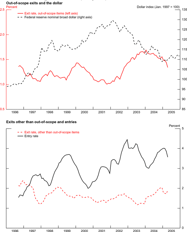
Figure 2: Coefficients on lags of the exchange rate in pass-through regressions in baseline Calvo and menu-cost models
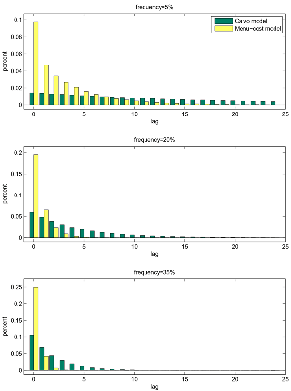
Figure 3: Cumulative contribution of coefficients on lagged exchange rate variables under selective exit (e=0.25)
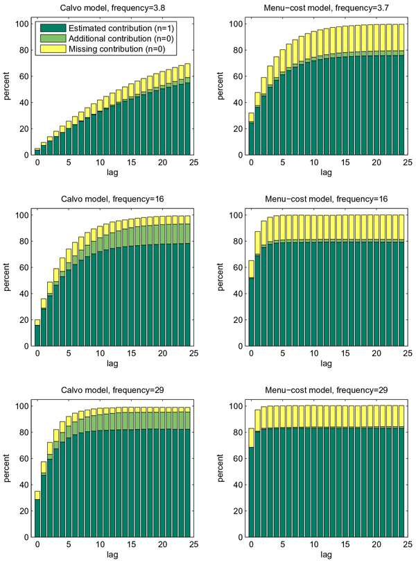
Figure 4: Cumulative contribution of coefficients on lagged exchange rate variables in Calvo model under severe product replacement bias (n=1, s=0.05)
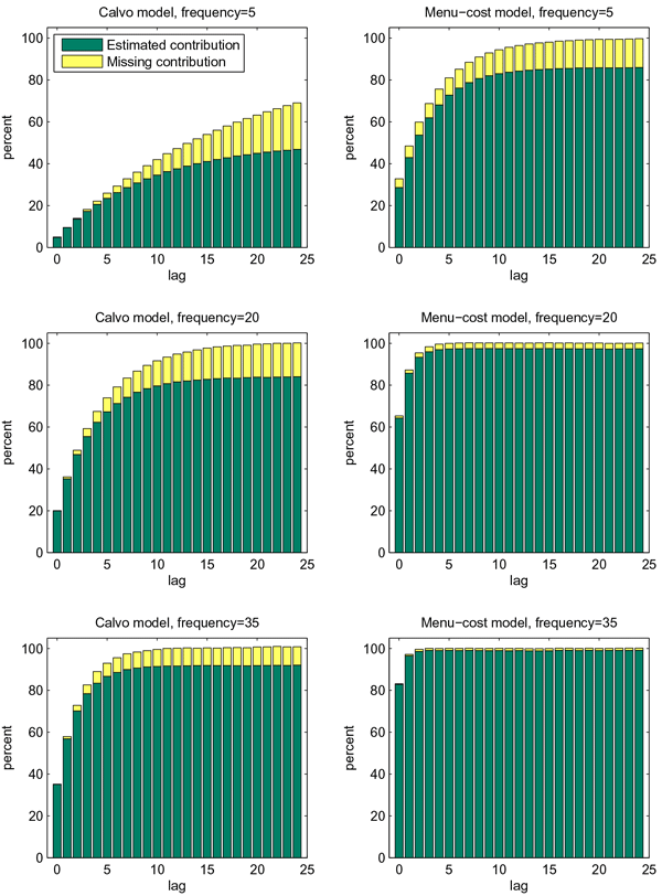
Figure 5: Pass-through to imported finished goods prices following a 1-percent depreciation of the dollar (by 3-digit Enduse categories)
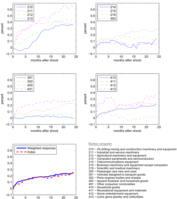
Figure 6: Pass-through to imported finished goods prices following a 1-percent depreciation of the dollar: models versus data
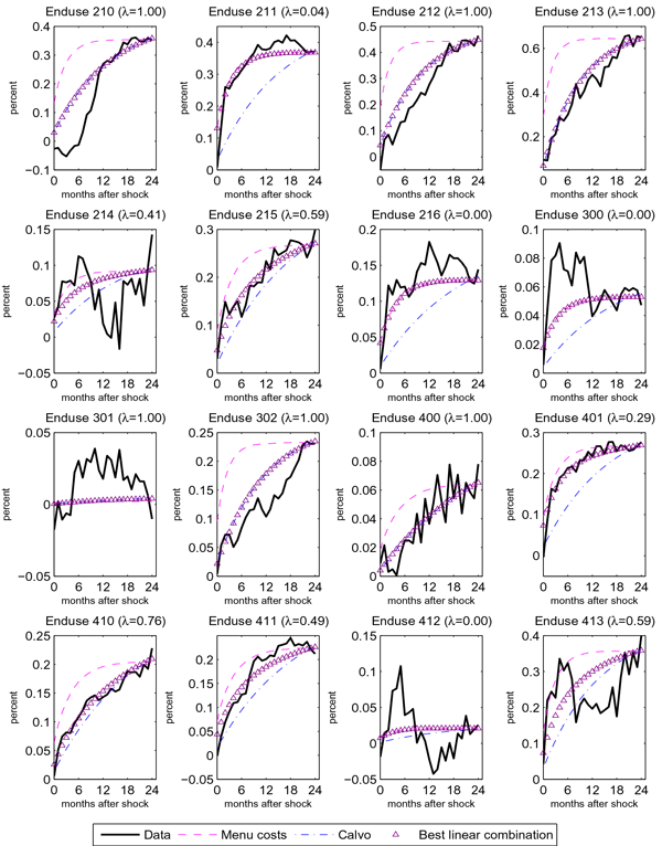
Notes: The figure shows the empirical impulse response for three-digit Enduse categories along with calibrated impulse responses in the Calvo and the menu-cost models. The figure also shows the combination of models minimizing over λ IRFCalvo + (1 - λ) IRFMC - IRFdata over ∈ [0, 1], where is the Euclidian distance and IRFCalvo, IRFMC, and IRFdata are the impulse responses in the Calvo model, the menu-cost model, and the data.
Figure 7: Upper bounds on exchange rate pass-through to imported finished goods
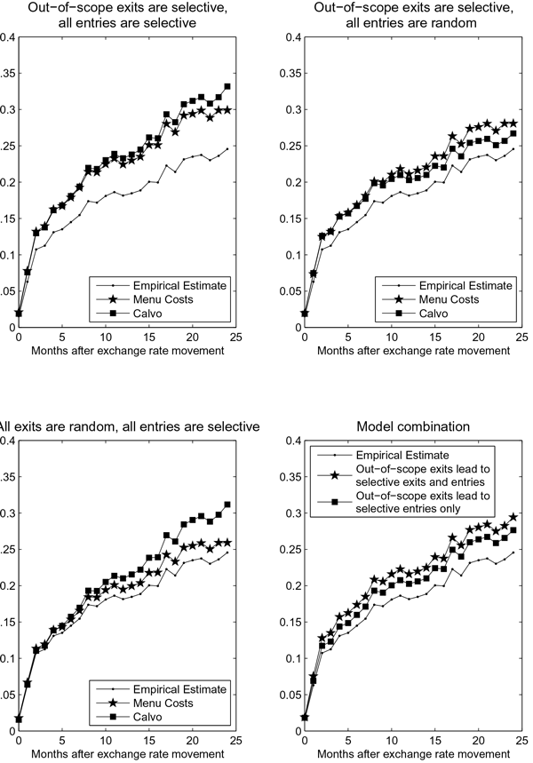
Figure 8: Impact of delaying entries on cumulative contribution of coefficients on lagged exchange rate variables under severe product replacement bias (n=1, s=0.05)
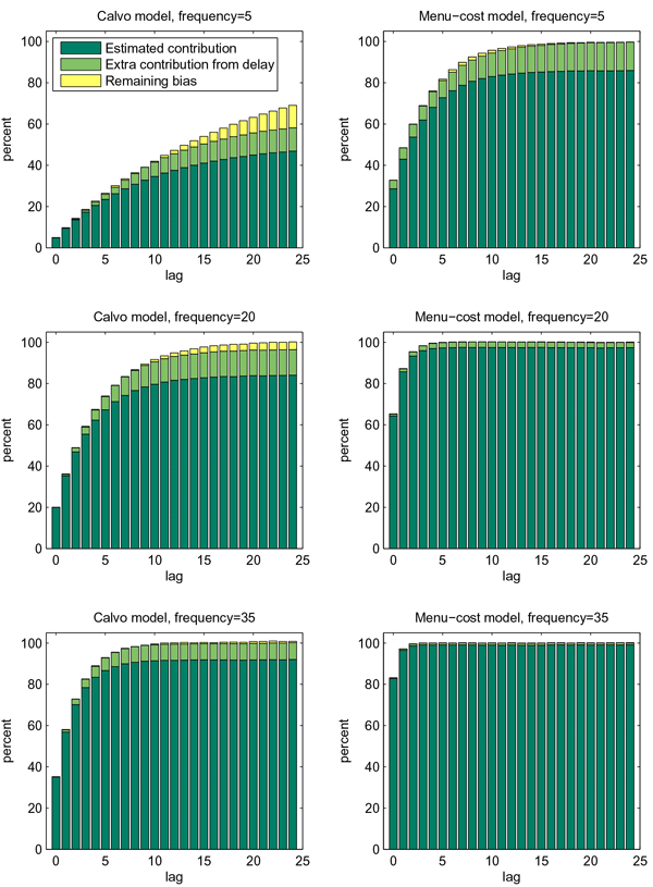
Figure 9: Impact of delaying entries on cumulative contribution of coefficients on lagged exchange rate variables under selective exits and random entries (n=0, e=0.25)
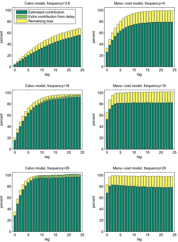
Figure 10: Alternative price indexes and pass-through
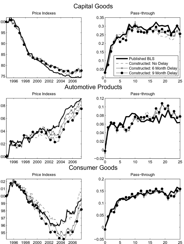
Figure 11: Marginal probabilities of observations usable to computed inflation in period in the Calvo model with iid exchange rate innovations
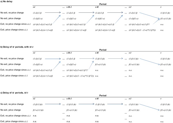
Notes: This figure shows the marginal probabilities in periods
![]() to
to ![]() of items whose
price can be used to compute inflation in period
of items whose
price can be used to compute inflation in period ![]() .
The arrows illustrate the various paths through which a movement in
the exchange rate in period
.
The arrows illustrate the various paths through which a movement in
the exchange rate in period ![]() could be
reflected as a nonzero contribution to inflation in period
could be
reflected as a nonzero contribution to inflation in period
![]() . The upper, middle, and lower panels show
the case in which observations entering the sample are delayed by
0,
. The upper, middle, and lower panels show
the case in which observations entering the sample are delayed by
0, ![]() , and
, and ![]() period(s), respectively.
period(s), respectively.
Figure 12: Correction factors for the cumulative index response to an exchange rate shock in a Calvo model with real rigidities
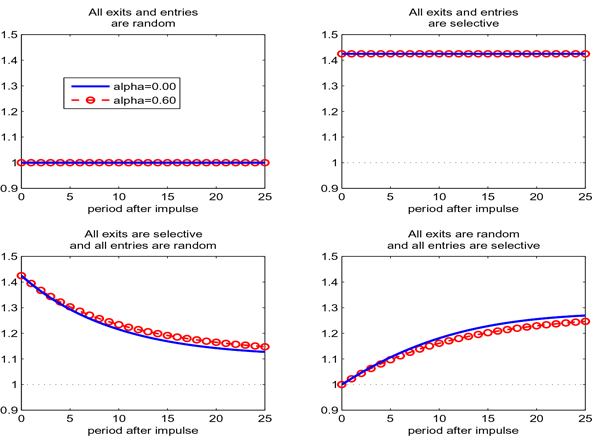
Notes: This figure shows the theoretical correction factors one would apply to the cumulative import price index response to a one-time jump in the exchange rate. The model assumes Calvo pricing with an exogenous frequency of price changes of 15 percent and a substitution rate of 5 percent. The real rigidity parameter is specified as in appendix B.
Footnotes
1. These papers include Atkeson and Burstein (2008), Gopinath, Itskhoki, and Rigobon (2010), Gopinath and Itskhoki (2010), and Gust, Leduc, and Vigfusson (2010). Return to text
2. We focus on the response of import prices over the first two years following an exchange rate movement, which corresponds to the policy horizon of most central banks and international institutions. Near-term horizons are arguably the most relevant when using impulse responses to differentiate among models. For example, the implications of producer and local currency pricing are most stark in the first few years after a shock. Return to text
3. For an introduction to the economics of new goods, see the volume edited by Breshnahan and Gordon (1996). Gordon (2006) and the conference summaries of the Ottawa Group provide overviews of subsequent research. Return to text
4. For a given item, reporting firms typically do not provide a transaction price every month. The BLS imputes an item's missing price by either carrying forward the last reported price or by adjusting it by the average price change for the same firm and product category. Return to text
5. For instance, if there are two items sampled at a firm, one of which has a 90 percent sales share and the other a 10 percent sales share, allocating weights uniformly would over-weight the smaller item. When constructing its aggregate price indexes, BLS corrects for this phenomenon with item-level probability weights. Return to text
6. In some instances, the firm can provide an alternative item that meets BLS sampling needs (called "replaced"), though that new item would still be recorded as a separate entry. Return to text
7. For instance, during biennial sample redrawings, some disaggregate product categories may be retired from further sampling but their items may remain in the index until their planned phaseout. Where outgoing and incoming product groups are dissimilar, the benefit to overlapping their items is unclear. Return to text
8. Incomplete reporting for item discontinuation reasons in the database made available to outside researchers by the IPP truncates our sample at its beginning and end. October 1995 is the first month for which the discontinuation reason field is populated, while the months following April 2005 contain incomplete information about exits. Return to text
9. Doing so assigns the average item frequencies for sampled items and products to those not sampled within the same industry. Return to text
10. An alternative weighting scheme would
be to use the BLS product weights, which are akin to annual import
values at the Harmonized System 10-digit (HS10) level, spread
evenly across items within each product. The end-use weights for a
given month would be the sum total of the individual item weights
across items and HS10 products within that end-use. However, due to
incomplete weight data for petroleum (Enduse 100), that method
tends to under-weight those high-frequency products in the
aggregate statistics. Otherwise, at the end-use level, the measures
are quite similar.
Also, ignoring the BLS probability weights for items and firms
within each HS10 product, as we do, does not drastically change the
summary statistics. Probability-weighted and unweighted statistics
are available upon request. Return to
text
11. The exit rates shown in the figure are 12-month moving averages. Return to text
12. Some micro price studies include carried forward prices in their count of price observations (i.e., the denominator of the frequency formula), while others do not. We choose to use such price observations. One benefit of this approach is that the number of usable observations from one month to the next is directly determined by the number of entries and exits. If we instead excluded imputed prices, then our statistics would need to account for the fact that some quotes are inactive. Our decision makes price changes, exits, and entries somewhat less frequent than if imputations were excluded. The broad findings of the paper do not hinge on this methodological choice, however. Return to text
13. Our price-setting rule abstracts from forward-looking concerns, which greatly simplifies the exposition. Monthly exchange rate innovations are only weakly correlated, so our purely backward-looking rule should nevertheless capture central features of micro price adjustments in response to exchange rate movements. Return to text
14. In practice, the frequency of price changes and the degree of exchange rate pass-through appear interrelated. Gopinath and Itskhoki (2010) present evidence that items with relatively low frequencies of price changes tend to be associated with relatively low rates of pass-through. Return to text
15. In principle, mismeasured changes in quality can result in either upward or downward biases, depending on whether the quality change is underestimated (e.g., ignoring improvements in a computer's processing power) or overestimated (e.g., failing to account for the use of lower-quality components). In practice, the quality change bias is associated with a systematic overestimation of inflation (see BLS (1997b) and Bils (2010), among many others). By contrast, in our canonical case with all exits and entries being selective, only a fraction of the aggregate price adjustment is recorded, so that inflation is underestimated when it is positive, and overestimated when it is negative. As a result, the price response to a shock is underestimated, which would not be the case if inflation was mismeasured by a fixed amount every period. Return to text
16. Greenlees and McClelland (2011) offer evidence that exiting food items in the CPI have larger price changes (including zeros) on average than continuing items. They also argue that current CPI techniques may overestimate the extent of quality adjustments for these categories. Return to text
17. When all exits are selective and all
entries are random, the long-run response of the index is given by
![]() . The
same conclusion applies for the general case, for which the
long-run response is
. The
same conclusion applies for the general case, for which the
long-run response is
 . This response is smaller than
 ![]() and increasing
in the fraction of entering items randomly sampled from the
universe. Randomizing entries thus reduces the downward bias
without eliminating it entirely. Return
to text
and increasing
in the fraction of entering items randomly sampled from the
universe. Randomizing entries thus reduces the downward bias
without eliminating it entirely. Return
to text
18. We thank Emi Nakamura and Jon Steinsson for pointing out this link in an email correspondence. Return to text
19. Our simple specification does not allow for variation in the magnitude of the response over time, a restriction imposed in part due to the short period over which monthly import price data are available. Taking advantage of the longer time coverage of quarterly series, several authors have documented a decline in pass-through rates in recent decades (e.g., Marazzi et al., 2005), including for finished goods (see Gust et al., 2010). As mentioned earlier, we find little evidence that an increase in the occurrence of selective exits and entries could account for that pattern. Return to text
20. We assume that individual (nonzero) price changes leading to exits have the same distribution as those for items remaining in the sample. Whether this is the case in practice remains an open question. Return to text
21. That said, equation (8) is likely misspecified for material-intensive goods because movements in commodity prices can affect both the exchange rate and material-intensive goods prices. Return to text
22. Allowing the substitution rate to vary across 3-digit Enduse categories based on the entry rates displayed in table 1 has only a minor impact on our findings. Return to text
23. We exclude from our comparisons the possibility that exits are selective and entries are random because Nakamura and Steinsson (2011) do not model the exit decision explicitly. Return to text
24. In particular, when
![]() , our
equation 20 is an
implementation of equation 20 in Nakamura and Steinsson (2011)
under our distributional assumptions for the frequency of price
changes. Return to text
, our
equation 20 is an
implementation of equation 20 in Nakamura and Steinsson (2011)
under our distributional assumptions for the frequency of price
changes. Return to text
25. We also note that using only 6 lags of quarterly exchange rate movements in the regression would be insufficient to precisely estimate long-run pass-through if the data were truly generated from a Calvo model, even absent any product replacement bias. For import prices excluding oil, 0.79 percent of the true long-run response is realized after 6 quarters, a figure that shrinks to 0.68 when we focus on finished goods. A failure to use a sufficiently large number of lags in the regression would thus be a source of downward bias in the estimation of long-run pass-through. Return to text
This version is optimized for use by screen readers. Descriptions for all mathematical expressions are provided in LaTex format. A printable pdf version is available. Return to text