Skip to: [Printable Version (PDF)]

Board of Governors of the Federal Reserve System
International Finance Discussion Papers
Number 1062r, June 2013 --- Screen Reader Version*

A State-Dependent Model for Inflation Forecasting¹

Andrea Stella and James H. Stock

NOTE: International Finance Discussion Papers are preliminary materials circulated to stimulate discussion and critical comment. References in publications to International Finance Discussion Papers (other than an acknowledgment that the writer has had access to unpublished material) should be cleared with the author or authors. Recent IFDPs are available on the Web at http://www.federalreserve.gov/pubs/ifdp/. This paper can be downloaded without charge from the Social Science Research Network electronic library at http://www.ssrn.com/.

Abstract:

We develop a parsimonious bivariate model of inflation and unemployment that allows for persistent variation in trend inflation and in the non-accelerating inflation rate of unemployment. The model, which consists of five unobserved components including the trends) with stochastic volatility, implies a time-varying vector autoregression model for changes in the rates of inflation and unemployment. The implied backwards-looking Phillips curve has a time-varying slope that is steeper in the 1970s than in the 1990s. Pseudo out-of-sample forecasting experiments indicate improvements upon univariate benchmarks. Since 2008, the implied Phillips curve has become steeper and the the non-accelerating inflation rate of unemployment has increased.

Keywords: Inflation forecasting, Phillips curve, trend-cycle model, NAIRU

JEL classification: C53, E37

1  Introduction

Recent research on inflation forecasting in the postwar United States suggests empirical support for four conclusions. First, it is difficult to improve over univariate time series models, at least on average. This point was made most dramatically by Atkeson and Ohanian (2001), who showed that a random walk model for the annual rate of inflation beat multivariate models using measures of economic activity as predictors (Phillips curve models). Second, when multivariate models do improve upon univariate models, they tend to do so episodically. For example, Stock and Watson (2009, 2010) and Dotsey, Fujita, and Stark (2011) find that Phillips curve models improve upon univariate models during periods of slack, but typically not otherwise. Ball and Mazumder (2011) suggest that the time variation in the Phillips Curve slope occurs at a decadal, not business cycle, frequency, although they only consider contemporaneous relations, not forecasting specifications. Third, it is not clear whether the apparent episodic predictability is better modeled as a stationary nonlinear model, as suggested by Barnes and Olivei (2003), Fuhrer and Olivei (2010), and Stock and Watson (2010), or as a result of time variation (or, relatedly, state dependence with time-varying unobserved states) as in Cogley and Sargent (2002, 2005), Cogley, Primiceri, and Sargent (2010), D'Agostino, Gambetti and Giannone (2010), Levin and Piger (2004), Stock and Watson (2007), and Ball and Mazumder (2011), or both as in Granger and Jeon (2011). Fourth, predictors other than activity measures appear to be generally unreliable and unpromising (for a survey, see Stock and Watson (2009)). One reason for this murky state of affairs is that there is limited variation in the data with which to identify the nature of the time variation and/or nonlinearity, and that models with many parameters tend to be overwhelmed by estimation uncertainty and thus produce poor forecasts.

This paper takes up the challenge of developing a tightly parameterized model that is capable of capturing the time-variation in the inflation-activity predictive relation. The specific model proposed here builds on two streams of literature. The first stream is papers that model the trend component of inflation, which can be thought of as target inflation, as a latent random walk; recent examples of papers that take this approach include Stock and Watson (2007), Cogley and Sbordone (2008), Sbordone, Tambalotti, Rao, and Walsh (2010), Cogley, Primiceri, and Sargent (2010), and D'Agostino, Gambetti and Giannone (2010). Specifically, we follow Stock and Watson (2007) by adopting a stochastic volatility model that allows the variance of trend inflation to change over time, in effect allowing the degree of anchoring of inflation expectations to vary over time. The second literature stream is work on estimating the natural rate of unemployment, in which the natural rate (typically interpreted as the non-accelerating inflation rate of unemployment, the NAIRU) is modeled as a latent random-walk trend in the rate of unemployment. This latent time-varying NAIRU is modeled as a random walk in Staiger, Stock, and Watson (1997) and Gordon (1998), and we adopt that specification here with the extension that the innovation variance to the NAIRU also can evolve over time as a stochastic volatility process. The only paper we are aware of that merges both a time-varying trend in inflation and a time-varying NAIRU is Harvey (2011). Relative to Harvey (2011), we extend the model to include time-varying volatility, so that the projection coefficients (the Phillips Curve in terms of the observables) vary over time in a parsimonious specification.

In the model of this paper, the deviations of the inflation and unemployment rates from their trends - that is, the inflation and unemployment gaps - are linked through a common cyclical component, and the inflation and unemployment rates are both potentially measured with error. The variances of the disturbances to the latent components are modeled as stochastic volatility processes. Given the innovation variances of the latent components, the model implies a vector autoregressive (VAR) representation of the changes of the rates of inflation and unemployment, the inflation equation of which is a forecasting Phillips curve. Because the innovation variances evolve over time, the implied VAR parameters also evolve, which implies a backwards-looking Phillips curve forecasting relation with time-varying coefficients. Our base model has three parameters to be estimated, plus three tuning parameters which are weakly identified and are therefore fixed.

Other than Harvey (2011), the models most closely related to ours are those in Cogley, Primiceri, and Sargent (2010), D'Agostino, Gambetti and Giannone (2010) and in Granger and Jeon (2011). Cogley, Primiceri, and Sargent (2010) specify a trivariate VAR of the rates of inflation, unemployment, and interest, with 21 time-varying VAR coefficients and 24 stochastic volatility processes; D'Agostino, Gambetti and Giannone (2010) use the same model, but with only 3 stochastic volatility processes. With an eye towards forecasting, we focus on a much tighter parameterization, with two time-varying parameters (the trends), and, in our base model, three stochastic volatility processes. Granger and Jeon (2011) consider time-varying parameter models without stochastic volatility for the inflation equation (the Phillips curve), but (like Cogley, Primiceri, and Sargent (2010)), their specifications fix the lag length at 2 whereas the VAR representation implied by our model is infinite-order with time-varying coefficients at all lags, thereby allowing for time-varying dependence.

Because our model nests and extends existing work, some of our results connect with the existing literature. Consistent with Stock and Watson (2007, 2010), we find considerable time variation in the innovation to the permanent component of inflation, consistent with drifting expectations in the 1970s and anchored expectations in the 2000s. Consistent with Staiger, Stock, and Watson (1997) and Gordon (1998), we find low frequency variation in the NAIRU, with the NAIRU highest in the 1970s and early 1980s, and lowest in the 1990s. The novel aspects of our results are the implied time-varying projections and simulated forecasting performance. The base model estimates considerable time variation in the slope of the predictive Phillips curve, which is measured as the sum of the coefficients on unemployment in the linear projection of inflation on current and past changes of unemployment, after subtracting estimated target inflation and the NAIRU. The empirical time variation is at a lower frequency than the cyclical variation suggested in Stock and Watson (2009, 2010) and Dotsey, Fujita, and Stark (2011), and the pattern is also different than the decadal swings of Ball and Mazumder (2011): according to the estimates in Section 4, the Phillips Curve slope is moderate in the 1960s, steeper in the 1970s and early 1980s, flat for the Great Moderation period. In the most recent data, the predictive Phillips Curve is estimated to be as steep in 2010 as it was in the 1970s and the NAIRU is rising.

We also report the results of a pseudo out-of-sample forecasting comparison of the performance of this model, relative to the Atkeson-Ohanian (2001) random walk forecast and the Stock-Watson (2007) univariate unobserved components-stochastic volatility model. The base model generally outperforms these two univariate benchmarks, particularly at short forecasting horizons. This finding is robust to various modifications of the base model. The model is estimated using a Bayesian Gibbs sampling procedure; since the posterior distribution of the model is rather complex and hard to sample from, we draw the parameters and latent variables sequentially from tractable conditional posterior distributions.

The rest of this paper is organized as follows. The model and identification are discussed in Section 2. Section 3 discusses estimation by Bayesian Markov Chain Monte Carlo methods, and Section 4 presents the results. Section 5 concludes.

2  The Model

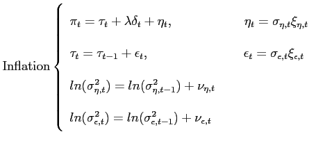
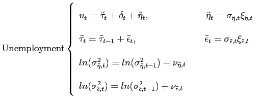
We model unemployment and inflation symmetrically as the sum of a random walk trend, a common cyclical component and serially uncorrelated measurement error, so that the two observed series are represented in terms of five unobserved components. In the most general model the variances of the innovations of the unobserved components all follow stochastic volatility processes, with latent variance processes that evolve over time. This multivariate unobserved components Ð stochastic volatility (UC-SV) model is:

$$\textrm{Inflation}\left\{ \begin{array}{l} \pi_{t} = \tau_{t} + \lambda \delta_{t} + \eta_{t}, \>\>\>\>\>\>\>\>\>\>\>\>\>\>\>\>\>\>\>\>\>\>\>\> \eta_{t} = \sigma_{\eta, t } \xi_{ \eta, t } \ \tau_{t} = \tau_{t-1} + \epsilon_{t}, \>\>\>\>\>\>\>\>\>\>\>\>\>\>\>\>\>\>\>\>\>\>\>\>\>\>\>\>\>\>\>\> \epsilon_{t} = \sigma_{\epsilon, t } \xi_{ \epsilon, t } \ ln(\sigma_{\eta, t}^{2}) = ln(\sigma_{\eta, t-1}^{2}) + \nu_{\eta, t} \ ln(\sigma_{\epsilon, t}^{2}) = ln(\sigma_{\epsilon, t-1}^{2}) + \nu_{\epsilon, t} \end{array} \right.$$ (1)

$$\textrm{Unemployment}\left\{ \begin{array}{l} u_{t} = \tilde{\tau}_{t} + \delta_{t} + \tilde{\eta}_{t}, \>\>\>\>\>\>\>\>\>\>\>\>\>\>\>\>\>\>\>\>\>\>\>\>\>\> \tilde{\eta}_{t} = \sigma_{\tilde{\eta}, t} \xi_{\tilde{\eta}, t } \ \tilde{\tau}_{t} = \tilde{\tau}_{t-1} + \tilde{\epsilon}_{t}, \>\>\>\>\>\>\>\>\>\>\>\>\>\>\>\>\>\>\>\>\>\>\>\>\>\>\>\>\>\>\> \tilde{\epsilon}_{t} = \sigma_{\tilde{\epsilon}, t} \xi_{\tilde{\epsilon}, t } \ ln(\sigma_{\tilde{\eta}, t}^{2}) = ln(\sigma_{\tilde{\eta}, t-1}^{2}) + \nu_{\tilde{\eta}, t} \ ln(\sigma_{\tilde{\epsilon}, t}^{2}) = ln(\sigma_{\tilde{\epsilon}, t-1}^{2}) + \nu_{\tilde{\epsilon}, t} \end{array} \right.$$ (2)

$$\textrm{Common cyclical component}\left\{ \begin{array}{l} \delta_{t} = \alpha_{1} \delta_{t-1} + \alpha_{2} \delta_{t-2} + \zeta_{t}, \>\>\>\>\>\>\>\> \zeta_{t} = \sigma_{\zeta, t } \xi_{ \zeta, t } \ ln(\sigma_{\zeta, t}^{2}) = ln(\sigma_{\zeta, t-1}^{2}) + \nu_{\zeta, t} \end{array} \right.$$ (3)

where $\xi_{t} = \{ \xi_{ \eta, t } , \xi_{ \epsilon, t }, \xi_{ \tilde{\eta}, t }, \xi_{ \tilde{\epsilon}, t }, \xi_{ \zeta, t }\}$ is i.i.d. N(0,I) and $\nu_{t} = \{ \nu_{ \eta, t }, \nu_{ \epsilon, t }, \nu_{ \tilde{\eta}, t }, \nu_{ \tilde{\epsilon}, t }, \nu_{ \zeta, t } \}$ is i.i.d. $N(0,\gamma I)$ and $\xi_{t}$ and $\nu_{t}$ are independent.

With $\lambda = 0$, the inflation block of the model is the same as in Stock and Watson (2007); with $\lambda \neq 0$, the inflation block can be interpreted as a Phillips curve. The unemployment block parallels the inflation block.

The multivariate UC-SV model can be interpreted in various ways. The trend in inflation $\tau_{t}$ can be thought of as representing inflation expectations (which makes (1) akin to a New Keynesian Phillips Curve (NKPC); this is the interpretation given in Stock and Watson (2007, 2010)) or as a Central Bank's inflation target (e.g. as in Cogley and Sbordone (2008) and Sbordone, Tambalotti, Rao, and Walsh (2010)). The trend in the unemployment rate, $\tilde{\tau}_{t}$, provides a time-varying NAIRU, in the sense that $\delta_{t}$ is the unemployment gap that potentially affects inflation. The random walk specification for the NAIRU is the same specification as in Staiger, Stock and Watson (1997) and Gordon (1998), extended to allow for stochastic volatility. The assumption that the innovations to inflation expectations and to the NAIRU are independent reflects the distinct institutional and economic processes that underpin a Central Bank's long-term inflation target and credibility on the one hand, and, on the other hand, the changes in productivity and labor market composition that are generally considered to drive the NAIRU. The independence of the serially uncorrelated disturbances $\epsilon_{t}$ and $\tilde{\epsilon}_{t}$ is motivated by viewing these as measurement error arising from the independent surveys from which the series are constructed. The common cyclical component $\delta_{t}$ links the inflation and unemployment gaps over business cycle frequencies, and $\lambda$ plays the same role in this model as does the coefficient on the activity variable in the NKPC, when the NKPC is specified in terms of an activity gap or the unemployment rate.

From a statistical perspective, the model provides a parsimonious parameterization of time variation in the joint process for inflation and unemployment, with four parameters ($\lambda$, $\alpha_{1}$, $\alpha_{2}$, $\gamma$). Given fixed values of the innovation variances, that is, at a given point in time, the unobserved components model implies specific joint autocovariances of ( $\Delta \pi_{t}$, $\Delta u_{t}$), which in turn implies a vector autoregression (VAR) representation of ( $\Delta \pi_{t}$, $\Delta u_{t}$). The parameters of the VAR representation depend on the innovation variances because the VAR coefficients essentially arise from a multivariate signal extraction problem, which in turn depends on the various signal-to-noise ratios.²

Assuming $\alpha_{1}$, $\alpha_{2}$, $\gamma$ are nonzero, the model is identified. The likelihood, however, turns out to be quite flat in some of the parameters. We therefore imposed the following three restrictions:

i  $\gamma$ = 0.2;

ii   $\sigma_{\tilde{\epsilon}}^{2}$ = 0.01; and

iii   $\sigma_{\tilde{\eta}}^{2}$ = 0.2.

Restriction (i) is taken from Stock and Watson (2007), extended here to the multivariate system. Restriction (ii) eliminates stochastic volatility in the NAIRU. This restriction is consistent with the previous work cited above on unobserved components models of the NAIRU in which there was no evidence of time-varying low frequency variances. Restriction (iii) is imposed to resolve an empirical problem of separately estimating the measurement error and the cyclical component of the unemployment rate. Section 4 reports sensitivity analysis for various alternative treatments of $\sigma_{\tilde{\eta}}^{2}$, including time-varying estimation. With these three restrictions imposed, the model has three estimated parameters, $\alpha_{1}$, $\alpha_{2}$, and $\lambda$.

3  Estimation Strategy

The model is estimated using a Gibbs sampling procedure. The parameters and latent variables are divided in three blocks. In the first block, we draw the latent variables $\tilde{\tau}$, $\delta$ and $\tau$ conditioning on the inflation and unemployment series, the parameters, $\alpha_{1}$, $\alpha_{2}$, and $\lambda$, and the stochastic volatilities. We first determine the joint posterior distribution of inflation, unemployment and the three latent variables conditional on the parameters and the stochastic volatilities; we then sample from the conditional distribution of the latent variables. Next, we condition on the latent variables and the stochastic volatilities and we sample from the posterior of the parameters. We assume normal conjugate priors for the parameters, with zero mean and variance equal to 100. Also, $\alpha_{1}$ and $\alpha_{2}$ are constrained to be in the triangle $-1 \leq \alpha_{2} \leq 1 - \vert\alpha_{1}\vert$ so that the cyclical process $\delta_{t}$ is stationary. Finally we draw the stochastic volatilities a la Kim et al. (1998), conditioning on the latent variables and the parameters.³

4  Data Description and Empirical Results

The data set is quarterly from 1960Q1 to 2011Q3. Inflation is measured by the GDP deflator and the unemployment rate is the quarterly average of the monthly total civilian unemployment rate. The data are plotted in Figure 6.1.

4.1  In-Sample Results on Historical Time Variation

Figures 6.2 and 6.3 plot the estimated time paths of the volatilities that are not fixed under the base model; these and the following estimated time paths are posterior means and 95% intervals from the nonlinear, non-Gaussian smoother and are conditional on the full data set. The variance of the permanent innovation to inflation has an estimated time path that is similar to the one in Stock and Watson (2007), with the variance of the permanent component large in the 1970s and early 1980s and smaller in the 1960s, 1990s and early 2000s; these latter periods correspond to periods of relatively well-anchored inflation expectations. The variance of the transitory innovation in inflation shows more variability than in Stock and Watson (2007). The variance of the cyclical component follows a recognizable time path: it was large before the mid-1980s, it diminished during the Great Moderation, and it increased substantially since 2007 to pre-Great Moderation levels. It must be noted that the confidence intervals around the stochastic volatilities are wide, which means that there is considerable uncertainty on the conclusions regarding the time-varying patterns of volatility.

Estimates of the trend and common cyclical components are plotted in Figure 6.4. As in Stock and Watson (2007) and Cogley, Primiceri, and Sargent (2010), trend inflation closely tracks the low-frequency swings in inflation. The estimated NAIRU (Figure 6.5a), fluctuates through a range of just over one percentage point. The NAIRU is estimated to be greatest during the 1970s, to be lowest during the early 2000s, and to be rising recently. Figure 6.5b shows the estimated NAIRU when we relax restriction (iii). Estimating $\sigma_{\tilde{\eta}}^{2}$ does not change the low frequency properties of the estimated NAIRU, but it adds considerable high frequency noise to it. When we allow $\sigma_{\tilde{\eta}}^{2}$ to be unrestricted, the estimation attributes all the high frequency noise in the unemployment rate to $\tilde{\tau}$, rather than to the measurement error $\tilde{\eta}$. We think that this result is due to weak identification and we therefore fix $\sigma_{\tilde{\eta}}^{2}$ to 0.2. The forecasting performance of the model is only marginally affected by this restriction, as shown later in the paper.

Figure 6.6 presents the posterior distributions of the parameters. Most notably, the posterior for $\lambda$ has essentially all its mass less than zero, with a posterior mean of -0.37 and a 95% Bayesian credible set of (-0.58, -0.17). The posteriors for all three parameters are much tighter than the priors, with different means.

One aim of this model is to allow for the possibility of time-varying VAR coefficients, in particular for a time-varying slope of the Phillips curve. Figure 6.7 plots the slope of the Phillips curve, as measured by the time-varying sum of the coefficients on lagged unemployment in the implied VAR for detrended inflation and unemployment, ( $\pi_{t} - \tau_{t}$, $u_{t} - \tilde{\tau}_{t}$ ). The Phillips curve slope $\kappa$ is steepest (the implied sum-of-coefficients is most negative) in the 1970s, is the flattest in the 1990s, and has increased in steepness since 2007. It must be noted that there is considerable uncertainty around the estimate of $\kappa$, as shown by the 95% confidence intervals.

4.2  Pseudo Out-of-Sample Forecast Evaluation

This section reports the results of a pseudo out-of-sample inflation forecasting exercise. Specifically, the model parameters were estimated using Gibbs sampling⁴, with a quarterly expanding estimation sample starting with 1960Q1 - 1979Q4. The analysis focuses on the base model of Section 2 and one variant described below. We also consider three univariate benchmark models, the Stock-Watson (2007) univariate UC-SV model and two versions of the Atkeson-Ohanian (2001) quarterly random walk model. The first AO model (AO(i)) forecasts $h$-quarter ahead inflation using lagged four-quarter inflation; the second AO model (AO(ii)) forecasts $h$-quarter ahead inflation using lagged $h$-quarter inflation. For horizons greater than one quarter, the object being forecast is the multi-period percentage rate of inflation at annual rates, for example at 4-quarters the object of interest is $100ln(P_{T+4}/P_{T})$. This pseudo out-of-sample exercise uses the most recent vintage of data with no real-time data adjustments.

The results are summarized in Table 1 through 4. The first row of each block reports the pseudo out-of-sample root mean squared forecast error (RMSFE) of the univariate UC-SV model, and the remaining rows report RMSFEs relative to the UC-SV benchmark. Results are reported for 1, 2, 4, and 8-quarter ahead forecasts, and for various subsamples.

Over the full sample, the base model provides modest improvements over the UC-SV and AO models, particularly at the one- and two-quarter horizons. Table 1 also reports results for three variants of the base model. The first variant provides a different treatment of $\sigma_{\tilde{\eta}}^{2}$ (see (iii) in Section 2), allowing $\sigma_{\tilde{\eta}}^{2}$ to be estimated. This change generally makes little difference to the pseudo out-of-sample forecast RMSFEs, a result that is consistent with the difficulty we found in identifying this parameter using the full data set; a notable exception is represented by the 2000s, when the model with unrestricted $\sigma_{\tilde{\eta}}^{2}$ does better. The second and third variants allow for a more flexible specification for how $\delta_{t}$ enters the inflation equation (1), in particular, the term $\lambda \delta_{t}$ in (1) is replaced by the distributed lag, $\lambda_{1} \delta_{t} + \lambda_{2} \delta_{t-1} + \lambda_{3} \delta_{t-2}$ ; $\sigma_{\tilde{\eta}}^{2}$ is fixed to 0.2 in the second variant and estimated in the third. The model with a distributed lag does slightly better, above all in the 1990s.

5  Conclusions

We consider these results to be encouraging. The multivariate UC-SV model captures several of the features found in the inflation forecasting literature, most notably a time-varying state-dependent Phillips curve. The time-varying latent variables have natural interpretations as inflation expectations (or target inflation), the NAIRU, and a common cyclical component. The pseudo out-of-sample forecasting exercise suggests that this tightly parameterized model can improve upon the forecasts of what we understand to be the best univariate models.

6  Figures and Tables

Figure 6.1a. U.S. GDP Deflator Inflation and Unemployment Rates, Quarterly, 1960Q1- 2011Q3: Rate of Inflation (%, Annual Rate)

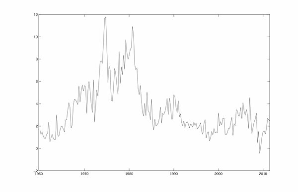
Figure 6.1b. U.S. GDP Deflator Inflation and Unemployment Rates, Quarterly, 1960Q1- 2011Q3: Rate of Unemployment (%, Annual Rate)

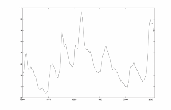
Figure 6.2a. Posterior Mean and 95% Interval of Time-Varying Variances of Innovations: Variance of Permanent Innovation to Inflation

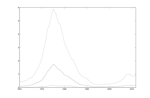
Figure 6.2b. Posterior Mean and 95% Interval of Time-Varying Variances of Innovations: Variance of Transitory Innovation to Inflation

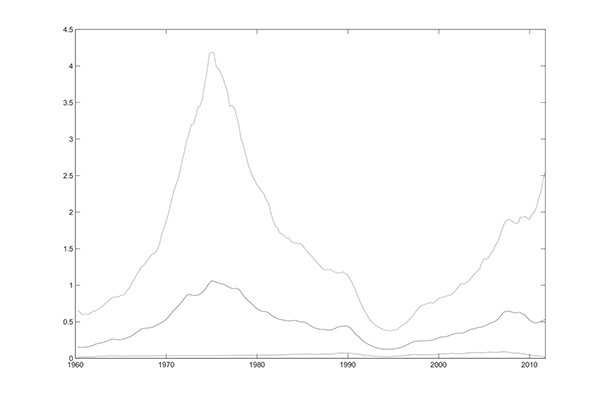
Figure 6.3. Posterior Mean and 95% Interval of Time-Varying Variances of Innovations: Variance of Innovation to Cyclical Component

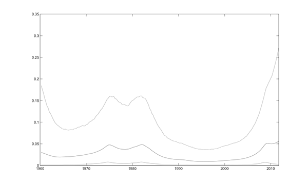
Figure 6.4a. Posterior Mean and 95% Interval of Unobserved Components: τ

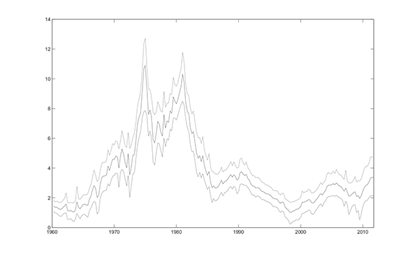
Figure 6.4b. Posterior Mean and 95% Interval of Unobserved Components: δ

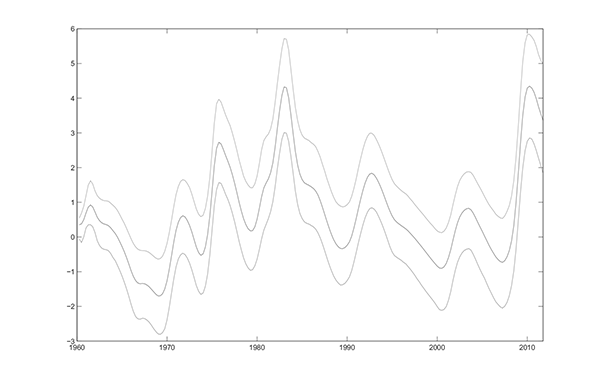
Figure 6.5a. Posterior Mean and 95% Interval of Unobserved Components: $\tilde{\tau}$

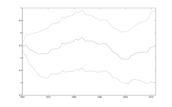
Figure 6.5b. Posterior Mean and 95% Interval of Unobserved Components: $\tilde{\tau}$ with $\sigma_{\tilde{\eta}}^{2}$ estimated

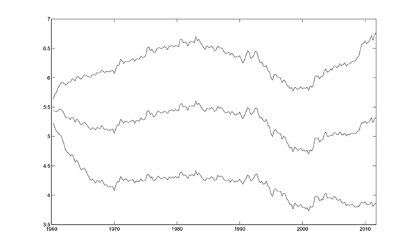
Figure 6.6a. Full-Sample Posterior and Diffuse Prior Distributions of Parameters :α₁

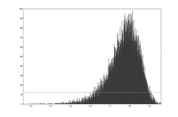
Figure 6.6b. Full-Sample Posterior and Diffuse Prior Distributions of Parameters: α₂

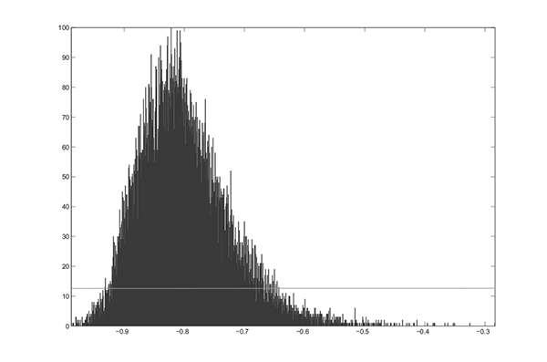
Figure 6.6c. Full-Sample Posterior and Diffuse Prior Distributions of Parameters: $\lambda$

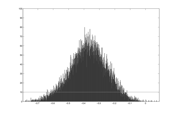
Figure 6.7. Slope of the Phillips curve κ for (π_t - τ) and 95% Interval

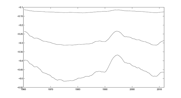
Table 1. Pseudo Out-of-Sample Forecasting Performance (1980:I-1989:IV)

Model	h=1	h=2	h=4	h=8
SW 2007	1.1375	1.1144	1.1813	1.5171
Relative RMSFE: SW 2007	1.0000	1.0000	1.0000	1.0000
Relative RMSFE: AO (i)	1.0652	1.0880	1.1172	1.0939
Relative RMSFE: AO (ii)	1.0292	0.9994	1.1172	1.2821
Relative RMSFE: No Lags - $\sigma_{\tilde{\eta}}^{2}$ = 0.2	0.9893	0.9904	0.9997	1.0330
Relative RMSFE: No Lags - $\sigma_{\tilde{\eta}}^{2}$ estimated	0.9894	0.9939	1.0079	1.0600
Relative RMSFE: 2 Lags - $\sigma_{\tilde{\eta}}^{2}$= 0.2	0.9902	0.9861	0.9885	1.0502
Relative RMSFE: 2 Lags - $\sigma_{\tilde{\eta}}^{2}$ estimated	0.9897	1.0004	1.0141	1.0737

NOTES: Entries are RMSFEs, relative to the Stock and Watson (2007) univariate UC-SV. Bold entries are the smallest relative RMSFE for the indicated series/period/horizon.

Table 2. Pseudo Out-of-Sample Forecasting Performance (1990:I-1999:IV)

Model	h=1	h=2	h=4	h=8
SW 2007	0.5818	0.5019	0.5083	0.6252
Relative RMSFE: SW 2007	1.0000	1.0000	1.0000	1.0000
Relative RMSFE: AO (i)	0.9948	0.9972	1.0470	1.0278
Relative RMSFE: AO (ii)	1.0988	1.0401	1.0470	1.1325
Relative RMSFE: No Lags - $\sigma_{\tilde{\eta}}^{2}$ = 0.2	0.9555	0.9186	0.9027	0.9603
Relative RMSFE: No Lags - $\sigma_{\tilde{\eta}}^{2}$ estimated	0.9547	0.9205	0.9022	0.9701
Relative RMSFE: 2 Lags - $\sigma_{\tilde{\eta}}^{2}$= 0.2	0.9652	0.9048	0.8491	0.9160
Relative RMSFE: 2 Lags - $\sigma_{\tilde{\eta}}^{2}$ estimated	0.9543	0.9149	0.8864	0.9633

NOTES: see the notes in Table 1

Table 3. Pseudo Out-of-Sample Forecasting Performance (2000:I-2011:III)

Model	h=1	h=2	h=4	h=8
SW 2007	0.8884	0.7906	0.7637	0.8175
Relative RMSFE: SW 2007	1.0000	1.0000	1.0000	1.0000
Relative RMSFE: AO (i)	1.0104	1.0114	1.0133	1.0021
Relative RMSFE: AO (ii)	1.1190	1.0230	1.0133	1.0760
Relative RMSFE: No Lags - $\sigma_{\tilde{\eta}}^{2}$ = 0.2	1.0021	1.0060	1.0068	0.9832
Relative RMSFE: No Lags - $\sigma_{\tilde{\eta}}^{2}$ estimated	0.9691	0.9501	0.9384	0.9420
Relative RMSFE: 2 Lags - $\sigma_{\tilde{\eta}}^{2}$= 0.2	1.0402	1.0733	1.1109	1.0720
Relative RMSFE: 2 Lags - $\sigma_{\tilde{\eta}}^{2}$ estimated	0.9508	0.9260	0.9207	0.9448

NOTES: see the notes in Table 1

Table 4. Pseudo Out-of-Sample Forecasting Performance (Whole Sample)

Model	h=1	h=2	h=4	h=8
SW 2007	0.8980	0.8384	0.8612	1.0602
Relative RMSFE: SW 2007	1.0000	1.0000	1.0000	1.0000
Relative RMSFE: AO (i)	1.0367	1.0539	1.0817	1.0689
Relative RMSFE: AO (ii)	1.0714	1.0117	1.0817	1.2276
Relative RMSFE: No Lags - $\sigma_{\tilde{\eta}}^{2}$ = 0.2	0.9895	0.9875	0.9911	1.0151
Relative RMSFE: No Lags - $\sigma_{\tilde{\eta}}^{2}$ estimated	0.9776	0.9719	0.9777	1.0277
Relative RMSFE: 2 Lags - $\sigma_{\tilde{\eta}}^{2}$= 0.2	1.0051	1.0061	1.0093	1.0398
Relative RMSFE: 2 Lags - $\sigma_{\tilde{\eta}}^{2}$ estimated	0.9713	0.9675	0.9754	1.0373

NOTES: see the notes in Table 1

References

Atkeson, A., & Ohanian, L. E. 2001, "Are Phillips Curves Useful for Forecasting Inflation?", Federal Reserve Bank of Minneapolis Quarterly Review, 25(1), 2-11.

Ball, L. & Mazumder, S. 2011, "Inflation Dynamics and the Great Recession", Brookings Papers on Economic Activity, 42(1), 337-405.

Bos, C. & Shephard, N. 2006. "Inference for Adaptive Time Series Models: Stochastic Volatility and Conditionally Gaussian State Space Form", Econometric Reviews, 25(2-3), 219-244.

Barnes, M. L. & Olivei, G. P. 2003, "Inside and Outside the Bounds: Threshold Estimates of the Phillips Curve", FRB of Boston New England Economic Review, 3-18.

Cogley, T., & Sargent, T. J. 2002, "Evolving Post-World War II U.S. Inflation Dynamics", In NBER Macroeconomics Annual 2001, ed. Ben S. Bernanke and Kenneth Rogoff, 331-388. Cambridge, MA: The MIT Press.

Cogley, T., & Sargent, T. J. 2005, "Drifts and Volatilities: Monetary Policies and Outcomes in the Post World War II U.S", Review of Economic Dynamics, 8(2), 262-302.

Cogley, T., & Sbordone, A. M. 2008, "Trend Inflation, Indexation, and Inflation Persistence in the New Keynesian Phillips Curve", American Economic Review, 98(5), 2101-26.

Cogley, T., Primiceri, G., & Sargent, T. J. 2010, "Inflation-Gap Persistence in the U.S.", American Economic Journal: Macroeconomics, 2, 43-69.

D'Agostino, A., Gambetti, L., & Giannone, D. 2011, "Macroeconomic Forecasting and Structural Change", Journal of Applied Econometrics, forthcoming.

Dotsey, M., Fujita, S., & Stark, T. 2010, "Do Phillips Curves Conditionally Help to Forecast Inflation?", manuscript, Federal Reserve Bank of Philadelphia.

Fuhrer, J.C. & Olivei, G. 2010, "The Role of Expectations and Output in the Inflation Process: An Empirical Assessment", FRB Boston Public Policy Brief Series, 10-2.

Geweke, J. 1991, "Efficient Simulation from the Multivariate Normal and Student-t Distributions Subject to Linear Constraints and the Evaluation of Constraint Probabilities", unpublished manuscript.

Ghysels, E., Harvey, A. & Renault, E., 1996. "Stochastic Volatility", Cahiers de recherche 9613, Universite de Montreal, Departement de sciences economiques.

Gordon, R. J. 1998, "Foundations of the Goldilocks Economy: Supply Shocks and the Time-Varying NAIRU", Brookings Papers on Economic Activity, 2, 297-333.

Granger, C.W.J. & Jeon, Y. 2011, "The Evolution of the Phillips Curve: A Modern Time Series Viewpoint", Economica, 78, 51-66.

Harvey, A.C. 1993, "Time Series Models", The MIT Press

Harvey, A.C. 2011, "Modelling the Phillips curve with unobserved components", Applied Financial Economics, 21(1-2), 7-17

Kim, S. and Harvey, A. 2003, "Computing Observation Weights for Signal Extraction and Filtering", Journal of Economic Dynamics and Control, 27, 1317-1333.

Kim, S., Shephard, N. & Chib, S. 1998, "Stochastic Volatility: Likelihood Inference and Comparison with ARCH Models", Review of Economic Studies, 65(3), 361-393.

Koopman, S.J., Shephard, N. and Chib, S. 1998, "Stochastic Volatility: Likelihood Inference and Comparison with ARCH Models", The Review of Economic Studies, 65(3), 361-93.

Koop, G. 2003, "Bayesian Econometrics", Wiley.

Levin, A. T., & Piger, J. M. 2004, "Is Inflation Persistence Intrinsic in Industrial Economics?", Working Paper Series 334. Frankfurt: European Central Bank.

Rossi, P. E., Allenby, G.M. & McCulloch, R. 2006, "Bayesian Statistics and Marketing", Wiley.

Sbordone, A., Tambalotti, A. & Walsh, K. R. 2010, "Policy Analysis Using DSGE Models: An Introduction", FRB of New York Policy Review, 23-43.

Shephard, N. 2005. "Stochastic Volatility", Economics Papers 2005-W17, Economics Group, Nuffield College, University of Oxford.

Staiger, D., Stock, J.H. & Watson, M.W. 1997, "How Precise are Estimates of the Natural Rate of Unemployment?" in C. Romer and D. Romer (eds.), Reducing Inflation: Motivation and Strategy, University of Chicago Press for the NBER, 195-242.

Stock, J. H. & Watson, M. 2007, "Why Has U.S. Inflation Become Harder to Forecast?", Journal of Money, Credit and Banking, 39(1), 3-33.

Stock, J. H. & Watson M. 2009, "Phillips Curve Inflation Forecasts", Ch. 3 in Understanding Inflation and the Implications for Monetary Policy, Jeffrey Fuhrer, Yolanda Kodrzycki, Jane Little, and Giovanni Olivei (eds). Cambridge: MIT Press.

Stock, J.H. & Watson, M.W. 2010, "Modeling Inflation after the Crisis", in Macroeconomic Policy: Post-Crisis and Risks Ahead, Proceedings of the Federal Reserve Bank of Kansas City 2010 Jackson Hole Symposium.

Footnotes

1.  The views in this paper are solely the responsibility of the authors and should not be interpreted as reflecting the views of the Board of Governors of the Federal Reserve System or of any other person associated with the Federal Reserve System. We would like to thank Eduardo Morales, Giulio Tiozzo, and Mark Watson for helpful comments. Return to text

2.  See Koopman and Harvey (2003) for a discussion of the relevant issues. Return to text

3.  Harvey and Renault (1995) and Shephard (2005) provide an excellent literature review of the econometrics of stochastic volatilities. Bos and Shephard (2006) discuss some of the issues involved in estimating unobserved component models with stochastic volatilities. Return to text

4.  The model was simulated 25,000 times after a burn-in period of 5,000 draws. Return to text

This version is optimized for use by screen readers. Descriptions for all mathematical expressions are provided in LaTex format. A printable pdf version is available. Return to text

Home | Economic research and data | Publications and education resources
Accessibility | Contact us
Last update: August 2, 2013