
Board of Governors of the Federal Reserve System
International Finance Discussion Papers
Number 1095, December 2013† --- Screen Reader Version*
Trade Reforms, Foreign Competition, and Labor Market Adjustments in the U.S.
NOTE: International Finance Discussion Papers are preliminary materials circulated to stimulate discussion and critical comment. References in publications to International Finance Discussion Papers (other than an acknowledgment that the writer has had access to unpublished material) should be cleared with the author or authors. Recent IFDPs are available on the Web at http://www.federalreserve.gov/pubs/ifdp/. This paper can be downloaded without charge from the Social Science Research Network electronic library at http://www.ssrn.com/.
Abstract:
Using data on trade-induced displacements, this paper documents that locations facing more foreign competition in the U.S. have: higher job destruction rates, lower job creation rates, and thereby lower employment rates. In contrast to standard trade theory, a model with variable markups and heterogeneous segmented labor markets is consistent with these facts. Foreign competition has a correlated effect on job destruction and job creation precisely because the most vulnerable locations also have lower productivity. Following an unexpected trade liberalization with limited mobility, employment sharply falls in the worse hit locations while welfare and employment increase in the aggregate.
Keywords: Foreign competition, nonemployment, job flows, spatial heterogeneity
JEL classification: F16, F66, G64
1 Introduction
In international trade, the reallocation of production factors like labor is essential for the gains from trade. The effects of trade reforms therefore depend crucially on how labor is reallocated within and across labor markets. Even though labor markets are certainly geographic in nature, geographically segmented labor markets with unemployment have not been modeled in standard trade theory. Recent evidence, however, suggests that the labor market effects of trade are uneven across locations. In particular, Autor et al. (2013b) find that U.S. localities with higher import penetration also experience lower employment. In the aggregate, Dutt et al. (2009) show that trade openness is associated with increased employment using cross-country panel data. Hence, the empirical evidence suggests substantial within-country differences across locations.
Using a novel dataset on trade-induced job losses in the U.S., this paper documents that: localities facing more foreign competition experience a higher job destruction rate but also a lower job creation rate, while population adjustments are sluggish. In the Ricardian tradition, a trade model with heterogeneous segmented labor markets, unemployment, and endogenous variable markups is introduced. Spatial heterogeneity in productivity and labor market segmentation are fundamental to understand the uneven effects of foreign competition. Finally, the quantitative macroeconomic implications of trade liberalization and foreign productivity growth are evaluated using the model.
Empirically, it is not obvious how to measure job losses induced by foreign competition. Consider, for instance, a shipment of electronic parts imported from China arriving at the port of Los Angeles, CA. Because locations and plants are heterogeneous, it is not trivial to determine how American workers at different plants and different locations across the country are affected by these imports. For example, the standard import penetration proxy ignores cross-sectional productivity differences within an industry and supply-chain linkages. According to these proxies, two locations equally concentrated in the same industry are considered equally affected even if they substantially differ in productivity or supply chains. This paper uses a novel state-level panel dataset with a direct measure of job losses due to foreign competition. The dataset is constructed using petitions data from the U.S. Department of Labor Trade Adjustment Assistance (TAA) programs since 1983.1 These federal programs carefully investigate all the establishment-level petitions submitted on behalf of workers that were deemed displaced due to import competition.
Figure 1: Nonemployment and Import Competition in the U.S.
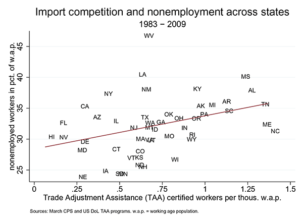
This dataset sheds new light on foreign competition and labor markets outcomes. Figure 1 illustrates a positive relationship between trade-induced job losses and the average nonemployment rate across states.2 In fact, one extra worker displaced due to foreign competition is associated with an overall employment reduction by two to three workers. The reduced employment rate is found to result from both a rise in job destruction and a fall in job creation, while population adjustments are sluggish. These results are robust to state indicators, time indicators, time-region interaction terms, panel-level autocorrelation, heteroskedasticity and various controls including the widely used import penetration proxies and unionization.
These facts are explained using a trade model with heterogeneous firms and heterogeneous labor markets. At the heart of the model, there are some firms which compete monopolistically (see Dixit and Stiglitz (1977)) and others which head-to-head with their foreign rivals (see Dornbusch et al. (1977) and Bernard et al. (2003)).3
In adding segmented locations, the main goal is to have variation in exposure to foreign competition. In the Ricardian tradition, this is accomplished via exogenous firm productivity differences across locations: locations differ in the productivity of their firms.4 Local nonemployment is obtained using random Leontief matching within each labor market and collective Nash bargaining. Workers direct their search and are allocated such that they are indifferent among these locations ex ante.5 Following an unexpected trade reform, consistent with the data, workers can switch firms within their home labor markets but they cannot change location.6
Both cross-sectional productivity differences and variable markups are crucial to explain the correlations between trade, and nonemployment across locations. After a trade reform, firms in the less productive areas face fiercer foreign competition and have more job losses because many of their local firms shut down. These firms shut down because their markups are already compressed and they cannot further reduce them to stave off competition. Fewer jobs are created in the least productive areas because their firms are less likely to outcompete foreign rivals and become new exporters. Hence, the most vulnerable locations have both a higher job destruction rate and a lower job creation rate.
In this model, more productive cities have larger firms, higher population, pay higher wages, and experience higher unemployment rates in the long run. In the long run, the least productive areas simply become ghost towns as their population vanish. In the medium run, when workers can switch employers but not locations, unemployment rates sharply rise in the least productive locations. The productivity channel is further corroborated using state productivity data from Turner et al. (2007) and Turner et al. (2008).
Trade liberalization yields aggregate welfare gains along with large reductions in employment rate and earnings in the badly hit labor markets, when population adjustments are sluggish. This is because the ex ante spatial equilibrium ensures that most firms can tap into their local unemployment pool. However, these aggregate welfare gains do not hold following an unexpected rise in foreign productivity because even the most productive locations are adversely affected.
This paper contributes to a growing literature at the nexus of international trade and labor economics. Topel (1986) and Blanchard and Katz (1992) made influential contributions on differential labor market dynamics across locations and workers. Topalova (2007) and Kovak (2013) study the impact of trade liberalization on migration and wages in India and Brazil respectively.7 Autor et al. (2013b) and Ebenstein et al. (forthcoming) conduct a thorough analysis of U.S. labor markets and trade. They document the worsening of labor market outcomes in localities and occupations that are more exposed to import competition due to their industrial composition.8 This paper extends these findings using geographic data on trade-induced displacements and job flows in the U.S.
Davidson et al. (1999) made a seminal contribution by considering labor search and matching frictions in international trade theory.9 Kambourov (2009), Artuç et al. (2010), Ritter (2012), Cosar (2013), and Dix-Carneiro (2013) recently studied transition paths in dynamic models of trade and unemployment with sectoral and human capital heterogeneity. These models assume that autoworkers at the General Motors factories in Flint, MI are in the same labor market as the autoworkers at the Ford factories in Louisville, KY. This paper introduces a trade and unemployment model with cross sectional productivity differences and geographically segmented labor markets.
This paper is closely related to Beaudry et al. (2012) who estimate a spatial equilibrium model with unemployment in which locations vary in industrial composition. This paper features a trade model in which productivity differences across locations and endogenous variable markups are crucial to account for the uneven effects of foreign competition on unemployment across labor markets.10
This paper is structured as follows. Section 2 empirically analyzes foreign competition and labor market outcomes acrossthe United States using the Trade Adjustment Assistance (TAA) petitions data. Section 3 develops a baseline trade and unemployment model with endogenous variable markups and heterogeneous segmented labor markets. Section 4 conducts two experiments: an unexpected trade reform as well as an unexpected increase in foreign productivity when mobility is limited. Section 5 concludes.
2 Evidence
This section presents the main empirical findings on foreign competition and labor market outcomes across locations. The dataset is based on establishment-level petitions from the U.S. Trade Adjustment Assistance (TAA), individual-level data from Current Population Survey (CPS), job flows data in U.S. Census Business Dynamics Statistics (BDS), housing starts from U.S. Census New Residential Construction (NRC) database, and U.S. imports data combined with U.S. Census County Business Patterns (CBP). The data is aggregated yearly at the state level from 1983 to 2009 into a state-level panel dataset.11
2.2 The Trade Adjustment Assistance (TAA) Petitions Data
Instated in its current form as part of the Trade Act of 1974, the Trade Adjustment Assistance (TAA) for workers is a federal program that aims to support the professional transition of workers displaced due to foreign trade. Each petition includes information on the location of the establishment, the numbers of workers affected, the certification decision, and the date of impact.12
Firms, unions, state unemployment agencies, or groups of workers can file a petition on behalf of a subset of workers at a given establishment. To establish the eligibility of the petitioning workers, federal investigators at the Department of Labor seek evidence that these workers were separated because of (a) import competition that led to decline in sales or production, (b) a shift in production to another country with which the United States has a trade agreement, or (c) due to loss of business as an upstream supplier or downstream producer for another producer that is TAA-certified. Certified workers are eligible to receive benefits such as training, income support, job search allowances, relocation allowances, and healthcare assistance for up to two years.13
For each petition, federal investigators issue a "confidential data request" (CDR) for data such as sales history, sales of import-competing products, major declining customers and unsuccessful bids. The Trade Adjustment Assistance (TAA) investigators also have legal power to issue subpoenas if the company does not comply to the data request.14
2.2 Measuring Foreign Competition
For every year
![]() and for every state
and for every state ![]() in
the U.S., import competition is measured as the ratio of all workers
newly certified for Trade Adjustment Assistance (TAA) relative to
the working age population (w.a.p.):
in
the U.S., import competition is measured as the ratio of all workers
newly certified for Trade Adjustment Assistance (TAA) relative to
the working age population (w.a.p.):
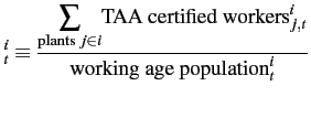
Table1 and Figure 1 show the typical order of magnitude of this TAA-based measure across states between 1983 and 2009. In 2009, a record 330,906 workers were certified for Trade Adjustment Assistance (TAA) across all states.15
Table 1: Summary Statistics (1983-2009)
| p10 | p25 | p50 | p75 | p90 | |
|---|---|---|---|---|---|
| TAA certified workers (per thousand working age population) | 0.03 | 0.17 | 0.43 | 0.88 | 1.64 |
| TAA petitioning workers (per thousand working age population) | 0.11 | 0.39 | 0.80 | 1.43 | 2.38 |
| Unemployed minus US average (percent working age population) | -2.24 | -1.33 | -0.35 | 0.79 | 1.99 |
In contrast, the standard import penetration proxies implicitly assume that two locations producing toys in the U.S. are equally impacted by the imports of toys from China. For example, the measure used in Autor et al. (2013b) - henceforth ADH - is a weighted average of national imports using the local industry mix:

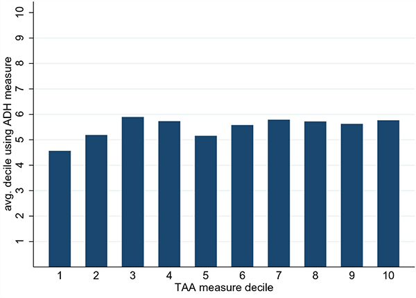
Figure 2 clearly illustrates a weak positive correlation between the standard import penetration proxy and the TAA-based measure, using within-year deciles across states of each variable. Unlike import penetration proxies, the TAA-based measure is direct and it can capture cross-sectional productivity differences between a hypothetical GM auto city and a hypothetical Ford auto city.16
Figure 2: State-Level Import Penetration and TAA-Based Measure
2.3 Foreign Competition and Labor Market Outcomes
The regression below is estimated to assess the relation between import competition and labor market outcomes across the U.S.:

The variable "
TAA foreign competition![]() "
is the share of working age workers certified by the Trade Adjustment
Assistance (TAA) in state
"
is the share of working age workers certified by the Trade Adjustment
Assistance (TAA) in state
![]() during year
during year
![]() .
The variables used as "
labor market outcome
.
The variables used as "
labor market outcome![]() "
are : (a) the share "
not employed
"
are : (a) the share "
not employed![]() "
of working age population workers who are not employed in state
"
of working age population workers who are not employed in state
![]() as of the March CPS of the following year
as of the March CPS of the following year
![]() ;
(b) the rate "
job destruction rate
;
(b) the rate "
job destruction rate![]() "
at which existing jobs were destroyed in state
"
at which existing jobs were destroyed in state
![]() during
year
during
year
![]() ; (c) the rate "
job creation rate
; (c) the rate "
job creation rate![]() "
at which new jobs were created in state
"
at which new jobs were created in state
![]() during year
during year
![]() ; (d) the share "
pop. share
; (d) the share "
pop. share![]() "
of national working age population residing in state
"
of national working age population residing in state
![]() as of the March CPS in
as of the March CPS in
![]() .17
.17
The set of controls
![]() includes the lagged
"
labor market outcome
includes the lagged
"
labor market outcome![]() ", the
lagged "
foreign competition
", the
lagged "
foreign competition![]() ",
the share of working age workers denied by the Trade Adjustment Assistance
(TAA), state indicators, year indicators, year and U.S. Census region
indicators, the state
",
the share of working age workers denied by the Trade Adjustment Assistance
(TAA), state indicators, year indicators, year and U.S. Census region
indicators, the state ![]() income per working age population, the
state share of U.S. working age population. Additional controls include
the state import penetration, the state unionization rate, the state
Trade Adjustment Assistance (TAA) approval rate, the state new housing
units started per working age population. The baseline sample is
a balanced panel of 50 states spanning 27 years from 1983 and
2009.
income per working age population, the
state share of U.S. working age population. Additional controls include
the state import penetration, the state unionization rate, the state
Trade Adjustment Assistance (TAA) approval rate, the state new housing
units started per working age population. The baseline sample is
a balanced panel of 50 states spanning 27 years from 1983 and
2009.
The estimation results are reported in Table 2. Increased foreign competition is correlated with reduced employment through higher job destruction and lower job creation, while population dynamics are sluggish.18 In fact, an extra worker separated (or at risk of being separated) due to foreign competition is associated with the overall employment falling by two to three extra workers relative to other locations.
Naturally, one would be concerned about the ability of the Trade Adjustment Assistance (TAA) federal investigators to identify trade-induced displaced. First, if the TAA investigators were just using industry-level data, the import penetration proxy should be strongly correlated with the TAA measure. This does not appear to be the case as reported in Table 2 and in Figure 2. Furthermore, denied applications or approval rates are not associated with worsening or improving labor market conditions.19
Table 2: Labor Market Outcomes Panel Estimation Across the United States
| Labor market outcomes -> | Not Employed: a1 | Not Employed: a2 | Not Employed: a3 | Job Destruction Rate: b1 | Job Destruction Rate: b3 | Job Creation Rate: c1 | Job Creation Rate: c3 | Population: d1 | Population: d3 |
|---|---|---|---|---|---|---|---|---|---|
| Foreign Competition Variables: TAA Certified Workers | 2.729*** (.544) | - - | 2.792*** (.873) | 1.523** (.697) | 2.443*** (.529) | -1.517*** (.546) | -1.985** (.845) | .508 (1.451) | 0.181 (1.901) |
| Foreign Competition Variables: ADH Import Penetration | - | 0.00135 (.00082) | 0.0007 (.0008) | - - | 0.0006 (.0005) | - - | 0.0008* (.0005) | - - | 0.0005 (.0020) |
| Additional Controls: TAA Denied Workers | 0.644 (.718) | - - | -0.130 (1.052) | 1.240 (.797) | 0.574 (1.016) | 1.200 (.490) | 0.106 (.831) | -0.691 (2.061) | -4.778 (3.160) |
| Additional Controls: New Housing Starts | - - | - - | -1.178*** (.555) | - - | -0.936 (.597) | - - | 0.950 (.769) | - - | 6.965** (3.124) |
| Additional Controls: Unionization Rate | - - | - - | -0.393*** (.051) | - - | 0.015 (.036) | - - | -0.027 (0.46) | - - | -0.131 (.122) |
| Standard Controls: Lagged outcome | Yes | Yes | Yes | Yes | Yes | Yes | Yes | Yes | Yes |
| Standard Controls: Lagged foreign competition | Yes | Yes | Yes | Yes | Yes | Yes | Yes | Yes | Yes |
| Standard Controls: Income (log) | Yes | Yes | Yes | Yes | Yes | Yes | Yes | Yes | Yes |
| Standard Controls: U.S. population share | Yes | Yes | Yes | Yes | Yes | Yes | Yes | - | - |
| Standard Controls: Year indicators | Yes | Yes | Yes | Yes | Yes | Yes | Yes | Yes | Yes |
| Standard Controls: State indicators | Yes | Yes | Yes | Yes | Yes | Yes | Yes | Yes | Yes |
| Standard Controls: Year x Region indicators | Yes | Yes | Yes | Yes | Yes | Yes | Yes | Yes | Yes |
| R-sq. | 0.4466 | 0.5052 | 0.5161 | 0.3689 | 0.2261 | 0.3600 | 0.1629 | 0.9994 | 0.9938 |
| N | 1350 | 750 | 750 | 1350 | 750 | 1350 | 750 | 1350 | 750 |
Note: *, **, and *** denote significance at the 10, 5, and 1 percent level. Robust standard errors in parentheses are clustered on states. The estimation sample is a balanced panel of the 50 states that spans 27 years from 1983 and 2009. Union data is only available after 1989 in the March CPS. Import penetration can only be constructed between 1988 and 2005 with a gap in 1998 to a change from SIC to NAICS.
The findings reported do not hold when the import penetration proxy is used instead of the direct TAA measure, as shown in the specification (a2) of Table 2. The findings for the direct measure based on the Trade Adjustment Assistance (TAA) still hold after controlling for the import penetration proxy as shown in the specifications (a3), (b3), (c3), and (d3) of Table 2.20 The results are robust to controlling for unionization rates as well as local spillovers in the non-tradable sector using housing starts data.
These findings reported above pose a challenge to existing models. Certainly, models with frictionless or centralized labor markets are not equipped to replicate these results and address related questions: why does foreign competition have a correlated effect of both job destruction and job creation? what are the consequences of the limited geographical mobility of workers in response to trade shocks? what are the welfare effects of the uneven effect of foreign competition across locations? These questions are addressed using a Ricardian model with heterogeneous firms, variable markups, and segmented labor markets.
3 Trade Model with Segmented Labor Markets
3.1 Environment
The baseline environment consists of two symmetric countries ![]() populated by a unit measure of families and firms.21 Each family is composed of
populated by a unit measure of families and firms.21 Each family is composed of ![]() individuals allocated across a continuum
of locations in their country. These locations vary in the exogenous
productivity of their local firms. Within a given location, local
firms vary in the degree of foreign competition they face. Local nonemployment
is obtained using random Leontief matching of workers to firms and
collective Nash bargaining. The population distribution is determined
by the uncoordinated search for work across locations. There are international
iceberg transportation costs
individuals allocated across a continuum
of locations in their country. These locations vary in the exogenous
productivity of their local firms. Within a given location, local
firms vary in the degree of foreign competition they face. Local nonemployment
is obtained using random Leontief matching of workers to firms and
collective Nash bargaining. The population distribution is determined
by the uncoordinated search for work across locations. There are international
iceberg transportation costs ![]() .22
.22
Preferences
Following Helpman and Itskhoki (2010), each family has quasi-linear
preferences over its homogeneous good consumption ![]() and its
composite good consumption
and its
composite good consumption ![]() :
:
![]() ,
where
,
where ![]() is a Spence-Dixit-Stiglitz aggregator over differentiated
goods:
is a Spence-Dixit-Stiglitz aggregator over differentiated
goods:

and
![]() .
.
Figure 3: A Simple Overview of the Model
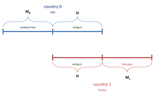
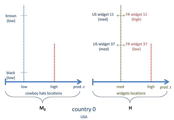
The differentiated goods have two possible types, monopolistic
or head-to-head, as illustrated in Figure 3.
The monopolistic goods ("![]() goods") have no foreign counterpart
and the producers of these goods are monopolistic competitors (e.g.
American cowboy hat varieties and French foie gras varieties in the
illustration). The head-to-head ("
goods") have no foreign counterpart
and the producers of these goods are monopolistic competitors (e.g.
American cowboy hat varieties and French foie gras varieties in the
illustration). The head-to-head ("![]() goods") each have a domestic
counterpart and a foreign counterpart that are perfect substitutes
(e.g. widget varieties in the illustration).
goods") each have a domestic
counterpart and a foreign counterpart that are perfect substitutes
(e.g. widget varieties in the illustration).
Taking the homogeneous good as numeraire, a household in country
![]() faces a composite good price index
faces a composite good price index ![]() defined as:
defined as:
 .
A household with total income
 ![]() from earnings and profits optimally
chooses:
from earnings and profits optimally
chooses:

where
![]() .
.
Technology and Competition
Each ![]() type producer is a monopolistic competitor. Each
type producer is a monopolistic competitor. Each ![]() type
producer competes via simultaneous price setting against a unique
foreign counterpart.23
type
producer competes via simultaneous price setting against a unique
foreign counterpart.23
A model that includes only monopolistic competitors without direct foreign competition will fail to match the data simply because it cannot generate job losses due to foreign competition. A model without monopolistic competitors, on the other hand, may overstate the effects of foreign competition on job losses and understate the gains from increased varieties.
An exogenous measure ![]() of firms can produce (head-to-head)
of firms can produce (head-to-head) ![]() goods
and the remaining measure
goods
and the remaining measure ![]() can produce (monopolistic)
can produce (monopolistic) ![]() goods.
There is a fixed unit measure of differentiated varieties (and firms)
in each country. There are no fixed costs of entry or operation. The
model is therefore a hybrid setup combining Chamberlinian monopolistic
competition with head-to-head imperfect competition. These two modes
of competition are special cases (
goods.
There is a fixed unit measure of differentiated varieties (and firms)
in each country. There are no fixed costs of entry or operation. The
model is therefore a hybrid setup combining Chamberlinian monopolistic
competition with head-to-head imperfect competition. These two modes
of competition are special cases (![]() and
and ![]() respectively).24
respectively).24
Each firm ![]() is exogenously assigned its variety
is exogenously assigned its variety
![]() and its productivity
and its productivity
![]() . Each head-to-head producer
also has a randomly assigned foreign competitor. Each firm
. Each head-to-head producer
also has a randomly assigned foreign competitor. Each firm ![]() can produce its differentiated good
can produce its differentiated good
![]() using
a linear production technology:
using
a linear production technology:
where ![]() is the labor input and
is the labor input and ![]() is the output.
The productivity
is the output.
The productivity
![]() is assumed to be drawn randomly from
a Pareto distribution with lower bound
is assumed to be drawn randomly from
a Pareto distribution with lower bound ![]() and shape parameter
and shape parameter
![]() :
:
![]() .
.
The firms in the homogeneous good sector are homogeneous, compete
perfectly and have a simple linear technology:
![]() .
.
Heterogeneous Locations and Segmented Labor Markets
The main goal in defining locations is to have variations in foreign
competition. In the Ricardian tradition, a labor market is defined
such that all the firms in that location share the same productivity
level (![]() ) and the same type (
) and the same type (![]() or
or ![]() ).25 Therefore, in each country, there are many
).25 Therefore, in each country, there are many ![]() type (head-to-head)
towns and many
type (head-to-head)
towns and many ![]() type (monopolist) towns, in addition to homogeneous
good towns.26
type (monopolist) towns, in addition to homogeneous
good towns.26
There is still heterogeneity across firms within each ![]() type (head-to-head)
town even though they share the same productivity. Figure 4 provides an illustration of these differences across and within locations.
Firms collocated in the same
type (head-to-head)
town even though they share the same productivity. Figure 4 provides an illustration of these differences across and within locations.
Firms collocated in the same ![]() type (head-to-head) town share the
same productivity. Yet, they differ in their varieties and in the
productivity of their head-to-head foreign competitors. Within an
type (head-to-head) town share the
same productivity. Yet, they differ in their varieties and in the
productivity of their head-to-head foreign competitors. Within an
![]() type (monopolist) town, firms share the same productivity and
they each produce different varieties.27
type (monopolist) town, firms share the same productivity and
they each produce different varieties.27
Figure 4: A Simple Illustration of Locations
The economy is composed of a continuum of labor markets across which families assign their workers. Within each local labor market, workers are randomly matched with vacancies based on a Leontief matching function: firms fill all their vacancies as long as there are more workers looking for jobs than vacancies.28
At each plant, the workers bargain collectively with the firm over
wages and production decisions.29 The workers collectively have bargaining power ![]() .30 Firms have to pay a hiring cost
.30 Firms have to pay a hiring cost ![]() per hire. The union's threat
point is defined by a home production technology yielding
per hire. The union's threat
point is defined by a home production technology yielding ![]() units
of the numeraire good. It is convenient to interchangeably identify
a plant with productivity
units
of the numeraire good. It is convenient to interchangeably identify
a plant with productivity ![]() by:
by:
Finally, the homogeneous sector is subject to no hiring or matching frictions.
3.2 Characterization
The Monopolist ( type) Firm Problem
Consider a monopolist firm in country ![]() with productivity
with productivity ![]() and supplying country
and supplying country ![]() . With
. With
![]() workers, the firm-union
match generates the following surplus:
workers, the firm-union
match generates the following surplus:
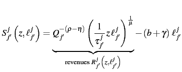
The firm's profit from this plant is:
 where
where
![]() is the wage paid to the workers.
The wages
is the wage paid to the workers.
The wages
![]() and the plant size
and the plant size
![]() are determined through Nash-bargaining with the workers' union by
solving:31
are determined through Nash-bargaining with the workers' union by
solving:31
![$\displaystyle \max_{w,\ell}\left[Q_{j'}^{-\left(\rho-\eta\right)}\left(\frac{1}{\tau_{j'}^{j}}\, z\,\ell\right)^{\frac{1}{\mu}}-\gamma\,\ell-w\,\ell\right]^{1-\lambda}\cdot\,\,\left[\left(w-b\right)\,\ell\right]^{\lambda}
$](img98.gif)
Since all costs are variable, the optimal outcome splits the maximal net surplus according to the bargaining power. Hence, the firm-union produces the monopolistic output and proportionally splits the net surplus generated. That is:
![\begin{displaymath}
\begin{array}{lll}
p_{j'}^{j}\left(c\right) & =\mu\,\tau_{j'}^{j}\, c\\
w_{j'}^{j}\left(c\right)-b & =\lambda\left(\mu-1\right)\,\left(\gamma+b\right) & \equiv w_{M}-b\\
\ell_{j'}^{j}\left(c\right) & =Q_{j'}^{-\frac{\rho-\eta}{1-\rho}}\,\Big[\mu\,\left(\gamma+b\right)\Big]^{-\sigma}\,\left[\,\,\dfrac{\left(\gamma+b\right)}{\tau_{j'}^{j}\,\, c}\,\,\right]^{\sigma-1} & \equiv\mu^{-\sigma}\,\overline{\ell}_{j'}^{j}\left(c\right)
\end{array}\end{displaymath}](img99.gif)
where
![]() is the firm-union unit cost and
is the firm-union unit cost and
 is the size corresponding to the marginal cost pricing (zero profits).
The ![]() type (monopolist) producers therefore choose the standard
markup pricing rule that equalizes the marginal revenue and the marginal
cost. Although more productive firms are larger, it is important to
note that the wages are independent of the firm productivity. This
has been a standard result in environments with power revenue functions
and linear technology.32 This property that wages do not depend on firm productivity implies
that the
type (monopolist) producers therefore choose the standard
markup pricing rule that equalizes the marginal revenue and the marginal
cost. Although more productive firms are larger, it is important to
note that the wages are independent of the firm productivity. This
has been a standard result in environments with power revenue functions
and linear technology.32 This property that wages do not depend on firm productivity implies
that the ![]() type (monopolist) towns the same wage and therefore
the same equilibrium employment rate. Each worker extracts a share
type (monopolist) towns the same wage and therefore
the same equilibrium employment rate. Each worker extracts a share
![]() of the net markup
of the net markup
![]() . Also, since there
are no fixed cost of exporting, all
. Also, since there
are no fixed cost of exporting, all ![]() type producers export in
this model.
type producers export in
this model.
Employment Rates
Finally, given the random Leontief matching, an ![]() type labor
market of firms with productivity
type labor
market of firms with productivity ![]() has an employment rate
has an employment rate ![]() :
:

where ![]() is the endogenous population of workers
available in that town. The expected earnings per worker
W
is the endogenous population of workers
available in that town. The expected earnings per worker
W![]() in the town of an
in the town of an ![]() type producer with productivity
type producer with productivity ![]() therefore
satisfy:
W
therefore
satisfy:
W![]() .
.
The Head-to-Head ( type) Firm Problem
Consider a head-to-head firm in country ![]() that is hiring
that is hiring
![]() workers to supply country
workers to supply country ![]() . Let
. Let ![]() be the firm's productivity
and
be the firm's productivity
and ![]() be its foreign competitor's productivity. Unlike
a monopolistic firm, the firm has to set its price above its competitor's
zero profit price (see Bernard et al. (2003)). The firm therefore solves:
be its foreign competitor's productivity. Unlike
a monopolistic firm, the firm has to set its price above its competitor's
zero profit price (see Bernard et al. (2003)). The firm therefore solves:
![\begin{displaymath}
\begin{array}{ll}
{\displaystyle \max_{w,\ell}} & \left[Q_{j'}^{-\left(\rho-\eta\right)}\left(\frac{1}{\tau_{j'}^{j}}\, z\,\ell\right)^{\frac{1}{\mu}}-\gamma\,\ell-w\,\ell\right]^{1-\lambda}\cdot\,\,\left[\left(w-b\right)\,\ell\right]^{\lambda}\\
\qquad\text{s.t.}\\
& p_{j'}^{j}\left(z,\ell\right)\leq\overline{p}_{j'}^{1-j}\left(\tilde{z}\right)\\
& \pi_{j'}^{j}\left(z,\ell\right)\ge0
\end{array}\end{displaymath}](img122.gif)
where
![]() is the foreign competitor's marginal cost to supply country
is the foreign competitor's marginal cost to supply country ![]() .
.
Due to head-to-head competition, this ![]() type producer from country
type producer from country
![]() supplies a country
supplies a country ![]() if and only if it is the lowest unit
cost supplier for that market:
if and only if it is the lowest unit
cost supplier for that market:
![]() .
Conditional on supplying the market
.
Conditional on supplying the market ![]() , the producer may either
be at the corner (constrained) or choose the unconstrained monopolistic
(constant markup) price:
, the producer may either
be at the corner (constrained) or choose the unconstrained monopolistic
(constant markup) price:
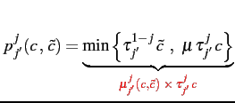
The threat of being undercut induces variable markups
![]() as the firm seeks to maximize the net surplus shared with its workers.
Less productive firms are more likely to have lower markups as they
are more likely to face more productive competitors.
as the firm seeks to maximize the net surplus shared with its workers.
Less productive firms are more likely to have lower markups as they
are more likely to face more productive competitors.
Given the net surplus sharing outcome, wages are commensurate to the variable markup:

Therefore, wages are variable in contrast to the case of the monopolistic firms that do not face head-to-head competition. Less productive firms are also more likely to pay lower wages due to lower markups. Also, the more productive the competitor faced, the larger the firm because the lower markup translates into a higher demand and lower markups:
![$\displaystyle \ell_{j'}^{j}\left(c\,,\,\tilde{c}\right)=\Big[{\color{red}\mu_{j'}^{j}\left(c,\tilde{c}\right)}\Big]^{-\sigma}\times\overline{\ell}_{j'}^{j}\left(c\right)
$](img133.gif)
The effect of the head-to-head competition on the firm behavior also
depends on the level of frictions to international trade. In fact,
as the tariff ![]() goes to infinity (autarky), the
goes to infinity (autarky), the ![]() type producers
are all in operation and they all charge the unconstrained monopolistic
price:
type producers
are all in operation and they all charge the unconstrained monopolistic
price:
![]() .
On the other hand, when trade is frictionless, only some firms charge
the monopolistic price.33
.
On the other hand, when trade is frictionless, only some firms charge
the monopolistic price.33
Figure 5: Variable Markups Across Firms and Locations
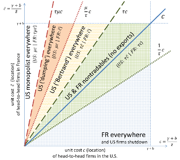
The model therefore generates rich pricing-to-market markups as shown
in Figure 5.
34 A point
![]() represents a head-to-head firm
located in a town of productivity
represents a head-to-head firm
located in a town of productivity
![]() and facing a competitor with productivity
and facing a competitor with productivity
![]() .
Hence, a vertical line represents a head-to-head town of productivity
.
Hence, a vertical line represents a head-to-head town of productivity
![]() .
.
These variable markups are also the reason why productivity differences yield differences in foreign competition across locations: in the more productive locations, more firms outcompete their foreign competitors relative to the less productive locations. Hence, in less productive locations, more firms do not produce but shutdown altogether (see blue solid diamond region in Figure 5). Also, firms from less productive locations are more likely to produce without exporting. This region is akin to the Ricardian non-tradable region and yields an extensive margin of new exporters when trade barriers fall (see green gridded region in Figure 5).
The model also generates a region of international "dumping": firms charge the monopolistic price at home and the competitor's marginal cost abroad (see solid colored region in Figure 5). This outcome could suggest "dumping" since the ratio of prices at home and abroad is larger than the iceberg transportation costs. This "dumping" region only disappears in the limit case of frictionless trade.35
Employment Rates
Based on these results, a town of ![]() type (head-to-head) producers
with productivity
type (head-to-head) producers
with productivity ![]() has an employment rate
has an employment rate ![]() satisfying:
satisfying:
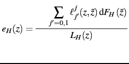
where ![]() is the endogenous population of the town
and
is the endogenous population of the town
and
![]() if a producer is outcompeted.
The expected earnings per worker
W
if a producer is outcompeted.
The expected earnings per worker
W![]() in
that town satisfy:
in
that town satisfy:
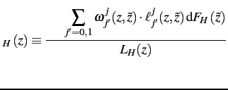
Labor Allocation Across Locations
Workers are allocated knowing the tariff, the town's type (monopolistic
or head-to-head competition), and the local productivity. So, each
family knows the distribution of wages and nonemployment rates across
towns. Each family therefore allocates
![]() such that:
such that:

In equilibrium, families must be indifferent across locations to send workers.
Market Clearing
The market clearing condition for each differentiated good is trivially satisfied. Since hiring costs are paid in units of the homogeneous good, its market clearing condition is:

3.3 Equilibrium
A symmetric equilibrium with tariff ![]() is: (a) a price index
is: (a) a price index
![]() ; (b) quantities
; (b) quantities ![]() and
and ![]() ; (c) aggregate earnings W;
(d) aggregate profits
; (c) aggregate earnings W;
(d) aggregate profits ![]() ; (e) populations
; (e) populations
![]() such that: (i) households solve their utility maximization given prices,
profits and earnings; (ii) firms producing the differentiated goods
solve their profit maximization problem given their productivity,
their competition, and the aggregate consumption indexes; (iii) aggregate
profits, aggregate earnings, and the price index are consistent with
the firm decisions; (iv) all goods markets clear; and (v) the indifference
condition across towns for labor allocation holds.
such that: (i) households solve their utility maximization given prices,
profits and earnings; (ii) firms producing the differentiated goods
solve their profit maximization problem given their productivity,
their competition, and the aggregate consumption indexes; (iii) aggregate
profits, aggregate earnings, and the price index are consistent with
the firm decisions; (iv) all goods markets clear; and (v) the indifference
condition across towns for labor allocation holds.
3.4 Wages and Nonemployment Across Locations
The following properties hold in equilibrium.36
Proposition 1. Equal expected earnings.
Expected earnings are equalized across all labor markets. Average income is also equalized across locations since all workers receive an equal share of firm profits.
Proof. The proposition trivially follows from the labor allocation indifference condition. Given the quasi-linear preferences, the equilibrium indifference condition means that expected earnings are equalized across locations:37

where
![]() is the wage in the homogeneous regions.
is the wage in the homogeneous regions.
In light of this proposition, greater vulnerability to foreign competition due to lower productivity does not necessarily mean that labor market outcomes are worse ex ante. Moreover, ex ante, no transfers are required across locations to equate consumption allocations because the indifference condition makes it trivial. In others words, ex ante, transfers within a location are enough to implement the optimal consumption allocation for each individual.
Proposition 2. Constant nonemployment rate across monopolistic locations.
Across monopolistic locations, more productive labor markets have higher total employment and population but workers earn the same wage and face the same nonemployment rate as less productive monopolistic locations.
Proof. The proof is based on Proposition 1 and the optimal firm decision. Wages are constant across monopolistic locations because markups are constant and the bargaining yields a simple net surplus sharing rule.
This proposition is important because it shows why, in this class of models, head-to-head competition can induce a non-degenerate distribution of employment rates across labor markets. In the absence of head-to-head competition, the distribution of nonemployment rate is degenerate because wages would be independent of firm productivity. Consequently, the wage determination rule assumed in this class of models or the constant markups are innocuous assumptions. However, the abstraction from multilateral bargaining is not problematic as long as the constant wage and proportional net surplus sharing results hold. This is the case in Helpman and Itskhoki (2010) and Felbermayr et al. (2010) for example.
Proposition 3. Different nonemployment rates across head-to-head locations.
Across head-to-head locations, when there are no trade barriers, the more productive labor markets have higher employment, pay higher wages and thereby have higher nonemployment rate than less productive labor markets.
Proof. The proof follows from Proposition 1 and the fact that expected markups and wages in head-to-head locations increase with local productivity.
This proposition characterizes the free trade long run equilibrium.38 In the extreme case of autarky, the distribution of markups and employment
rates become degenerate since
![]() . In
general, trade barriers (
. In
general, trade barriers (![]() ) interact with the ideal markup (
) interact with the ideal markup (![]() )
to alter the entire distribution of markups as illustrated in Figure 5. Hence, the expected markups across head-to-head
locations do not always fall with productivity.
)
to alter the entire distribution of markups as illustrated in Figure 5. Hence, the expected markups across head-to-head
locations do not always fall with productivity.
3.5 Equilibrium Labor Allocations
The employment rate across monopolistic locations is degenerate and corresponds to the employment rate of the most productive head-to-head locations. On the other hand, the endogenous distribution of variable markups across locations also corresponds to a distribution of employment rates.
Figure 6: Trade Barriers and Employment Rate
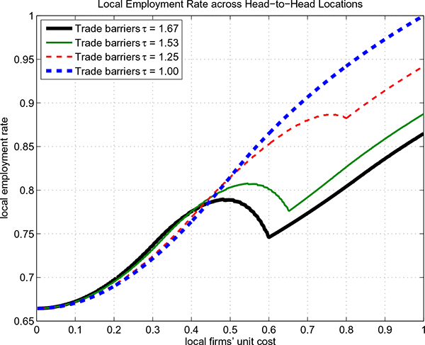
Figure 6 shows the equilibrium employment-to-population across head-to-head labor markets for various levels of trade barriers.39 By Proposition 3, in the absence of trade barriers, the nonemployment rate across head-to-head locations decreases with productivity. However, the monotonicity does not hold in the presence of trade barriers. First, there is a kink at the marginal productivity level where all firms in a head-to-head location do not export. Above the kink, a slightly less productive location has a higher employment rate because it faces tougher competition. Below the kink, the infra-marginal location exports and has a higher employment rate because trade costs lower markups abroad. Eventually, more productive locations have more firms charging higher markups. Therefore, the hump is an artifact of the changing composition of the endogenous markups. The kink and the hump naturally vanish in the absence of trade costs. Furthermore, the model predicts that more productive locations have higher employment level since their firms are larger.
3.6 Long-Run Reallocation Across Labor Markets
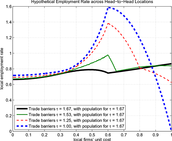
When workers are mobile within and across labor markets, the most affected locations become ghost towns in the free trade equilibrium: their population vanish. As shown in Figure 7, some labor markets greatly expand and employ more workers than their original population.40 However, the full mobility assumption is at odds with the empirical evidence on muted population adjustments to trade shocks. Therefore, in the next section, worker mobility after a trade reform shock is restricted.
Figure 7: Reallocation of Labor with Full Mobility
4 Unexpected Trade Reform with Limited Mobility
Consistent with the muted population adjustments in the data, workers are now assumed to be ex ante mobile across labor markets but not ex post as in Helpman and Itskhoki (2010). The ex post immobility assumption means that workers cannot leave their original home locations even though they may switch jobs.
The ex ante indifference condition across locations no longer has to hold ex post. Labor markets may still expand by tapping into their local pool of nonemployed workers. An equilibrium with limited worker mobility is defined below. The model is calibrated to study trade-induced labor market adjustments across locations.
4.1 Medium Run Equilibrium Post-Reform
Given an initial equilibrium population allocation
![]() with tariff
with tariff ![]() , a symmetric medium run equilibrium with
tariff
, a symmetric medium run equilibrium with
tariff
![]() is: (a) a price index
is: (a) a price index
![]() ; (b)
quantities
; (b)
quantities
![]() and
and
![]() ; (c) earnings
; (c) earnings
![]() ;
and (e) aggregate profits
;
and (e) aggregate profits
![]() such that: (i) households
solve their utility maximization problem; (ii) firms solve their profit
maximization problems; (iii) aggregate profits, aggregate earnings,
employment rates, and the price index are consistent; (iv) all goods
markets clear.
such that: (i) households
solve their utility maximization problem; (ii) firms solve their profit
maximization problems; (iii) aggregate profits, aggregate earnings,
employment rates, and the price index are consistent; (iv) all goods
markets clear.
4.2 Calibration
The limited mobility model is calibrated to quantify the effects
of a trade liberalization across labor markets in the U.S. The
Armington elasticity is set to
![]() following Ruhl (2009).
The iceberg transportation cost before the reform is chosen to be
in the range of trade costs - including observed tariffs and non-tariff
barriers - documented by Anderson and van Wincoop (2004) for the U.S.
following Ruhl (2009).
The iceberg transportation cost before the reform is chosen to be
in the range of trade costs - including observed tariffs and non-tariff
barriers - documented by Anderson and van Wincoop (2004) for the U.S.
The Pareto distribution shape parameter is set to ![]() to guarantee
finite mean and finite variance, following Helpman and Itskhoki (2010).
The elasticity of substitution with the outside good
to guarantee
finite mean and finite variance, following Helpman and Itskhoki (2010).
The elasticity of substitution with the outside good ![]() is set
to
is set
to
![]() to ensure that varieties are
better substitutes for each other than for the homogeneous good. The
bargaining power
to ensure that varieties are
better substitutes for each other than for the homogeneous good. The
bargaining power ![]() is set to 0.5 so the union and the firm
have equal bargaining power. The fraction of firms subject to head-to-head
foreign competition is chosen so that the average number of trade-induced
displacements matches the data (0.7 workers percent of w.a.p.).
The outside option parameter is chosen so that all local labor markets
attract workers under full worker mobility. The other parameters
are set to have a national nonemployment rate around 30 percent in
free trade. The calibration parameters are summarized in Table 3.
is set to 0.5 so the union and the firm
have equal bargaining power. The fraction of firms subject to head-to-head
foreign competition is chosen so that the average number of trade-induced
displacements matches the data (0.7 workers percent of w.a.p.).
The outside option parameter is chosen so that all local labor markets
attract workers under full worker mobility. The other parameters
are set to have a national nonemployment rate around 30 percent in
free trade. The calibration parameters are summarized in Table 3.
Table 3: Calibration
| Parameter | Description | Value |
|---|---|---|
| H | Fraction of head-to-head firms | 0.01 |
| M | Fraction of monopolist firms | 0.99 |
| σ | Armington elasticity | 2.01 |
| η | Elasticity of substitution of differentiated good | 0.25 |
| s | Pareto distribution shape | 2.05 |
| λ | Union bargaining power | 0.50 |
| b | Outside option | 1.00 |
| γ | Hiring cost | 0.02 |
| L | Population | 1.00 |
| τ | Iceberg transportation costs pre-liberalization | 1.11 |
| Iceberg transportation costs post-liberalization | 1.00 |
4.3 Foreign Competition and Nonemployment
To relate the model to the empirical findings, the import competition faced by a labor market is measured using a statistic akin to Trade Adjustment Assistance (TAA) certifications observed in the data: the number of workers in a given labor market that are displaced because of foreign competition. In the model, this is the fraction of local workers who lost their jobs after their plant shut down due to heightened head-to-head competition. This measure is equal to zero in non head-to-head labor markets.41 Figure 8 illustrates the relationship between the measure of TAA-certified workers and nonemployment changes.
Figure 8: Foreign Competition and Nonemployment
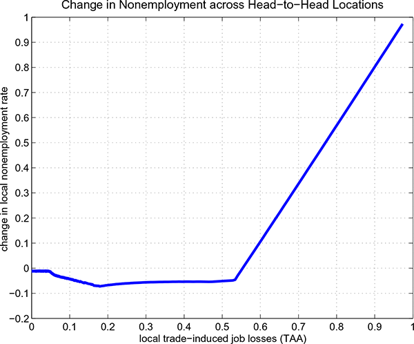
First, net changes in nonemployment maybe positive or negative depending on the productivity of the head-to-head labor markets. As indicated earlier, the non head-to-head labor markets correspond to a degenerate distribution at the point where trade-induced job losses are zero. Second, the reduced job creation explains the increased steepness of the curve in the locations experiencing the largest job destruction. Third, it is easy to observe that the elasticity of local nonemployment to local job losses due to foreign competition is slightly larger than two in the worst hit locations.42 The model therefore suggests that a selection bias in the petition process is needed to generate the measured elasticity of nonemployment to trade-induced displacements.
As trade barriers fall, the firms in the marginal exporting labor markets are able to outcompete their foreign rivals in foreign markets, and thereby expand at the extensive margins. Less productive head-to-head locations lose most of their firms because they are out-competed. At the other extreme, the most productive head-to-head labor markets are hardly affected by the fall in trade barriers as they behave as monopolists. These changes in markups and export participation drive changes labor market outcomes across locations.
The overall relationship for the employment rate is non monotonic due to the heterogeneity in markups and the correlation between lower productivity and vulnerability to import competition.
The relationship is quantitatively and qualitatively robust to the
size of the head-to-head sector (![]() ).43 This is because the size of the head-to-head sector mainly affects
the aggregate price index while the nonlinear effects are driven by
the endogenous changes in variable markups illustrated in Figure 5.
On the other hand, the elasticity of substitution
).43 This is because the size of the head-to-head sector mainly affects
the aggregate price index while the nonlinear effects are driven by
the endogenous changes in variable markups illustrated in Figure 5.
On the other hand, the elasticity of substitution ![]() is key
for the magnitude of the elasticity of nonemployment to trade-induced
displacements.
is key
for the magnitude of the elasticity of nonemployment to trade-induced
displacements.
4.4 Welfare Gains and Limited Worker Mobility
Both the model and the data indicate that import competition has large uneven effects on labor markets across locations. The model predicts overall aggregate welfare gains and increased aggregate employment in the medium run, despite the large increase in nonemployment and the fall in earnings in the worst hit locations. The aggregate effects are summarized in Table 4.
Table 4: Effects of Limited Mobility in the Medium Run
| Trade job losses (per 1,000) | Not employed (percent) | %ΔQ (diff.goods) | %Δq0 (hom. good) | %ΔU (utility) | |
|---|---|---|---|---|---|
| Pre-reform | 0.00 | 30.32 | - | - | - |
| Medium run | 0.70 | 29.28 | +7.02 | -0.25 | +1.69 |
| Long run | 0.00 | 30.84 | +7.03 | -19.51 | +1.37 |
These medium run (limited mobility) welfare gains are actually not smaller than the long run (full mobility) gains. While the differentiated good demand is lower, limited mobility reduces inefficiencies from search frictions by increasing the overall employment level. In this model, the main source of nonemployment is the inefficiency from the directed search as opposed to matching frictions. Hence, limited mobility partially undoes that inefficiency as in Helpman and Itskhoki (2010).
While full labor mobility ensured that earnings were equalized across labor markets, limited mobility induces a non-degenerate distribution of expected earnings. This medium run earnings inequality is a source of income redistribution across labor markets. In contrast, under full worker mobility, no redistribution across labor markets is needed because of the indifference condition.44
Table 5: Labor Market Outcomes Using TFP Estimates Across States
| Labor market outcomes -> | Nonemployed Workers: a4 | Nonemployed Workers: a5 | Nonemployed Workers: a6 | Job Destruction Rate: b4 | Job Destruction Rate: b6 | Job Creation Rate: c4 | Job Creation Rate: c6 | Population: d4 | Population: d6 |
|---|---|---|---|---|---|---|---|---|---|
| Foreign Competition: TAA Certified Workers | 2.819** (1.255) |
- - |
2.625 (1.800) |
1.489** (.682) |
-0.245 (1.017) |
-1.496*** (.531) |
-1.233 (.783) |
0.005 (.015) |
0.016 (.238) |
| Foreign Competition: TAA Certified Workers2 | -65.04 |
- - |
-218.50 (316.17) |
- - |
- - |
- - |
- - |
- - |
- - |
| Total Factor Productivity: Log TFP | - - |
-2.928** (1.320) |
-2.933** (1.324) |
- - |
-0.167*** (.061) |
- - |
0.222*** (.042) |
- - |
0.0005 (.0014) |
| Total Factor Productivity: Log TFP2 | - - |
0.468** (.216) |
-0.469** (.217) |
- - |
- - |
- - |
- - |
- - |
- - |
| Standard Controls: Lagged outcome | Yes |
Yes |
Yes |
Yes |
Yes |
Yes |
Yes |
Yes |
Yes |
| Standard Controls: Lagged independent variables | Yes |
Yes |
Yes |
Yes |
Yes |
Yes |
Yes |
Yes |
Yes |
| Standard Controls: Year indicators | Yes |
Yes |
Yes |
Yes |
Yes |
Yes |
Yes |
Yes |
Yes |
| Standard Controls: State indicators | Yes |
Yes |
Yes |
Yes |
Yes |
Yes |
Yes |
Yes |
Yes |
| Standard Controls: Year x Region indicators | Yes |
Yes |
Yes |
Yes |
Yes |
Yes |
Yes |
Yes |
Yes |
| R-sq. | 0.7388 |
0.6352 |
0.6236 |
0.4925 |
0.6296 |
0.5654 |
0.4377 |
0.9996 |
0.9995 |
| N | 1350 |
900 |
900 |
1350 |
900 |
1350 |
900 |
1350 |
900 |
Note: *, **, and *** denote significance at the 10, 5, and 1 percent level. Robust standard errors in parentheses are clustered on states. The estimation sample is a balanced panel of the 50 states that spans 27 years from 1983 and 2009. State-level TFP estimates are available only up to 2000.
4.5 Evidence using Measured Cross-Sectional Productivity
A fundamental ingredient in this model is the heterogeneity in productivity across locations: differences in trade-induced displacements are due to productivity differences across locations. In particular, the model predicts a nonlinear quadratic relation between productivity and nonemployment when population adjustments are muted.
These key tenants of the model are investigated using state-level data on Total Factor Productivity (TFP) estimated by Turner et al. (2007) and Turner et al. (2008). These TFP estimates are derived using carefully constructed data on state-level sectoral inputs, especially physical capital, human capital, and land. The empirical estimation is similar to the one used in Section 2. The results are shown in Table 5. All the estimated specifications include state indicators, year indicators, year-region indicators, and lagged variables.45
In specifications (a5) and (a6) of Table 5, the nonlinear effects of productivity on nonemployment rate are corroborated. Consistent with the theory, trade-induced displacements are no longer significant when productivity is accounted for in specification (a6). However, the quadratic effect is not significant when the trade-induced displacements alone are used in specification (a4). This finding reinforces the possibility of a selection bias in the petitions as noted above.46
Finally, productivity has a correlated effects on job creation and job destruction. In specifications (b6) and (c6), the less productive locations create fewer new jobs and lose more existing jobs.47 Population dynamics remain muted in response to productivity innovations as shown in specifications (d4) and (d6).
Altogether, these findings reinforce the view that trade reforms unevenly affect locations through preexisting cross-sectional productivity differences.
4.6 Trade Reforms and Exogenous Growth: Similar Effects?
In international trade, a fall in trade barriers and a growth in foreign productivity may have similar effects. For instance, Autor et al. (2013b) argue that the adverse labor market effects of import competition from China are due to exogenous growth in China. In this subsection, the effects of an unexpected trade reform and an exogenous foreign productivity growth in this model are contrasted.
To do so, an asymmetric free trade equilibrium is first computed by extending the symmetric setup in Section 3. The two countries are assumed to be different in their Pareto shape parameter. An unexpected productivity increase is then induced in the spirit of the medium run equilibrium of Section 4. Specifically, the tail parameter in the foreign country is reduced from 2.29 to the home economy's tail parameter: 2.05. This represents a 10 percent growth in average productivity in the differentiated sectors.48
Figure 9: Nonemployment Under Exogenous Foreign Growth
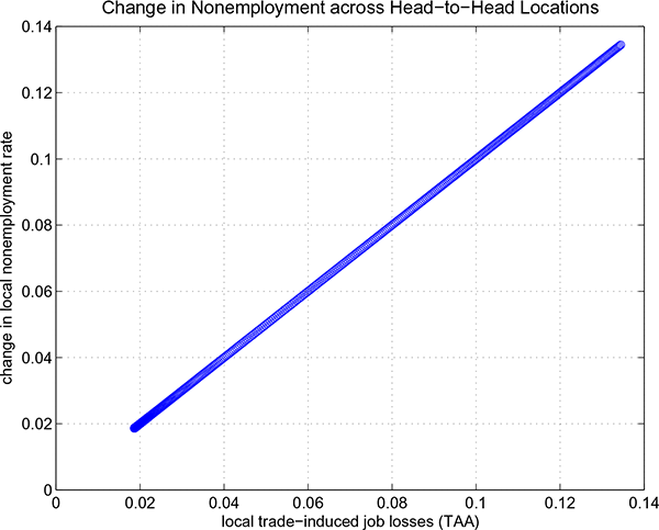
Figure 9 illustrates the net changes in nonemployment and trade-induced job losses across head-to-head labor markets when the foreign and less productive country experiences an exogenous growth in productivity in the absence of trade barriers. There is a systematic contraction across labor markets in the medium run. All domestic labor markets lose jobs due to the surge in foreign competition. Aggregate employment falls across the board as no new jobs are created. Unlike the trade reform case, the relationship is no longer nonlinear and the elasticity of local nonemployment to local job losses due to foreign competition is equal to one everywhere. Overall, these effects yield negative aggregate welfare effects in the advanced economy due to the induced fall in aggregate income.
This exercise shows that, in this model, the labor market effects of trade reforms and foreign productivity are not identical in the cross-section or in the aggregate. Recent studies such as Autor et al. (2013a) have started exploring the identification of technology shocks and trade shocks across locations. This is certainly an important and a complex problem. For instance, in this model, trade openness endogenously amplifies cross-sectional technology differences.
5 Conclusion
This paper studies the labor market effects of trade-induced foreign competition across locations in the U.S. The impact of foreign competition on labor markets is documented using a novel dataset on the universe of establishment-level petitions for Trade Adjustment Assistance (TAA) in the U.S. over the last three decades. Increased foreign competition is correlated with reduced employment through higher job destruction and lower job creation, while population dynamics are sluggish. Across locations, an extra worker separated due to foreign competition is associated with the overall employment falling by two to three extra workers. These findings are robust to location fixed effects, time fixed effects, region and time interactions, import penetration, construction activity, and unionization.
This paper introduces a Ricardian model with nonemployment, variable markups, and heterogeneous segmented labor markets. Both productivity differences across locations and endogenous variable markups are crucial to account for the uneven effects of foreign competition on unemployment across labor markets. The model can rationalize the correlated effect of foreign competition on job destruction and job creation because the locations that are more vulnerable to foreign competition are precisely the less productive ones.
The model is used to estimate the welfare effects associated with the uneven effects of trade across locations. Some locations are severely affected while other locations gain from the reduction in trade barriers. However, aggregate welfare gains from trade reforms are not lower as a result of reduced relocation across labor markets. In contrast, aggregate welfare effects can be negative in the case of an exogenous productivity growth in the foreign country since all labor markets lose workers without creating new jobs in the domestic economy.
Overall, this paper makes a contribution to the growing literature on trade-induced labor market adjustments. Given the findings in this paper, future work on welfare effects of trade reforms should also focus on a richer set of labor market frictions and investigate technological change in negatively affected locations, firms, and workers. In light of the inequality induced by trade reforms, it is also important to study optimal transitional policies in the presence of heterogeneous workers and incomplete markets.
Bibliography
Alder, Simeon, David Lagakos, and Lee Ohanian, "The Decline of the US Rust Belt: A Macroeconomic Analysis," Working Paper, 2012.
Alvarez, Fernando and Robert Shimer, "Search and Rest Unemployment," Econometrica, 2011, 79 (1), 75-122.
Anderson, James E. and Eric van Wincoop, "Trade Costs," Journal of Economic Literature, 2004, 42 (3), 691-751.
Artuç, Erhan, Shubham Chaudhuri, and John McLaren J., "Trade Shocks and Labor Adjustment: A Structural Empirical Approach," American economic review, 2010, 100 (3), 1008-1045.
Autor, David H., David Dorn, and Gordon H. Hanson, "The Geography of Trade and Technology Shocks in the United States," American Economic Review, May 2013, 103 (3), 220-225.
__, __, and Gordon Hanson, "The China Syndrome: Local Labor Market Effects of Import Competition in the United States," American Economic Review, October 2013, 103 (6), 2121-68.
Beaudry, Paul, David A Green, and Benjamin Sand, "Does Industrial Composition Matter for Wages? A Test of Search and Bargaining Theory," Econometrica, 2012, 80 (3), 1063-1104.
Bernard, Andrew B., Jonathan Eaton, J. Bradford Jensen, and Samuel Kortum, "Plants and Productivity in International Trade," American Economic Review, 2003, 93 (4), 1268-1290.
Blanchard, Olivier J. and Lawrence F. Katz, "Regional Evolutions," Brookings Papers on Economic Activity, 1992, 1992 (1), 1-75.
Caliendo, Lorenzo, Fernando Parro, Esteban Rossi-Hansberg, and Pierre-Daniel Sarte, "The Impact of Regional and Sectoral Productivity Changes on the US Economy," Working Paper, 2013.
Combes, Pierre-Philippe, Gilles Duranton, and Laurent Gobillon, "Spatial Wage Disparities: Sorting Matters!," Journal of Urban Economics, 2008, 63 (2), 723-742.
Cosar, A. Kerem, "Adjusting to Trade Liberalization: Reallocation and Labor Market Policies," Working Paper, 2013.
Davidson, Carl, Lawrence Martin, and Steven J. Matusz, "Trade and Search Generated Unemployment," Journal of International Economics, 1999, 48 (2), 271-299.
Davis, Steven J., John C. Haltiwanger, and Scott Schuh, Job Creation and Destruction, The MIT Press, 1998.
Decker, Paul T. and Walter Corson, "International Trade and Worker Displacement: Evaluation of the Trade Adjustment Assistance Program," Industrial and Labor Relations Review, 1994, 48 (4), 758-774.
Dix-Carneiro, Rafael, "Trade Liberalization and Labor Market Dynamics," Working Papers, 2013.
Dixit, Avinash K. and Joseph E. Stiglitz, "Monopolistic Competition and Optimum Product Diversity," The American Economic Review, 1977, 67 (3), 297-308.
Dornbusch, Rudiger, Stanley Fischer, and Paul A. Samuelson, "Comparative Advantage, Trade, and Payments in a Ricardian Model with a Continuum of Goods," The American Economic Review, 1977, 67 (5), 823-839.
Dutt, Pushan, Devashish Mitra, and Priya Ranjan, "International Trade and Unemployment: Theory and Cross-National Evidence," Journal of International Economics, 2009, 78 (1), 32-44.
Ebenstein, Avraham, Ann Harrison, Margaret McMillan, and Shannon Phillips, "Estimating the Impact of Trade and Offshoring on American Workers using the Current Population Surveys," Review of Economics and Statistics, forthcoming.
Egger, Hartmut and Udo Kreickemeier, "Firm Heterogeneity and the Labor Market Effects of Trade Liberalization," International Economic Review, 2009, 50 (1), 187-216.
Felbermayr, Gabriel J., Julien Prat, and Hans-Jörg Schmerer, "Globalization and Labor Larket Outcomes: Wage Bargaining, Search Frictions, and Firm Heterogeneity," Journal of Economic Theory, 2010, 146, 36-73.
Freeman, Richard B. and Morris M. Kleiner, "The Last American Shoe Manufacturers: Decreasing Productivity and Increasing Profits in the Shift from Piece Rates to Continuous Flow Production," Industrial Relations, 2005, 44 (2), 307-330.
Glaeser, Edward L. and David C. Maré, "Cities and Skills," Journal of Labor Economics, 2001, 19 (2), 316-42.
Harris, John R. and Michael P. Todaro, "Migration, Unemployment and Development: a Two-Sector Analysis," The American Economic Review, 1970, 60 (1), 126-142.
Hasan, Rana, Devashish Mitra, Priya Ranjan, and Reshad N. Ahsan, "Trade Liberalization and Unemployment: Theory and Evidence from India," Journal of Development Economics, 2012, 97 (2), 269-280.
Helpman, Elhanan and Oleg Itskhoki, "Labour Market Rigidities, Trade and Unemployment," Review of Economic Studies, 2010, 77 (3), 1100-1137.
Holmes, Thomas J. and James A. Schmitz, "Competition and Productivity: A Review of Evidence," Annual Review of Economics, 2009, 2 (1), 619-642.
__ and John J. Stevens, "An Alternative Theory of the Plant Size Distribution with an Application to Trade," NBER Working Paper, 2010.
Janiak, Alexandre, "Does Trade Liberalization Lead to Unemployment? Theory and Some Evidence," Working Paper, 2006.
Kambourov, Gueorgui, "Labour Market Regulations and the Sectoral Reallocation of Workers: The Case of Trade Reforms," Review of Economic Studies, 2009, 76 (4), 1321-1358.
Kennan, John and James R. Walker, "The Effect of Expected Income on Individual Migration Decisions," Econometrica, 2011, 79 (1), 211-251.
King, Miriam, Steven Ruggles, J. Trent Alexander, Sarah Flood, Katie Genadek, Matthew Schroeder, Brandon Trampe, and Rebecca Vick, "Integrated Public Use Microdata Series," Current Population Survey: Version 3.0 [Machine-readable database], 2010, 3.
Klein, Michael W., Scott Schuh, and Robert K. Triest, "Job Creation, Job Destruction, and the Real Exchange Rate," Journal of International Economics, 2003, 59 (2), 239-265.
Kovak, Brian K., "Regional Effects of Trade Reform: What Is the Correct Measure of Liberalization?," American Economic Review, 2013, 103 (5), 1960-1976.
Krusell, Per, Toshihiko Mukoyama, and Aysegül Sahin, "Labour-Market Matching with Precautionary Savings and Aggregate Fluctuations," The Review of Economic Studies, 2010, 77 (4), 1477-1507.
Lewis, William Arthur, "Economic Development with Unlimited Supplies of Labour," The Manchester School, 1954, 22 (2), 139-191.
Lucas, Robert E. and Edward C. Prescott, "Equilibrium Search and Unemployment," Journal of Economic Theory, 1974, 7 (2), 188-209.
Magee, Christopher, "Administered Protection for Workers: An Analysis of the Trade Adjustment Assistance Program," Journal of International Economics, 2001, 53 (1), 105-125.
Margalit, Yotam, "Costly Jobs: Trade-Related Layoffs, Government Compensation, and Voting in US Elections," American Political Science Review, 2011, 105 (01), 166-188.
Melitz, Marc J., "The Impact of Trade on Aggregate Industry Productivity and Intra-Industry Reallocations," Econometrica, 2003, 71 (6), 1695-1725.
Menezes-Filho, Naércio Aquino and Marc-Andreas Muendler, "Labor Reallocation in Response to Trade Reform," NBER Working Paper, 2011.
Mitra, Devashish and Priya Ranjan, "Offshoring and Unemployment: The Role of Search Frictions Labor Mobility," Journal of International Economics, 2010, 81 (2), 219-229.
Monarch, Ryan, Jooyoun Park, and Jagadeesh Sivadasan, "Gains from Offshoring? Evidence from US Microdata," Working Paper, 2013, (635).
Moretti, Enrico, "Local Labor Markets," Handbook of Labor Economics, 2011, 4, 1237-1313.
Moser, Christoph, Dieter Urban, and Beatrice Weder di Mauro, "International Competitiveness, Job Creation and Job Destruction: An Establishment-Level Study of German Job Flows," Journal of International Economics, 2010, 80 (2), 302-317.
Notowidigdo, Matthew J., "The Incidence of Local Labor Demand Shocks," NBER Working Paper, 2011.
Park, Jooyoun, "Does Occupational Training by the Trade Adjustment Assistance Program Really Help Reemployment? Success Measured as Occupation Matching," Review of International Economics, 2012, 20 (5), 999-1016.
Pierce, Justin R. and Peter K. Schott, "The Surprisingly Swift Decline of US Manufacturing Employment," NBER Working Papers, 2012.
Ritter, Moritz, "Offshoring and Occupational Specificity of Human Capital," Working Paper, 2012.
Roback, Jennifer, "Wages, Rents, and the Quality of Life," The Journal of Political Economy, 1982, pp. 1257-1278.
Rosen, Howard F., "Trade Adjustment Assistance: The More We Change the More It Stays the Same," in "C. Fred Bergsten and the World Economy," Peterson Institute for International Economics, 2006, pp. 79-113.
Ruhl, Kim J., "The International Elasticity Puzzle," Working Paper, 2009.
Schott, Peter K., "The Relative Sophistication of Chinese Exports," Economic Policy, 2008, 23 (53), 5-49.
Stole, Lars A. and Jeffrey Zwiebel, "Intra-Firm Bargaining under Non-Binding Contracts," The Review of Economic Studies, 1996, 63 (3), 375.
Topalova, Petia, "Trade Liberalization, Poverty and Inequality: Evidence from Indian Districts," in Ann Harrison, ed., Globalization and Poverty, National Bureau of Economic Research University of Chicago Press 2007.
Topel, Robert H., "Local Labor Markets," Journal of Political Economy, 1986, 94 (3), S111-43.
Turner, Chad, Robert Tamura, and Sean E. Mulholland, "How Important Are Human Capital, Physical Capital and Total Factor Productivity for Determining State Economic Growth in the United States, 1840-2000?," Journal of Economic Growth, 2008, pp. 1-53.
__, __, __, and Scott Baier, "Education and Income of the States of the United States: 1840-2000," Journal of Economic Growth, 2007, 12 (2), 101-158.
Uysal, Pinar and Yoto V. Yotov, "Trade Liberalization, Firm Heterogeneity, and Layoffs: An Empirical Investigation," Center for Fiscal Policy Working Paper Series, 2011.
Yoon, Chamna, "The Decline of the Rust Belt: A Dynamic Spatial Equilibrium Analysis," Working Paper, 2012.
Yotov, Yoto V., "Labor Market Imperfections, Political Pressure, and Trade Patterns," Unpublished Manuscript. Boston College., 2007.
6 Appendix (For Online Publication)
6.1 Data Sources
This section presents the main empirical findings on foreign competition and labor market outcomes across locations in the U.S. The dataset is based on establishment-level petitions from the U.S. Trade Adjustment Assistance (TAA), individual-level data from the Current Population Survey (CPS), job flows data in the U.S. Census Business Dynamics Statistics (BDS), housing starts data in the U.S. Census New Residential Construction (NRC) database, and U.S. imports data. The data is aggregated yearly at the state level from 1983 to 2009 to form a state-level panel dataset.
The March CPS
For every year
![]() and for every state, the following
labor market outcomes are constructed: unemployed per working age
population, not in the labor force per working age population, not
employed (equivalently "nonemployed") per working age population,
and average unemployment duration. These measures are based on the
public data from the Current Population Survey (CPS). In particular,
this paper uses data from the Annual Social and Economic Supplement
(ASEC) applied to the sample surveyed in March and assembled into
the Integrated Public Use Microdata Series by King et al. (2010).
and for every state, the following
labor market outcomes are constructed: unemployed per working age
population, not in the labor force per working age population, not
employed (equivalently "nonemployed") per working age population,
and average unemployment duration. These measures are based on the
public data from the Current Population Survey (CPS). In particular,
this paper uses data from the Annual Social and Economic Supplement
(ASEC) applied to the sample surveyed in March and assembled into
the Integrated Public Use Microdata Series by King et al. (2010).
The Business Dynamics Statistics
For every year
![]() and for every state, the following
job flows measures are used: jobs destruction rate, job creation rate,
and net job creation rate. These measures are computed following Davis, Haltiwanger and
Schuh (1998) and publicly available from the Business Dynamics Statistics (BDS).
The BDS are created from the Longitudinal Business Database (LBD)
by the U.S. Census Bureau. The BDS contain annual series describing
establishment-level business dynamics.
and for every state, the following
job flows measures are used: jobs destruction rate, job creation rate,
and net job creation rate. These measures are computed following Davis, Haltiwanger and
Schuh (1998) and publicly available from the Business Dynamics Statistics (BDS).
The BDS are created from the Longitudinal Business Database (LBD)
by the U.S. Census Bureau. The BDS contain annual series describing
establishment-level business dynamics.
Import Penetration Data
Autor et al. (2013b) use the years 1990, 2000, and 2007 at the commuting zone level. The state-level measure is computed here for each year between 1988-1997 and 1999-2005. The industry-country U.S. trade data used for the import penetration proxies comes from Schott (2008). The industrial mix comes from the U.S. Census County Business Patterns (CBP) aggregated at the state level.
The Trade Adjustment Assistance (TAA) Petitions Data
This paper uses the petitions data from the Trade Adjustment Assistance (TAA) programs for workers to construct a direct measure of foreign competition at the state-level. Instated in its current form as part of the pivotal Trade Act of 1974, the Trade Adjustment Assistance (TAA) for workers is a federal program that aims to support the professional transition of workers displaced due to foreign trade. The measure of foreign trade competition is constructed using data on the number of workers certified by the federal investigators from the U.S. Department of Labor (DoL) to have been displaced because of foreign trade from 1983 to 2009.
Firms, unions, state unemployment agencies, or groups of workers can file a petition on behalf of a group of workers at a given establishment to be eligible for Trade Adjustment Assistance (TAA) benefits. These benefits include: Trade Readjustment Assistance (TRA) for up to two years as long as the workers are enrolled in training, income support for the workers who are find full employment following the trade-induced separations, job search allowances, relocation allowances, and healthcare assistance.
To establish the eligibility of the petitioning workers, federal investigators at the Department of Labor seek evidence that these workers were separated because of (a) import competition that led to decline in sales or production, (b) a shift in production to another country with which the United States has a trade agreement, or (c) due to loss of business as an upstream supplier or downstream producer for another producer that is TAA-certified.
This paper constructs measures of trade-induced foreign competition using data on all establishment-level petitions filed under the program up to 2009. Data prior to 1983 are excluded due to the lack of reliability of these data as a measure of import competition. Each petition includes information on the location of the establishment, the numbers of workers affected, the certification decision, and the date of impact.49
6.2 Descriptive Statistics by State
Table 6: TAA Certified Workers by State Per Thousand of w.a.p. (1983-2009)
| State | Average | Minimum | Maximum | IQR |
|---|---|---|---|---|
| AL | 1.23 | 0.07 | 2.68 | 1.43 |
| AK | 0.93 | 0.00 | 6.02 | 1.07 |
| AZ | 0.33 | 0.03 | 1.47 | 0.27 |
| AR | 1.08 | 0.06 | 2.37 | 1.21 |
| CA | 0.25 | 0.03 | 0.74 | 0.23 |
| CO | 0.57 | 0.01 | 2.98 | 0.47 |
| CT | 0.44 | 0.04 | 1.01 | 0.47 |
| DE | 0.25 | 0.00 | 3.38 | 0.30 |
| FL | 0.13 | 0.04 | 0.29 | 0.13 |
| GA | 0.70 | 0.01 | 1.56 | 0.60 |
| HI | 0.06 | 0.00 | 0.70 | 0.08 |
| ID | 0.67 | 0.00 | 1.86 | 0.63 |
| IL | 0.45 | 0.02 | 1.87 | 0.38 |
| IN | 0.84 | 0.02 | 3.23 | 0.86 |
| IA | 0.38 | 0.00 | 2.10 | 0.49 |
| KS | 0.57 | 0.00 | 3.01 | 0.60 |
| KY | 0.91 | 0.02 | 2.56 | 0.84 |
| LA | 0.59 | 0.00 | 4.50 | 0.61 |
| ME | 1.32 | 0.43 | 2.66 | 1.09 |
| MD | 0.23 | 0.01 | 0.60 | 0.24 |
| MA | 0.58 | 0.05 | 1.63 | 0.34 |
| MI | 1.00 | 0.03 | 6.89 | 0.98 |
| MN | 0.47 | 0.01 | 2.05 | 0.33 |
| MS | 1.19 | 0.02 | 3.00 | 1.20 |
| MO | 0.74 | 0.06 | 1.33 | 0.46 |
| MT | 0.63 | 0.00 | 4.03 | 0.63 |
| NE | 0.24 | 0.00 | 0.94 | 0.47 |
| NV | 0.13 | 0.00 | 1.13 | 0.13 |
| NH | 0.59 | 0.00 | 1.88 | 0.65 |
| NJ | 0.54 | 0.13 | 1.07 | 0.41 |
| NM | 0.61 | 0.00 | 3.00 | 0.69 |
| NY | 0.39 | 0.07 | 0.74 | 0.20 |
| NC | 1.37 | 0.07 | 3.77 | 2.18 |
| ND | 0.57 | 0.00 | 5.66 | 0.48 |
| OH | 0.80 | 0.18 | 3.71 | 0.76 |
| OK | 0.74 | 0.01 | 2.14 | 0.47 |
| OR | 0.90 | 0.00 | 4.40 | 0.82 |
| PA | 0.95 | 0.14 | 2.44 | 0.44 |
| RI | 0.89 | 0.00 | 1.95 | 0.87 |
| SC | 1.10 | 0.02 | 2.78 | 1.65 |
| SD | 0.46 | 0.00 | 2.86 | 0.33 |
| TN | 1.31 | 0.22 | 2.68 | 1.03 |
| TX | 0.61 | 0.07 | 2.55 | 0.41 |
| UT | 0.64 | 0.07 | 3.43 | 0.53 |
| VT | 0.53 | 0.00 | 1.85 | 0.82 |
| VA | 0.63 | 0.10 | 1.97 | 0.36 |
| WA | 0.63 | 0.02 | 5.42 | 0.35 |
| WV | 0.62 | 0.05 | 2.06 | 0.61 |
| WI | 0.78 | 0.10 | 2.68 | 0.77 |
| WY | 0.87 | 0.00 | 7.35 | 1.12 |
| Overall | 0.67 | 0.00 | 7.35 | 0.71 |
6.3 U.S. TAA Series
I only use data post-1983 due to the unusual spike in the the data pre-1983. Significant changes in the program pre-1983 are documented in Rosen (2006). In particular, the auto-workers misused the program and the Reagan administration ultimately revamped it.
Figure 10: Total TAA-Certified Workers in the U.S.
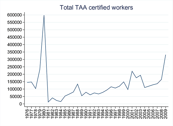
6.4 Standard Import Penetration Proxy
For a given location ![]() at a time
at a time ![]() , the "China syndrome"
measure used in Autor et al. (2013b) is an local import penetration measure:
, the "China syndrome"
measure used in Autor et al. (2013b) is an local import penetration measure:

Table 8 shows the typical order of magnitude of this import penetration proxy across states between 1988 and 2005. State-level time series of the ADH and the TAA measures are compared in Figure 11.
Table 8: Summary Statistics (1988-2005)
| Variable | p10 | p25 | p50 | p75 | p90 |
|---|---|---|---|---|---|
| Change in China import penetration in $000s per worker | 0.12 | 0.25 | 0.56 | 1.38 | 2.70 |
Figure 11: Time Series of Foreign Competition (1988-1997; 1999-2005)
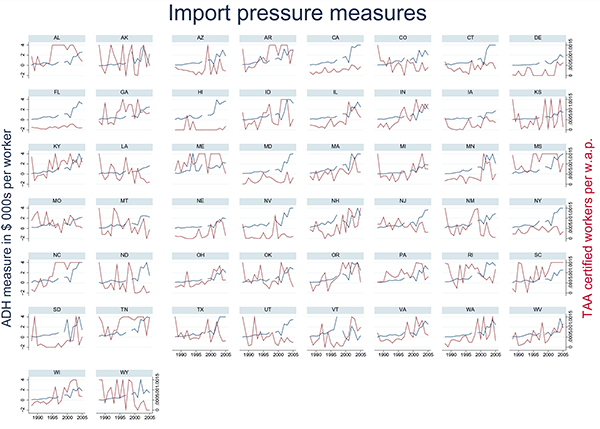
6.5 Other Labor Market Outcomes
See Table 9 for additional labor market outcomes.
Table 9: Other Labor Market Outcomes Panel Estimation Across the United States
| Labor market outcomes -> | Wages: e1 | Wages: e3 | Hours Worked: f1 | Hours Worked: f3 | Weeks Not Employed: g1 | Weeks Not Employed: g3 | Unemployed Workers: h1 | Unemployed Workers: h3 | Not in the Labor Force: i1 | Not in the Labor Force: i3 |
|---|---|---|---|---|---|---|---|---|---|---|
| Foreign Competition Variables: TAA Certified Workers | 0.910* (.498) |
1.809** (.750) |
-0.724** (.317) |
-1.011** (.386) |
5.021** (1.888) |
1.622 (2.663) |
1.010* (.587) |
1.584** (.775) |
2.227*** (.517) |
1.581* (.831) |
| Foreign Competition Variables: ADH Import Penetration | - - |
-0.0004 (.0007) |
- - |
-0.0006 (.0004) |
- - |
-0.0013 (.0026) |
- - |
-0.0007 (.0005) |
- - |
-0.0013* (.0007) |
| Additional Controls: TAA Denied Workers | 0.520 (.492) |
0.505 (0.628) |
-0.796 (.288) |
-1.113** (0.531) |
1.776 (1.678) |
-0.047 (2.506) |
-0.056 (.548) |
0.371 (.911) |
0.750 (.700) |
-0.608 (1.060) |
| Additional Controls: New Housing Starts | - - |
-0.397 (.372) |
- - |
0.697** (.314) |
- - |
-4.340*** (1.460) |
- - |
-0.652 (.507) |
- - |
-0.750 (.513) |
| Additional Controls: Unionization Rate | - - |
-0.047 (.032) |
- - |
-0.002 (.022) |
- - |
-0.202 (.135) |
- - |
-0.130*** (.037) |
- - |
-0.319*** (.054) |
| Standard Controls: Lagged outcome | Yes |
Yes |
Yes |
Yes |
Yes |
Yes |
Yes |
Yes |
Yes |
Yes |
| Standard Controls: Lagged foreign competition | Yes |
Yes |
Yes |
Yes |
Yes |
Yes |
Yes |
Yes |
Yes |
Yes |
| Standard Controls: Income (log) | Yes |
Yes |
Yes |
Yes |
Yes |
Yes |
Yes |
Yes |
Yes |
Yes |
| Standard Controls: U.S. population share | Yes |
Yes |
Yes |
Yes |
Yes |
Yes |
Yes |
Yes |
Yes |
Yes |
| Standard Controls: Year indicators | Yes |
Yes |
Yes |
Yes |
Yes |
Yes |
Yes |
Yes |
Yes |
Yes |
| Standard Controls: State indicators | Yes |
Yes |
Yes |
Yes |
Yes |
Yes |
Yes |
Yes |
Yes |
Yes |
| Standard Controls: Year x Region indicators | Yes |
Yes |
Yes |
Yes |
Yes |
Yes |
Yes |
Yes |
Yes |
Yes |
| R-sq. | 0.7397 |
0.8252 |
0.3474 |
0.1897 |
0.2135 |
0.2718 |
0.2293 |
0.3497 |
0.4525 |
0.5210 |
| N | 1350 |
750 |
1350 |
750 |
1350 |
750 |
1350 |
750 |
1350 |
750 |
Note: *, **, and *** denote significance at the 10, 5, and 1 percent level. Robust standard errors in parentheses are clustered on states. The estimation sample is a balanced panel of the 50 states that spans 27 years from 1983 and 2009. Union data is only available after 1989 in the March CPS. Import penetration can only be constructed between 1988 and 2005 with a gap in 1998 to a change from SIC to NAICS. All outcome variable are in log except the share of w.a.p. unemployed and the share of w.a.p. not in the labor force. Wages are usual hourly wages adjusted for top-coding and deflated using the national PCE deflator. Hours worked are total hours worked last year.
6.6 Additional Model Outcomes
Model predictions on medium-run earnings inequality and differences in employment rates are presented in 12.
Figure 12: Earnings and Employment Rates After Trade Reform
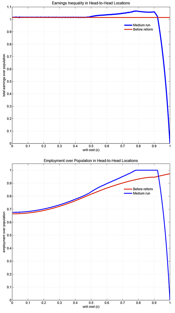
6.7 Productivity and Long-Run Outcomes
See Table 10 the long run effects of productivity.
Table 10: Long Run Labor Market Outcomes Across the United States
| Labor market outcomes -> | Not Employed in Five Years | Wages in Five Years | Population Share† in Five Years |
| Total Factor Productivity: Log TFP | 0.909*** (.233) |
23.05*** (4.250) |
.004* (.002) |
| Standard Controls: Lagged outcome | Yes |
Yes |
- |
| Standard Controls: U.S. population share | Yes |
Yes |
- |
| Standard Controls: Year indicators | Yes |
Yes |
- |
| Standard Controls: State indicators | Yes |
Yes |
- |
| R-sq. | 0.2002 |
0.5408 |
.0993 |
| N | 900 |
900 |
900 |
Note: *, **, and *** denote significance at the 10, 5, and 1 percent level. Robust standard errors in parentheses are clustered on states. The estimation sample is a balanced panel of the 50 states from 1983 and 2000. All outcome variable are in log except the share of w.a.p. unemployed and the share of w.a.p. not in the labor force. Waes are usual hourly wages adjusted for top-coding and deflated using the national PCE deflator. Hours worked are total hours worked last year.†: The population dynamics regression is a difference-in-difference estimation because the population thim series are not stationary.
6.8 Maps
Figures 13, 14, and 15 show maps of the TAA-based foreign competition measure.
Figure 13: Maps of Foreign Competition
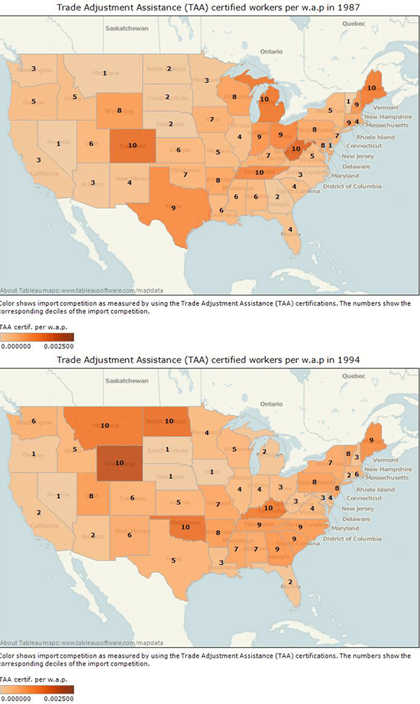
Figure 14: Maps of Foreign Competition
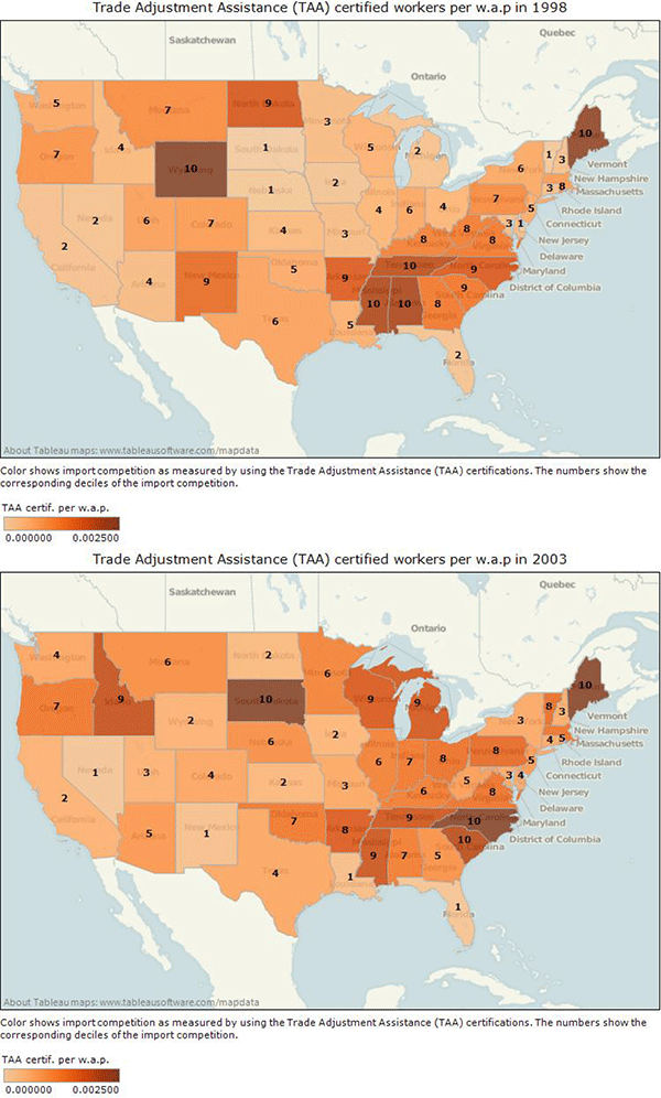
Figure 15: Maps of Foreign Competition
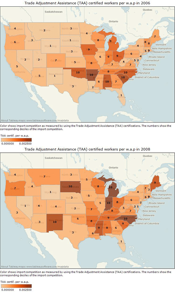
Footnotes
† First version: November 15, 2011. Return to text
** I thank Cristina Arellano, Tim Kehoe, and Fabrizio Perri for their continued, patient, and illuminating advice. I am deeply grateful to my discussants George Alessandria, Joel Rodrigue, and John Stevens for their excellent comments. I benefited from invaluable comments from David Autor, Wyatt Brooks, Rafael Dix-Carneiro, Alessandra Fogli, Jonathan Heathcote, Sewon Hur, Morris Kleiner, Brian Kovak, Logan Lewis, John Rogers, Gisela Rua, Edouard Schaal, Kjetil Storesletten, Olga Timoshenko, Kei-Mu Yi, and various seminar participants at the Cleveland Fed, Minneapolis Fed, Board, Minnesota, Clemson, Drexel, Northwestern, NUS, American, Vigo, Midwest Trade at MSU, SED in Seoul, RMEIT in Banff, and U.S. International Trade Commission. I thank Robert Tamura for the U.S. state productivity data. The data and programs used in the paper are available online. I gratefully acknowledge the University of Minnesota Doctoral Dissertation Fellowship for financial support. The views expressed herein are those of the author alone and not necessarily those of the Federal Reserve System. All errors and shortcomings are mine alone. Email: [email protected]. Return to text
1. Yotov (2007) and Uysal and Yotov (2011) previously used the underlying TAA petition data for industry-level and firm-level measures. Recently, Monarch et al. (2013) followed the same firm-level matching approach. A location-specific measure is used in this paper because of the salient geographic nature of labor markets. Margalit (2011) concurrently constructed a similar measure in the political science literature to study anti-incumbent voting behavior. Return to text
2. The nonemployment rate is the unemployment rate plus the non labor force participation rate. Return to text
3. In the standard Melitz (2003) model, a model-based TAA-measure of foreign competition is zero since firms do not face head-to-head direct competition: TAA investigators would be unable to find evidence of trade-induced foreign competition as a cause of layoffs. Return to text
4. This paper considers exogenous firm productivity differences for simplicity. See Glaeser and Maré (2001) and Combes et al. (2008) on agglomeration and worker selection across cities. Return to text
5. This indifference condition is reminiscent of Lewis (1954), Harris and Todaro (1970), spatial equilibrium models following Roback (1982), and directed search models such as Lucas and Prescott (1974) and Alvarez and Shimer (2011). Return to text
6. Kennan and Walker (2011), Artuç et al. (2010), Dix-Carneiro (2013) estimate substantial interim switching and mobility costs. These findings are consistent with the sluggish population adjustments found in this paper, Autor et al. (2013b), Menezes-Filho and Muendler (2011), and Topalova (2007). The assumption of limited ex post mobility made here follows Helpman and Itskhoki (2010). Return to text
7. Hasan et al. (2012) also investigate trade protection and unemployment across states in India. Return to text
8. A related literature investigates the decline of American manufacturing. Alder et al. (2012) and Yoon (2012) consider the role of unionization and biased technical change in the decline of the Rust Belt. See Holmes and Schmitz (2009) for a review of the literature on competition and productivity. Pierce and Schott (2012) also document that the elimination of trade policy uncertainty with China in 2000 contributed to the subsequent swift decline of American manufacturing. Return to text
9. Janiak (2006), Egger and Kreickemeier (2009), Dutt et al. (2009), Mitra and Ranjan (2010), and Felbermayr et al. (2010), and Helpman and Itskhoki (2010) among others subsequently introduced nonemployment in the baseline models of international trade. Return to text
10. See Notowidigdo (2011) and Moretti (2011) for studies on the effects of local shocks on wages and land prices using the spatial equilibrium framework of Roback (1982). Return to text
11. See appendix and online programs for details on the dataset. Return to text
12. All individual petitions are publicly available at http://www.doleta.govwww.doleta.gov. Return to text
13. See Decker and Corson (1994) and Magee (2001) and Park (2012) for papers using survey data on workers receiving TAA benefits to evaluate these programs. Return to text
14. A sample CDR form is available online at http://www.illenin.com/research/taa_cdr_article.pdfwww.illenin.com/research/taa_cdr_article.pdf. Return to text
15. See the appendix for maps and more summary tables and figures. Return to text
16. The weak correlation suggests that a decomposition of TAA-based job losses in industry, location, and firm effects using the ADH import penetration proxy at the commuting zone level is an important question. It is beyond the scope of this paper and therefore explored separately. Return to text
17. As found in the existing literature, the relationship with wages is not significant. Estimation results for wages and other labor market outcomes are reported in the appendix. Return to text
18. The sluggish population dynamics echo the findings of Autor et al. (2013b) and Topalova (2007). Klein et al. (2003) and Moser et al. (2010) also document similar effects of exchange rate fluctuations on job flows in the U.S. and in Germany respectively. Return to text
19. The Reagan administration drastically revamped the TAA certification process (see Rosen (2006)). That is the reason why the sample does not include the pre-Reagan reform era. Indeed, before 1983, the denied cases are associated with worsening labor markets and certified cases had an insignificant effect. In contrast, the findings reported here hold even if sample excludes the period after China's accession to the W.T.O. or the Great Recession. Return to text
20. As discussed in the previous subsection, the import penetration proxies ignore differences across firms and locations with similar industrial composition. Moreover, import penetration proxies suffer from an inherent degrees-of-freedom problem. This problem is solved with finer geographic granularity as discussed in Autor et al. (2013b). In contrast, the estimation with the TAA measure is done at the state level with region-time fixed effects. Return to text
21. This symmetry assumption is relaxed later. Return to text
22. This structure is similar to Alvarez and Shimer (2011) who consider a model with directed search across many islands and random matching within each island. Return to text
23. This form of head-to-head competition is similar to Bernard et al. (2003) with the distinction that there is no domestic head-to-head competitor here. See Caliendo et al. (2013) for a closed economy model with multiple locations and domestic competition. Return to text
24. The combination of both monopolistic competition and head-to-head
competition resembles the model of mass production plants and
boutique shops used by Holmes and Stevens (2010) in their
study of plant size distribution with an application to the trade
in wood furniture. Here, monopolistic firms are not necessarily smaller
non exporting firms. Also Freeman and Kleiner (2005) show in their
study of the "last American shoe manufacturers" that product differentiation
and industrial relations are additional channels of adjustment. Strategic
product differentiation will make
![]() endogenous. This
exogenous margin did not significantly alter the results from this
model when the differentiation costs are proportional to monopoly
profits.
Return to text
endogenous. This
exogenous margin did not significantly alter the results from this
model when the differentiation costs are proportional to monopoly
profits.
Return to text
25. The stark assumption on common productivity within a location is made to tractably highlight the role of variable markups. At the other extreme, if locations did not vary in productivity, this model would be unable to address the nonemployment effects of trade across locations. Return to text
26. Since the homogenous numeraire good is not traded, it is simply assigned a separate town. Return to text
27. For simplicity, one can think of Texas towns and Pennsylvania towns making cowboy hats and widgets respectively. Certainly, a location maps more realistically to a labor market in the geography-industry-occupation-skill space. Return to text
28. The Leontief matching function
![]() has no congestion externalities.
Return to text
has no congestion externalities.
Return to text
29. Due to variable markups, plant-level bargaining by destination market makes the bargaining outcome more tractable. Return to text
30. Nash-bargaining provides a simple and tractable baseline to highlight how nonemployment is determined. In this model, variable markups are key for the cross-sectional distribution of employment and wages. The alternative multilateral bargaining � la Stole and Zwiebel (1996) has been used in Felbermayr et al. (2010) and Helpman and Itskhoki (2010). Return to text
31. For the monopolist, casting the problem in terms of size (![]() )
or prices yield the same outcome.
Return to text
)
or prices yield the same outcome.
Return to text
32. See for example Felbermayr et al. (2010) and Helpman and Itskhoki (2010). Return to text
33. When
![]() , in particular in autarky, tariff-protected firms
price as monopolists even though they do not export.
Return to text
, in particular in autarky, tariff-protected firms
price as monopolists even though they do not export.
Return to text
34. Figure 5 illustrates the case when trade
barriers are low enough (
![]() ).
Return to text
).
Return to text
35. As trade barriers fall, some of the firms in this "dumping" region become monopolistic competitors both at home and abroad: trade barriers were hurting their competitive edge abroad. Other firms in this region now have to charge the competitor's marginal cost at home instead the monopolistic markup. Return to text
36. This model is quite tractable because of its block-recursive nature. Firms and households do not need to carry any cross-sectional distributions. While the model is simple in terms of firm and household optimizations, the general equilibrium has to be numerically computed because the non trivial double integration involved. Return to text
37. As in Helpman and Itskhoki (2010), the family interpretation is essential in the case of quasi-linear preferences but not when preferences are homothetic. Return to text
38. See the appendix for empirical evidence corroborating this relation between productivity and the nonemployment rate in the long run. Return to text
39. In the upper limit of autarky, the employment rate is constant since in all locations, all firms have a constant markup. See Table 3 for the other parameters used in the illustration. Return to text
40. The largest (proportional) firm expansions typically occur in the medium-sized locations that start exporting. This is reflected in the kink in Figure 7. Return to text
41.Melitz (2003) model and similar models with no direct competition, a TAA-measure of import competition would always be zero because the firms do not shut down because of direct foreign competition: TAA investigators would be unable to find evidence for trade-induced foreign competition as a cause of the layoffs. Return to text
42. The model results are reported along the continuum of locations. These results can certainly be aggregated by statistical units called "states" where each state is a selection of locations with correlated productivity. The current exposition is simpler and easier to connect to the mechanism in the model. Return to text
43. In fact, the calibration target is rather conservative since ![]() is chosen to match the nationwide average fraction of trade-displaced
workers certified by the TAA.
Return to text
is chosen to match the nationwide average fraction of trade-displaced
workers certified by the TAA.
Return to text
44. Welfare gains would be different in the absence of full insurance across locations. A richer and more complex model with incomplete markets such as Krusell et al. (2010) would be needed. The implications of limited insurance during trade reforms go beyond the scope of this paper. Return to text
45. Income is not included since it is strongly correlated with productivity. Return to text
46. The large elasticity of nonemployment rate to trade-displacements can only be rationalized by this model when petitions mainly come from the hardest hit locations as shown in Figure 8. Return to text
47. In contrast with specifications (b4) and (c4), the effects of trade-induced displaced are no longer significant once productivity is included. Return to text
48. Foreign competitors are randomly reassigned a new productivity according
to the new distribution. Trade barriers are set to ![]() before
and after the change. See Table 3 for the other
parameters.
Return to text
before
and after the change. See Table 3 for the other
parameters.
Return to text
49. Individual petitions are publicly available at http://www.doleta.gov/tradeact/taa/taa_search_form.cfmwww.doleta.gov/tradeact/taa/taa_search_form.cfm Return to text
This version is optimized for use by screen readers. Descriptions for all mathematical expressions are provided in LaTex format. A printable pdf version is available. Return to text