FEDS Notes
May 21, 2019
Tips from TIPS: Update and Discussions
Don Kim, Cait Walsh (Columbia Business School), and Min Wei1
- Introduction
The spread between the yield on a nominal Treasury security and that on a Treasury inflation protected security (TIPS) of comparable maturities—usually called the "breakeven inflation rate" or "inflation compensation"—has been often used as a real-time proxy for market participants' inflation expectations. However, policymakers and market participants are also cognizant that this spread is an imperfect measure, as it contains other components that can drive a wedge between inflation compensation and market participants' true inflation expectations.
In a recently published paper (D'Amico, Kim, and Wei (DKW), 2018), D'Amico and two of us use a no-arbitrage term structure model to decompose TIPS inflation compensation into three components—inflation expectation, inflation risk premium, and TIPS liquidity premium—over the 1990-2013 period. The model is also used to decompose nominal yields or forward rates into four components—expected real short rate, expected inflation, inflation risk premium, and real term premium.
In this Note, we update and extend the estimation to a longer period from 1983 to the present. The additional sample includes the period over which longer-term inflation expectations moved down significantly following the Volcker disinflation, which may help in pinning down the dynamics of the persistent components of inflation and inflation expectations.2 After reviewing some basic aspects of the model, we discuss correlations of longer-horizon inflation compensation with risk sentiment proxies and with oil prices, and compare our model implied estimates of longer-run inflation expectations and equilibrium real rate with other estimates in the literature.
- A brief review of the DKW model
The DKW model is a no-arbitrage term structure model, in which nominal yields, real yields, and inflation expectations are all assumed to be affine (i.e. linear) functions of latent factors that follow normal distributions. The model is specified in a "maximally flexible" way, i.e., the parameterization of the model is of the most general form that can be econometrically identified for the given assumptions. The model allows TIPS yields to deviate from "true" real yields. This differential, which we call "TIPS liquidity premium" as it primarily reflects the lower liquidity of TIPS relative to nominal Treasury securities, is modeled as an affine function of the latent factors that are common to nominal and real yields and an additional latent factor that is independent of the common factors.
By standard economic theory, nominal and real yields can be decomposed as:
nominal yield = real yield + expected inflation + inflation risk premium; (1)
real yield = expected average future real short rate + real term premium, (2)
where the inflation risk premium and the real term premium are extra compensations bond investors demand for bearing inflation risks and real interest rate risks, respectively. Nominal and real forward rates can be decomposed in the same way.
In the model, TIPS yields typically exceed "true" real yields (or real yields that are consistent with nominal yields) due to the TIPS liquidity premium:3
TIPS yield = real yield + TIPS liquidity premium. (3)
As a result, TIPS inflation compensation (IC)—defined as the nominal yield minus the TIPS yield—can be decomposed into three components,
TIPS IC = expected inflation + inflation risk premium – TIPS liquidity premium. (4)
TIPS IC can deviate from expected inflation for two reasons: a non-zero inflation risk premium or a non-zero TIPS liquidity premium. The first term, inflation risk premium, is the extra compensation nominal bond investors demand for bearing inflation risks, and its value depends on the covariance between inflation and real economic activity. This premium is believed to have been positive and sizeable in the 1970s and 1980s, when investors were more worried about stagflation scenarios with higher inflation accompanied by lower growth, but appears to have declined in recent decades to lower or even negative levels, as investors have become more concerned about outcomes where lower inflation is associated with lower growth.4
By contrast, TIPS liquidity premium is not connected to inflation risk but rather reflects factors that drive a wedge between TIPS yields and true real yields. This premium was high when TIPS was first launched, as it took some time for TIPS to gain popularity among investors, and again surged during the 2008-2009 Financial Crisis, as investors fled from less liquid or more risky instruments and sought the safety and liquidity of nominal Treasury securities. Apart from lower liquidity of TIPS relative to nominal Treasuries, this premium may also reflect supply-demand imbalance of TIPS versus nominal securities and a greater concentration of buy-and-hold investors in TIPS market compared with the nominal Treasury market.
Following DKW, we estimate the model with weekly data on nominal yields, TIPS yields and monthly data on seasonally-adjusted CPI, supplemented by survey forecasts of inflation and 3-month T-bill yield to address small sample problems associated with persistent time series such as interest rates.5,6 To extend the estimation, we use nominal Treasury yields and survey forecasts from January 1983 to May 2018.7
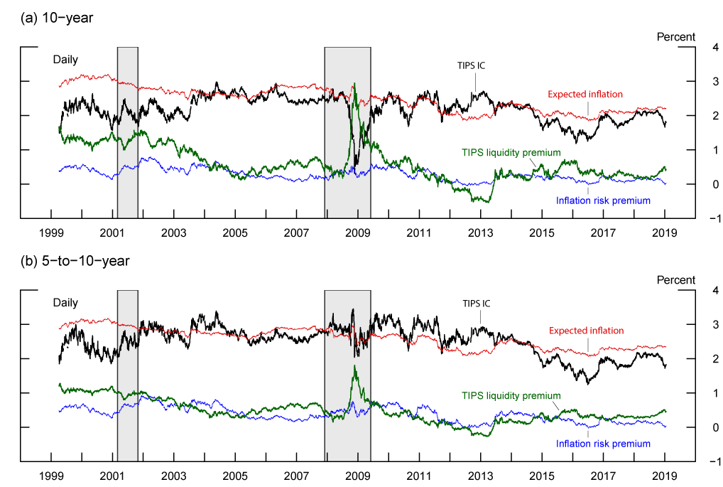
Source: D'Amico, Kim, and Wei (2018), updated by authors.
The upper and lower panels of Figure 1 show decompositions of 10-year and 5-to-10-year TIPS IC, respectively, into the three components according to Equation (4), based on the updated DKW model. TIPS inflation compensations move around a fair bit, even at the 5-to-10-year horizon where market participants and policymakers often look for signals regarding longer-horizon inflation expectations, and are substantially more volatile than the model-implied inflation expectations. The variations in model-implied inflation risk premium and TIPS liquidity premium follow the patterns outlined in the previous paragraphs.
- Relationship of longer-horizon IC with sentiment proxies and oil prices
Longer-horizon TIPS IC not only moves around quite a bit, but also tends to co-move with variables that proxy for changing market sentiment. For example, Figure 2 shows a visible negative correlation between the 5-to-10-year IC and the high-yield (HY) corporate bond spread (upper panel) or the VIX (middle panel).8 Over the period since 2014, longer-horizon TIPS IC also appears to comove with oil prices, as both IC and oil prices declined notably in 2014H2 and in late 2018.9
Figure 2: Comovement between 5-to-10-year TIPS inflation compensation and market sentiment proxies or oil prices
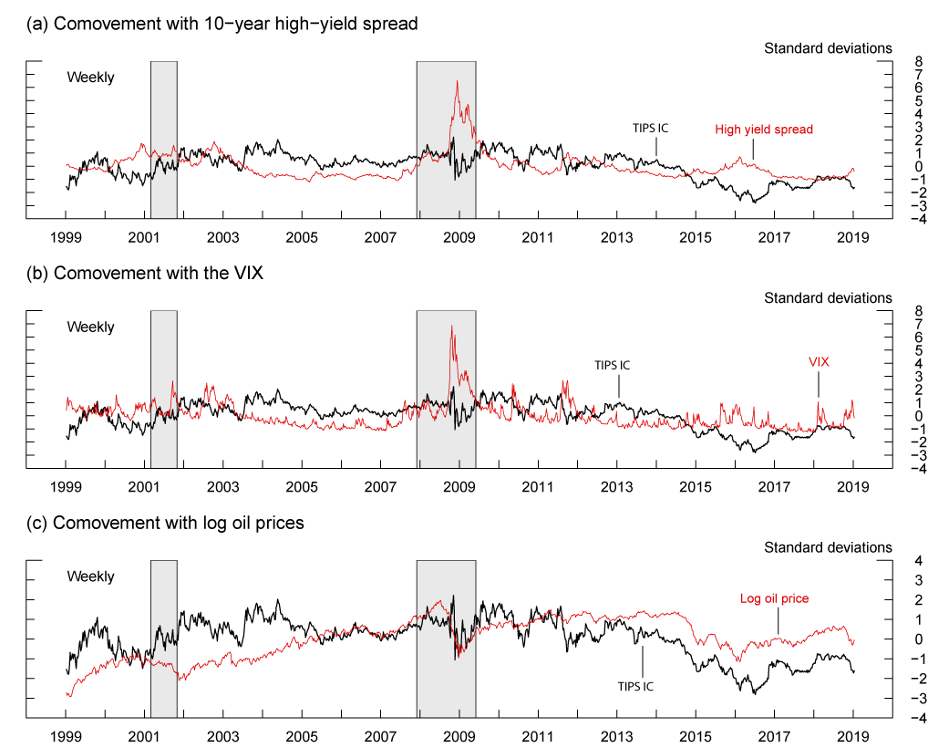
Note: All figures have been standardized, i.e., they have been subtracted by the mean and then divided by the standard deviation. The inflation compensation series in (c) is identical to the series in (a) and (b), but has been plotted with a different vertical scale.
Source: Bloomberg; Board staff estimates.
These visual impressions are confirmed by Panel A of Table 1, which shows pairwise correlations between weekly changes in TIPS IC and its model-implied components, on the one hand, and the two sentiment proxies and oil prices, on the other, for the full sample since 1999. Changes in IC covary negatively with those in the HY spread and in VIX, and positively with those in oil prices. The magnitudes of correlations are higher in the post-crisis period (Panel C) and lower in the pre-crisis period (Panel E). The co-movements of IC with HY spread and VIX appear more elevated when there are notable shifts in risk sentiments. As can be seen from Panels B and D, the correlations of VIX and IC in weeks when VIX moves by more than one standard deviation is substantially larger in magnitude than the corresponding unconditional correlations both over the full sample and since the crisis.10
Table 1: Correlation of 5-to-10-year TIPS IC with sentiment indicators and oil prices
| Unconditional correlation | Conditional correlation | |||||||
|---|---|---|---|---|---|---|---|---|
| IC | IE | IRP | LP | IC | IE | IRP | LP | |
| Panel A: full sample (1999-present) | Panel B: full sample (1999-present) | |||||||
| HY spread | -0.33 | -0.27 | -0.37 | 0.27 | -0.4 | -0.22 | -0.28 | 0.48 |
| VIX | -0.22 | -0.12 | -0.21 | 0.16 | -0.35 | -0.17 | -0.33 | 0.22 |
| oil prices | 0.18 | 0.16 | 0.14 | -0.19 | 0.36 | 0.3 | 0.29 | -0.11 |
| Panel C: post-crisis (July 2009-present) | Panel D: post-crisis (July 2009-present) | |||||||
| HY spread | -0.53 | -0.59 | -0.67 | 0.12 | -0.65 | -0.74 | -0.81 | 0.28 |
| VIX | -0.35 | -0.31 | -0.38 | 0.17 | -0.52 | -0.55 | -0.64 | 0.24 |
| oil prices | 0.25 | 0.19 | 0.24 | -0.32 | 0.43 | 0.4 | 0.47 | -0.41 |
| Panel E: pre-crisis (1999-July 2008) | Panel F: pre-crisis (1999-July 2008) | |||||||
| HY spread | -0.31 | -0.3 | -0.49 | -0.01 | -0.31 | -0.25 | -0.43 | 0.06 |
| VIX | -0.01 | -0.03 | -0.12 | -0.06 | -0.02 | -0.01 | -0.16 | -0.07 |
| oil prices | 0.06 | 0 | -0.08 | -0.27 | 0.14 | 0.03 | -0.02 | -0.2 |
Note: Correlation of weekly changes. Oil-price correlations are computed with changes in log oil price. "Conditional correlation" refers to the correlation when the magnitude of weekly change in VIX is greater than one standard deviation of the respective sample.
Source: Bloomberg, Board staff estimates.
The correlation between risk sentiments indicators and the longer-horizon IC could arise from two channels. First, deteriorating risk sentiment is generally accompanied by, if not triggered by, perception of increased downside risks to growth. As mentioned earlier, in recent decades market participants appear to associate lower inflation with states of the world with lower real economic growth. As a result, perception of increased downside risk would likely push down both the inflation risk premium component and the expected inflation component of TIPS IC. Second, episodes of deteriorating risk sentiments are typically associated with strong safe haven flows into nominal Treasury securities. The increased demand for nominal Treasury securities would push up nominal Treasury prices relative to TIPS, resulting in higher TIPS liquidity premium. The patterns in Table 1 are consistent with both of these effects: Model-implied inflation expectation and inflation risk premium are negatively correlated with, while the TIPS liquidity premium is positively correlated with, the HY spread and the VIX.
The positive correlation between longer-horizon IC and oil prices is more puzzling. Food and energy prices are part of the (total) CPI to which TIPS are indexed, so it is natural to expect some correlation between near-term IC and oil prices, but it is less clear what mechanism underlies the comovement for longer-horizon IC. In 2014H2 and late 2018 when both oil prices and IC declined notably, a substantial fraction of these oil-price declines seemed to be driven by an oversupply of oil.11 But concerns about weaker global demand and deteriorated risk sentiment may also have contributed to oil-price declines. If we compute the correlation of oil prices and longer-horizon IC using only observations when VIX moved more than one standard deviation (i.e., weeks with substantial changes in risk sentiment), the magnitude of oil price and IC correlation almost doubles, as can be seen in Table 1 (e.g., from 0.18 to 0.36 in the 1999-present sample), suggesting that common factors, such as risk sentiment, may have contributed to the variations in both series.
- Longer-horizon inflation expectations (π*)
Longer-horizon inflation expectations are of considerable interest to investors, policymakers and researchers alike. As discussed above, it is natural to view that bond prices, being set by forward-looking market participants, embed this information, but some modeling is necessary to separate out other components of TIPS IC. The black line in Figure 3 presents the estimate of the 5-to-10-year inflation expectation going back to 1983 based on the updated DKW (2018) model.
Other researchers in the Federal Reserve System, including Abrahams, Adrian, Crump, Moench, and Yu (henceforth AACMY, 2016), Ajello, Benzoni, and Chyruk (henceforth ABC, 2012), Christensen, Lopez, and Rudebusch (henceforth CLR, 2010), and Haubrich, Pennacchi, and Ritchken (henceforth HPR, 2012), also developed term structure models that can be used to generate real-time measures of inflation expectations. Apart from nominal Treasury yields and inflation, the HPR model uses inflation swaps instead of TIPS yields. The AACMY and the CLR models use TIPS yields, where AACMY model the TIPS liquidity premium as a function of observable liquidity metrics while CLR ignore the lower liquidity of TIPS and exclude the earlier sample of TIPS. The ABC model does not use either inflation swap or TIPS in the estimation.12,13,14,15
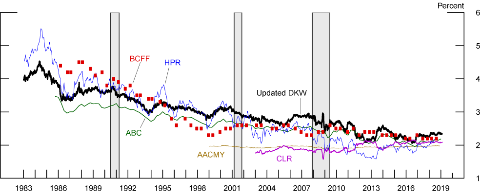
Note: BCFF is the (approximately) 5-to-10-year CPI inflation forecast from the semi-annual Blue Chip Financial Forecasts survey. The ABC estimate is reported at a quarterly frequency. The HPR estimate is reported at a monthly frequency. The AACMY, CLR, and Updated DKW estimates are reported at a daily frequency.
Source: Abrahams, Adrian, Crump, Moench, and Yu (2016); Ajello, Benzoni, and Chyruk (2012); Christensen, Lopez, and Rudebusch (2018); Haubrich, Pennacchi, and Ritchken (2012); Blue Chip Financial Forecasts; D'Amico, Kim, and Wei (2018) updated by authors.
As can be seen from Figure 3, the estimates of longer horizon inflation expectations can vary significantly across models. The AACMY measure was practically immobile during the entire period for which the data were available. The CLR measure is also very stable up to 2011. By contrast, our measure and the ABC and HPR measures show higher variabilities as well as a notable downward trend since early 1980s, consistent with Blue Chip Financial Forecasts (BCFF) survey forecast of inflation 5 to 10 years ahead. Over the past decade the three measures show very similar variations, although the updated DKW and the ABC measure lie somewhat above the HPR measure. The range of these estimates has narrowed over time and currently varies from 2% (AACMY) to 2.4% (updated DKW) for CPI inflation, or roughly 1.7% to 2.1% for PCE inflation after taking into account the level difference between the two inflation measures.
One may view the extreme stability of the AACMY measure as evidence that the market's longer-horizon inflation expectations are very well anchored. However, it seems more likely to us that the apparent stability reflects the small sample problems noted in footnote [6] that standard implementations of term structure models frequently encounter; as a result, the persistence of (expected) inflation in that model were likely underestimated such that inflation expectations revert to its long-run mean in less than 5 years, leaving little variations beyond that horizon.
- Longer-run equilibrium real rate (rLR)
Another interesting object the model can shed light on is the expected real short rate 5-to-10-years ahead, which can be viewed as a measure of the equilibrium level of the real federal funds rate in the longer run (rLR), defined as the rate consistent with the economy operating at its potential once the transitory effects of economic shocks have abated. Figure 4 compares our rLR estimates with those from the other term structure models discussed above (AACMY, ABC, CLR, and HPR) and a real term structure model developed by Christensen and Rudebusch (CR) (2017) and estimated using TIPS yields only. The range of rLR estimates across models is quite wide and currently much wider than that seen in Figure 3 for inflation expectations. The AACMY measure hovered near zero for the entire period since the late 1990s, spending nearly half of the time in the negative territory, and lay below all other measures up to the crisis. The CLR measure, on the other hand, provided the upper end of the range over most of its sample since 2003 and is currently at 1.4%. Our measure is closest to the CR measure in terms of level and variabilities.
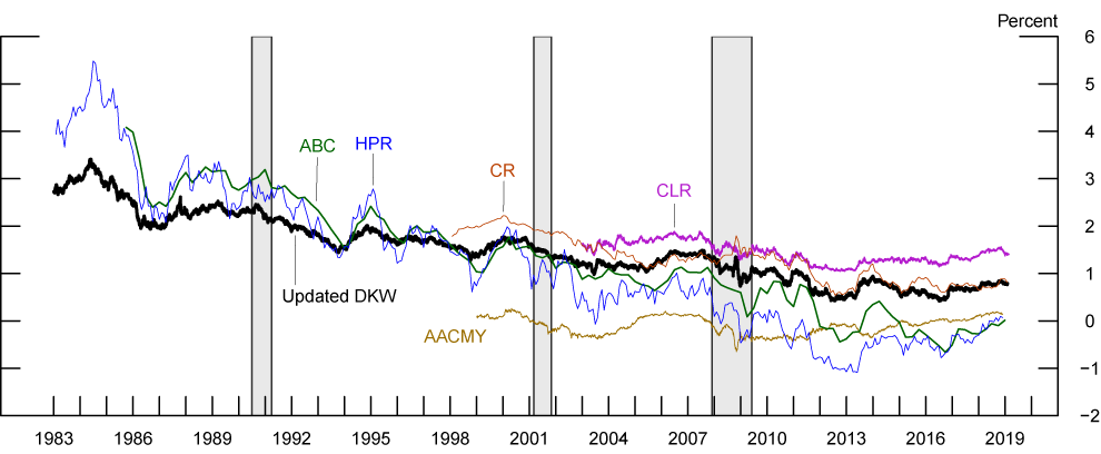
Note: The AACMY, CLR, and Updated DKW estimates are reported at a daily frequency. The CR and HPR models are reported at a monthly frequency. The ABC model is reported at a quarterly frequency.
Source: Abrahams, Adrian, Crump, Moench, and Yu (2016); Ajello, Benzoni, and Chyruk (2012); Christensen, Lopez, and Rudebusch (2010); Christensen and Rudebusch (2017); Haubrich, Pennacchi, and Ritchken (2012); D'Amico, Kim, and Wei (2018) updated by authors.
Estimates of rLR can also be obtained from macro models, where time-series methods can be used to infer rLR from the co-movement of macroeconomic series such as inflation, interest rates, and output. Figure 5 plots several such measures constructed by researchers at the Federal Reserve System—Del Negro, Giannone, Gianonni, and Tambalotti (henceforth DNGGT, 2017), Holston, Laubach, and Williams (henceforth HLW, 2017), Johannsen and Mertens (henceforth JM, 2016), Kiley (2015), Lewis and Vazquez-Grande (henceforth LVG, 2017), and Lubik and Matthes (henceforth LM, 2015). With the exception of JM, all models show a pronounced decline in rLR around the 2008-2009 financial crisis.
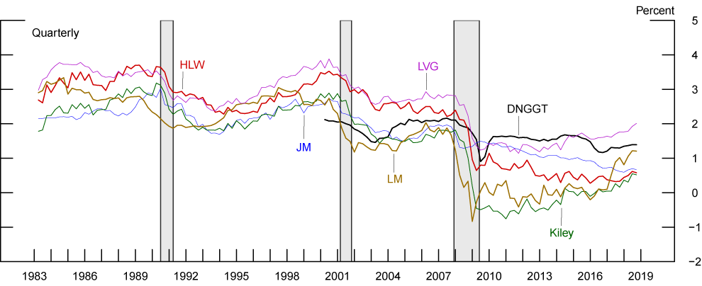
Note: All model estimates are in quarterly frequency and are filtered estimates (as opposed to smoothed estimates).
Source: Del Negro et al. (2017); Holston, Laubach, and Williams (2017); Johannsen and Mertens (2016); Kiley (2015); Lewis and Vazquez-Grande (2017); Lubik and Matthes (2015).
Figure 6 shows our measure and a survey-based measure, against the backdrop of the range of those macro model-based estimates. Similar to the JM measure in Figure 5, our model indicates a more gradual downward drift in rLR over the past couple of decades. Our measure has stayed within the range of macro model estimates since the crisis, but lies at or below the bottom of the range for most of the pre-crisis years. Our measure is close to the survey-implied measure in recent years but exhibits somewhat less variability over the longer span of time since mid-1980s.16
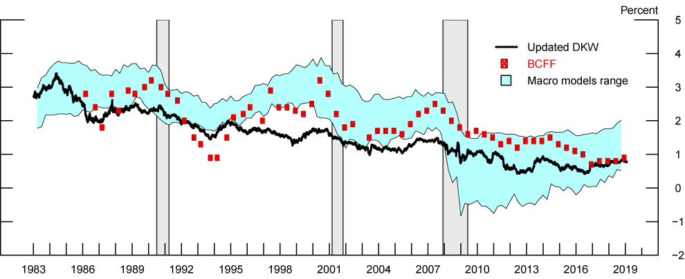
Note: BCFF is the neutral real interest rate implied by the Blue Chip Financial Forecasts Survey. It is calculated as the difference between the 5-to-10-year expected federal funds rate minus the 5-to-10-year expected CPI inflation. The blue shaded region shows the range of macro model estimates in Figure 5.
Source: D'Amico, Kim, and Wei (2018) updated by authors; Blue Chip Financial Forecasts; Del Negro et al. (2017); Holston, Laubach, and Williams (2017); Johannsen and Mertens (2016); Kiley (2015); Lewis and Vazquez-Grande (2017); Lubik and Matthes (2015).
All measures in Figures 5 and 6 share the feature that rLR is currently lower than its average values in 1990s and before the financial crisis, implying that in the current tightening cycle policymakers might not have to raise rates to the same level as they had done in the past tightening episodes. That said, the range of rLR estimates is currently pretty wide, ranging between 0.5 and 2 percent, which underscores the importance of cautiously evaluating incoming data to assess the stance of monetary policy. In addition, estimates of rLR appear to vary substantially depending on modeling and implementation choices. While certain choices may arguably be justifiable than others, it is important to keep in mind that expectations and risk attitudes, which ultimately determine market prices of nominal and TIPS securities, are quite complex, and models are only approximate representations of the rich behaviors of the yield curve and the economy. Caution is therefore always warranted in interpreting rLR estimates or any other outputs from models.
- Data release
Beginning with the publication of this Note, we will provide monthly updates of model decompositions of the 5-year, 10-year, and 5-to-10-year nominal Treasury yields and inflation compensation up to the last business day of the previous month. In general, we will endeavor to have the updated series posted sometime after 10:00 a.m. on the fourth business day of each month. Because this is a staff research product and not an official statistical release, it is subject to delay, revision, or methodological changes without advance notice.17
The latest estimates will be posted as a comma-separated values (CSV) file at the URL https://www.federalreserve.gov/econres/notes/feds-notes/DKW-updates.csv. As of this publication, daily data are available for the period from January 3, 1983 to January 31, 2026.
References
Abrahams, M., T. Adrian, R. K. Crump, E. Moench, and R. Yu (2016), "Decomposing real and nominal yield curves," Journal of Monetary Economics, 84, pp. 182-200.
Ajello, A., L. Benzoni, O. Chyruk (2012), "Core and 'Crust': Consumer Prices and the Term Structure of Interest Rates," working paper. (Forthcoming in Review of Financial Studies.)
Campbell J. Y., A. Sunderam, and L. M. Viceira (2017), "Inflation Bets or Deflation Hedges? The Changing Risks of Nominal Bonds," Critical Finance Review, 6, pp. 263-301.
Christensen, J. H.E., J. A. Lopez, and G. D. Rudebusch (2010), "Inflation Expectations and Risk Premiums in an Arbitrage-Free Model of Nominal and Real Bond Yields," Journal of Money, Credit and Banking, 42(S1), pp. 143-178.
Christensen, J. H.E. and Rudebusch, Glenn D. (2017), "A New Normal for Interest Rates? Evidence from Inflation-Indexed Debt," Working Paper Series 2017-7, Federal Reserve Bank of San Francisco. (Forthcoming in Review of Economics and Statistics.)
D'Amico, S., D. H. Kim, and M. Wei (2018), "Tips from TIPS: The Informational Content of Treasury Inflation-Protected Security Prices," Journal of Financial and Quantitative Analysis, 53(1), 395-436.
Del Negro, M., D. Giannone, M. P. Giannoni, and A. Tambalotti (2017). "Safety, Liquidity, and the Natural Rate of Interest," Brookings Papers on Economic Activity, Spring, pp. 235-316.
Forbes, K. J. and R. Rigobon (2002), "No Contagion, Only Interdependence: Measuring Stock Market Comovements," Journal of Finance, 57, pp. 2223-2261.
Gospodinov, N. (2017), "Asset Co-movements: Features and Challenges," Working Paper Series 2017-11, Federal Reserve Bank of Atlanta.
Haubrich, J., G. Pennacchi, and P. Ritchken (2012), "Inflation Expectations, Real Rates, and Risk Premia: Evidence from Inflation Swaps," Review of Financial Studies, 25 (5), pp. 1588–1629.
Holston, K., T. Laubach, and J. C. Williams (2017). "Measuring the Natural Rate of Interest: International Trends and Determinants," Journal of International Economics, 108, pp. S59-75.
Johannsen, B. K. and E. Mertens (2016), "A Time Series Model of Interest Rates with the Effective Lower Bound," Finance and Economics Discussion Series 2016-033. Board of Governors of the Federal Reserve System.
Kiley, M. T. (2015). "What Can the Data Tell Us about the Equilibrium Real Interest Rate?" Finance and Economics Discussion Series 2015-077. Board of Governors of the Federal Reserve System.
Kim, D. H. and A. Orphanides (2012), "Term Structure Estimation with Survey Data on Interest Rate Forecasts," Journal of Financial and Quantitative Analysis, 47(1), pp. 241-272.
Lewis, Kurt F., and Francisco Vazquez-Grande (2017), "Measuring the Natural Rate of Interest: A Note on Transitory Shocks," Finance and Economics Discussion Series 2017-059r1. Board of Governors of the Federal Reserve System. (Forthcoming in Journal of Applied Econometrics.)
Loretan, M. and W. B. English (2000). "Evaluating "Correlation Breakdowns" During Periods of Market Volatility," International Finance Discussion Papers 658. Board of Governors of the Federal Reserve System.
Lubik, T. A. and C. Matthes (2015). "Time-Varying Parameter Vector Autoregressions: Specification, Estimation, and an Application," Economic Quarterly, 101 (Q4), pp. 323-52.
Stillwagon, J. R. (2018). "TIPS and the VIX: Spillovers from Financial Panic to Breakeven Inflation in an Automated, Nonlinear Modeling Framework," Oxford Bulletin of Economics and Statistics, 80, pp 218-235.
1. Kim and Wei are with the Board of Governors of the Federal Reserve System, and Walsh is with Columbia Business School. We thank Richard Crump, Ben Johannsen, Thomas Laubach, Kurt Lewis, and Glenn Rudebusch for helpful comments, and Paul Cordova and Gerardo Sanz-Maldonado for research assistance. Return to text
2. We start our data from 1983, as the early 1980s ("Volcker experiment" period) had much higher yield volatilities and possibly other qualitative differences relative to later times. Return to text
3. DKW (2018) shows that models estimated under the assumption of zero TIPS liquidity premium not only do poorly in fitting TIPS yields but also have unreasonable implications for key variables such as inflation expectations and inflation risk premia. Return to text
4. Such a mechanism is discussed in Campbell, Sunderam, and Viceira (2017). Return to text
5. The data inputs include: 3- and 6-month, 1-, 2-, 4-, 7-, and 10-year nominal Treasury yields (weekly); 5-, 7- and 10-year TIPS yields (weekly); 6- and 12-month-ahead BCFF forecasts of the 3-month T-bill rate (monthly); BCFF long-range (5-10 years ahead) forecasts of the 3-month T-bill rate (semiannual); median SPF forecasts of average inflation over the following year and over the next 10 years (quarterly). Return to text
6. Standard estimation of models with persistent time series data often leads to downward bias in estimates of persistence coefficients and to imprecision in parameter estimates. For more discussion on these small sample problems, see Kim and Orphanides (2012). Return to text
7. We treat the earlier period without TIPS data (1983-1998) as missing observations. From January 1983 through November 1989, we replace 3- and 6-month T-bill rates with zero-coupon fitted nominal yields of the same horizons in order to avoid problems arising from the market's flight to bills around 1987, which caused considerable deviation of bill yields from the coupon curve. We linearly splice fitted and actual T-bill yields over the course of December 1989 to facilitate a smoother transition. Return to text
8. Stillwagon (2018) shows that spot measures of TIPS IC, such as the 5-year and 10-year ICs, comove even more with the VIX than the 5-to-10-year TIPC IC discussed here. Return to text
9. Gospodinov (2017) also discusses the correlation between the 5-to-10-year IC and oil prices, focusing on the 2014-16 period. Return to text
10. Part of this may be due to a statistical artifact. As discussed by Loretan and English (2000) and Forbes and Rigobon (2002), the correlation of two random variables A and B, conditional on A being larger (in magnitude) than usual, is larger than the unconditional correlation of A and B. Return to text
11. On many of the days in which oil prices fell notably, there were news related to oil supply. Return to text
12. The HPR model assumes that nominal and real yields are driven by three factors representing the short-term real interest rate, expected inflation, and long-run inflation, respectively, as well as four volatility factors that follow GARCH processes. The model is estimated using nominal Treasury yields, inflation swaps and survey inflation forecasts. Return to text
13. The AACMY model assumes that nominal Treasury and TIPS yields are all driven by six observable factors: the first three principal components of nominal Treasury yields, a TIPS liquidity factor, and the first two principal components of the part of TIPS yields not explained by the nominal or liquidity factors. The TIPS liquidity factor is constructed by averaging the average absolute TIPS yield curve fitting error and the relative Primary Dealer transaction volumes in Treasuries versus TIPS. The model is estimated using nominal Treasury and TIPS prices and monthly CPI inflation since 1999. Return to text
14. The CLR model assumes that nominal and TIPS yields are driven by two separate level factors but share the same slope and curvature factors. Restrictions are imposed on the dynamics of the state variables such that both nominal and real yields follow the Nelson-Siegel functional form. The model is estimated using nominal yields from January 6, 1995 to March 28, 2008 and TIPS yields from January 3, 2003 to March 28, 2008. Return to text
15. The ABC model is a no-arbitrage term structure model of nominal yields and inflation. The model has both latent and observable factors, with multiple inflation series, more specifically the core, food, and energy prices, serving as the observable factors. Return to text
16. As noted in footnote [5], the model is estimated using data on 10-year ahead SPF inflation forecast but not the BCFF long-range inflation forecast. Return to text
17. On the rare occasion when source data are unavailable or delayed, the updated estimates will be posted as soon as feasible. Additionally, in situations when the scheduled release falls during the FOMC communications blackout period (PDF), the updated series will be posted after the blackout period has ended. Return to text
Kim, Don, Cait Walsh, and Min Wei (2019). "Tips from TIPS: Update and Discussions," FEDS Notes. Washington: Board of Governors of the Federal Reserve System, May 21, 2019, https://doi.org/10.17016/2380-7172.2355.
Disclaimer: FEDS Notes are articles in which Board staff offer their own views and present analysis on a range of topics in economics and finance. These articles are shorter and less technically oriented than FEDS Working Papers and IFDP papers.