IFDP Notes
January 12, 2018
Differences in Stock Returns of U.S. Firms with High and Low Tradability
Since the beginning of 2017, the trade-weighted value of the dollar has depreciated by over 8 percent, weakening broadly against both advanced and emerging market economies' currencies. At the same time, economic activity has been rising moderately. What role do these factors play in equity prices, where over the same period, the U.S. S&P 500 index is up over 20 percent?
Intuitively speaking, a weaker currency tends to benefit exports-producing firms as the cost of their goods that are sold abroad is relatively cheaper. Indeed, since the beginning of 2017, stocks of U.S. firms with high international sales have risen notably more than U.S. firms with low international sales.2 Given this backdrop, a policy-relevant question is (a) understanding the broader effects of economic fundamentals and exchange rate movements on the equity performance of U.S. firms and (b) how these effects vary with how export-oriented a firm is.
In a forthcoming paper at the Journal of Financial Economics, I examine the effect of a U.S. firm's tradability--defined as the proportion of output that is exported abroad--on its stock returns over business cycles from 1947-2015.3 I consider the differential impacts of economic growth and exchange rate movements on the stock returns of U.S. firms ranked by tradability. The two main findings in the paper are: (1) Firms with high tradability have asset returns that significantly co-move more with economic growth than firms with low tradability; (2) The difference in stock returns between firms with the highest tradability and firms with the lowest tradability can predict changes in the real dollar exchange rate.
In this note, I summarize the methodology and findings of my research paper and draw out the policy implications. The effects of GDP growth appear to matter more but the link between exchange rates and stock returns is also economically and statistically significant. The policy implications are that the spread in returns between U.S. firms with high and low tradability could provide a hedge against recessions. At the same time, stock returns are also informative about future exchange rate movements.
Measuring tradability
Tradability is defined as the extent to which a firm sells its products abroad, specifically, the share of its output that is exported. Using the 2002 Bureau of Economic Analysis's National Income and Product Account (BEA NIPA) Input-Output Tables, described in Stewart, Stone, and Streitwieser (2007), I first compute tradability ratios by industry (the value of exports over the total industry output) for over 400 industries in the U.S.
Table 1: Top and Bottom Ten Industries by Tradability Ratio (2002)
| Industry | Trad Ratio | Description |
|---|---|---|
| 333314 | 0.88 | Optical instrument and lens mfg |
| 114100 | 0.74 | Fishing |
| 333130 | 0.64 | Mining and oil and gas field machinery mfg |
| 336413 | 0.57 | Other aircraft parts and auxiliary equipment mfg |
| 33399A | 0.55 | Other general purpose machinery mfg |
| 336412 | 0.54 | Aircraft engine and engine parts mfg |
| 333994 | 0.53 | Industrial process furnace and oven mfg |
| 334513 | 0.52 | Industrial process variable instruments mfg |
| 316100 | 0.51 | Leather and hide tanning and finishing |
| 334411 | 0.5 | Electron tube mfg |
Bottom Ten:
| Industry | Trad Ratio | Description |
|---|---|---|
| 213111 | 0.00004 | Drilling oil and gas wells |
| 811192 | 0.000019 | Car washes |
| 624200 | 0.000017 | Community food housing and other relief services |
| 525000 | 0.000014 | Funds, trusts, and other financial vehicles |
| 812900 | 0.000012 | Other personal services |
| 812300 | 0.000008 | Dry-cleaning and laundry services |
| 812200 | 0.000004 | Death care services |
| 624400 | 0.000002 | Child day care services |
| 812100 | 0.000001 | Personal care services |
| 230101 | 0 | Nonresidential commercial structures |
Industry tradability ratio is defined to be the ratio of exports to total industry output.
The top and bottom ten industries by tradability are listed in Table 1. The top ten industries consist primarily of various manufacturing industries. The bottom ten export industries essentially none of their products. Many are services industries, including car washes and various personal care services.
The data used to compute tradability ratios are available at the industry level. I also derive a tradability ratio at the firm level, so that it can be linked to firm stock prices. Because firms operate in multiple industries (though most operate in predominantly one industry), I take a weighted average of the tradability ratio of each industry in which the firm produces output, with the weights being the industry's share of total firm sales.4 This generates an annual measure of tradability for each firm.
I sort existing firms in June of each year into five equal portfolios based on their tradability ratio. The quintiles with highest and lowest tradability are designated as T and NT respectively. I then construct a high minus low tradability portfolio (TMNT) of stock returns, defined to be the difference in value-weighted stock returns of firms with high (T) and low (NT) tradability. In addition, given the large range of the tradability ratio of firms in the T quintile (ranging from 18 to 88 percent), I further split this quintile into three equal portfolios (T1, T2, T3) where T3 is the highest tradability sub-portfolio of the T quintile.
Stock returns of TMNT portfolio
Over the sample period 1947-2015, TMNT has a statistically significant average return of negative 1.1 percent a month (about negative 13 percent at an annual rate) during recessions. This indicates that high tradability firms earn substantially lower returns than low tradability firms during recessions (and vice versa during expansions).
As shown in Table 2, these return differentials persist even after controlling for the CAPM and Fama and French (1993) three-factor model, as well as a real exchange rate factor. The effects of recessions, after controlling for the other factors, range from negative 11 percent to negative 16 percent a year for TMNT, depending on the factor model specification.
Table 2: Factor model tests of tradability-sorted portfolios
| $$NT$$ | 2 | 3 | 4 | $$T$$ | $$TMNT$$ | $$T1$$ | $$T2$$ | $$T3$$ | |
|---|---|---|---|---|---|---|---|---|---|
| Panel A: CAPM (1947-2015) | |||||||||
| $$\alpha_{i}$$ | 0.02 | 0.09 | 0.15 | 0.07 | -0.28 | -0.31 | -0.21 | -0.44 | -0.19 |
| t-stat | 0.11 | 0.45 | 0.8 | 0.4 | -0.93 | -0.69 | -0.81 | -1.18 | -0.42 |
| $$\alpha_{i,rec}$$ | 1.62 | 0.47 | -0.44 | 0.66 | -1.29 | -2.8 | -0.7 | -1.55 | -2.89 |
| t-stat | 2.37 | 0.37 | -0.7 | 0.92 | -1.39 | -2.41 | -0.56 | -1.24 | -2.28 |
| Panel B: Fama French Three-Factor (1947-2015) | |||||||||
| $$\alpha_{i}$$ | -0.09 | 0.04 | 0.18 | 0.12 | 0.11 | 0.18 | 0.03 | -0.07 | 0.3 |
| t-stat | -0.42 | 0.2 | 0.98 | 0.68 | 0.35 | 0.39 | 0.11 | -0.19 | 0.72 |
| $$\alpha_{i,rec}$$ | 1.63 | -0.14 | -0.71 | -0.08 | -2.21 | -3.74 | -1.02 | -2.09 | -4.64 |
| t-stat | 2.09 | -0.08 | -0.84 | -0.12 | -2.58 | -3.56 | -0.75 | -2.03 | -3.69 |
| Panel C: CAPM + RER (1957-2015) | |||||||||
| $$\alpha_{i}$$ | 0.11 | 0.1 | 0.09 | 0.11 | -0.22 | -0.35 | -0.06 | -0.43 | -0.14 |
| t-stat | 0.51 | 0.5 | 0.47 | 0.57 | -0.64 | -0.68 | -0.21 | -1.02 | -0.27 |
| $$\alpha_{i,rec}$$ | 1.41 | -0.09 | -0.04 | 0.84 | -1.77 | -3.02 | -0.4 | -2.73 | -3.07 |
| t-stat | 1.55 | -0.05 | -0.04 | 0.89 | -1.6 | -2.23 | -0.3 | -1.73 | -2.01 |
| Panel D: Fama French + RER (1957-2015) | |||||||||
| $$\alpha_{i}$$ | -0.12 | 0.01 | 0.19 | 0.18 | 0.15 | 0.25 | 0.17 | -0.08 | 0.32 |
| t-stat | -0.55 | 0.06 | 1.02 | 0.95 | 0.47 | 0.49 | 0.59 | -0.2 | 0.68 |
| $$\alpha_{i,rec}$$ | 1.36 | -0.62 | -0.46 | -0.25 | -3.11 | -4.33 | -0.91 | -3.69 | -5.83 |
| t-stat | 1.34 | -0.27 | -0.38 | -0.47 | -2.68 | -3.63 | -0.79 | -2.9 | -3.89 |
Table 2 shows alphas ($$\alpha_{i}$$) and recession alphas ($$\alpha_{I,rec}$$) (defined in the equation below) from various factor model regressions of quarterly value-weighted percentage returns of tradability-sorted port-folios ($$R_{i,t}$$). NT and T are the quintiles with lowest and highest tradability, respectively. TMNT is portfolio T minus portfolio NT. T1, T2, and T3 are three sub-portfolios of portfolio T. The general factor model specification is:
Where $$R_{f,t}$$ are the returns of factor f. RER is the real exchange rate factor, defined as the contemporaneous change in the real dollar exchange rate (foreign currency per dollar), available from 1957-2015. $$d_{rec,t}$$ is a dummy variable that is equal to one if the economy is in a recession during quarter t and equal to zero otherwise. Recession dates are defined as two consecutive quarters of decline in real U.S. GDP.
Figure 1 plots the annual percentage returns of TMNT, with U.S. recession dates marked with yellow vertical lines. The picture is striking: not only does the pattern hold for average returns, but TMNT has consistently negative returns during nearly every recession.
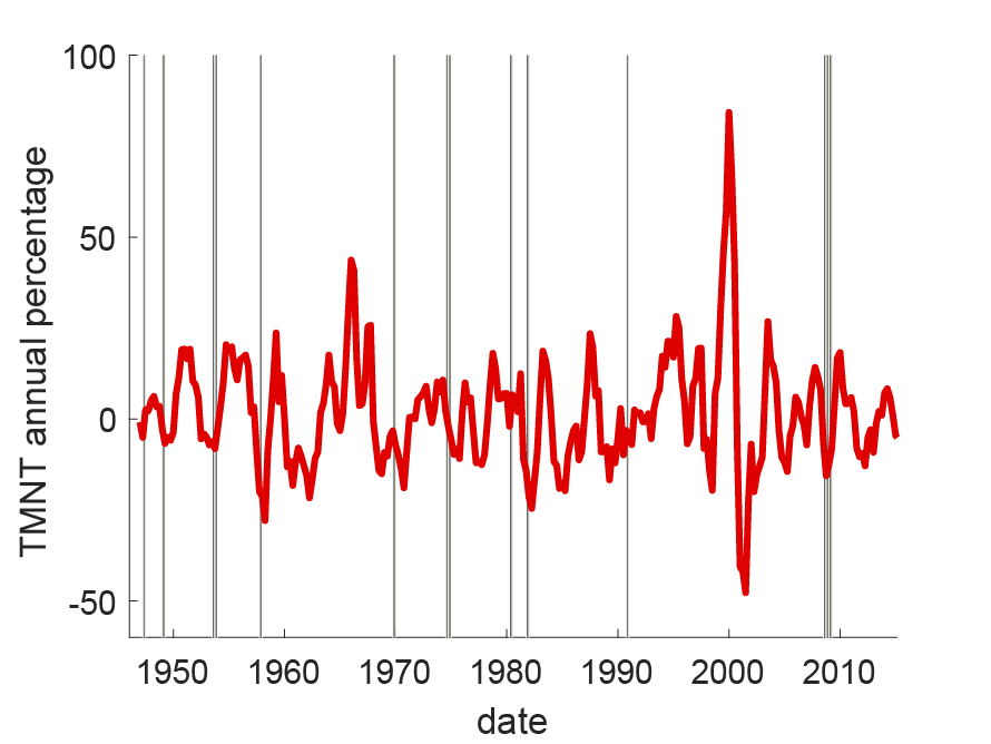
Fig. 1 plots the annual percentage returns of TMNT from 1947-2015. TMNT is the difference in value-weighted excess returns of portfolio T (quintile five) minus portfolio NT (quintile one) from a quintile sort of firms by tradability ratio. TMNT fluctuates mostly within a range of -50 to 50 percent, with a high of 84 percent in 2000, and a low of -48 percent in 2001. Recession dates, gray vertical lines, are defined as two consecutive quarters of decline in real U.S. GDP.
Business cycle effects dominate exchange rate effects
What role do exchange rates and economic growth play in the link between a firm's tradability and its stock returns? Table 3 answers this question. I regress quarterly portfolio returns on contemporaneous U.S. GDP growth and changes in the real dollar exchange rate (RER). The coefficients on these factors are labelled "GDP beta" and "RER beta" in the table, respectively. The real dollar exchange rate (in units of foreign currency per dollar) is computed as the GDP-weighted average of the real bilateral exchange rate between the U.S. and the foreign countries in the G7, and is available from 1957-2015.5
Table 3: Cyclicality of tradability-sorted portfolios
| $$NT$$ | 2 | 3 | 4 | $$T$$ | $$TMNT$$ | $$T1$$ | $$T2$$ | $$T3$$ | ||
|---|---|---|---|---|---|---|---|---|---|---|
| Full Sample: | ||||||||||
| 1. 1957-2015 | GDP beta | 2.16 | 2.34 | 2.29 | 2.46 | 3.84 | 1.69 | 3.39 | 3.78 | 4.37 |
| t-stat | 3.14 | 3.44 | 3.58 | 3.72 | 4.86 | 3.6 | 4.49 | 4.45 | 4.8 | |
| 2. 1957-2015 | GDP beta | 2.09 | 2.25 | 2.16 | 2.34 | 3.7 | 1.61 | 3.22 | 3.65 | 4.23 |
| t-stat | 3.16 | 3.47 | 3.52 | 3.68 | 4.91 | 3.45 | 4.5 | 4.44 | 4.79 | |
| RER beta | -0.16 | -0.2 | -0.27 | -0.26 | -0.32 | -0.16 | -0.36 | -0.29 | -0.31 | |
| t-stat | -1.22 | -1.43 | -2.44 | -2.08 | -1.91 | -2.97 | -2.18 | -1.86 | -1.64 | |
As shown in the table, firms with higher tradability have more cyclical asset returns (regression 1). In particular, returns of firms with the highest tradability (T) co-move almost twice as much with GDP growth than returns of firms with the lowest tradability (NT). GDP betas monotonically increase across the tradability-sorted portfolios, including the T sub-portfolios T1, T2, and T3, indicating that higher tradability, even among the highest tradability firms, implies more exposure to GDP fluctuations.
Regression 2 in the table shows the results after controlling for the real exchange rate exposure of the portfolios. GDP betas are little changed from the univariate regression 1. RER beta is insignificant for the low tradability portfolios, while it is significant and negative for the higher tradability portfolios. This makes intuitive sense as exports are negatively related to the value of the real dollar, leading high tradability firms to perform relatively worse than low tradability firms when the dollar appreciates. However, the business cycle effects appear to dominate the real exchange effects, both in economic and statistical significance, in explaining the difference in stock returns of tradability sorted portfolios. As observed in Table 2, high tradability firms significantly underperform low tradability firms during recessions and significantly outperform them during expansions. Put another way, it implies TMNT provided a hedge against recessions over the historical sample 1947-2015, where shorting it during recessions would have generated significant positive returns on average.
Using stock prices to predict the real exchange rate
The previous results showed that GDP growth and exchange rates have a contemporaneous and significant effect on the stock prices of tradability-sorted portfolios. At the same time, I show that the returns of TMNT, the difference in returns of U.S. firms with highest and lowest tradability, can predict future changes in the real dollar exchange rate.
The predictive regression results for the future change in the real exchange rate are shown in Figure 2, where columns one, two, and three plot the coefficients for TMNT, T, and NT, respectively (solid red line), along with the one and two standard error confidence intervals (the dashed and solid blue lines, respectively).
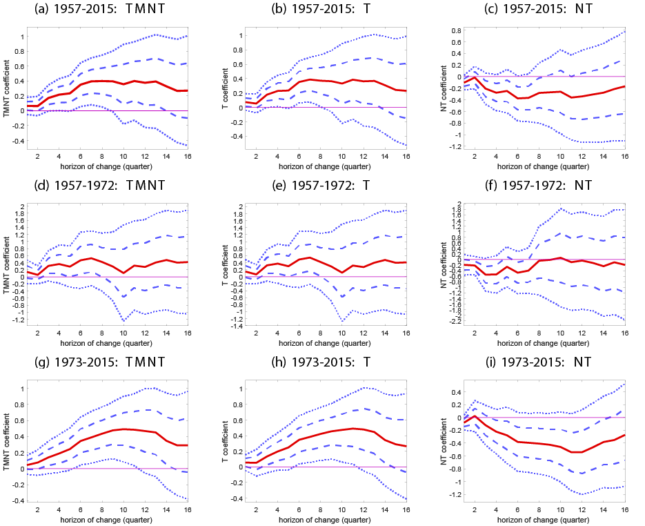
Fig. 2 shows the predictability of the real dollar exchange rate over the full sample (1957-2015), fixed exchange rate regime (1957-1972), and floating exchange rate regime (1973-2015) periods:
The first column plots the $$\beta_{h}$$ coefficient from regressing the forward-looking change in the exchange rate (foreign currency per dollar) on the quarterly return of the $$TMNT$$ portfolio, for $$h = 1$$ to 16 quarters. The second and third columns plot the $$\gamma_{T,h}$$ and $$\gamma_{NT,h}$$ coefficients from regressing on the return of the $$T$$ and $$NT$$ portfolio separately. The dashed lines represent one and two standard error confidence intervals.
Over the sample period 1957-2015 (row one), TMNT significantly predicts exchange rate changes over horizons of up to nine quarters ahead (panel a). The coefficient converges to 0.4 after seven quarters, implying a one percentage point increase in the quarterly return of TMNT leads to a 0.4 percent appreciation of the U.S. dollar seven quarters ahead. When the sample is split into the periods of fixed versus floating exchange rates (rows two and three), most of the predictability comes from the latter period (row three).
The results provide evidence of exchange rate predictability using stock returns. Rossi (2013) contains a recent survey of the empirical literature that traditionally uses economic models and macroeconomic variables in attempts to predict the real exchange rate. The random walk model consistently provides the toughest benchmark for these predictive models to beat. The advantage of using the stock returns of TMNT is that they are available at a higher frequency. Their forward-looking nature likely captures expected differential movements in the productivities of the tradable and non-tradable sectors in the economy, which should affect the real exchange rate.
References
Black, F., Jensen, M., Scholes, M., 1972. Studies in the theory of capital markets, Chapter The Capital Asset Pricing Model: Some Empirical Tests, pp. 79-121. Praeger.
Fama, E. F., French, K., 1993. Common risk factors in the returns on stocks and bonds. Journal of Financial Economics 33 (1), 3–56.
Newey, W. K., West, K. D., 1987. A simple, positive semi-definite heteroscedasticity and autocorrelation consistent covariance matrix. Econometrica 55 (3), 703–708.
Rossi, B., 2013. Exchange rate predictability. Journal of Economic Literature 51 (4), 1063–1119.
Stewart, R., Stone, J., Streitwieser, M., 2007. U.S. benchmark input-output accounts, 2002. Bureau of Economic Analysis 1, 1–20.
Tian, Mary (forthcoming). "Tradability of Output, Business Cycles, and Asset Prices," Journal of Financial Economics.
1. Senior Economist in the Division of Monetary Affairs of the Federal Reserve Board of Governors. I thank Shaghil Ahmed and Daniel Beltran for helpful comments. The views in this paper are solely the responsibility of the author and should not be interpreted as reflecting the views of the Board of Governors of the Federal Reserve System or of any other person associated with the Federal Reserve System. Return to text
2. Board staff calculations. International sales exposure is defined as the ratio of foreign sales to total sales, with high (low) exposure defined as being above (below) the 67th (33rd) percentile. Return to text
3. https://papers.ssrn.com/sol3/papers.cfm?abstract_id=1785027 Return to text
4. Annual firm-level sales data, segmented by industry, are from the Compustat historical segments database. Return to text
5. Data are from International Monetary Fund's International Financial Statistics (IMF IFS) database. Return to text
Tian, Mary (2018). "Differences in Stock Returns of U.S. Firms with High and Low Tradability," IFDP Notes. Washington: Board of Governors of the Federal Reserve System, January 2018, https://doi.org/10.17016/2573-2129.39.
Disclaimer: IFDP Notes are articles in which Board economists offer their own views and present analysis on a range of topics in economics and finance. These articles are shorter and less technically oriented than IFDP Working Papers.