Monetary Policy in a Forward-Looking Input-Output Economy*
Keywords: Inflation targeting, price-level targeting, intermediate goods
Abstract:
1 Introduction
Recent years have witnessed significant innovations in monetary policy as many central banks have adopted inflation targeting as their objective. Bernanke et al. (1999) and King (2005) have noted that, in general, those countries that have adopted inflation targeting were able to draw down inflation while experiencing economic performance that was favorable. These favorable results have motivated researchers to ask a number of questions regarding the design of monetary policy regimes, including: What goals should the government assign the central bank? What are the potential benefits if central banks were to commit to future actions based on current or future shocks to the economy? If such commitments are not realistic, how can policy be designed in order to closely approximate a commitment regime? How should policy be judged?
Researchers have made extensive use of New Keynesian macroeconomic models to study issues in monetary policy design. Most models assume that one production sector is subject to imperfect competition and sticky prices. These models can be seen as essentially equivalent to one-sector models in which a large number of differentiated final goods are produced by firms engaging in monopolistic competition.1 Within these models, the general conclusion has emerged that the central bank should seek to stabilize inflation in order to reduce household utility losses that occur over the business cycle.
When these policy studies are applied to the real world, inflation is typically identified with a change in some form of a consumer price index (CPI). However, one might ask: Is something like the CPI the best price index in guiding monetary policy? To pursue this matter further, Mankiw and Reis (2003) examine how characteristics of different sectors of the economy such as size, sensitivity to cyclicality, and sluggishness of price adjustment should enter into the price index of an inflation targeting central bank that wants to stabilize economic activity. They find that to reach this objective, a central bank may need to place a greater emphasis on nominal wages. This complements the studies by Erceg, Henderson, and Levin (2000) and Givens (2006), who also find that nominal rigidities in the labor market should lead central banks to target wages.
Huang and Liu (2005) develop a New Keynesian input-output model in which intermediate goods are used solely to produce consumption goods. Prices in both sectors are sticky. They show that including the inflation rate of intermediate goods prices improves the performance of simple instrument rules. However, many questions remain regarding monetary policy in a New Keynesian input-output model, such as: What are the characteristics of optimal policy in such an environment? Do policy recommendations from simpler one-sector models perform well in the more complex model? How should policy be designed if commitment to a loss function or instrument rules is not possible? Can discretionary policy be designed so that it approximates optimal policy? If there is uncertainty about parameter values characterizing the different sectors, how much of a difference do different central bank loss functions make?
I use the model from Huang and Liu (2005) with some minor extensions to examine in greater detail the characteristics of optimal commitment policies and the design of discretionary monetary policy when the input-output structure is characterized by sticky prices at both stages of production. I employ a second-order approximation to the household's utility function as a natural criterion by which to judge alternative policy prescriptions within the model. Under a parameterization consistent with the modern U.S. economy, I first study the equilibrium paths of key macroeconomic variables when a central bank can commit to a loss function based on the household's utility function. Compared to an otherwise equivalent sticky-price one-sector model, commitment in this two-sector model leads to a richer understanding of how policy makers should respond to shocks.
Next, under the more realistic assumption that central banks cannot commit to future policy actions or rules, I consider policy regimes that are pursued under discretion. I characterize monetary policy regimes by the loss function that they are assigned to minimize. I consider loss functions that include inflation targets and price-level targets in addition to other variables. I judge the performance of a regime by its effects on a model-consistent household loss function. I find that regimes that focus solely on CPI-based targets perform poorly. On the other hand, regimes that target price indices in both sectors perform the best among alternative inflation-targeting and price-level targeting regimes.
In related work on price-level targeting, Vestin (2006) shows that assigning a simple loss function that stabilizes a single price level like the CPI nearly replicates the commitment solution. In benchmark version of the richer input-output model, CPI price-level targeting no longer replicates the commitment solution in a standard one-sector New Keynesian model. Not only does a CPI price-level targeting regime perform worse than other price-level targeting regimes, its performance is nearly equaled by targeting inflation in both sectors instead of price levels. Furthermore, I show that a CPI price-level targeting regime that is calibrated in a one-sector world and then run in the true input-output world performs worse than the best inflation targeting regime.
I also show that targeting price indices in both sectors endows the regime with superior robustness properties. If there are potential misperceptions about the sources of shocks, a price-level targeting regime that includes prices of both sectors is very robust across a wide range of specifications of the sources of true shocks. I also show that regimes that only target one of the price indices perform much worse if actual parameter values differ from the assumed values when the loss function is set. Regimes that target both price indices perform very well over a wide range of parameter values that differ from the ones used in setting the initial policy regime.
The remainder of the paper proceeds in the following manner. Section 2 sets up the model used for the analysis. Section 3 examines the characteristics of the optimal policy under commitment within the model. Section 4 carries out a detailed analysis and comparison of various discretionary regimes. Section 5 examines the robustness properties of the different discretionary policy regimes. I examine the implications for policy of assuming a simple one-sector model, of misperceiving the sources of shocks, and parameter uncertainty. Section 6 considers the performance of various policy regimes under economies that differ from the benchmark economy in the importance of the intermediate goods sector. Section 7 concludes.
2 Model of an Input-Output Economy
The model I employ is in the tradition of New Keynesian models. I follow Huang and Liu (2005) in characterizing the production side of the economy as a production chain with sticky prices throughout.2 Specifically, differentiated final goods are produced using labor and a composite of differentiated intermediate goods. Both sectors exhibit sticky prices. However, I model the policy side of the economy very differently than in Huang and Liu (2005). I assume that the government assigns goals to an independent central bank in the form of an intertemporal loss function. The central bank acts to minimize this loss function.
2.1 Households
The economy is populated by an infinite number of identical households. These households maximize expected lifetime utility, which is given by
E![\displaystyle _{0}\left\{ \sum_{t=0}^{\infty}\beta^{t}\left[ u\left( C_{t}\right) -v\left( N_{t}\right) \right] \right\} .](img5.gif) |
(1) |
Households take wages as given and are assumed to provide labor to all firms in the economy. In this paper I assume that
![\displaystyle C_{t}\equiv\left[ \int_{0}^{1}y_{ft}\left( i\right) ^{\left( \the... ...ight) /\theta_{ft}} di\right] ^{\theta_{ft}/\left( \theta _{ft}-1\right) }%](img9.gif) |
(2) |
where
2.2 Firms
On the production side there are two sectors, each consisting of a continuum of firms producing differentiated goods. The first sector produces goods that households consume, while the second sector produces intermediate goods that are needed to produce the final goods. All firms are price takers in their input markets. I assume a competitive labor market in which one wage obtains in the entire economy. Firms engage in monopolistic competition in each sector. I assume that firms have the opportunity to adjust their prices via the standard Calvo framework.
2.2.1 Final Goods
The final goods firms have access to a constant-returns-to-scale Cobb-Douglas production function with labor-augmenting technology,
| (3) |
where
![\displaystyle Y_{mt}\left( i\right) \equiv\left[ \int_{0}^{1}y_{mt}\left( i,j\r... ...1\right) /\theta_{mt}} dj\right] ^{\theta _{mt}/\left( \theta_{mt}-1\right) }](img18.gif) , , |
(4) |
where
Final goods firms can adjust their prices with probability
![]() each period. When they are able, they set a price that maximizes expected discounted profits. Each firm meets the demand for its goods given its stated price. The markup that
firms charge varies as the elasticity of substitution varies. This can be seen as a proxy for any change in the economic environment that affects the markup that monopolistic firms could charge above their marginal cost in a hypothetical flexible price environment. For example, if households were
to substitute differentiated goods for one another more readily due to preference changes, increased varieties of goods, or any other reason, firms would experience a shock on the markup that they could charge over their marginal costs.3 The profit-maximization problem can be represented as
each period. When they are able, they set a price that maximizes expected discounted profits. Each firm meets the demand for its goods given its stated price. The markup that
firms charge varies as the elasticity of substitution varies. This can be seen as a proxy for any change in the economic environment that affects the markup that monopolistic firms could charge above their marginal cost in a hypothetical flexible price environment. For example, if households were
to substitute differentiated goods for one another more readily due to preference changes, increased varieties of goods, or any other reason, firms would experience a shock on the markup that they could charge over their marginal costs.3 The profit-maximization problem can be represented as
where
2.2.2 Intermediate Goods
The intermediate goods firms face an optimization problem similar to the one faced by final goods producers. Intermediate goods firms have access to a constant-returns-to-scale production function of the form
| (6) |
where
2.3 Government
The government serves two purposes in this model. First, it assigns a loss function to an independent central bank. The central bank sets the nominal interest rate to achieve its assigned goals. I assume that the central bank can react to and affect state variables in the current period.4 I solve for Markov Perfect equilibria under the assumption that the central bank does not engage in complicated strategies to support other possible equilibria in a dynamic game with households.
The second task of the government is to tax households and provide subsidies to firms so that the steady-state equilibrium is not distorted due to the inefficiencies arising from monopolistic competition. I assume that the government does this via lump-sum taxes and always maintains a balanced budget. A natural extension of this setup is to study how more realistic fiscal and monetary policies can affect one another in this environment. This interaction may affect the loss function that the government would assign to the central bank.5 I ignore these possible complications for the remainder of the paper and leave their study for future research.
2.4 Reduced-Form Model
I log linearize the model using log deviations from a hypothetical efficient equilibrium (the equilibrium that would obtain if prices were flexible and there were no elasticity-of-substitution shocks).6 I define the natural rates or values as those values that would arise in the efficient equilibrium. The log-linear approximation to the model will be valid as long as shocks to the system are sufficiently small relative to the size of the state variables. Table 1 lists the key variables and symbols.
The intertemporal IS equation is obtained from the household's first-order condition. Its log-linearized version is given by
| (7) |
where
| (8) |
where
and
The cost-push shocks, ![]() for
for
![]() , are reduced-form expressions of fluctuations in the time-varying elasticities of substitution of the differentiated goods. I assume that each cost-push shock is
given by
, are reduced-form expressions of fluctuations in the time-varying elasticities of substitution of the differentiated goods. I assume that each cost-push shock is
given by
| (11) |
where


The final goods Phillips curve in this setting gives an indication of why the coefficient of the output gap in a fully specified, reduced-form empirical Phillips curves might be smaller than otherwise expected if the intermediate goods sector is important. The coefficient for this term in the
final goods Phillips curve, given by
![]() , decreases with
, decreases with ![]() (while the
coefficient of the relative price term increases at the same time). Thus, in the input-output model, higher levels of importance of the intermediate goods sector have similar effects on the coefficient of the output gap as parameter values in a one-sector model that imply higher degrees of
strategic complementarities (e.g., see Kimball, 1995, and Woodford, 2003).7
(while the
coefficient of the relative price term increases at the same time). Thus, in the input-output model, higher levels of importance of the intermediate goods sector have similar effects on the coefficient of the output gap as parameter values in a one-sector model that imply higher degrees of
strategic complementarities (e.g., see Kimball, 1995, and Woodford, 2003).7
In order to judge households' preferences over different policy options, I find it useful to use a second-order Taylor approximation to the household utility function. For the present model, this is given by:
 E E t.i.p. t.i.p. |
(13) |
where
"t.i.p" represents terms independent of policy, and
When solving the model I treat
![]() as the instrument of the central bank. This is an innocuous simplification since the interest rate does not appear in the objective function of the central bank and the IS
equation is not a constraint in the central bank's optimization problem. Since the nominal interest rate can be uniquely determined through the IS curve, I obtain the solution in which the nominal interest rate is the policy instrument. I compute price levels using the identity,
as the instrument of the central bank. This is an innocuous simplification since the interest rate does not appear in the objective function of the central bank and the IS
equation is not a constraint in the central bank's optimization problem. Since the nominal interest rate can be uniquely determined through the IS curve, I obtain the solution in which the nominal interest rate is the policy instrument. I compute price levels using the identity,
![]() for
for
![]() , where
, where ![]() is the log-deviation in the price level from
its initial value as determined in a steady state. I represent the structural equations of the economy as
is the log-deviation in the price level from
its initial value as determined in a steady state. I represent the structural equations of the economy as
where
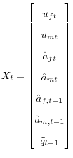 ,
,  ,
, 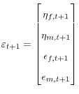 .
.3 Optimal Policy with Commitment
In this section I study policy under the assumption that the central bank can be assigned a loss function that is derived from the household utility function, and that it can commit to future actions. This policy regime provides a benchmark with which to compare the results of discretionary monetary policy. Additionally, the characteristics of impulse responses to shocks and long-run outcomes under the commitment solution provide further means of judging the desirability of particular policy prescriptions.
In state-space form the policy period loss function is given by
where
The matrix of loss coefficients,
E . . |
(18) |
Without loss of generality, I have multiplied the loss function by
Under commitment, the central bank solves the standard Lagrangian
 |
(19) | |
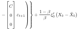 , , |
where I have used the law of iterated expectations to consolidate the Lagrangian. I have written the vector of Lagrangian multipliers relating to the forward-looking variables as
3.1 Benchmark Calibration of the Model
To complete the model setup, in this section I describe the parameter values that characterize the benchmark economy. The assumption of log utility in consumption implies that ![]() . I
set
. I
set
![]() , which implies that the annual real interest rate in the steady state is approximately 4 percent, given that I interpret a time period to be a quarter. Consistent with Blinder et
al. (1998) and Carlton (1986), I set the average price contract equal to a year, which means setting
, which implies that the annual real interest rate in the steady state is approximately 4 percent, given that I interpret a time period to be a quarter. Consistent with Blinder et
al. (1998) and Carlton (1986), I set the average price contract equal to a year, which means setting
![]() and
and
![]() .9 The steady-state elasticities
of substitution for the differentiated goods,
.9 The steady-state elasticities
of substitution for the differentiated goods,
![]() and
and
![]() , are set to 10, which implies a steady-state markup of 11 percent.
, are set to 10, which implies a steady-state markup of 11 percent.
The intermediate goods sector is the crucial feature of the paper's analysis, and therefore it is important to be careful in setting ![]() , the parameter that indexes its importance.
Given that I consider a constant-returns-to-scale Cobb-Douglas production function, I can interpret
, the parameter that indexes its importance.
Given that I consider a constant-returns-to-scale Cobb-Douglas production function, I can interpret ![]() as the share of total input costs of intermediate goods. Jorgenson et al. (1987)
and Hornstein and Praschnik (1997) examine the role of intermediate inputs in the production in final goods. Their results suggest that
as the share of total input costs of intermediate goods. Jorgenson et al. (1987)
and Hornstein and Praschnik (1997) examine the role of intermediate inputs in the production in final goods. Their results suggest that ![]() could be reasonably interpreted as falling in
the interval
could be reasonably interpreted as falling in
the interval
![]() . For the benchmark calibration, I assume that
. For the benchmark calibration, I assume that
![]() , which puts the benchmark economy in the middle of the range of reasonable values.10 Following the analysis of the benchmark economy, I examine the consequences of setting
, which puts the benchmark economy in the middle of the range of reasonable values.10 Following the analysis of the benchmark economy, I examine the consequences of setting ![]() to be greater or lower
than this value.
to be greater or lower
than this value.
I set the AR(1) coefficients for technology shocks to
![]() . The standard deviations of the innovations to productivity shocks are set to 0.02. These values are consistent with empirical studies that show productivity shocks to be small, but highly persistent (for example, see Cooley and Prescott, 1995, Kim, 2000, and Huang and Liu, 2005). There is less agreement on the characterization of cost-push
shocks. For simplicity, I assume that the cost-push shocks are purely transitory by setting
. The standard deviations of the innovations to productivity shocks are set to 0.02. These values are consistent with empirical studies that show productivity shocks to be small, but highly persistent (for example, see Cooley and Prescott, 1995, Kim, 2000, and Huang and Liu, 2005). There is less agreement on the characterization of cost-push
shocks. For simplicity, I assume that the cost-push shocks are purely transitory by setting
![]() , and set the standard deviations of their white noise shock components to 0.02. Considering purely transitory shocks simplifies the analysis and allows for an easy comparison with other purely forward-looking studies.11 My calibration of the standard deviation of the cost-push shocks is similar to Walsh (2003b) and Jensen (2002).
, and set the standard deviations of their white noise shock components to 0.02. Considering purely transitory shocks simplifies the analysis and allows for an easy comparison with other purely forward-looking studies.11 My calibration of the standard deviation of the cost-push shocks is similar to Walsh (2003b) and Jensen (2002).
3.2 Optimal Policy under Commitment in the Benchmark Economy
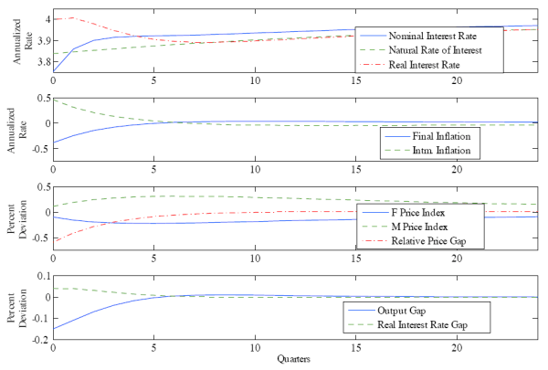
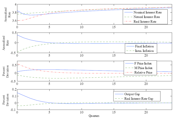
The equilibrium dynamics following a one-standard-deviation shock to productivity in the final goods sector are given in Figure 1, while the dynamics after a similar shock in the intermediate goods sector are given in Figure 2.
The bottom panel of Figure 1 shows the behavior of the real interest rate gap and output gap, both of which indicate the stance of monetary policy. Contractionary monetary policy is undertaken in response to the productivity shock as indicated by the positive real interest rate gap. The contractionary policy move is accompanied by a decrease in the absolute level of the equilibrium nominal interest rate, which slowly rises thereafter.
The second panel of Figure 1 shows the behavior of inflation in the two sectors in response to a productivity shock in the final goods sector. The productivity shock induces inflation rates in each sector to move in opposite directions. The real marginal cost gaps in the two sectoral Phillips curves open a window to the transmission mechanism for shocks affecting inflation in the two sectors. As shown in (12), the productivity shock directly affects the relative price gap. Equations (9) and (10) show that the relative price gap pushes the real marginal cost gaps, and hence inflation, in opposite directions in the two sectors. Furthermore, the intermediate goods sector is more sensitive to productivity shocks than is the final goods sector, and therefore intermediate goods inflation will be greater in magnitude unless the central bank acts to alleviate this effect.
The central bank must account for the different sensitivities of the two sectors to the shock and to the nominal interest rate in order to bring about the optimal path of the nominal interest rate. After a productivity shock in the final goods sector, the central bank relieves the excess pressure on the intermediate goods sector through contractionary policy, inducing slightly greater deflation in the final goods sector, and less inflation in the intermediate goods sector. The balancing of inflation across the two sectors allows for a more efficient distribution of resources within and across the sectors. The third panel shows that in the long run the price levels are brought back to their original levels. The price level's long-run neutrality provides a reason to believe that some form of price-level targeting in this environment may prove to be optimal under discretion.
Figure 2 shows that a one-standard-deviation shock to the productivity of the intermediate goods sector leads to similar conclusions; one must simply reverse all of the directions in which the variables move with one notable exception. The model predicts that under optimal policy the central bank initially decreases the nominal interest rate regardless of the sector from which the productivity shock arises. The nominal interest rate decreases after productivity shocks in both sectors despite the fact that policy is contractionary following a final goods productivity shock and expansionary following an intermediate goods productivity shock. The seemingly disjoint behavior between the nominal interest rate and the policy stance occurs because the equilibrium real interest rate always falls below its steady state value following productivity shocks, though by different amounts depending on the sector in which the shock arises.
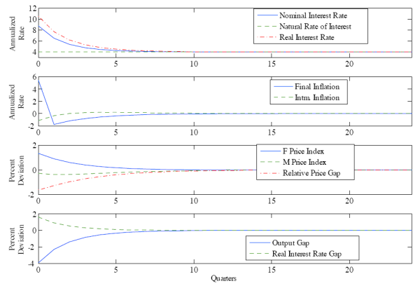
Figure 3 displays the equilibrium dynamics following a cost-push shock in the final goods sector. If the central bank were to engage in neutral policy (zero real-interest-rate gap), both sectors would experience inflation; however, inflation in the final goods sector would be extremely high. The central bank engages in contractionary policy to reduce inflation in both sectors, balancing the higher sensitivity of inflation in the intermediate goods sector to the nominal interest rate with the large initial effect on final goods inflation from the cost-push shock.
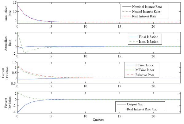
Figure 4 shows that the impulse responses to a cost-push shock in the intermediate goods sector retain the same qualitative characteristics as those in Figure 3, but carry the opposite sign in inflation rates and price levels. Once again both sectors experience inflationary pressure, with the intermediate goods sector experiencing a stronger initial push in this instance. Just as in the previous case, the central bank pursues contractionary policy in response to the cost-push shock. Nevertheless, since inflation in the intermediate goods sector is more sensitive to the nominal interest rate and is affected more by the cost-push shock, the central bank will set the magnitude of its response differently than when responding to a cost-push shock in the final goods sector.
4 Policy under Discretion
Under the more realistic assumption that central banks cannot commit to future actions, I study policy regimes that minimize assigned loss functions under discretion.12 Moreover, I focus on regimes that admit simple loss functions since they are easier to communicate to the public in a transparent and understandable way. Inflation and price-level targeting have been leading candidates in the study of the performance of simple loss functions under discretion. A next logical step would be to combine inflation and price-level targeting into a hybrid regime that includes targets of both kinds in the loss function. However, in results not reported, I find that there is no discernible difference in performance between simple price-level targeting and a hybrid scheme that includes both inflation and price-level targets. Some studies such as Walsh (2003b) and Néssen and Vestin (2005) have found that alternative classes of regimes, such as "speed limit" policies (regimes that include changes in the output gap) and average inflation targeting perform better than pure price-level or inflation targeting regimes, but only when there is persistence in inflation.13 I therefore concentrate on simple price-level and inflation targeting regimes.
I use the household loss function as the model-consistent metric for assessing the performance of different regimes. Furthermore, I use the household losses under the optimal commitment policy as a reference for the discretionary policy regimes. The idea that the assigned loss function may differ from the household loss function has been introduced into many studies following the initial suggestion in Barro and Gordon (1983) and further development in Rogoff (1985). I rank candidate inflation and price-level targeting regimes by their implied effects on expected household utility.
4.1 Characterization of Policy Regimes
Policy regimes are defined by the type of loss function that is assigned to the central bank. Loss functions take the same general form as the household loss function, but the target variables and weights are determined by the government. I define inflation targeting regimes as having the common
feature that inflation rates enter the assigned loss function as target variables, regardless of additional variables that may enter the loss function. The period loss function for an inflation targeter takes the same form as (16) and (17), where
![]() is replaced by a set of weights that is assigned by the government and represented by
is replaced by a set of weights that is assigned by the government and represented by
Within this class of inflation targeting regimes,pure discretion (PD) is the regime in which the central bank is assigned the household loss-function weights (given in
![]() ). I consider three additional inflation targeting regimes whose weights do not arise directly from the household utility function: CPI inflation targeting (CIT), intermediate
goods inflation targeting (PIT), and dual inflation targeting (DIT). Under CIT, the weight on intermediate goods inflation,
). I consider three additional inflation targeting regimes whose weights do not arise directly from the household utility function: CPI inflation targeting (CIT), intermediate
goods inflation targeting (PIT), and dual inflation targeting (DIT). Under CIT, the weight on intermediate goods inflation,
![]() is set to zero, as is the weight for final goods inflation,
is set to zero, as is the weight for final goods inflation,
![]() under PIT. Under DIT both weights are positive.
under PIT. Under DIT both weights are positive.
I follow Svensson (1999a) and consider a price-level targeting regime to be characterized by loss functions of a similar form as above in which squared deviations of the price-level from some target value replace inflation terms. I consider three analogous price-level targeting regimes: CPI
price-level targeting (CPT), intermediate goods price-level targeting (PPT), and dual price-level targeting (DPT). Under CPT the weight on the price level of intermediate goods,
![]() is set to zero, as is the weight on the price level of final goods,
is set to zero, as is the weight on the price level of final goods,
![]() under PPT. Under DPT both coefficients are positive.
under PPT. Under DPT both coefficients are positive.
4.2 Policy Regime Comparisons
To compare the relative performances of the various discretionary policy regimes, I compute the expected utility losses from their respectively induced equilibrium paths. In each case I report the implied household loss as a percentage of quarterly steady-state output and as a percent deviation of the household loss compared to the household loss under the hypothetical optimal commitment policy (COM). It is important to note that this methodology differs from that utilized in other studies that compare discretionary policy regimes using ad hoc loss functions as the metric (for example, see Walsh, 2003b).
Since assigned loss functions do not come from the model, some care must be taken in setting the weights on the target variables in the loss functions. Often in the literature weights are arbitrarily chosen. These weights are then used across regimes in order to rank the regimes' effectiveness at minimizing the overall loss function. However, proceeding in such a manner may bias the test in favor of one of the regimes due to accidentally favorable weights. Moreover, one would not know which regimes would receive a favorable bias. Some authors do include a range of weights, which alleviates this problem to some degree. Nevertheless, with a large parameter space, doubt can still remain as to hidden biases. In order to circumvent this problem, I use numerical methods to find the joint set of weights for each policy regime which then leads to the minimum household loss for that regime type, subject to the constraint that each weight be nonnegative.14
Each period the central bank minimizes its assigned loss function subject to (15). To solve for a Markov Perfect equilibrium, I apply standard dynamic programming techniques. This linear-quadratic setup leads to a quadratic value function, given by
| (20) |
The scalar
| (21) | ||
![\displaystyle =\left( 1-\beta\right) \min _{\widetilde{c}_{t}}\left\{ L_{t}+\b... ...}^{\prime}V_{t+1}X_{t+1}+\frac{\beta}{1-\beta}z_{t+1}\right] \right\} \text{.}](img130.gif) |
Table 2 reports the optimal target weights for the different regimes as well as the expected household utility losses. I report the unconditional household loss as a percentage of permanent quarterly steady-state consumption, calculated as
![\displaystyle \bar{C}=100\frac{\text{E}\left[ \mathcal{L}% ^{regime}\right] }{u_{C}\left( \bar{C}\right) \bar{C}}\text{,}%](img131.gif)
The optimal weights for a dual inflation targeting regime are close to the weights in the household loss function itself (assigned in PD and COM). The dual inflation targeting regime places more relative weight on inflation in the intermediate goods sector and on the real marginal cost in the intermediate sector than does the household loss function. Regimes that target both price indices put more weight on final goods prices than on intermediate goods prices.
Within both inflation targeting and price-level targeting regimes, targeting both indices produces the best results.15 Exclusively targeting the final goods index produces the worst results in each regime class. The class of price-level targeting regimes outperforms the class of inflation targeting regimes.16 However, the difference between the best inflation targeting regime, DIT, and the worst price-level targeting regime, CPT, is small.
|
|---|
These results obtain in a model in which all sectors are buffeted by both productivity and cost-push shocks. What if the economy has the input-output structure, but is only buffeted by a subset of the shocks posited in the benchmark economy? I study four alternative shock scenarios in which there are only productivity shocks, cost-push shocks, final goods shocks, and intermediate goods shocks. I assume that policy makers understand the true shock processes and choose the optimal loss function weights given the true shock processes. Table 3 reports the losses for the discretionary regimes that use loss functions crafted under the four alternative true-shock-source scenarios (each column contains the minimal losses that the various regimes can attain under the conditional shock mechanism). The losses are reported as a percent of permanent quarterly steady-state consumption given the particular assumption of the source of shocks.
|
|---|
Table 3 shows that the same general patterns of policy effectiveness obtain under various assumptions of the sources of shocks.17 The main difference is that sometimes only targeting intermediate good price inflation or price levels proves less effective. Similar to the benchmark model, price-level targeting generally outperforms inflation targeting, targeting prices in both sectors outperforms targeting prices in only one sector, and dual price-level targeting is always the best-performing regime. In fact, dual price-level targeting performs nearly as well as the optimal commitment policy.
5 Robustness of Discretionary Policies
In the previous section, I assumed that the government was aware of the correct model and correctly perceived the different shocks that hit the economy when formulating the loss function for the central bank. However, given the uncertainty that governments and central banks face in determining the correct model and the sources of shocks, it is worthwhile to explore the following questions: What happens if the government erroneously bases its policy based on the assumption of a one-sector economy? What happens if policy makers do not correctly identify the sectors from which shocks arise? How robust are the results to parameter values that differ from those on which the original policy is based (either due to mismeasurement or changes in the structure of the economy following the adoption of the policy regime)?
In this section I examine these three general areas of concern about policy robustness. First I examine the consequences of the government incorrectly basing policy on a once-sector model. I then consider the implications for household losses when the government misperceives the sources of shocks to the economy. Finally I consider the consequences when the parameters characterizing the importance of intermediate goods to final goods production and price stickiness in the two sectors differ from those used in the policy calibration.
5.1 Implementation of Policies from a Simple One-Sector Model
Suppose the government assigns loss functions based on a one-sector model, despite the underlying reality of the input-output model. Within the one-sector framework I consider two competing regimes: (C)IT (inflation targeting), and (C)PT (price-level targeting), in which I identify inflation and price-level targets with consumer price indices. I calculate the optimal weights for inflation and price-level targeting in the one-sector world. The loss functions are assigned to the central bank, which minimizes the loss functions subject to (15) in the true economy. I report the losses that households would experience in the benchmark economy under these one-sector-based policies in Table 4 (these losses are directly comparable to those in Table 2).
|
|---|
Table 4 confirms that the order of performance of price-level and inflation targeting regimes does not change when they are incorrectly based on a one-sector model. However, a comparison of these results with those in Table 2 shows that carrying policy prescriptions straight over from the one-sector model can lead to unintended outcomes. The one-sector (CPI) inflation targeting prescription performs worse than the other inflation targeting regimes when implemented within the full input-output model. Furthermore, not only does (C)PT perform worse than the other price-level targeting regimes, it performs worse than the dual inflation targeting regime, DIT. Thus, it is possible to design an inflation targeting regime within the input-output model that outperforms the optimal price-level targeting regime that has been carried over from the one-sector model.
5.2 Policy Robustness under Misperceptions of Shocks
Suppose now that the central bank realizes that the input-output model represents a more accurate view of the world, but constructs its policy reaction function based on misperceptions regarding shocks. I examine the implications for household losses if the central bank cannot distinguish the sector or type of shock that hits the economy. Specifically, I allow the government to choose loss-function coefficient values based on its belief regarding the source of shocks. I then determine the unconditional expected household losses when the policy based on a misperception of shock sources is used within the benchmark economy. Table 5 reports the losses for each regime as a percentage of the permanent quarterly steady-state consumption, which means that these losses can be compared directly to those reported in Table 2. In the column labeled "Benchmark," I have reproduced the losses from Table 2 in which the correctly formulated benchmark loss functions are run in the benchmark world.
|
|---|
The central bank's performance deteriorates when its misperception of the sources of shocks leads it to put too much weight on stabilizing prices in either of the two sectors (not only relative to prices in the other sector, but also relative to the output gap and intermediate goods real marginal cost gap). Under the assumption of only final goods shocks the weights for DIT are especially affected. Under the assumption of only intermediate goods shocks, the weights in CIT, DIT, and CPT lead to poor performances in the benchmark model.
The most robust result that emerges from this exercise is that even if the policy makers misperceive the sources of shocks to the economy, they minimize their losses by choosing a DPT regime. Even when the DPT loss function is formulated under misperceptions, it outperforms not only all of the other regimes that were formed under the same misperception of shocks, but also almost all of the other regimes that were formulated under a correct perception of the sources of shocks.
Suppose, instead, that the government erroneously assumes that shocks occur as posited in the benchmark model and uses the loss functions based on the benchmark model in economies with different sources of shocks. I examine the household losses under the benchmark-formulated discretionary regimes in each of the four alternative economies: only final goods shocks, only intermediate goods shocks, only productivity shocks, and only cost-push shocks. Table 6 reports the losses as the percent of permanent quarterly steady-state consumption (where the steady state consumption is formulated for an economy with the conditional shock structure). The losses in each column can be compared directly to the corresponding columns in Table 3.
|
|---|
Once again, the dual price-level targeting regime clearly outperforms all of the other specifications, and, with a few exceptions, price-level targeting generally outperforms inflation targeting. Dual inflation targeting always outperforms single-sector inflation targeting of either type. These two exercises jointly show that the policy makers can best avoid unpleasant ex post policy results when there are potential misperceptions about shocks by targeting prices in both sectors, especially when they target price levels instead of inflation rates.
Shock misperceptions can make important differences regarding the actual performance of policies that are thought ex ante to be good. Assuming that shocks hit both sectors and are both of the labor-augmenting productivity type and cost-push shock type prevents the central bank from being exposed to the extreme risk that can occur with policies based on the assumption of only intermediate goods shocks are implemented in a benchmark world. Benchmark-based regimes experience their highest decreases in performance when they are implemented in worlds in which there are only intermediate goods shocks or only productivity shocks (as judged by the percentage increase in loss compared to when they are calibrated and run according to the correct perceptions of shocks). If the DIT regime is set in the benchmark world, it is fairly robust (meaning that it never occupies a lower relative rank to other policies in non-benchmark worlds). However, it is much less robust when formulated on the assumption of restricted sets of shocks. One clear result emerges: DPT always performs well, no matter what set of shocks were assumed to be true when formulating its loss function and no matter what the true world is in which it is implemented.
5.3 Policy Robustness to Parameter Changes
Besides model and shock uncertainty, policy makers must contend with parameter uncertainty. In this model, the intensity of the use of intermediate goods and the price stickiness in the two sectors constitute key features relevant for policy analysis. In order to understand the effect of
uncertainty regarding the intensity of use of intermediate goods in the production process, I examine the losses that occur as ![]() ranges over values that differ from the value used to
formulate policy. In this and subsequent robustness exercises, I assume that the stochastic nature of the shocks does not change across these different environments. I also assume that the central bank can correctly identify the source of the shocks. To accomplish this, I first find the optimized
loss-function coefficients for the various policy regimes based on the benchmark calibration. I then run this policy in economies in which the value of
ranges over values that differ from the value used to
formulate policy. In this and subsequent robustness exercises, I assume that the stochastic nature of the shocks does not change across these different environments. I also assume that the central bank can correctly identify the source of the shocks. To accomplish this, I first find the optimized
loss-function coefficients for the various policy regimes based on the benchmark calibration. I then run this policy in economies in which the value of ![]() differs from the benchmark
value.
differs from the benchmark
value.
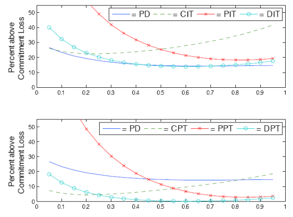
Figure 5 reports the losses of benchmark discretionary regimes relative to the conditional optimal commitment policy as the true or post-policy value of ![]() varies from 0 to 1. The top panel displays the results for the inflation targeting regimes, while the bottom panel shows the results for the price-level targeting regimes. PD differs from
the other policies in that its weights implicitly change as the parameter values change.18 PD is plotted in both panels to facilitate an easier comparison
of the inflation and price-level targeting regimes. DPT remains the best regime for a very large portion of the parameter space. It becomes the second-best regime if
varies from 0 to 1. The top panel displays the results for the inflation targeting regimes, while the bottom panel shows the results for the price-level targeting regimes. PD differs from
the other policies in that its weights implicitly change as the parameter values change.18 PD is plotted in both panels to facilitate an easier comparison
of the inflation and price-level targeting regimes. DPT remains the best regime for a very large portion of the parameter space. It becomes the second-best regime if ![]() turns out to be
less than 0.25. CPT proves to be much more robust than PPT, especially at lower values of
turns out to be
less than 0.25. CPT proves to be much more robust than PPT, especially at lower values of ![]() . Among the inflation-targeting regimes, DIT exhibits the best robustness. CIT performs especially well if
. Among the inflation-targeting regimes, DIT exhibits the best robustness. CIT performs especially well if ![]() turns out to be lower than expected, while PIT
performs well if
turns out to be lower than expected, while PIT
performs well if ![]() is higher than expected.
is higher than expected.
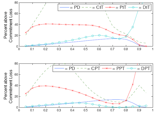
Figure 6 displays the results if price stickiness turns out to be different than expected (but still equal in the two sectors).19 If price stickiness turns out to be lower than expected, all four regimes that target either prices or inflation in only one sector perform worse than the dual targeting regimes. DIT performs very well only if price stickiness turns out to be less than the values used to calibrate the loss function. DPT performs well over the entire range and proves to be the most robust regime with respect to uncertainty in price stickiness.
These results support the idea that dual price-level targeting under discretion allows the central bank to achieve results similar to an optimal commitment regime in forward-looking New Keynesian models with little risk due to uncertainty in these parameter values. However, while many modern central banks can be characterized as operating within a framework similar to CIT, no modern central bank targets price levels. Given the lack of experience with price-level targeting20, a move to something like DIT first, and then to DPT may provide a smoother path towards the optimally performing regime.21 This would allow central banks to gain experience in monitoring and reacting to intermediate goods price indices while they prepare to switch to price-level targeting.
6 The Importance of Intermediate Goods
Though the benchmark economy serves as a good basis by which to judge an economy similar to that of the United States today, it is natural to ask how these results would be different if the intermediate goods sector were more or less important. This question is important for at least two
reasons. First, economies at different stages of development may utilize intermediate goods with different levels of intensity. Hanes (1996) has documented the fact that modern consumption goods in the U.S. pass through more stages of production today than they did in earlier times.22 Second, economies at similar stages of development may nevertheless differ in their use of intermediate inputs, and therefore would be characterized by
different values of ![]() .
.
6.1 High Importance of Intermediate Goods
For an economy that exhibits an intense use of intermediate goods, I assume the same parameterization as the benchmark model, except that I now set
![]() . This corresponds to the upper end of the range for
. This corresponds to the upper end of the range for ![]() in the
United States, and a correspondingly high importance of the intermediate goods sector in the production process of final goods. Table 7 reports the weights for the optimized loss coefficients, the loss as a percentage of steady-state output, and the losses relative to the optimal commitment policy
in the right-most column.
in the
United States, and a correspondingly high importance of the intermediate goods sector in the production process of final goods. Table 7 reports the weights for the optimized loss coefficients, the loss as a percentage of steady-state output, and the losses relative to the optimal commitment policy
in the right-most column.
Once again DPT is the top performing regime. However, the weight placed on the price level of the intermediate good has increased substantially. Furthermore, PPT is now very close to DPT and much better than the remaining regimes. CPT is actually marginally worse than DIT. These results come as
no surprise since a larger value for ![]() means that the intermediate goods are more important in the production process. DIT's ability to outperform other inflation targeting regimes when
means that the intermediate goods are more important in the production process. DIT's ability to outperform other inflation targeting regimes when
![]() is high reinforces the idea that it serves as a good intermediate regime.
is high reinforces the idea that it serves as a good intermediate regime.
|
|---|
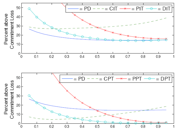
I repeat the earlier robustness analysis and plot the relative losses under these regimes for different true or post-policy values of ![]() in Figure 7. These results complement the
results obtained for policies crafted in the benchmark economy. Except for very low values of
in Figure 7. These results complement the
results obtained for policies crafted in the benchmark economy. Except for very low values of ![]() , dual price-level and inflation targeting continue to be robust, outperforming other
regimes in each class. Compared to the benchmark case, CIT and CPT demonstrate more robustness than they did under the benchmark calibration. On the other hand, PIT and PPT perform very poorly if
, dual price-level and inflation targeting continue to be robust, outperforming other
regimes in each class. Compared to the benchmark case, CIT and CPT demonstrate more robustness than they did under the benchmark calibration. On the other hand, PIT and PPT perform very poorly if ![]() is significantly lower than expected.
is significantly lower than expected.
6.2 Low Importance of Intermediate Goods
In order to consider an economy that exhibits a low intensity of intermediate goods use, I assume that
![]() . Table 8 reports the results the loss function weights and implied household losses under this assumption. Again, DPT is not only the top performer, but very nearly replicates
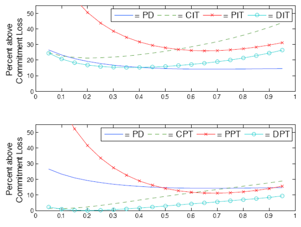
the performance of the optimal commitment solution. CPT performs much better than all other regimes and nearly as well as DPT. Targeting only intermediate prices proves to be less successful, with PPT performing worse than both PD and CIT. Figure 8 shows that the dual-targeting regimes continue to
exhibit good robustness properties when the true or post-policy values of
. Table 8 reports the results the loss function weights and implied household losses under this assumption. Again, DPT is not only the top performer, but very nearly replicates
the performance of the optimal commitment solution. CPT performs much better than all other regimes and nearly as well as DPT. Targeting only intermediate prices proves to be less successful, with PPT performing worse than both PD and CIT. Figure 8 shows that the dual-targeting regimes continue to
exhibit good robustness properties when the true or post-policy values of ![]() turn out to be much higher than an assumed low value. DPT is the best of all regimes, while DIT performs
better than the other inflation-targeting regimes.
turn out to be much higher than an assumed low value. DPT is the best of all regimes, while DIT performs
better than the other inflation-targeting regimes.
|
|---|
7 Conclusion
In this paper I have examined how accounting for nominal rigidities in the final and intermediate goods sectors in New Keynesian models can affect the design of monetary policy. In distinction from simple one-sector models, policy makers face policy trade-offs when faced with technology shocks when there are multiple levels of price stickiness in an input-output production structure. Furthermore, under an optimal commitment policy in the New Keynesian input-output model, the central bank responds very differently to technology shocks, depending on the sector from which a particular shock originates. On the other hand, cost-push shocks from either sector lead to the same qualitative responses by the central bank.
An examination of the performance of alternative discretionary regimes reveals a large advantage to targeting prices in both final and intermediate goods sectors. Targeting prices in both sectors allows the central bank to balance inflation more effectively across the two sectors, and thus lower household losses compared to the results of just targeting prices in one sector. Targeting prices in both sectors leads to a more efficient allocation of resources both within and across the two sectors. These advantages lead not only to dual-targeting regimes' outperforming other single-sector-targeting regimes under perfect information and model awareness, but also to superior robustness characteristics across model and parameter uncertainties. Specifically, dual-targeting regimes perform better when policy makers misperceive the sources of shocks or when they calibrate loss functions based on parameters values that differ from those that characterize the true economic environment.
Consistent with Vestin (2006), price-level targeting outperforms inflation targeting in this forward-looking New Keynesian model. However, in order to realize the full benefits of moving from inflation targeting to price-level targeting, the central bank must target both price indices. Furthermore, the dual price-level targeting regime displays even better robustness properties than the dual inflation-targeting regime.
Given the lack of experience with price-level targeting and the interest in targeting both price indices in the future, this analysis suggests that a dual inflation-targeting regime may be an excellent intermediate step in the procession of successive policy regimes that a country could adopt. In the model employed in this paper, policy performance would improve in the short run following the adoption of a dual inflation-targeting regime. At the same time the central bank could study price-level targeting while it gains experience at targeting intermediate goods inflation.
The general results from the benchmark parameterization obtain for economies that differ greatly in their use of intermediate goods in the production of final goods. However, the weights on the various target variables depend directly on the importance of the intermediate goods sector in final goods production. This suggests that an important goal of future empirical work should be an accurate measure of parameters characterizing the usage of intermediate inputs within the production process. This may have the added effect of helping to craft policies that are more appropriate for varying levels of development.
The conclusions in this paper must be tempered by the fact that the empirical relevance of the forward-looking New Keynesian model is controversial. Fuhrer and Moore (1995) and Fuhrer (1997) criticize forward-looking New Keynesian models for their poor empirical fit. Rudebusch (2002) and others find empirical evidence that lagged inflation enters into the Phillips curve. Nevertheless, Galí and Gertler (1999) and Sbordone (2002) argue that the forward-looking New Keynesian Phillips curve does provide a good model for inflation dynamics. Their results indicate that empirical failures may have more to do with the fact that the output gap enters the model as a proxy for the theoretically pure real marginal cost term. Indeed, the model in this paper suggests using marginal costs that incorporate intermediate goods.
Furthermore, many authors have also found that the degree of inflation persistence is critical in evaluating the potential performance of alternative monetary policy regimes. Néssen and Vestin (2005) show that average inflation targeting can outperform price-level targeting when there is sufficient inflation persistence. Walsh (2003b) finds that speed-limit targeting is optimal within a model that permits significant inflation persistence. Thus, another important avenue of research is to understand how the potential of inflation persistence in the expanded model affects the conclusions reached in this paper.
Other extensions to the model used in this paper could improve its ability to shed light on monetary policy questions. Expanding the demand side of the model and allowing for capital on the production side would add important elements. As suggested earlier, a more fundamental mechanism for price stickiness would allow for an accounting of endogenous changes in price stickiness. Extending the model to allow for sticky wages would allow for a comparison of the relative importance of these two rigidities. The complications that arise when fiscal and monetary policy are conducted simultaneously, noise in the data, and issues of model uncertainty could also provide additional useful insights.
Despite these caveats, the central messages from this paper remain clear. Incorporating nominal rigidities in final and intermediate goods sectors into models used to study policy design is important. Including inflation in both final and intermediate goods into a central bank's loss function can lead to welfare gains on the order of moving from an inflation target to a price-level target in standard one-sector New Keynesian models. Moreover, targeting prices in both sectors endows the policy regime with very beneficial robustness properties. Since price-level targeting is less familiar to policy makers and targeting prices in both sectors was shown to be the most desirable type within each class of regimes in this model, these results suggest that first moving to a generalized inflation targeting regime, and then to a generalized price-level targeting regime, may be a desirable path for monetary policy evolution.
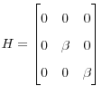
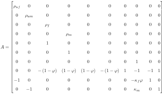
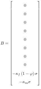
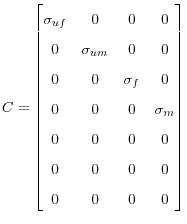
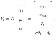
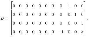
A Structural Matrices for the Economy
Recall that I can represent the structural equations of the economy as

where
 ,
,  ,
,  .
.
 ,
, ,
, .
.
References
Aoki, Kosuke. (2001). "Optimal Monetary Policy Responses to Relative-Price Changes." Journal of Monetary Economics 48, 55-80.Ball, L. and D. Romer. (1990). "Real Rigidities and the Non-Neutrality of Money." Review of Economic Studies 57, 183-203.
Barro, Robert J. and David B. Gordon. (1983). "A Positive Theory of Monetary Policy in a Natural Rate Model." Journal of Political Economy 91, 589-610.
Basu, Susanto. (1995). "Intermediate Goods and Business Cycles: Implications for Productivity and Welfare." American Economic Review 85, 512-531.
Batini, Nicoletta and Anthony Yates. (2003). "Hybrid Inflation and Price-Level Targeting." Journal of Money, Credit, and Banking 35, 283-300.
Benigno, Pierpaolo and Michael Woodford. (2003). "Optimal Monetary and Fiscal Policy: A Linear-Quadratic Approach." NBER Macroeconomics Annual, 271-333.
Berg, Claes and Lars Jonung. (1999). "Pioneering Price Level Targeting: The Swedish Experience 1931-1937." Journal of Monetary Economics 43, 525-551.
Bernanke, Ben S., Thomas Laubach, Frederic S. Mishkin, and Adam S. Posen. (1999). Inflation Targeting. Princeton, NJ: Princeton University Press.
Bils, Mark and Peter J. Klenow. (2004). "Some Evidence on the Importance of Sticky Prices." Journal of Political Economy 112, 947-985.
Blanchard, Olivier J. (1983). "Price Asynchronization and Price Level Inertia." In Inflation, Debt, and Indexation, edited by R. Dornbusch and M. H. Simonsen, pp. 3-24. Cambridge, MA: MIT Press.
Blinder, Alan S., Elie R. D. Canetti, David E. Lebow and Jeremy B. Rudd. (1998). Asking About Prices: A New Approach to Understanding Price Stickiness. New York, NY: Russell Sage Foundation.
von Böhm-Bawerk, Eugen. (1884). Capital and Interest. (Reprinted in 1959) South Holland: Libertarian Press.
Bouakez, Hafedh, Emanuela Cardia and Francisco J. Ruge-Murcia. (2005). "The Transmission of Monetary Policy in a Multi-Sector Economy." Working Paper, University of Montreal.
Calvo, Guillermo. (1983). "Staggered Prices in a Utility-Maximizing Framework." Journal of Monetary Economics 12, 383-398.
Carlton, Dennis W. (1986). "The Rigidity of Prices." American Economic Review 76, 637-658.
Clarida, R., J. Galí, and Mark Gertler. (1999). "The Science of Monetary Policy: A New Keynesian Perspective." Journal of Economic Literature 37, 1661-1707.
Cooley, Thomas F. and E. C. Prescott. (1995). "Economic Growth and Business Cycles." In Frontiers of Business Cycle Research, edited by Thomas F. Cooley, pp. 1-38. Princeton, NJ: Princeton University Press.
Dixit, Avinash K. and Joseph E. Stiglitz. (1977). "Monopolistic Competition and Optimum Product Diversity." American Economic Review 67, 297-308.
Dixit, Avinash K. and Luisa Lambertini. (2003). "Interactions of Commitment and Discretion in Monetary and Fiscal Policies." American Economic Review 93, 1522-1542.
Erceg, Christopher J., Dale W. Henderson, and Andrew T. Levin. (2000). "Optimal Monetary Policy with Staggered Wage and Price Contracts." Journal of Monetary Economics 46, 281-313.
Fuhrer, Jeffrey. C. (1997). "The (Un)Importance of Forward-Looking Behavior in Price Specifications." Journal of Money, Credit, and Banking 29, 338-350.
Fuhrer, Jeffrey C. and G. Schuh Moore. (1995). "Inflation Persistence." Quarterly Journal of Economics 110, 127-159.
Galí, Jordi and Mark Gertler. (1999). "Inflation Dynamics: A Structural Econometric Analysis." Journal of Monetary Economics 44, 195-222.
Givens, Gregory E. (2006). "Revisiting the Delegation Problem in a Sticky Price and Wage Economy." Working Paper, Middle Tennessee State University.
Hanes, Christopher. (1996). "Changes in the Cyclical Behavior of Real Wages 1870-1990." Journal of Economic History 56, 837-861.
Hansen, Gary D. (1985). "Indivisible Labor and the Business Cycle." Journal of Monetary Economics 16, 309-327.
Hornstein, Andreas and Jack Praschnik. (1997). "Intermediate Inputs and Sectoral Comovement in the Business Cycle." Journal of Monetary Economics 40, 573-595.
Huang, Kevin X. D. and Zheng Liu. (2005). "Inflation Targeting: What Inflation Rate to Target?" Journal of Monetary Economics 52, 1435-1462.
Jensen, Henrik. (2002). "Targeting Nominal Income Growth or Inflation?" American Economic Review 92, 928-956.
Jorgenson, Dale W., Frank M. Gollop, and Barbara M. Fraumeni. (1987). Productivity and U.S. Economic Growth. United States of America: North-Holland.
Kim, Jinill. (2000). "Constructing and Estimating a Realistic Optimizing Model of Monetary Policy." Journal of Monetary Economics 45, 329-359.
Kimball, Miles S. (1995). "The Quantitative Analytics of the Basic Neomonetarist Model." Journal of Money, Credit, and Banking 27, 1241-1277.
King, Robert G., Charles I. Plosser and Sergio T. Rebelo. (1988). "Production, Growth and Business Cycles I. The Basic Neoclassical Model." Journal of Monetary Economics 21, 195-232.
King, Mervyn. (2005). "What has Inflation Targeting Achieved?" In The Inflation Targeting Debate, edited by Ben S. Bernanke and Michael Woodford, pp. 11-16. Chicago, IL: University of Chicago Press.
Lambertini, Luisa. (2006). "Monetary-Fiscal Interactions with a Conservative Central Bank." Scottish Journal of Political Economy, 53, 90-128.
Long, John B. and Charles I. Plosser. (1983). "Real Business Cycles." Journal of Political Economy 91, 39-69.
Mankiw, N. Gregory and Ricardo Reis. (2003). "What Measure of Inflation Should a Central Bank Target?" Journal of the European Economic Association 1, 1058-1086.
Néssen, Marianne and David Vestin. (2005). "Average Inflation Targeting." Journal of Money, Credit, and Banking 37, 837-863.
Rogoff, Kenneth. (1985). "The Optimal Degree of Commitment to an Intermediate Monetary Target." Quarterly Journal of Economics 100, 1169-1189.
Rogoff, Kenneth. (1987). "Reputational Constraints on Monetary Policy." Carnegie-Rochester Conference Series on Public Policy 26, 141-181.
Rotemberg, Julio J. and Michael Woodford. (1995). "Dynamic General Equilibrium Models with Imperfectly Competitive Product Markets" In Frontiers of Business Cycle Research, edited by Thomas F. Cooley, pp. 243-293. Princeton, NJ: Princeton University Press.
Rudebusch, Glenn D. (2002). "Assessing Nominal Income Rules for Monetary Policy with Model and Data Uncertainty." The Economic Journal 112, 402-432.
Sbordone, Argia M. (2002). "Prices and Unit Labor Costs: A New Test of Price Stickiness." Journal of Monetary Economics 49, 265-292.
Sims, Christopher A. (2005). "Limits to Inflation Targeting." In The Inflation-Targeting Debate, edited by Ben S. Bernanke and Michael Woodford, pp. 283-308. Chicago, IL: University of Chicago Press.
Strum, Brad E. (2008). "Inflation Persistence and Monetary Policy in an Input-Output Economy," Unpublished Paper, Federal Reserve Board.
Svensson, Lars E. O. (1999a). "Price Level Targeting vs. Inflation Targeting." Journal of Money, Credit, and Banking 31, 277-295.
Svensson, Lars E. O. (1999b). "How Should Monetary Policy Be Conducted in an Era of Price Stability?" In New Challenges for Monetary Policy, Federal Reserve Bank of Kansas City.
Svensson, Lars. E. O. and Michael Woodford. (2005). "Implementing Optimal Policy through Inflation-Forecast Targeting." In The Inflation-Targeting Debate, edited by Ben S. Bernanke and Michael Woodford, pp. 19-83. Chicago, IL: University of Chicago Press.
Vestin, David. (2006). "Price-Level Versus Inflation Targeting" Journal of Monetary Economics 53, 1361-1376.
Walsh, Carl E. (2003a). Monetary Theory and Policy. Cambridge, MA: MIT Press.
Walsh, Carl E. (2003b). "Speed Limit Policies: The Output Gap and Optimal Monetary Policies." American Economic Review 93, 265-278.
Woodford, Michael. (1986). "Stationary Sunspot Equilibria, the Case of Small Fluctuations around a Deterministic Steady State." Manuscript, University of Chicago.
Woodford, Michael. (2001). "Fiscal Requirements for Price Stability." Journal of Money, Credit, and Banking 33, 669-728.
Woodford, Michael. (2003). Interest and Prices: Foundations of a Theory of Monetary Policy. Princeton, NJ: Princeton University Press.
Yan, Won Y., Wenwu Cao, Tae-Sang Chung, and John Morris. (2005). Applied Numerical Methods Using MATLAB, Hoboken, NJ: John Wiley and Sons.
![\displaystyle _{t}\left\{ \sum _{s=t}^{\infty}\alpha_{f}^{s-t}Q_{t,s}\left[ P_... ...u_{f}\right) -V_{fs}\left( i\right) \right] y_{fs}^{d}\left( i\right) \right\}](img24.gif) ,
,
