
The Connection Between House Price Appreciation and Property Tax Revenues
JEL Codes: H71, H2, R28, R31
I. Introduction
In the wake of the real estate boom in the first half of this decade, the property tax revenues of local governments soared, growing 50 percent faster from 2001 through 2005 than they did from 1996 through 2000.1 More recently, the downturn in the housing market has generated concern that property tax revenues will slow or decline.2 Although many analysts and commentators have noted the connection between house prices and property tax revenues (e.g. National League of Cities 2007), there is only limited research on the precise nature of the relationship. This paper provides evidence on two aspects of the relationship. First, the paper addresses the question: "when house prices rise, how much do property tax revenues rise?" This can be viewed as assessing the magnitude of the relationship. Second, the paper addresses the question: "when house prices increase, how long does it take for property tax revenues to increase?" This can be viewed as assessing the timing of the relationship.
Understanding how the evolution of house prices influences property tax revenues is important for at least three reasons. First, the tax plays a central role in financing local public goods in the U.S. Property taxes account for around three-fourths of local government tax revenue and a quarter of total local government revenue. They are particularly important for education as they provide approximately 95 percent of tax revenue for independent school districts (Evans, Murray and Schwab 2001). Given the magnitude of the tax and the fact that most local governments must balance their budgets, fluctuations in property tax revenue - driven by changes in property values - would be expected to influence local government spending decisions.
Second, the connection between property tax revenues and real estate values likely influences the ability of the state and local government sector as a whole to weather fiscal crises. During the state fiscal crisis of 2002 - 2004, localities responded to cuts in state education aid by increasing property tax revenues in order to prevent cuts in education budgets (Dye and Reschovsky 2008). Their ability to do so was likely a function of the strong state of the housing market at that time. Localities may not be well positioned to offset reductions in state funding during the current period of slow economic activity given the softening of house values.
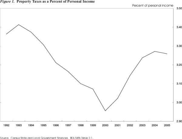
Finally, the relationship between the housing market and property taxes may impact the political viability of the property tax. The share of income devoted to the property tax has risen sharply in recent years (see figure 1), likely due, in part, to the housing boom,3 and this appears to have generated a political backlash. Several states have either enacted, or seriously considered, significant reforms of their property tax in recent years.4
Although past research has examined the effect of home price appreciation on property tax revenues in specific states (e.g. Bloom and Ladd 1982; Cornia and Walter 2006; Dye, McMillen and Merriman 2006; Ladd 1991), I am unaware of any systematic studies conducted on the national level. The lack of previous research may reflect the widely held view that the property tax is a stable revenue source. Indeed, the relative stability of the property tax over the course of the business cycle is often cited as one of the primary virtues of property taxation (e.g. Brunori 2003; Giertz 2006). The recent nationwide housing market run-up and subsequent weakness, however, raises the possibility that the property tax will not be as stable going forward as it has been in the past.
The topic of this paper has parallels with the literature on the marginal propensity to consume (MPC) out of housing wealth (e.g. Carroll, Otuska and Slacalek 2006; Case, Quigley and Shiller 2005; Lehnert 2004; Skinner 1996). This literature seeks to understand how changes in housing market wealth influence personal consumption decisions. Although the literature is far from conclusive, MPC estimates are generally around $0.03 - i.e., every additional dollar of housing wealth leads to an additional 3 cents of consumption. If local public good decisions are viewed through the lens of the median voter model (Black 1948), this paper can be viewed as the public goods analogue to the housing market MPC literature (which examines private goods consumption). When the median voter experiences a wealth shock due to an increase in his home value, he will vote to increase his consumption of public goods by his marginal propensity to consume public goods out of wealth. Although there is a large literature on the marginal propensity to consume public goods out of income - it is generally thought to be equal to around 5 to 10 cents per dollar of income (Hines and Thaler 1995) - I am unaware of any work on the public goods MPC out of wealth. The results of this paper can be interpreted as providing such estimates, subject to a significant caveat: Increases in the value of residential real estate may increase the share of residential property in the tax base relative to commercial and industrial property and thereby increase the median voter's tax price - i.e. the median voter may be required to fund a higher percentage of public expenditures at the margin. The positive price shock may partially offset the positive wealth shock, suggesting that the estimates in this paper should be viewed as lower-bound estimates of the public goods MPC out of housing wealth.
The remainder of the paper is organized as follows. Section II provides background information; Section III presents the empirical estimates of the connection between house prices and property taxes, and Section IV concludes.
II. Background
The property tax is assessed on the value of residential real property (i.e. personal real estate), commercial, business and farm real property, and personal property (e.g. automobiles). Residential real property, the focus of this paper, accounts for approximately 60 percent of taxable assessments and is the largest component of the tax base by a significant margin; commercial, industrial and farm property account for around 30 percent and personal property accounts for less than 10 percent5.
There is significant heterogeneity in the administration of the tax across jurisdictions - a "bewildering array" of different institutional features (Giertz 2006). Abstracting from this heterogeneity, property tax revenue can be defined as being equal to the effective tax rate times the market
value of property
mechanical policy offset
The first question addressed by this paper, "when house prices increase, how much do property tax revenues rise?", can be viewed as estimating the average magnitude of the policy offset. If there is no policy offset, then the elasticity of property tax revenue with respect to house prices will equal 1 - a one percent increase in house prices will generate a one percent increase in property tax revenue - and if there is complete policy offset, the elasticity will equal 0. If there is partial policy offset, the elasticity will range between 0 and 1. Table 1 displays the average annual percent change in property tax revenues, house prices and the effective property tax rate from 2000 to 2005 - a period of rapid house price appreciation. Although property tax revenues grew at a brisk pace over this period, they did not rise as quickly as home values. Policy makers offset some of the mechanical increase by reducing the effective tax rate.
The second question addressed by this paper, "what is the timing of the relationship between house price appreciation and property tax revenue?", is motivated by four institutional features of the property tax likely to generate a delay between changes in the market value of real estate and corresponding changes in property tax revenues. First, the property tax is assessed in an inherently backward looking manner, as the current year's taxes are based on the assessed value of property in the previous year. This feature of the tax suggests that, at a minimum, property tax revenue will respond to house price changes with a lag of at least a year. Second, assessed values often lag market values. In some jurisdictions this occurs by legal mandate. For example, Maryland reassesses once every three years, and increases in the taxable value of property are phased in, in equal increments, over a three year period (Bowman 2006). Third, most states have some form of caps and/or limits on property tax rates, tax revenues or taxable assessments. During periods of rapid house price growth, these limits will prevent assessments or revenues from growing at the same pace as market values. Michigan provides an example; it has an assessment growth limit of the lower of five percent or the rate of inflation (Anderson 2006). When the rate of house appreciation exceeds this limit, assessments will rise at a slower rate than market values and a `stock' of untaxed appreciation will develop. Assessments will catch-up to market values only when house price growth slows below the limit and the `stock' of untaxed appreciation is incorporated into taxable assessments. Finally, the tax is poorly administered in some locales and assessments do not occur in a timely fashion - for example, Utah once went 20 years without conducting meaningful reappraisals. This "poor" administration may be intentional in some jurisdictions, particularly those that elect tax assessors. Such officials may have incentives to delay incorporating changes in market value into assessed values (Cornia and Walters 2006).
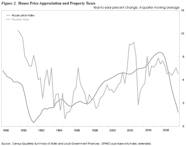
Figure 2 displays the annual growth rate of property tax revenue and house values, as measured by the OFHEO index, from 1988 to 2008.7 The growth rate of both series declined through the early portion of the period. Although house price appreciation reached a trough in mid-1991, property tax revenue growth did not bottom out until the start of 1995, implying that property taxes track real estate prices with a considerable lag. In the more recent period, house price appreciation began falling around the start of 2006, but property taxes have continued to rise at a reasonably strong pace through the end of 2007.
III. Empirics
Two empirical approaches are used in this paper to estimate the relationship between house values and property taxes. The first, referred to as the time-series approach, uses quarterly data aggregated to the national level, and the second, referred to as the micro-data approach, uses annual data on individual governments.
Time-Series
The estimating equation for the time-series approach is:
The ![]() coefficients are the parameters of interest - they measure the elasticity of property tax revenue with respect to house prices. The magnitude of the elasticity, at a point in
time, is determined by the cumulative sum of the
coefficients are the parameters of interest - they measure the elasticity of property tax revenue with respect to house prices. The magnitude of the elasticity, at a point in
time, is determined by the cumulative sum of the ![]() coefficients up to that period. For example, the elasticity four quarters after a change in house prices is equal to the sum of
coefficients up to that period. For example, the elasticity four quarters after a change in house prices is equal to the sum of
![]() and
and ![]() The timing of the relationship
between house prices and property taxes is determined by the evolution of the
The timing of the relationship
between house prices and property taxes is determined by the evolution of the ![]() coefficients over time.
coefficients over time.
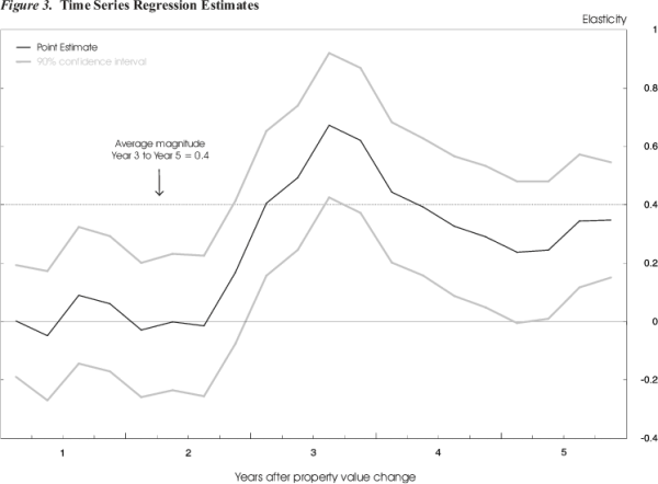
Figure 3 conveys both the magnitude and timing of the connection between house prices and property taxes implied by estimating equation (3). It plots the sum of the ![]() coefficients from the first quarter following a house price change through the 20
coefficients from the first quarter following a house price change through the 20![]() quarter following the change (i.e. the end of the fifth year following the change) and
the associated 90% confidence interval. With regards to timing, a change in house values is estimated to essentially have no effect on property tax revenues in the first two years following the change. The effect of the change in house prices on property taxes then phases in over the course of the
third year and, smoothing through some oscillation in the estimated effect, holds steady in years four and five. The average elasticity in years three through five is 0.4 (the dashed line in the figure) - a 10 percent increase in home values produces a 4 percent rise in property tax revenues. One
can infer from this result that policymakers, on average, choose to offset approximately 60 percent of home value increases by reducing effective tax rates.
quarter following the change (i.e. the end of the fifth year following the change) and
the associated 90% confidence interval. With regards to timing, a change in house values is estimated to essentially have no effect on property tax revenues in the first two years following the change. The effect of the change in house prices on property taxes then phases in over the course of the
third year and, smoothing through some oscillation in the estimated effect, holds steady in years four and five. The average elasticity in years three through five is 0.4 (the dashed line in the figure) - a 10 percent increase in home values produces a 4 percent rise in property tax revenues. One
can infer from this result that policymakers, on average, choose to offset approximately 60 percent of home value increases by reducing effective tax rates.
These estimates must be interpreted with caution. Housing prices incorporate both current and expected future economic conditions. An area which receives a positive economic shock may simultaneously increase demand for local public goods and bid up house prices, both in response to expected
income gains.9 Such a situation would generate a spurious correlation between house prices and property taxes. Although this and other endogeneity concerns may
be mitigated by controlling for changes in income (the ![]() vector in equation (3)) and the more extensive set of control variables employed below, the fact remains that
virtually any unobserved factor that influences housing prices may also alter demand for public goods consumption. Accordingly, the results of this paper should be viewed as establishing the magnitude and timing of the correlation between house price appreciation and property tax revenue, not as
providing strictly causal estimates of the relationship.10 The timing of the relationship between house prices and property taxes does, however, provide some
assurance that the estimated correlation is not purely spurious. An unobserved shock which altered both house values and public goods demand would likely generate a change in property tax revenue relatively quickly. It seems unlikely that a change in public goods demand would take three years to
manifest itself.
vector in equation (3)) and the more extensive set of control variables employed below, the fact remains that
virtually any unobserved factor that influences housing prices may also alter demand for public goods consumption. Accordingly, the results of this paper should be viewed as establishing the magnitude and timing of the correlation between house price appreciation and property tax revenue, not as
providing strictly causal estimates of the relationship.10 The timing of the relationship between house prices and property taxes does, however, provide some
assurance that the estimated correlation is not purely spurious. An unobserved shock which altered both house values and public goods demand would likely generate a change in property tax revenue relatively quickly. It seems unlikely that a change in public goods demand would take three years to
manifest itself.
Table 2 presents additional time-series estimates from a model using annual data, as opposed to quarterly data. Column (1) presents the basic specification. The sum of the coefficients on the change in house prices from years ![]() and
and ![]() is small and imprecise, suggesting that house prices have little impact on property tax revenues in the first two years
following the change in prices. The sum of the coefficients from years
is small and imprecise, suggesting that house prices have little impact on property tax revenues in the first two years
following the change in prices. The sum of the coefficients from years ![]() through
through ![]() ,
however, is equal to 0.44 and can be distinguished from zero. The annual model therefore indicates that it takes 3 years for a change in house prices to influence growth in property tax revenue and that the cumulative elasticity is equal to around 0.4 - conclusions very similar to those produced by
the quarterly model.
,
however, is equal to 0.44 and can be distinguished from zero. The annual model therefore indicates that it takes 3 years for a change in house prices to influence growth in property tax revenue and that the cumulative elasticity is equal to around 0.4 - conclusions very similar to those produced by
the quarterly model.
The estimate becomes more precise when the first two lags of the change in house prices are omitted (column (2)), likely because changes in house prices display a high degree of serial correlation and the resulting multi-collinearity reduces the precision of the individual
estimates. The increased precision makes it feasible to control for additional variables. Column (3) adds the lagged change in property tax revenues to the specification in order to control for persistence in the growth rate of property tax revenue. Column (4)
controls for changes in the stock of residential property. The rate of residential construction tends to be elevated during periods of strong growth in house prices and growth in the housing stock will increase property tax revenues independently of house price increases. It is therefore possible
that the estimated elasticity between house prices and property tax revenues spuriously reflects (or partially reflects) changes in the stock of housing. Changes in both the price and stock of commercial property are also included as controls because they too can influence property tax revenue and
may be correlated with changes in the price of residential real estate. Column (5) controls for changes in the tax bases of the other major state and local government taxes - personal income (personal income tax base), personal consumption (sales tax base), and corporate profits (corporate income
tax base). This is to control for the possibility that state and local governments substitute property tax revenue for other forms of tax revenue during times of fiscal stress (Dye and Reschovsky 2008). None of these control variables substantively alter the results. No attempt is made to control
for property tax caps or limitations. The effectiveness of these limitations is already the subject of a large literature (e.g. Dye and McGuire 1997; Merriman 1987; Fisher and Gade 1991; Preston and Ichniowski 1991). The ![]() estimates capture the average response of policy makers, both those making unconstrained decisions and those making decisions constrained by caps and/or limits.
estimates capture the average response of policy makers, both those making unconstrained decisions and those making decisions constrained by caps and/or limits.![]() 11
11
Micro-Data
The micro-data regressions utilize a panel of data on individual local governments that directly raise property tax revenues. The micro-data provides a much greater range of variation in house prices than the time-series and this allows for testing the hypothesis that local governments respond differently to unusually large house price increases, unusually small house price increases and negative house price changes, relative to typical sized house price increases. For instance, it is possible that governments will offset a greater proportion of very large house price increases because tax increases beyond a certain size are politically unacceptable. A drawback of the micro-data approach is that it must be executed over a shorter time horizon than the time-series estimates (the data permits running the model from 1985 - 2005, compared to 1976 - 2007 for the annual time-series estimates).
The property tax data is drawn from the Census Bureau's State and Local Government Finance Data, and the OFHEO all-transactions index is used to measure housing prices. Both the state-level and the MSA-level version of the OFHEO index are used. Use of the state-level index provides a larger sample (local governments located outside of MSAs can be included in the sample) while use of the MSA-level sample provides a greater range of house price changes. See the Data Appendix for additional information on the data sources.
The micro-data estimation equation is
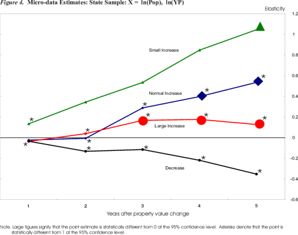
Figure 4 graphically presents the results of estimating equation (4) using the state sample (Appendix Table A1 presents the full coefficient estimates). The vector of control variables, ![]() , includes five lags each of the log of population and the log of personal income, both measured at the state level. In addition to the elasticity estimates, the figure displays the results of two hypothesis tests for each estimate. The first is the standard test for being able to
distinguish the estimate from zero. The null hypothesis is that the elasticity estimate is equal to zero - i.e. that policy makers completely offset changes in house prices. Estimates for which the null hypothesis can be rejected are denoted by large shapes, and estimates for which the null
hypothesis cannot be rejected are denoted by small shapes. The null hypothesis for the second test is that the elasticity estimate is equal to one - i.e. that policy makers engage in no offset and allow the full value of house price changes to pass into property tax revenues. Estimates for which
this second null hypothesis can be rejected are denoted by an asterisk.
, includes five lags each of the log of population and the log of personal income, both measured at the state level. In addition to the elasticity estimates, the figure displays the results of two hypothesis tests for each estimate. The first is the standard test for being able to
distinguish the estimate from zero. The null hypothesis is that the elasticity estimate is equal to zero - i.e. that policy makers completely offset changes in house prices. Estimates for which the null hypothesis can be rejected are denoted by large shapes, and estimates for which the null
hypothesis cannot be rejected are denoted by small shapes. The null hypothesis for the second test is that the elasticity estimate is equal to one - i.e. that policy makers engage in no offset and allow the full value of house price changes to pass into property tax revenues. Estimates for which
this second null hypothesis can be rejected are denoted by an asterisk.
The response of property tax revenue to a normal housing price increase, which corresponds to an increase that falls within the middle two quartiles of positive house price changes (encompassing price changes from 3 to 8 percent), is remarkably similar both in timing and magnitude to the time-series estimates. Property tax revenue does not respond to a change in housing prices until three years after the change and the average elasticity in years three, four and five following the house price change is equal to around 0.4. Both null hypotheses can be rejected for years four and five following the house price change and it is therefore possible to rule out both full offset and no offset.
The elasticity estimates for large house price increases have a similar time profile but are smaller in magnitude, equal to around 0.2. When house prices rise by an unusually large amount, policy makers offset more of the increase than they would for a typical size increase. Policy makers and/or voters may prefer to avoid very large increases in property tax burdens. Alternatively, locations prone to substantial house price increases may be more likely to have property tax limitations in place which prevent large increases in tax bills.
The elasticity estimates for small changes are much larger, equal to around 1 in the fifth year following a change in house prices. These estimates suggest that when house price appreciation is anemic, policy makers offset little to none of the increase. It should be noted that it is generally not possible to statistically distinguish between the "normal increase" elasticity estimates and the "small increase" and the "large increase" elasticity estimates.
The elasticity estimates for house price decreases are negative, indicating that policy makers more than offset the impact of house price declines on property tax revenues. Although the confidence intervals around these estimates are quite large (see Appendix Table A1), it is possible to distinguish them from one - policy makers offset house price depreciation by raising effective tax rates such that tax revenues do not fall by the full amount implied by the decline in house prices.
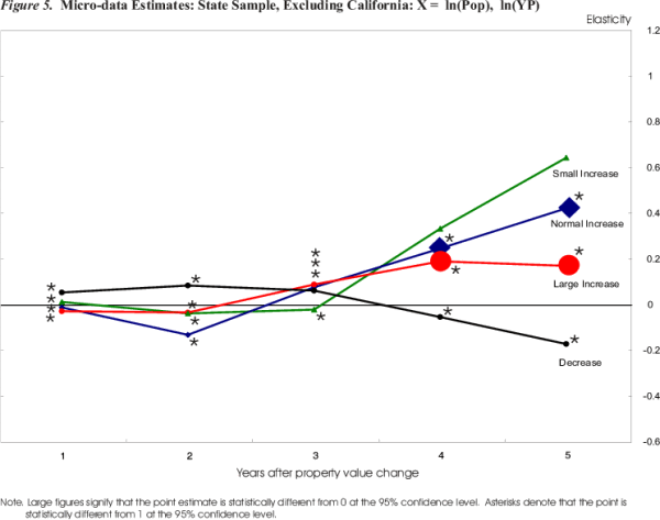
Figure 5 displays state sample estimates which exclude California.13 California has very stringent property tax limitations (Sheffrin 2005) and the
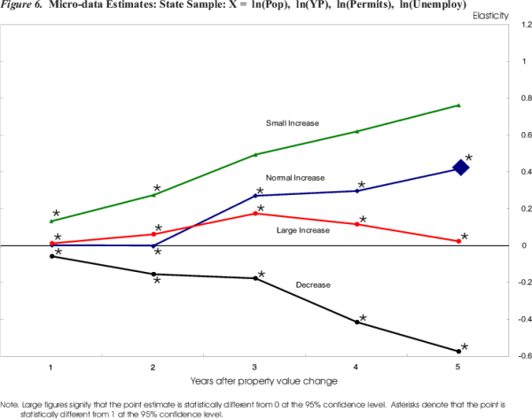
response of property tax revenue to house price changes may differ from the rest of the nation as a result. Figure 6 utilizes the full state sample and adds to the control vector, ![]() , five lags
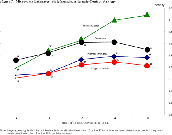
each of the log of total residential building permits issued (to control for increases in the stock of residential property) and the unemployment rate (to control for local economic conditions). Figure 7 displays the results of a different control strategy. The control vector,
, five lags
each of the log of total residential building permits issued (to control for increases in the stock of residential property) and the unemployment rate (to control for local economic conditions). Figure 7 displays the results of a different control strategy. The control vector, ![]() , is replaced by a set of census region-year fixed effects and local government-specific linear trends. The region-year effects control for any time-varying factors, such as economic shocks, at the region
level; the trends control for any factor, such as population growth, which evolves in a gradual, linear manner at the level of the individual locality.14
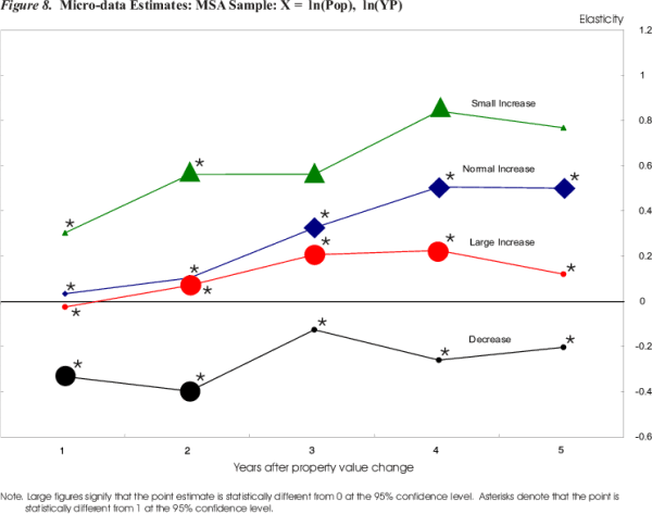
Finally, figure 8 displays the results of estimating the model at the MSA level (with the
, is replaced by a set of census region-year fixed effects and local government-specific linear trends. The region-year effects control for any time-varying factors, such as economic shocks, at the region
level; the trends control for any factor, such as population growth, which evolves in a gradual, linear manner at the level of the individual locality.14
Finally, figure 8 displays the results of estimating the model at the MSA level (with the ![]() vector including the log of population and the log of personal income).
vector including the log of population and the log of personal income).
The "normal increase" elasicities are quite robust to the alternative estimation strategies. The "large increase" and "small increase" estimates are somewhat more variable across the different specification but produce conclusions generally similar to those discussed above. The "decrease" elasticities are also similar to those discussed above, with the exception of figure 7, which employs the region-year and government trend approach. In this instance, the estimates are positive, large in magnitude, and can be distinguished from zero, suggesting that house price depreciation produces large decreases in property tax collections. It is possible that the region-year/trend approach is not as successful as the control variable strategy at controlling for negative economic shocks, which reduce home prices and also reduce demand for public services.
IV. Conclusion
The evidence suggests that property tax revenues are quite responsive to changes in house prices. Although it takes several years for house price appreciation to feed through to property tax revenues, the long-run elasticity is on the order of 0.4. On average, policy makers are estimated to respond to increasing home prices by reducing effective tax rates so as to offset 60 percent of the increase in tax revenue that would have occurred in the absence of a change in the effective tax rate. Institutional features of the property tax, such as delays in bringing assessed values into line with market values and caps and limitations on the tax, likely explain the lag between house prices and tax revenues (and may also influence the magnitude of the relationship.)
There is some evidence that the elasticity is smaller for unusually large house price changes, suggesting that policy makers and voters may prefer to avoid unusually large increases in property tax bills. Similarly, there is evidence that during periods of unusually sluggish house price growth the elasticity is larger, suggesting that policy makers and voters may not want tax revenue growth to slow too much. The evidence on the impact of house price depreciation is somewhat mixed, but on the whole there is little evidence that house price declines influence property tax revenues. It appears that policy makers raise effective tax rates to offset declines in tax revenue arising from downward swings in the housing market. These estimates should be interpreted cautiously because they come from a sample in which most house price declines are relatively small. Thus, the results may not accurately predict the response of local governments to some of the large price declines that have occurred in different parts of the country, given the political difficulty of increasing tax rates under such circumstances.
This paper's estimates reflect the typical behavior of the local government sector as a whole and may not be valid for individual states or communities. For instance, states with stringent property tax limitations, such as California, may have a smaller elasticity of property tax revenue with respect to property values than estimated here. Similarly, states such as Virginia, which have few property tax limitations and bring assessed values into line with market values relatively quickly, may have a shorter lag between real estate appreciation and tax revenues than the estimates in this paper would suggest.
If public good allocation decisions correspond to the median voter model, this paper can be viewed as the public goods equivalent to the literature on the marginal propensity to consume out of housing wealth (which focuses on private goods consumption). Using sample averages, the 0.4 elasticity estimate implies that the marginal propensity to consume local public goods out of housing wealth is equal to 4/10 cent - i.e. each dollar of additional housing wealth increases public goods consumption by $0.004 (see the Data Appendix for details on this calculation). As a reference point, the marginal propensity to consume out of housing wealth for private goods is generally thought to be around $0.03 - a little over seven times as large. As discussed more fully in the introduction, the MPC interpretation is subject to the caveat that this paper's results may reflect both a wealth shock and a partially offsetting price shock. The MPC estimate should therefore be seen as a lower-bound estimate.
Alternatively, if public good allocation decisions correspond more closely to a Leviathan model in which public officials seek to maximize tax revenues (Brennan and Buchanan 1980), the results suggest that public officials find it easier to increase revenues when it does not require a tax rate increase. In fact, the evidence presented here suggests that periods of house price appreciation allow them to increase revenues while simultaneously lowering tax rates.
Acknowledgements
I thank the following individuals for helpful comments and suggestions: Nathan Anderson, Samuel Brown, Jane Dokko, Eric Engen, Glenn Follette, Amanda Kowalski, Andrea Kusko, David Reifschneider, Dan Sichel, Larry Slifman and participants at the Spring 2008 NTA State and Local Symposium. Thanks to Brian McGuire, Daniel Stenberg and particularly Samuel Brown for excellent research assistance. The analysis and conclusions set forth are those of the author and do not indicate concurrence by other members of the Federal Reserve research staff or the Board of Governors.
References
Anderson, Nathan. "Property Tax Limitations: An Interpretative Review." National Tax Journal 59 No. 3 (September, 2006): 685-94.
Bowman, John H. "Property Tax Policy Responses to Rapidly Rising Home Values: District of Columbia, Maryland, and Virginia." National Tax Journal 59 No. 3 (September, 2006): 717-33.
Black, Duncan, "On the Rationale of Group Decision-Making," Journal of Political Economy 56 No. 1 (1948): 23-34.
Bloom, Howard and Helen Ladd. "Property Tax Revaluation and Tax Levy Growth." Journal of Urban Economics 11 No. 1 (January, 1982): 73-84.
Brennan, Geoffrey and James Buchanan. The Power to Tax: Analytical Foundations of a Fiscal Constitution. New York: Cambridge University Press, 1980.
Brunori, David. Local Tax Policy: A Federalist Perspective. Washington D.C.: Urban Institute Press, 2003.
Carroll, Christopher D., Misuzu Otsuka and Jirka Slacalek. "How Large Is the Housing Wealth Effect? A New Approach." Working Paper, 2006.
Case, Karl E., John M. Quigley, and Robert J. Shiller. "Comparing Wealth Effects: The Stock Market versus the Housing Market." Advances in Microeconomics 5 No. 1 (2005): Article 1.
Cornia, Gary and Lawrence Walters. "Full Disclosure: Controlling Property Tax Increases During Periods of Increasing Housing Values." National Tax Journal 59 No. 3 (September, 2006): 735-49.
Dye, Richard and Andrew Reschovsky. "Property Tax Responses to State Aid Cuts in the Recent Fiscal Crisis." Public Budgeting & Finance, Vol. 28, Issue 2, 2008.
Dye, Richard and Therese McGuire. "The Effect of Property Tax Limitation Measures on Local Government Fiscal Behavior." Journal of Public Economics 66 No. 3 (December, 1997): 469-487.
Dye, Richard, Daniel McMillen and David Merriman. "Illinois' Response to Rising Residential Property Values: An Assessment Growth Cap in Cook County." National Tax Journal 59 No. 3 (September, 2006): 707-16.
Evans, William, Sheila Murray and Robert Schwab. "The Property Tax and Education Finance." In Property Taxation and Local Government Finance, edited by Wallace Oates, 209-235. Cambridge, MA: Lincoln Institute of Land Policy, 2001.
Fisher, Ronald and Mary Gade. "Local Property Tax and Expenditure Limits." In State and Local Finance for the 1990s: A Case Study of Arizona, edited by Therese McGuire and Dana Naimark, 449-464. Tempe, AZ: Arizona State University, 1991.
Giertz, J. Fred. "The Property Tax Bound." National Tax Journal 59 No. 3 (September, 2006): 695-705.
Hines, James R., Richard H. Thaler. "Anomalies: The Flypaper Effect." Journal of Economic
Perspectives 9 No. 4 (Fall, 1995): 217-26.
Ladd, Helen. "Property Tax Revaluation and Tax Levy Growth Revisited." Journal of Urban Economics 30 No. 1 (July, 1991): 83-99.
Lehnert, Andreas. "Housing, Consumption, and Credit Constraints." FEDS Working Paper No. 2004-63. Washington D.C.: Federal Reserve Board, 2004.
Merrick, Amy. "Property Tax Frustration Builds: States, Cities Revise Strategy as Homeowners Protest Rising Levies." The Wall Street Journal (December 18, 2007).
Merriman, David. The Control of Municipal Budgets: Toward the Effective Design of Tax and Expenditure Limitations. Westport, CT: Greenwood Press, 1987.
National League of Cities. City Fiscal Conditions 2007. Washington, D.C.: October, 2007.
Preston, Anne and Casey Ichniowski. "A National Perspective on the Nature and Effects of the Local Property Tax Revolt, 1976-1986." National Tax Journal 44 No. 2 (June, 1991): 123-145.
Sheffrin, Steven. "Proposition 13/Property Tax Caps." In The Encyclopedia of Taxation and Tax Policy, edited by Joseph Cordes, Robert Ebel and Jane Gravelle, 321-323. Washington, D.C.: Urban Institute Press, 2005.
Skinner, J. S. "Is Housing Wealth a Sideshow?" In Advances in the Economics of Aging, National Bureau of Economic Research Report, 241-268. Chicago: 1996.
Table 1: Annual Percent Changes in Property Tax Revenues, House Prices, and Property Tax Rebate
| Variable | 2000 - 2005
Average |
| 1) House Prices | 7.9% |
| 2) Effective Property Tax Rate | -1.7% |
| 3) Property Tax Revenues | 6.1% |
Source: OFHEO purchase-only index. BEA NIPA Table 3.3, line 9. Author's calculations. The effective property tax rate, row 2, is defined as (0.6*property tax revenue)/(house prices), where 0.6 reflects the fact that approximately 60% of total property tax revenues come from residential real estate.
Table 2: Annual Time Series Regressions
Dependent Variable: ![]() log(Property Tax Revenue)
log(Property Tax Revenue)
| #1 | #2 | #3 | #4 | #5 | |
| 1) Constant | 0.038** | 0.037** | 0.027** | -0.046** | 0.015 |
| Constant (Standard Error) | (0.008) | (0.007) | (0.008) | (0.012) | (0.017) |
| 2) |
-0.066 | ||||
| (0.206) | |||||
| 3) |
0.085 | ||||
| (0.269) | |||||
| 4) |
0.422** | 0.462** | 0.382** | 0.480** | 0.418** |
| (0.193) | (0.107) | (0.107) | (0.199) | (0.142) | |
| 5) |
0.242** | ||||
| (0.114) | |||||
| Controls for: Stock of Residential and Commercial Property, Price of Commercial Property | X | ||||
| Controls for: Personal Income Tax Base, Corporate Income Tax Base, Sales Tax Base | X | ||||
| Observations | 29 | 29 | 29 | 28 | 29 |
| Degrees of Freedom | 25 | 27 | 26 | 19 | 15 |
| R-Square | 0.413 | 0.410 | 0.498 | 0.679 | 0.711 |
| Adj. R-Square | 0.342 | 0.388 | 0.459 | 0.545 | 0.460 |
Note: Property Tax Revenue is the BEA state and local property tax revenue series. House Price Index is the OFHEO price index for owner-occupied real estate, purchases only extended. Column #4 controls for the contemporaneous
and lag![]() of the log change in the following variables: BEA net stock of private residential structures and BEA net stock of private non-residential structures. It also controls for lags t-1, t-2, and
of the log change in the following variables: BEA net stock of private residential structures and BEA net stock of private non-residential structures. It also controls for lags t-1, t-2, and ![]() of the log change in the NREI price index for commercial real estate. Column #5 controls for the contemporaneous and lags
of the log change in the NREI price index for commercial real estate. Column #5 controls for the contemporaneous and lags ![]() and
and ![]() of the log change in the following variables: BEA personal income, BEA corporate profits before tax, and BEA personal consumption expenditures.
of the log change in the following variables: BEA personal income, BEA corporate profits before tax, and BEA personal consumption expenditures.
* Value significant at 10%
** Value significant at 5%
Appendix Table A1:
Micro-Data Estimates: State Sample: X = ![]() ln(Pop),
ln(Pop), ![]() ln(YP)
ln(YP)
| Change in House Price | Cumulative Point Estimate | Upper 95% CI | Lower 95% CI |
| Normal Increase, Year 1 |
-0.023 | 0.073 | -0.119 |
| Normal Increase, Year 2 |
-0.005 | 0.233 | -0.244 |
| Normal Increase, Year 3 |
0.289 | 0.652 | -0.075 |
| Normal Increase, Year 4 |
0.399 | 0.665 | 0.132 |
| Normal Increase, Year 5 |
0.536 | 0.801 | 0.271 |
| Large Increase, Year 1 |
-0.035 | 0.017 | -0.088 |
| Large Increase, Year 2 |
0.040 | 0.172 | -0.093 |
| Large Increase, Year 3 |
0.169 | 0.327 | 0.011 |
| Large Increase, Year 4 |
0.177 | 0.280 | 0.075 |
| Large Increase, Year 5 |
0.128 | 0.278 | -0.022 |
| Small Increase, Year 1 |
0.135 | 0.527 | -0.257 |
| Small Increase, Year 2 |
0.346 | 1.127 | -0.436 |
| Small Increase, Year 3 |
0.536 | 1.596 | -0.524 |
| Small Increase, Year 4 |
0.849 | 1.942 | -0.245 |
| Small Increase, Year 5 |
1.046 | 1.990 | 0.103 |
| Decrease, Year 1 |
-0.034 | 0.234 | -0.301 |
| Decrease, Year 2 |
-0.131 | 0.309 | -0.571 |
| Decrease, Year 3 |
-0.114 | 0.245 | -0.474 |
| Decrease, Year 4 |
-0.218 | 0.186 | -0.623 |
| Decrease, Year 5 |
-0.352 | 0.171 | -0.875 |
Note: Cumulative point estimates for normal house price increases are the sum of the ![]() coefficients from the first
year following the house price change through year
coefficients from the first
year following the house price change through year ![]() . For example, the cumulative point estimate for the second year following a normal house price increase is
. For example, the cumulative point estimate for the second year following a normal house price increase is
![]() . Cumulative point estimates for other changes in house prices are the sum of the
. Cumulative point estimates for other changes in house prices are the sum of the ![]() coefficients for the normal increase and the sum of the
coefficients for the normal increase and the sum of the ![]() coefficients for the other changes in house prices. For example, the point estimate for the second year following a small house price increase is
coefficients for the other changes in house prices. For example, the point estimate for the second year following a small house price increase is
![]() ,
,
![]() ,
,![]() .
.
Data Appendix
Time-Series Regressions (equation (3); figure 3 and table 2)
Data for property tax revenues comes from the Bureau of Economic Analysis (BEA) National Income and Product Accounts (NIPA) Table 3.3, line 9. Data for house prices is an extended version of the purchase-only index from the Office of Federal Housing Enterprise Oversight (OFHEO). The purchase-only index starts in the first quarter of 1991; all values from 1975 through 1990 are from OFHEO's all-transactions index, normalized to equal 100 in 1991 Q1. Personal income comes from BEA NIPA Table 2.1, line 1. For the annual models displayed on Table 2, annual levels of the variables are set equal to the fourth quarter value for the year. The log change of the variables can therefore be interpreted as a year-to-year percent change. The net stock of private residential structures and net stock of private non-residential structures come from BEA Fixed Assets Table 2.1, line 59 and Table 1.1, line 6, respectively. Data for commercial real estate prices is the weighted average of the office, warehouse, and retail transaction price indices from the National Real Estate Investor (NREI). Corporate profits (BEA NIPA Table 1.14, line 32) are before taxes and exclude inventory valuation adjustment (IVA) and capital consumption adjustments (CCAdj). Personal consumption expenditures are from BEA NIPA Table 1.1.5, line 2.
Panel Regressions(equation (4);figures 4 - 8)
Government units that had missing or zero values for property tax revenues were excluded from the sample. Government units with annual changes in property tax revenues exceeding 100% were dropped from the sample - such changes likely arise from unusual events, such as the consolidation of localities, unrelated to the connection between house prices and property tax revenues. For variables available quarterly, annual values were set according to the fiscal year ending variable provided in the Annual Survey of Governments (ASG) data - i.e. if the fiscal year ended in the second quarter, then we used the second quarter data point (or the last month in the quarter) as the value for the year. If the fiscal year ending date was missing, we assumed the fiscal year ended on June 30, the most common fiscal year end. The log change of the variables can therefore be interpreted as a fiscal year-to-fiscal year percent change. The MSA-level regressions, depicted in figure 8, use the MSA boundaries established by OMB Bulletin No. 08-01 (November 20, 2007) and group individual units in MSAs using the Federal Information Processing Standard (FIPS) codes provided in the ASG individual data files. This eliminated government entities outside of MSAs. We utilized the MSA-level house prices (OFHEO--all-transaction index), personal income (BEA--Local Area Personal Income, CA1-3, 1.0), and population (BEA--Local Area Personal Income, CA1-3, 2.0). Sample sizes for the state panel regressions (figures 4 - 7) are on the order of 250,000 observations. The sample size for the MSA panel regression (figure 8) is approximately 140,000 observations.
Public goods MPC out of housing wealth calculation
The marginal propensity to spend on public goods out of housing wealth is calculated as follows.
 and
and
![]() therefore
therefore
![]()
For this calculation, ![]() is aggregate property tax revenue from single family residential real estate and
is aggregate property tax revenue from single family residential real estate and ![]() is the aggregate value of single family residential real estate. The elasticity is assumed to be 0.4 based on the evidence presented in Section III. R = ($376 billion * 0.5); the $376 billion is total aggregate property tax revenue based on the Census Bureau's 2006 Quarterly
Summary of State and Local Government Tax Revenues and the 0.5 represents the percent of total property tax payments accounted for by single family homes (author's calculation from the 1987 and 1991 Census of Governments). V = $18,559 billion; the value of owner-occupied, single
family property in the 2006 American Community Survey.
is the aggregate value of single family residential real estate. The elasticity is assumed to be 0.4 based on the evidence presented in Section III. R = ($376 billion * 0.5); the $376 billion is total aggregate property tax revenue based on the Census Bureau's 2006 Quarterly
Summary of State and Local Government Tax Revenues and the 0.5 represents the percent of total property tax payments accounted for by single family homes (author's calculation from the 1987 and 1991 Census of Governments). V = $18,559 billion; the value of owner-occupied, single
family property in the 2006 American Community Survey.
Footnotes
*The views expressed are those of the author and do not necessarily represent those of the Board of Governors or other members of its staff. Return to Text