
Firms' Relative Sensitivity to Aggregate Shocks and the Dynamics of Gross Job Flows
Keywords: Aggregate shocks, gross job flows, firm heterogeneity
Abstract:
JEL Classification: E24, E32, J23
1 Introduction
Job reallocation is a significant and cyclically sensitive activity. The literature has identified substantial heterogeneities across firm classes and economic sectors in terms of the magnitude and the volatility of job creation and job destruction. In this paper, after confirming some of these heterogeneities, we analyze how the importance of aggregate shocks for fluctuations in gross job flows differs across firm size and age and how these differences affect the dynamics of aggregate job flows.
Using the Longitudinal Research Database (LRD) data for the U.S. manufacturing sector, Davis and Haltiwanger (1990, 1992) and Davis et al. (1996) find that job reallocation is countercyclical mostly because of large and old plants, as job destruction for these plants is substantially more volatile than job creation.1Burgess et. al. (2000) emphasize the firm's lifecycle and conclude that young and dying firms account for about a third of all job reallocation. The countercyclical nature of job reallocation is later questioned by Boeri (1996) as it seemed to be specific to manufacturing and result from a selection bias against small and young firms in the LRD data. Foote (1998) confirms this with Michigan unemployment insurance data, where the higher volatility of job destruction with respect to the volatility of job creation in manufacturing does not hold in other sectors like services and retail trade. Foote then argues that the cyclical properties of input reallocation are a function of the sector's trend growth rate. In analyzing the importance of composition effects for some of these facts, Davis and Haltiwanger (1999) conclude that, among four-digit manufacturing sectors, the relative volatility of job destruction is positively affected by firm size and age after controlling for trend growth. This suggests that the higher relative volatility of job destruction in manufacturing partly results from the predominance of large and old firms in this sector, with the opposite occurring in services.
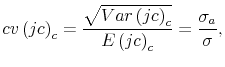
In this paper, we provide further evidence on how different firm size and age classes influence the cyclical properties of aggregate job reallocation. We begin by presenting firm-level job flows statistics for the Portuguese economy and four economic sectors, and later tabulate job flows by firm size and age. Our findings are consistent with those in other international studies. Previous studies for Portugal, such as Blanchard and Portugal (2001) , only contained information for the overall economy and the manufacturing sector and did not include an analysis of heterogeneities by firm size and age. Based on a simple model of job flows dynamics, with both aggregate and idiosyncratic shocks, we propose the coefficient of variation of gross job flows as a proxy for the importance of aggregate shocks for fluctuations in job flows at the firm level. Since the coefficient of variation is a scale-independent index of volatility, we interpret this proxy as a measure of firms' relative sensitivity to aggregate shocks. In our data, for both the overall economy and the four economic sectors, we find that large and old firms are more relatively affected by aggregate shocks than small and young firms. Therefore, large and old firms influence more the dynamics of aggregate job flows than the average size of these flows.
Given the markedly heterogeneous job reallocation patterns across firm size and age classes, we then analyze how the higher relative sensitivity to aggregate shocks of large and old firms affects the dynamics of aggregate job reallocation. In the overall economy, the higher sensitivity of large and old firms makes aggregate job reallocation less procyclical than if firm size and age classes were equally sensitive to aggregate shocks, as these firms have lower net job creation rates and less procyclical, or even countercyclical, job reallocation. A similar result applies in the manufacturing and the transportation and public utilities sectors, for both large and old firms, and in the services sector, for old firms. For the other cases, the above result does not apply because of more similar reallocation activity across firm classes. In particular, large firms make aggregate job reallocation in retail trade and services slightly more procyclical than if size classes were equally sensitive to aggregate shocks, as large firms exhibit even more procyclical reallocation than small firms. We conclude that the dynamics of aggregate job reallocation depends disproportionately on the cyclical behavior of large and old firms. Therefore, a relatively higher emphasis should be given to large and old firms when characterizing the business cycle.
The conclusions of the paper appear also important for the literature that analyzes differences in the response to aggregate shocks across firm size and age. Similarly to Li and Weinberg (2003) and Campbell and Fisher (2004) , we use a framework where firms face idiosyncratic and aggregate shocks. However, instead of focusing on the absolute response of adjustment rates to aggregate shocks, which tends to be higher for small and young firms, we analyze the absolute response relative to the average adjustment rate, which also tends to be higher for these firms as they are more exposed to idiosyncratic shocks. That is, we emphasize coefficients of variation instead of standard deviations. Since small and young firms are characterized by higher average rates of adjustment, the absolute volatility of gross job flows should also be higher due to the scale dependence of standard deviations. On the contrary, coefficients of variation are scale independent and show that large and old firms are relatively more affected by aggregate shocks.
The paper is organized as follows. In section 2, we present gross job flows statistics for the Portuguese economy and four one-digit sectors. In section 3, we propose a measure for firms' relative sensitivity to aggregate shocks. In section 4, we analyze heterogeneities across firm size and age classes and how the higher sensitivity to aggregate shocks of large and old firms affects the dynamics of aggregate job reallocation. We conclude in section 5. Three appendices contain a description of the database and the methods we use to obtain gross job flows, an outline of the model simulations and proofs in section 3, and additional details on the decompositions in section 4.
2 Gross Job Flows in the Portuguese Economy
In this section, we present evidence on the dynamics of gross job flows in the Portuguese economy. We use Quadros de Pessoal (QP), a longitudinal employer-employee matched database, with annual data covering the period 1985-2000.2 As background, we present a summary of some macroeconomic developments in the Portuguese economy during this period.
From the mid-1980s to the late-1990s, Portugal went through a process of modernization in infrastructure and market regulations. After joining the European Union (EU) in 1986, Portugal benefited from large amounts of European Structural Funds to promote investment in infrastructure. Until the mid-1990s, Portugal also adopted reforms to enhance competition and liberalize financial markets, a key step in the creation of an economic union in Europe. In addition, from the late-1980s to the early-1990s there was a wave of privatizations of public utilities. As a result of these structural reforms, and the increased liberalization of trade in the EU during this period, some traditional manufacturing sectors, such as textiles, suffered hard, while new opportunities emerged, especially in the retail trade and services sectors.
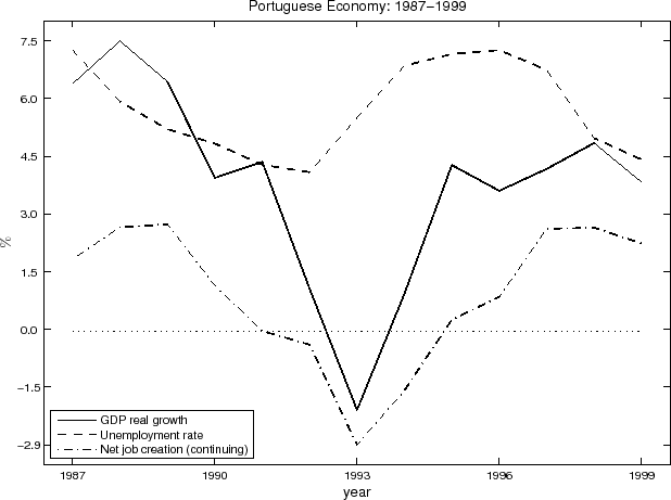
To summarize the business cycle in the period under analysis, figure 2 plots the annual real growth rate of GDP, the unemployment rate, and the net job creation rate among continuing firms.3 The late-1980s was a period of high growth with a declining unemployment rate. This expansion was followed by a downturn in economic activity that hit the bottom in 1993. The ensuing upturn was mild and net job creation reacted only slowly to the improving economy. It is apparent from figure 2 that net job creation has a high positive correlation with growth of real GDP, and that the unemployment rate is countercyclical.
We present in table 1 the evolution of gross job flows for the overall economy during the period under analysis.4 The values for gross job flows are comparable to other international evidence, such as Davis et al. (1996) and Baldwin et al. (1998) . Both the rates of job creation and job destruction and the contribution of births and deaths to gross flows are large. Most job reallocation consists of excess reallocation, with net job creation accounting for only a small fraction. Job creation and job destruction vary procyclically and countercyclically with the business cycle, respectively, and in a way consistent with figure 2.
In table 2, we present some statistics of job flows for the overall economy and four one-digit sectors: manufacturing, services, retail trade, and transportation and public utilities.5 In general, there is considerable reallocation activity and significant cross-sector differences in the magnitude and cyclical behavior of job flows. Consistent with Foote (1998) , sectors with higher net job creation (services and retail trade) exhibit more procyclical reallocation. However, for the overall economy, the average net job growth rate is notably positive while reallocation is only marginally procyclical. As we show in section 4, this result can be partially explained by the behavior of large and old firms.6 Table 2 also reveals the structural changes that occurred in the Portuguese economy during this period. In particular, manufacturing and transportation and public utilities industries suffered large drops in employment share, whereas services and retail trade industries registered steep gains. This is then reflected in the much higher net job creation rates in the last two sectors.
3 Gross Flows and Sensitivity to Aggregate Shocks
In this section, we propose a measure of firms' relative sensitivity to aggregate shocks using a simple model of job flows dynamics. Although the model is mostly descriptive and not entirely built from microfoundations, it allows a clear motivation for the empirical analysis in section 4. Similarly to Bertola and Caballero (1990) , in the study of durable goods consumption, and Foote (1998) , in the analysis of the cyclical volatility of gross job flows, we use a simple model of
![]() adjustment with aggregate shocks.
adjustment with aggregate shocks.
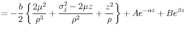
In this model of employment adjustment, firms face proportional adjustment costs and are subject to both idiosyncratic and aggregate shocks. In particular, in the absence of adjustment costs, the firm's optimal employment is determined by,
where
The model assumes that firms choose employment in order to minimize the costs of deviating from frictionless employment, simply modelled as
![]() , net of proportional adjustment costs, given by
, net of proportional adjustment costs, given by
![]() , with future net costs discounted at a rate
, with future net costs discounted at a rate ![]() . Although firms
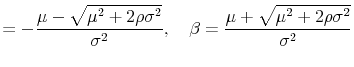
would continuously react to incoming shocks, if adjustment was costless, the non-differentiable adjustment costs imply that firms adjust employment only intermittently. The optimal employment policy is then characterized by two trigger points,
. Although firms
would continuously react to incoming shocks, if adjustment was costless, the non-differentiable adjustment costs imply that firms adjust employment only intermittently. The optimal employment policy is then characterized by two trigger points, ![]() and
and ![]() , defined over the employment gap,
, defined over the employment gap,
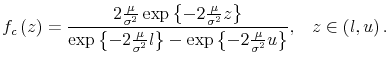
![]() . These trigger points define the maximum deviations allowed before adjustment occurs. With the trigger points and the stochastic properties of the shocks it is possible to
derive an ergodic distribution for each firm's employment gap. While this micro-level distribution is time-invariant, the cross-sectional distribution of firms over the employment gap varies over time. In fact, aggregate shocks cause all firms to move similarly in the gap space, resulting in a
parallel shift of the cross-sectional distribution.
. These trigger points define the maximum deviations allowed before adjustment occurs. With the trigger points and the stochastic properties of the shocks it is possible to
derive an ergodic distribution for each firm's employment gap. While this micro-level distribution is time-invariant, the cross-sectional distribution of firms over the employment gap varies over time. In fact, aggregate shocks cause all firms to move similarly in the gap space, resulting in a
parallel shift of the cross-sectional distribution.
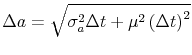
In appendix B, we show that, when the ergodic distribution is used as an approximation for the cross-sectional distribution, the coefficients of variation of gross job creation (jc) and job destruction (jd) can be
simply expressed as the ratio of the standard deviation of the aggregate shock,
![]() , over the standard deviation of employment shocks,
, over the standard deviation of employment shocks, ![]() , which is a
composite of aggregate and idiosyncratic shocks,
, which is a
composite of aggregate and idiosyncratic shocks,
Intuitively, the coefficient of variation of gross job flows can be interpreted as a measure of the relative importance of aggregate shocks for fluctuations in gross job flows at the firm level. Therefore, we call this ratio the firms' relative sensitivity to aggregate shocks.
Since the time-series variation in gross job flows is due in part to changes in the cross-sectional distribution, the above result does not hold exactly when we use this time-varying distribution. However, we show by numerical simulation that the cross-sectional distribution preserves the
positive relation between the ratio
![]() and the coefficients of variation of gross job flows.7
and the coefficients of variation of gross job flows.7
We calibrate the model to match the time-series means and standard deviations of job creation and destruction among continuing firms in the overall economy. The parameter values are the following: an annual discount rate of ![]() ,
, ![]() ; an annual trend growth rate of employment of
; an annual trend growth rate of employment of ![]() ,
,
![]() ; an annual standard deviation of employment shocks of 21.4 percentage
points,
; an annual standard deviation of employment shocks of 21.4 percentage
points,
![]() ; an annual standard deviation of aggregate employment shocks of 1.1
percentage points,
; an annual standard deviation of aggregate employment shocks of 1.1
percentage points,
![]() ; an annual cost of adjustment equal to 3.3 times the annual cost
of deviating from optimal employment, for an adjustment and deviation equal to the average job creation and destruction rates,
; an annual cost of adjustment equal to 3.3 times the annual cost
of deviating from optimal employment, for an adjustment and deviation equal to the average job creation and destruction rates,
![]() .8 The implied
trigger points are
.8 The implied
trigger points are ![]() and
and ![]() . Therefore, the firm only decides to hire
after employment falls below its target by
. Therefore, the firm only decides to hire
after employment falls below its target by ![]() and only decides to fire when employment rises above its target by
and only decides to fire when employment rises above its target by ![]() . Associated with this policy, the time-series average rates of job creation and destruction are
. Associated with this policy, the time-series average rates of job creation and destruction are ![]() and
and ![]() , respectively, the coefficients of variation are 0.14, and the ratio of standard deviations is
, respectively, the coefficients of variation are 0.14, and the ratio of standard deviations is ![]() .9
.9
With this calibration in hand, we vary ![]() around its reference value and analyze the relation between the coefficients of variation of job creation and destruction and the ratio
around its reference value and analyze the relation between the coefficients of variation of job creation and destruction and the ratio
![]() (keeping
(keeping
![]() fixed). In figure 1, we can see that the coefficients of variation obtained from the simulated ergodic distribution satisfy very closely the relationship
presented in (2). We can also see that the dynamics of the cross-sectional distribution accounts for a sizable fraction of the cyclical variation of gross job flows. Notwithstanding this, the coefficients of variation based on the cross-sectional distribution preserve the
positive dependence on the ratio
fixed). In figure 1, we can see that the coefficients of variation obtained from the simulated ergodic distribution satisfy very closely the relationship
presented in (2). We can also see that the dynamics of the cross-sectional distribution accounts for a sizable fraction of the cyclical variation of gross job flows. Notwithstanding this, the coefficients of variation based on the cross-sectional distribution preserve the
positive dependence on the ratio
![]() . Indeed, in the cross-sectional distribution case, the relation appears to be linear, with the coefficients of variation being proportional to the ratio
. Indeed, in the cross-sectional distribution case, the relation appears to be linear, with the coefficients of variation being proportional to the ratio
![]() . Therefore, our interpretation for the coefficients of variation of gross job flows based on equation (2), as a measure of firms' relative sensitivity to
aggregate shocks, remains valid even if we account for the impact of aggregate shocks on the cross-sectional distribution.
. Therefore, our interpretation for the coefficients of variation of gross job flows based on equation (2), as a measure of firms' relative sensitivity to
aggregate shocks, remains valid even if we account for the impact of aggregate shocks on the cross-sectional distribution.
The sensitivity to aggregate shocks is particularly interesting for comparing different classes of firms, as the literature has not directly analyzed potential heterogeneities in this dimension of gross job flows. In the next section, we analyze how heterogeneous are firm size and age classes along this dimension and the implications of these heterogeneities for the dynamics of aggregate job reallocation.
4 Sensitivity to Aggregate Shocks by Size and Age
In this section, we first describe how the importance of aggregate shocks for fluctuations in gross job flows varies by firm size and age, and then we analyze the influence of these firm heterogeneities on the dynamics of aggregate job reallocation.
In order to adopt relative and sector-specific definitions of small versus large and young versus old firms, we partition the set of all firms in two classes, in such a way that each class contains approximately ![]() of total employment.10 Due to the higher prevalence of entry and exit among small and young firms, we restrict our
attention to job flows for continuing firms.11
of total employment.10 Due to the higher prevalence of entry and exit among small and young firms, we restrict our
attention to job flows for continuing firms.11
Tables 3 and 4 contain statistics for size and age classes, respectively. From the size and age cutoffs between classes, we conclude that the size and age distributions are quite different across the four sectors, likely reflecting technological and institutional factors. In particular, the transportation and public utilities and the manufacturing sectors tend to be more populated by large and old firms, whereas the retail trade and the services sectors exhibit a high concentration of small and young firms. We also observe considerable heterogeneities across size and age classes. Small and young firms have high gross job creation and job destruction rates, accounting for a greater share of job reallocation than suggested by their employment share. Moreover, small and young firms exhibit higher net job growth, and, in line with Foote (1998) , reallocation tends to be more procyclical for these firms.
More importantly, small and young firms have lower coefficients of variation of gross job flows. This suggests that fluctuations in job reallocation at the firm level are less determined by aggregate shocks in the case of small and young firms than in the case of large and old firms. As a result, we expect large and old firms to influence proportionately more the cyclical variation of aggregate job flows than the average size of these flows. These inferences appear consistent with a theory of learning and growth, where firms go through an intensive learning process after entry and adjust according to performance, a process that makes idiosyncratic shocks more determinant for employment adjustments of small and young firms (Li and Weinberg, 2003; Campbell and Fisher, 2004) .
We now analyze how the higher relative sensitivity to aggregate shocks of large and old firms affects aggregate job reallocation. The cyclical properties of job reallocation are usually summarized by the coefficient of correlation between the rates of job reallocation and net job creation,
![]() .12 The following
expression for this coefficient suggests that we can also use the ratio of variances as a proxy for the cyclical behavior of job reallocation,13
.12 The following
expression for this coefficient suggests that we can also use the ratio of variances as a proxy for the cyclical behavior of job reallocation,13
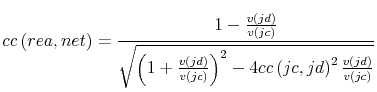 ,
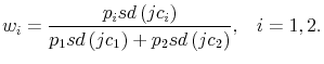
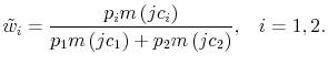
,where we consider the definitions
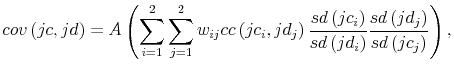
For the case of two firm classes, where ![]() represents the employment share of class
represents the employment share of class ![]() , we consider the following decomposition of the variance of job destruction
, we consider the following decomposition of the variance of job destruction
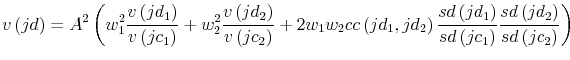 ,
,where
In tables 3 and 4, the adjusted correlations are signaled with
![]() in the last three columns. In the overall economy, the higher net job creation rates and lower sensitivity to aggregate shocks of small and young firms implies that,
after adjustment, the correlation
in the last three columns. In the overall economy, the higher net job creation rates and lower sensitivity to aggregate shocks of small and young firms implies that,
after adjustment, the correlation
![]() becomes higher and the correlations
becomes higher and the correlations
![]() and
and
![]() become higher for small and young firms and lower for large and old firms. Therefore, the higher relative sensitivity of large and old firms makes aggregate
job reallocation less procyclical than if size and age classes were equally sensitive to aggregate shocks and increases the importance of these firms for the dynamics of aggregate gross job flows.
become higher for small and young firms and lower for large and old firms. Therefore, the higher relative sensitivity of large and old firms makes aggregate
job reallocation less procyclical than if size and age classes were equally sensitive to aggregate shocks and increases the importance of these firms for the dynamics of aggregate gross job flows.
In comparison to the other sectors, manufacturing displays small differences in the sensitivity to aggregate shocks between the two firm size and age classes. However, reallocation patterns are strikingly opposite between the two classes: small and young firms exhibit positive net job creation and procyclical reallocation, while large and old firms exhibit negative growth and countercyclical reallocation. Thus, the adjusted correlations imply conclusions similar to the overall economy case: large and old firms influence the dynamics of aggregate job flows more than proportionately to their influence over the average size of these flows and lead job reallocation in manufacturing to be countercyclical.
The evidence for the transportation and public utilities sector is qualitatively similar to that for the manufacturing sector. However, the contrast between the two firm size and age classes is sharper than in manufacturing, as transportation and public utilities industries are mostly composed of large and old firms, with much higher sensitivities to aggregate shocks than small and young firms.15 Consequently, the differences between the adjusted and unadjusted correlations are even higher than in manufacturing, with large and old firms determining the markedly countercyclical behavior of job reallocation in the sector.
Similarly to the other sectors, large and old firms in services and retail trade are more sensitive to aggregate shocks than small and young firms and have a disproportional influence over the dynamics of gross job flows. However, contrary to the other sectors, the reallocation patterns in services and retail trade are, for the most part, quite similar between the two size and age classes. In particular, young and old firms in retail trade show nearly no differences in reallocation activity and the cyclical properties of aggregate reallocation would not change even if firms in these two classes were equally sensitive to aggregate shocks. Moreover, large firms in services and retail trade have higher net job creation rates and even more procyclical reallocation than small firms. Consequently, in these two particular cases, aggregate job reallocation would be a little less procyclical if small and large firms were equally sensitive to aggregate shocks. There is one exception, though, to these similitudes: young firms in services have notoriously procyclical reallocation while old firms do not, and job reallocation in services is less procyclical than if young and old firms were equally sensitive to aggregate shocks.
In table 2, the evolution of the sectoral employment shares between 1987 and 1999 seems helpful to understand some of the results identified above, with the manufacturing and the transportation and public utilities sectors registering large drops and the services and retail trade sectors showing steep gains. Manufacturing was subject to considerable structural changes mainly due to increased international competition, which appears to have hit harder large and old firms, particularly during the early-1990s downturn. In services, and especially in retail trade, the opposite occurred with the expansion of existing and the creation of new industries. The scale and the first-mover advantages seem to have been important factors for success in sectors such as the big-retail segment and business and education services. This could then explain the highly procyclical reallocation activity among large firms in retail trade and services and old firms in retail trade.
5 Conclusion
In this paper, we present job flows statistics for the Portuguese economy and four one-digit sectors, and analyze whether firm size and age classes differ in the relative sensitivity to aggregate shocks. We find that large and old firms are more sensitive to aggregate shocks than small and young firms, and conclude that large and old firms contribute proportionately more to the cyclical dynamics than to the average size of job flows. Because large and old firms tend to have lower net job creation rates and less procyclical (or even countercyclical) reallocation than small and young firms, then aggregate job reallocation is less procyclical, or more countercyclical, than if all firms were equally sensitive to aggregate shocks. This result applies in the overall economy and in the manufacturing and the transportation and public utilities sectors, for size and age classes, and in the services sector, for age classes. In the other cases, either young and old firms behave very similarly over the business cycle, as in retail trade, or large firms exhibit even more procyclical reallocation than small firms, as in services and retail trade. The specificities of the services and retail trade sectors, with respect to the overall economy, likely result from the structural changes that these sectors went through during the period under analysis.
The paper shows that the higher relative sensitivity to aggregate shocks of large and old firms is important to understand the cyclical properties of aggregate job reallocation. The emphasis on a relative measure, as opposed to an absolute measure, of the sensitivity to aggregate shocks, appears also important for the literature that studies heterogeneities in the response to aggregate shocks across firm size and age. In particular, although small and young firms have higher absolute responses to aggregate shocks, we find that relative to their average adjustment rates these responses are smaller than those of large and old firms. As some papers in this literature have emphasized, this might reflect the higher incidence of idiosyncratic shocks among small and young firms. In this sense, large and old firms appear relatively more useful to assess the state of the business cycle.
A. Gross Job Flows in Quadros de Pessoal
QP is a Portuguese longitudinal database containing annual information on workers, establishments and firms. The database originates from a mandatory annual survey run by the Ministry of Employment, and it covers all economic entities, excluding public administration,
with at least one worker. In this paper, we have access to data covering the period 1985-2000. The three linkable datasets contain an average of 250,000 firms, 300,000 establishments, and 2,500,000 workers per year. Only about ![]() of all establishments belong to multi-establishment firms, but these account for a more significant share of total employment since these firms are usually large.
of all establishments belong to multi-establishment firms, but these account for a more significant share of total employment since these firms are usually large.
We define job creation (jc) and job destruction (jd), both for continuing and entering establishments/firms as in Davis and Haltiwanger (1990) . We select entering/exiting units at time ![]() by requiring that
by requiring that ![]() /
/![]() was the earliest/latest period their id showed up in the dataset (with positive employment). Because there is some incidence of temporary exits, especially among establishments, we recover all units with a temporary exit spanning only one year, and exclude all
other units with temporary exits in years with missing values. For the recovered units, the missing value is taken to be the average of the two closest years.
was the earliest/latest period their id showed up in the dataset (with positive employment). Because there is some incidence of temporary exits, especially among establishments, we recover all units with a temporary exit spanning only one year, and exclude all
other units with temporary exits in years with missing values. For the recovered units, the missing value is taken to be the average of the two closest years.
Information refers to March up to 1993, and to October since the reformulation of the survey in 1994. In order to adjust gross job flows proportionately, we create a new employment variable referring to March 1994. With probability ![]() this new variable is randomly assigned the value in March 1993, and with probability
this new variable is randomly assigned the value in March 1993, and with probability ![]() it is randomly assigned the value in October
1994.
it is randomly assigned the value in October
1994.
The CAE industry classification system was revised in 1995. To enable the time-series analysis by economic sector, we adopt the following procedure. First, we reduce the amount of miscoding by converting all 6-digits CAE Rev 1 codes into 4-digits CAE Rev 1 codes. Second, we construct a correspondence table between 6-digits CAE Rev 2 codes and 4-digits CAE Rev 1 codes. Third, we use firms' information in 1994 and 1995 to construct a probability transition matrix for this equivalence table. Fourth, for each 5-digits CAE Rev 2 codes, we list all possible 4-digits CAE Rev 1 codes. Fifth, starting in 1995 and going iteratively until 2000, we first select the correctly entered CAE Rev 2 codes, and check if in the previous year the unit has one of the 4-digits CAE Rev 1 codes appearing in the transformed equivalence table. If that is the case, it becomes the firm's equivalent 4-digit CAE Rev 1 code for the current year. If that is not the case, namely for new births, then we use the equivalence table to randomly select the 4-digits CAE Rev 1 code from the set of possible codes associated with the current year 5-digits Rev 2 code. Finally, for those 5-digits Rev 2 codes that are miscoded, we first convert them into 3-digits Rev 2 codes and then apply the same procedure as above, using the appropriate equivalence table.
Concerning the age of each unit, since the firm's year-of-birth variable is only available starting in 1995, we proxy it using the year-of-hiring variable from the workers dataset. Initially we correct or omit this variable for erroneous entries, and proceed in two steps. First, for each firm we calculate the mode, across all years, for each worker with a valid id. Then we take the minimum across all workers to be the year of entry by the firm. For those firms that do not have any worker with a valid id, we select the minimum year of hiring across all workers in each year, and then obtain the mode of this minimum across all years.
B. Outline of Model Simulation and Proofs
As shown in Dixit (1993) , the value function of the firm is given by
 |
||
 |
where
As in Bertola and Caballero (1990) , by solving a system of equations, we can find the continuous-time ergodic distribution for the location of the agent in the ![]() state space. When
state space. When ![]() , the continuous-time density is defined as16
, the continuous-time density is defined as16
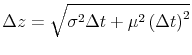
We can view the Brownian motion process associated with ![]() as the limit of a random walk when the time interval
as the limit of a random walk when the time interval ![]() and the step size
and the step size ![]() go to zero simultaneously according to
go to zero simultaneously according to
![]() . Following Bertola and Caballero (1990) , we approximate the continuous-time process with a discrete-time,
discrete state-space Markov chain. Namely, we discretize the
. Following Bertola and Caballero (1990) , we approximate the continuous-time process with a discrete-time,
discrete state-space Markov chain. Namely, we discretize the ![]() state space into
state space into ![]() points with an implied step size that satisfies
points with an implied step size that satisfies
 . Given the step size and time interval, the probability of
 ![]() increasing by
increasing by ![]() is given by
is given by
![]() unconditionally, by
unconditionally, by
![]() conditionally on a positive aggregate shock, and by
conditionally on a positive aggregate shock, and by
![]() conditionally on a negative aggregate shock. The probability of a positive aggregate shock is given by
conditionally on a negative aggregate shock. The probability of a positive aggregate shock is given by
![]() , where
, where
 . Similarly to the continuous-time case, for given values of
 ![]() and
and ![]() , we can find the firm's discrete-time ergodic distribution. When
, we can find the firm's discrete-time ergodic distribution. When ![]() , the discrete-time density is defined as17
, the discrete-time density is defined as17
The job creation rate is defined as18
![]() 19
19

![\displaystyle =\left[ E\left( jc\right) _{d}\right] ^{2}\left\{ p_{a}\left[ \frac{q_{a}\left( q_{z\mid b}-q_{z\mid r}\right) }{q_{z}}\right] ^{2} +q_{a}\left[ \frac{p_{a}\left( q_{z\mid r}-q_{z\mid b}\right) }{q_{z} }\right] ^{2}\right\}](img122.gif) |
||
![\displaystyle \rightarrow\left[ E\left( jc\right) _{c}\right] ^{2}\frac{\sigma_{a} ^{2}}{\sigma^{2}}=Var\left( jc\right) _{c}](img124.gif) . . |
where the second line uses
C. Decompositions of Variances and Covariances
For the decomposition in equation (4), we assume that the employment share of each class is constant over time, so that
Similarly, the decomposition for the covariance between job creation and job destruction, which we use to adjust
![]() in expression (2), is given by
in expression (2), is given by
The decomposition of the coefficient of correlation between aggregate gross job follows and each class gross job flows, for the case of job creation and class 1, is given by
Bibliography
"A Comparison of Job Creation and Job Destruction in Canada and the United States," Review of Economics and Statistics , 80 (3), 347-56. "Kinked Adjustment Costs and Aggregate Dynamics," in O. Blanchard and S. Fischer (eds.), NBER Macroeconomics Annual, MIT Press, Cambridge, MA, 237-88. "What Hides Behind an Unemployment Rate: Comparing Portuguese and U.S. Labor Markets," American Economic Review, 91 (1), 187-207. "Is Job Turnover Countercyclical?," Journal of Labor Economics, 14 (4), 603-25. "The Reallocation of Labour and the Lifecycle of Firms," Oxford Bulletin of Economics and Statistics, 62 (Special Issue), 885-907. "Idiosyncratic Risk and Aggregate Employment Dynamics," Review of Economic Dynamics, 7 (2), 331-53. "Gross Job Creation and Destruction: Microeconomic Evidence and Macroeconomic Implications," in O. Blanchard and S. Fischer (eds.), NBER Macroeconomics Annual, MIT Press, Cambridge, MA, 123-68. "Gross Job Creation, Gross Job Destruction, and Employment Reallocation," Quarterly Journal of Economics, 107 (3), 819-63. "Gross Job Flows," in O. Ashenfelter and D. Card (eds.), Handbook of Labor Economics, Vol. IIIB, Elsevier, Amsterdam, 2711-805. Job Creation and Destruction, MIT Press, Cambridge, MA. The Art of Smooth Pasting, Harwood Academic Publishers, Chur, Switzerland. "Trend Employment Growth and the Bunching of Job Creation and Destruction," Quarterly Journal of Economics, 113 (3), 809-34. "Firm-Specific Learning and the Investment Behavior of Large and Small Firms," International Economic Review, 44 (2), 599-625.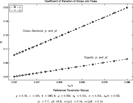
| Year | ||||||
|---|---|---|---|---|---|---|
| 1987 | 6.9 | 12.3 | 5.1 | 8.9 | 3.4 | 21.2 |
| 1988 | 8.0 | 14.3 | 5.3 | 9.0 | 5.3 | 23.2 |
| 1989 | 8.4 | 15.2 | 5.6 | 8.7 | 6.5 | 23.9 |
| 1990 | 7.6 | 13.1 | 6.4 | 10.1 | 2.9 | 23.2 |
| 1991 | 7.5 | 13.7 | 7.5 | 11.1 | 2.5 | 24.8 |
| 1992 | 6.9 | 12.1 | 7.3 | 10.8 | 1.3 | 22.9 |
| 1993 | 5.9 | 11.2 | 8.9 | 13.1 | -1.9 | 24.4 |
| 1994 | 5.2 | 11.3 | 6.8 | 11.1 | 0.2 | 22.4 |
| 1995 | 7.2 | 11.9 | 6.9 | 10.8 | 1.1 | 22.7 |
| 1996 | 7.8 | 12.3 | 6.9 | 10.6 | 1.6 | 22.9 |
| 1997 | 9.1 | 13.9 | 6.4 | 9.9 | 4.1 | 23.8 |
| 1998 | 9.1 | 14.4 | 6.5 | 10.6 | 3.8 | 25.0 |
| 1999 | 9.0 | 13.9 | 6.7 | 11.0 | 2.9 | 25.0 |
Notes:
Notes:
| Size | esh |
|
|
|
|
|
|
|
|---|---|---|---|---|---|---|---|---|
| Overall Economy: 1-49 | 47.6 | 9.2 | 7.1 | 0.14 | 0.10 | 0.58 |
|
|
| Overall Economy: |
52.4 | 6.3 | 6.1 | 0.22 | 0.22 | 0.06 |
|
|
| Overall Economy: |
100.0 | 7.6 | 6.6 | 0.15 | 0.15 |
|
||
| Manufacturing: 1-99 | 51.3 | 7.9 | 6.2 | 0.19 | 0.14 | 0.67 |
|
|
| Manufacturing: |
48.7 | 4.6 | 6.3 | 0.17 | 0.26 | -0.75 |
|
|
| Manufacturing: |
100.0 | 6.2 | 6.2 | 0.15 | 0.19 |
|
||
| Services: 1-24 | 51.0 | 9.0 | 7.1 | 0.10 | 0.08 | 0.40 |
|
|
| Services: |
49.0 | 10.3 | 5.9 | 0.25 | 0.25 | 0.55 |
|
|
| Services: |
100.0 | 9.6 | 6.5 | 0.17 | 0.14 |
|
||
| Retail Trade: 1-9 | 51.0 | 7.9 | 6.5 | 0.10 | 0.08 | 0.37 |
|
|
| Retail Trade: |
49.0 | 10.6 | 5.8 | 0.18 | 0.15 | 0.70 |
|
|
| Retail Trade: |
100.0 | 9.2 | 6.2 | 0.12 | 0.07 |
|
||
| Transportation and Public Utilities: 1-999 | 38.7 | 8.4 | 5.9 | 0.20 | 0.28 | 0.05 |
|
|
| Transportation and Public Utilities:
|
61.3 | 1.3 | 5.4 | 0.18 | 0.87 | -0.80 |
|
|
| Transportation and Public Utilities: |
100.0 | 4.1 | 5.5 | 0.44 | 0.60 |
|
Notes:
| Age: | esh |
|
|
|
|
|
||
|---|---|---|---|---|---|---|---|---|
| Overall Economy: 1-24 | 48.7 | 10.4 | 7.0 | 0.14 | 0.10 | 0.63 |
|
|
| Overall Economy: |
51.3 | 5.2 | 6.6 | 0.20 | 0.21 | -0.31 |
|
|
| Overall Economy: |
100.0 | 7.7 | 6.7 | 0.15 | 0.15 |
|
||
| Manufacturing: 1-27 | 48.9 | 8.8 | 5.7 | 0.19 | 0.15 | 0.65 |
|
|
| Manufacturing: |
51.1 | 3.9 | 7.0 | 0.19 | 0.22 | -0.70 |
|
|
| Manufacturing: |
100.0 | 6.3 | 6.3 | 0.16 | 0.19 |
|
||
| Services: 1-19 | 51.5 | 11.4 | 7.3 | 0.16 | 0.09 | 0.77 |
|
|
| Services: |
48.5 | 8.0 | 8.1 | 0.19 | 0.24 | 0.07 |
|
|
| Services: |
100.0 | 9.8 | 6.7 | 0.16 | 0.14 |
|
||
| Retail Trade: 1-17 | 50.4 | 10.1 | 6.4 | 0.12 | 0.09 | 0.63 |
|
|
| Retail Trade: |
49.6 | 8.7 | 6.2 | 0.21 | 0.13 | 0.69 |
|
|
| Retail Trade: |
100.0 | 9.4 | 6.3 | 0.12 | 0.07 |
|
||
| Transportation and Public Utilities: 1-34 | 21.5 | 11.9 | 6.3 | 0.18 | 0.20 | 0.59 |
|
|
| Transportation and Public Utilities: |
78.5 | 1.9 | 5.5 | 0.63 | 0.76 | -0.85 |
|
|
| Transportation and Public Utilities: |
100.0 | 4.1 | 5.6 | 0.44 | 0.62 |
|
Notes: See table 3.