
Factor Intensity and Price Rigidity:
Evidence and Theory
Keywords: Price rigidity, wage rigidity, factor intensity
Abstract:
Introduction
1.1 Motivation
This paper seeks to understand how industry characteristics can explain observed differences in the degrees of price stickiness across sectors. Using disaggregated data I establish that there is an inverse relationship between the degree of labor intensity and the degree of price flexibility across industries. A model economy, with sticky wages and two sectors which differ in labor intensity, provides theoretical insights on the cause of this relationship. The main finding is that, in an economy with staggered nominal wage contracts, the response of economic variables to unexpected monetary policy shocks varies with the sectoral labor intensity. Wages represent a bigger share of the production cost for the labor-intensive sector, and since nominal wages are fixed, an unexpected monetary policy shock affects the marginal cost in this sector to a lesser extent than the marginal cost in the capital-intensive sector. As a result, in response to an expansionary monetary policy shock for example, the nominal prices of labor-intensive goods increase less than do the prices of capital-intensive goods.
In this setup, firms in both sectors will set new profit-maximizing prices every period, even if the changes they have to make are very small. But assuming some cost to change the price, whether through menu costs or incomplete information, brings some degree of price stickiness into the economy. How long a firm will leave its price unchanged will depend on the loss of profit from not adjusting and the cost of updating the price. Nominal disturbances have bigger effects on the marginal cost of a capital- intensive firm. As a result, the pre-set price of the capital-intensive firm will be farther away from the new profit-maximizing price than it will be for the labor-intensive firm. Thus, firms in the-capital intensive industries face relatively large profits losses if they keep their pre-set prices. The model with costly price adjustment then suggests that firms in the capital-intensive sector will rationally choose to update prices more frequently than firms in the labor-intensive sector. With monetary policy shocks being one of the sources of real and nominal changes in economic variables, this latter finding provides a possible explanation of the empirical result that there is an inverse relationship between the degree of labor intensity and the frequency of price changes across sectors.
Three empirical findings have motivated this work. First, numerous studies1 indicate that the frequency of nominal price changes differs significantly across sectors of the economy. For some goods and services the nominal price remains unchanged for years, while for others the price lasts less than a month. The evidence suggesting sticky prices has motivated the assumption of general nominal price stickiness in the Keynesian models. In these models, monetary policy shocks have real effects. In the opposite direction, the neoclassical literature relies on evidence2 of flexible nominal prices of relatively homogenous commodities like food, gasoline, and computers, and assumes prices to be perfectly flexible.
Second, with regard to wages, Taylor (1999) summarizes the direct and indirect evidence on wage stickiness and concludes that one-year wage contracts are the most common setting for the United States and are prevalent for both union and non-union workers.3
Third, production sectors vary in factor intensity. Based on a sectoral input-output database, Jorgenson and Stiroh (2000) provide data on the values of output and inputs employed by 35 industrial sectors in the United States. The share of labor, for example, varies from 0.09 in the Petroleum and Coal Products industry to 0.5 in the Trade industry.
The empirical evidence that factor intensities vary significantly across sectors, along with the findings on wage and price setting, suggest looking for a relationship between the share of labor input and price stickiness. Ohanian, Stockman, and Kilian (1995) show that the real effects of monetary disturbances differ across sectors because of variation in the degree of price stickiness. At the same time most analyses4 of the transmission of nominal disturbances and optimal monetary policy are based on single-sector models where all firms follow the same price-setting rules.
The economy in the current study has two production sectors: a labor-intensive sector and a capital-intensive sector. Producers in both sectors face menu costs. The labor market is characterized by differentiated labor inputs, supplied by households behaving as monopsonists, wages are assumed to stay fixed for a year, and the wage setting is asynchronous.
The contributions of this study can be summarized as follows: First, it establishes an inverse empirical relationship between the degree of labor intensity and the degree of price flexibility across sectors. Second, this paper shows that models with costly price adjustment, staggered wage contracts, and multiple sectors that differ in factor intensities can generate different degrees of price stickiness across sectors that face the same degree of wage rigidity. More important, such models suggest the same inverse relationship between the degree of labor intensity and the degree of price flexibility as found in the data. Therefore, heterogeneous production functions and sticky wages may be essential features missing in macroeconomic models based on nominal rigidities with exogenous price stickiness.
1.2 Connections to existing literature
Among the papers presenting evidence for considerable nominal stickiness are: Carlton (1986), Cecchetti (1986), Kashyap (1995), and more recently MacDonald and Aaronson (2001). Cecchetti (1986) studies the prices of newsstand magazines over 1953 to 1979 and finds that the average number of years between two consecutive price changes ranges from 1.8 to 14. Kashyap (1995) studies the monthly prices of big revenue items for three retail catalog companies and finds that nominal prices are typically fixed for more than one year. These results contrast with Bils and Klenow's (2004) finding that price changes are much more frequent. Using unpublished data from the U.S. Bureau of Labor Statistics (BLS) for 1995 to 1997, their study shows that half of the prices last 4.3 months or less for consumer goods and services comprising around 70% of the entry level items included in the Consumer Price Index (CPI). In addition, Bils and Klenow (2004) show that the mean duration between price changes varies between 0.6 and 80 months for the separate goods and services. Nakamura and Steinsson (2008) use a more detailed dataset and find that temporary sales play an important in generating price flexibility for retail prices. They estimate that the median duration of regular (non-sale) prices, excluding product substitutions, is between 8 and 11 months but only about 4.5 months when sales are included.
The lack of unanimous results and conclusive evidence on the nominal price rigidity has motivated the search for possible product characteristics that might predict whether a good has a sticky vs. flexible price. Carlton (1986) and Caucutt, Gosh and Kelton (1999) use the inverse of the concentration ratio as a measure for market competition and find a positive relationship between the degree of market competition and the frequency of price changes. Bils and Klenow (2004) look at different variables related to market competitiveness: the wholesale mark-up, the import share, and the rate of introducing substitute products. They conclude that prices change more frequently when there is greater product turnover and that price changes are more common for raw goods. Barsky, House and Kimball (2003), construct a model with durable and non-durable goods, in which only the durable goods have flexible prices because of their infinite intertemporal elasticity of substitution. Erceg and Levin (2002) study the sectoral differences in responses to monetary policy and find that the durable goods sector is more interest sensitive than the non-durables sector.
To improve the performance of Taylor (1980)- and Calvo (1983)- type models and account for the varying price flexibility, models of multi-sector economies have been studied by Blinder and Mankiw (1984), Ohanian, Stockman and Kilian (1995), and Bils, Klenow and Kryvtsov (2003). In these models, sectors are differentiated by different degrees of price flexibility. Goods and services are divided into sectors with exogenously determined nominal price rigidity after observing the frequency of price changes in the data.
Similarly to the above papers, I look for an explanation for the different nominal stickiness across sectors, but I look at the labor and capital intensities as the source of these differences. In contrast to the above models, the economy I study in the first part of this paper does not impose price stickiness exogenously, but it assumes that nominal wages are fixed for a certain time period and producers face a cost of setting a new price. As a result nominal disturbances affect the labor-intensive and the capital-intensive sectors asymmetrically: prices of labor-intensive goods change less than do prices of capital-intensive goods. The relationship between staggered wages and the responses of prices and output to monetary policy shocks is also explored by Olivei and Tenreyro (2007), not across sectors but across the quarters of the year. They show that the response of output depends on the timing of the monetary policy shock. When the shock occurs during the first two quarters, the response of the output is quick and dies out relatively fast. The authors' explanation is the uneven staggering of wage contracts across quarters.
To obtain different frequencies of price adjustments rather than different magnitudes of price responses between the different sectors, in the second part of this paper I assume that it is costly to change prices. I utilize a one-period model with menu costs that generally follows Blanchard and Kiyotaki (1987) but adds capital as a factor of production and allows for two sectors that differ in factor intensity. When firms face menu costs, some of them optimally choose not to adjust their prices. Only firms for which the expected loss of profit is bigger than the menu cost will pay this cost and will adjust their prices. Menu costs have often been suggested as a possible explanation for staggered prices. Both Mankiw (1985) and Blanchard and Kiyotaki (1987) find that small menu costs can prevent firms from adjusting their prices and thus cause large changes in output and welfare in response to changes in nominal money. Similarly to these papers, the model I construct shows that small menu costs (of second order) can prevent firms from changing their prices. In addition, I obtain the following result: if the labor-intensive sector and the capital-intensive sector face the same distribution of menu costs, a larger fraction of firms in the capital-intensive sector will pay the menu cost and will adjust their prices in response to a change in the money supply. This is consistent with the empirical finding that motivated this paper because it implies that in any given period characterized by a nominal disturbance, the probability of a capital-intensive firm changing its price is higher than the probability of a labor-intensive firm doing the same.
Nominal wage rigidity, which is the same across sectors, is important for my main result. The latter finding is in line with the work of Erceg (1997), Chari, Kehoe and McGratten (2000), and Huang and Liu (2002), whose conclusions are that staggered wages are an important feature in Keynesian models, in which monetary shocks have real effects due to staggered contracts. It should be noted that these authors reach this conclusion because models with staggered prices alone can not generate the observed persistent output fluctuations, whereas this paper finds that wage stickiness is important because it can also explain the wide range of price flexibility in the data.
2. Data on Labor Intensity and Frequency of Price Changes
Intrigued by the dramatic range of the price change frequencies in their data set, Bils and Klenow (2004) match most of the Entry Level Items (ELIs), comprising 68.9% of the CPI, to 123 National Income and Product Accounts (NIPA) categories.5 This allows them to use the NIPA time series on prices and study the correlation between the frequency of price changes and the persistence and volatility of inflation across the goods categories. They do not find evidence in support of the relation between inflation behavior and the frequency of price changes predicted by the sticky-price models of the Calvo- and Taylor-type. The main focus of their paper is the pricing equation derived in these models. I will use their data but will focus on the relationship between labor intensity and frequency of price changes.
Similarly to Bils and Klenow (2004), I will group the ELIs using, however, the Standard Industrial Classification (SIC) classification, i.e. the goods are divided according to the industry by which they are produced. The motivation for this division comes from the observation that in the bottom 10th percentile of the Bils and Klenow (2004) data (i.e. the ELIs whose prices change least often - less than once a year), 82.6% are services, an industrial category characterized by relatively high labor intensity. On the other hand, among the10 percent of the goods and services with the most flexible prices, only 7.6% are services. So it is interesting to see whether labor intensity might explain why the prices of dry cleaning, newspapers, vehicle inspection, and other similar services change once every 4-5 years, while the prices of gasoline and tomatoes on average remain unchanged for less than a month.
To examine the relationship between the frequency of price changes and the labor/capital intensity I would need data on how much labor and capital is used for the production of each good and service included in the CPI. Such disaggregate data are not available, but Jorgenson and Stiroh (2000) provide a database developed by Dale W. Jorgenson that covers 35 sectors at the 2-digit SIC level and contains information on the value of employed inputs (capital, labor, materials and energy) as well as the value of output for each industrial sector for 1958 to 1996.
Using the SIC system, I match the 350 ELIs to the manufacturing industries (as defined in the Jorgenson's database) in which these goods and services were produced. The ELIs can be matched to 29 out of the 35 sectors but many of the SIC sectors are broader. Table A1 in Appendix A shows the industrial sectors and the number of items in each sector. In addition, the table shows the weighted average monthly frequency of a price change for each industry. These frequencies are weighted means of the category components, with weights given by the share of each ELI in the 1995 Consumer Expenditure Survey.
Figure 1 plots the weighted mean monthly frequencies of a price change and the share of labor input for each of the 29 industries (an average of the shares of labor inputs for the years from 1958 to1996). Sectors with high labor share in output tend to change the prices of their products less often.
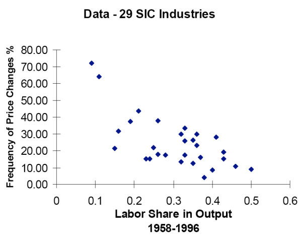
Table 1 reports the results of the weighted least squares regression of price-change frequencies on labor shares. The weight given to each industry is again calculated using weights of the ELIs belonging to that industry sector, namely the goods' importance in 1995 consumer expenditure, reported by Bils and Klenow (2004). The labor share is obtained from the Jorgenson database and is defined as the value of labor divided by the sum of the values of labor, capital, energy and materials.
Table 1. Weighted Least Squares
(Dependent variable: Average monthly frequency of price changes)
| Coefficients | Standard Error | t Stat | P-value | Lower 95% | Upper 95% | |
|---|---|---|---|---|---|---|
| Intercept | 0.36 | 0.0478 | 7.5702 | 0.0000 | ||
| Labor share | -0.57 | 0.1758 | -3.2399 | 0.0032 | -0.9389 | -0.1965 |
| Adjusted R2 | 0.9343 |
A weighted least squares (WLS) regression produces an economically and statistically significant negative relationship between the labor intensity and the frequency of price changes6. The coefficient of -0.57 implies that an increase in the labor share from 0.17 for food and kindred products to 0.50 for instruments will decrease the monthly frequency of price change by around 20 percentage points. In the data the frequencies are 31.53% and 10.85% respectively. I also consider one more variable in a separate regression - product turnover. Bils and Klenow (2004) find this variable to robustly predict more frequent price changes7. To see whether it will be a good predictor when goods are split in industries of origin, I calculate a weighted mean product turnover for each industry. When added as an explanatory variable to the regression of price-change frequencies on labor shares, the coefficient on the rate of product turnover is statistically and economically insignificant. At the same time the coefficient on labor share remains unchanged8.
For comparison, I also checked if there is a similar significant relationship between the frequency of price changes and the rest of the inputs: energy, capital, and materials9. There is a positive but unstable relationship between the share of materials and the frequency of price changes. It exists if several outliers are removed from the data set, but turns negative if I take out the labor-intensive sectors. With respect to energy and capital, I do not find support for any significant relationship.
This preliminary analysis suggests that different degrees of labor intensity across sectors might play an important role in the Keynesian model with nominal rigidities. In the next section I develop a theoretical model to analyze the effects of nominal wage stickiness in an economy with two sectors which differ in their labor intensity.
3. Overview of the Model
In this section, I construct a two-sector dynamic general equilibrium model with money in the utility function and different degrees of labor intensity across sectors. My intent was not to match particular features of the data, but to clearly understand the effects of monetary policy shocks on labor, real output, marginal costs, and prices in such a model, and more importantly, to see whether the model can help explain why some firms change their prices frequently while others have sticky nominal prices. The optimization problems of firms, intermediaries, and households are described in detail and the conditions for market equilibrium are defined.
The model closely follows and modifies Huang and Liu (2002), which is a one sector, staggered-wage monetary business cycle model. The economy is populated by a continuum of infinitely lived households distributed over the unit interval, and each one acts as a monopolistic supplier of differentiated labor services. In the labor market, wages are determined in a staggered fashion. Nominal wages are fixed for one year, and households agree to supply their differentiated labor input so that demand is satisfied at this wage. Every six months, one-half of the households are allowed to adjust their nominal wages, making the wage-setting asynchronous. The wage-setting process is derived from the households' optimization problem. In addition each household consumes some of the final output, rents and invests in capital and holds money balances. For ease of analysis I assume that an intermediary hires all of the differentiated labor inputs and supplies competitively an aggregate labor index using the same proportions that firms would choose.
There are two goods-producing sectors in this economy. Each of the two sectors has a continuum of monopolistically competitive intermediate firms, which hire aggregate labor from the intermediary and capital from the households to produce differentiated products. The labor and capital inputs are not sector-specific and there is no restriction on the flow of resources between the two sectors. An important feature of this model is that firms in the first sector have a labor-intensive production and the firms in the second have a capital-intensive one. Similarly to the labor intermediary, a representative aggregator for each sector competitively produces a consumption good by combining the continuum of all firms' differentiated products, using the same proportions that households would choose.
The monetary authority governs the nominal money supply process by setting its growth rate according to some exogenous process.
3.1 Final Good Production
The final aggregate good is produced by applying the following constant elasticity of substitution (CES) technology:
The firm produces the final aggregate good competitively. In each period ![]() , it chooses the quantity of
, it chooses the quantity of ![]() and
and ![]() taking as given their nominal prices,
taking as given their nominal prices, ![]() and
and ![]() 10
respectively, to maximize profits subject to the production function. Specifically, the firm solves the following optimization problem:
10
respectively, to maximize profits subject to the production function. Specifically, the firm solves the following optimization problem:
The zero profit condition gives the price index (also the aggregate price level):
3.2 The Representative Firms in the Two Sectors
The consumption goods ![]() and
and![]() , produced competitively by a representative
firm in sector one and sector two, are Dixit and Stiglitz (1977) composites of differentiated intermediate goods indexed by
, produced competitively by a representative
firm in sector one and sector two, are Dixit and Stiglitz (1977) composites of differentiated intermediate goods indexed by ![]() in sector one , and by
in sector one , and by ![]() in sector two. Because households have identical preferences, the intermediate goods are combined using the same proportions that the households would choose. In each period
in sector two. Because households have identical preferences, the intermediate goods are combined using the same proportions that the households would choose. In each period ![]() , the representative firms, taking prices as given, choose the intermediate inputs
, the representative firms, taking prices as given, choose the intermediate inputs ![]() for all
for all ![]() and
and ![]() for all
for all![]() respectively, to maximize profits subject to the production technology. Intermediate goods
respectively, to maximize profits subject to the production technology. Intermediate goods
![]() can not flow between the two sectors and therefore go to the production of only
can not flow between the two sectors and therefore go to the production of only
![]() , respectively. In sector one the optimization problem is given by:
, respectively. In sector one the optimization problem is given by:
where ![]() is the price of the composite good produced by sector one in period
is the price of the composite good produced by sector one in period ![]() ,
, ![]() and
and ![]() are the price and quantity of the
intermediate good produced by firm
are the price and quantity of the
intermediate good produced by firm ![]() in sector one in period
in sector one in period ![]() , and
, and
![]() is the elasticity of substitution between each of the differentiated products
is the elasticity of substitution between each of the differentiated products![]() .
.
The optimization problem for the representative firm in sector two can be obtained by replacing ![]() with
with ![]() in equations (6) and (7).
in equations (6) and (7). ![]() will be the price of the composite good produced by sector two in period
will be the price of the composite good produced by sector two in period ![]() , and
, and ![]() and
and ![]() - the price and quantity of the intermediate good produced by firm
- the price and quantity of the intermediate good produced by firm ![]() in sector two in period
in sector two in period ![]() .
.
The representative firms' optimization problems yield the demand functions for every intermediate product ![]() in sector one and every intermediate product
in sector one and every intermediate product ![]() in sector two at time
in sector two at time ![]() :
:
The zero-profit conditions imply that the price indices are given by:
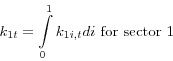
![\begin{displaymath} P_{1t} =\left[ {\int\limits_0^1 {P_{1i,t}^{\frac{-\theta }{1-\theta }} di} } \right]^{-\frac{1-\theta }{\theta }} \end{displaymath}](img35.gif)
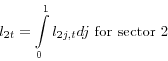
![\begin{displaymath} P_{2t} =\left[ {\int\limits_0^1 {P_{2j,t}^{\frac{-\theta }{1-\theta }} dj} } \right]^{-\frac{1-\theta }{\theta }} \end{displaymath}](img36.gif)
3.3 The Intermediate Firms
There is a continuum of monopolistically competitive intermediate firms in sector one and two. They sell their differentiated products![]() ,
,![]() and
and ![]() ,
,![]() to the representative firms. All the firms within a sector have identical production functions. The only difference between the two production sectors is that production in sector one is labor-intensive, while production in sector two is capital intensive. The technology for
producing each unique intermediate good is a standard Cobb-Douglas production function given as:
to the representative firms. All the firms within a sector have identical production functions. The only difference between the two production sectors is that production in sector one is labor-intensive, while production in sector two is capital intensive. The technology for
producing each unique intermediate good is a standard Cobb-Douglas production function given as:
where
![]() and
and
![]() are the share of capital in costs, with
are the share of capital in costs, with ![]()
![]()
![]() ;
; ![]()
![]() and
and ![]()
![]() are the capital and labor inputs used to produce the intermediate good
are the capital and labor inputs used to produce the intermediate good ![]() and
and
![]() , respectively. At time
, respectively. At time ![]() , each monopolistic firm
, each monopolistic firm ![]() in sector one and firm
in sector one and firm ![]() in sector two, taking as given the nominal wage (
in sector two, taking as given the nominal wage (![]() and nominal rent on capital (
and nominal rent on capital (![]() , choose the quantity of output and correspondingly the amount of labor and capital
inputs to maximize profits, subject to the production function and the demand for their product. When choosing the quantity of output, each firm takes into account that the decision will not affect the aggregate demand for their sector. That is each firm solves one of the following problems,
depending on what sector they are part of:
, choose the quantity of output and correspondingly the amount of labor and capital
inputs to maximize profits, subject to the production function and the demand for their product. When choosing the quantity of output, each firm takes into account that the decision will not affect the aggregate demand for their sector. That is each firm solves one of the following problems,
depending on what sector they are part of:
Firm ![]() in sector one solves:
in sector one solves:
![\begin{displaymath} \begin{array}{c} \mbox{Max } P_{1i,t} y_{1i,t} -(R_t .k_{1i,t} +W_t .l_{1i,t} ) \\ \ \par \mbox{s.t. } y_{1i,t} \le k_{1i,t}^\alpha l_{1i,t}^{1-\alpha } \\ \ \par y_{1i,t} =\left[ {\frac{P_{1t} }{P_{1i,t} }} \right]^{\frac{1}{1-\theta}}y_{1t} \end{array}\end{displaymath}](img50.gif)
Firm ![]() in sector two solves:
in sector two solves:
![\begin{displaymath} \begin{array}{c} \mbox{Max } P_{2j,t} y_{2j,t} -(R_t .k_{2j,t} +W_t .l_{2j,t} )\\ \ \mbox{s.t. } y_{2j,t} \le k_{2j,t}^\gamma l_{2j,t}^{1-\gamma }\\ \ y_{2j,t} =\left[ {\frac{P_{2t} }{P_{2j,t} }} \right]^{\frac{1}{1-\theta }}y_{2t} \end{array}\end{displaymath}](img51.gif)
Because all firms in the economy face the same prices for their inputs, labor and capital, and because all firms within a sector have access to the same homogenous-of-degree-one production functions, the above optimization problems imply equal capital-labor ratios across the intermediate firms within a sector but different between the two sectors:
The first order conditions also give the input demand functions of each firm for labor and capital. The demand for labor and capital by firms in sector one and two is given by the following four equations, respectively:
and
Since the firms in both sectors are monopolistically competitive they set their prices as a constant mark-up over their nominal marginal cost. The size of the mark-up is directly related to the degree of substitution between the intermediate goods (i.e. the degree of monopoly power). Lower
![]() means smaller elasticity of substitution
means smaller elasticity of substitution
![]() , higher monopoly power, and higher mark-up
, higher monopoly power, and higher mark-up
![]() .
.
For example the price any firm ![]() in sector one sets is:
in sector one sets is:
where ![]() and
and![]() are the marginal products of labor and capital, and
are the marginal products of labor and capital, and
![]() is the nominal marginal cost for firm
is the nominal marginal cost for firm ![]() in sector one. The pricing equation
for a firm in sector two will be identical except for the parameter
in sector one. The pricing equation
for a firm in sector two will be identical except for the parameter![]() , which will be replaced by
, which will be replaced by![]() .
.
To obtain the total demand of the capital-intensive and labor-intensive sectors for capital and labor input, we integrate over all firms within each sector:
and
Total capital and labor inputs, available in the economy, are allocated between the two sectors according to the following two relationships:
In summary, the relationship between the input factors is the following: in sector one each firm's labor and capital demand is given by ![]() and
and ![]() , respectively. The aggregate demand for labor by sector one is
, respectively. The aggregate demand for labor by sector one is ![]() , as defined in (23), and the aggregate
demand for capital is
, as defined in (23), and the aggregate
demand for capital is ![]() , as defined in (24). The relationships in sector two can be obtained by replacing
, as defined in (24). The relationships in sector two can be obtained by replacing ![]() with
with![]() . To derive the total demand for capital,
. To derive the total demand for capital, ![]() ,
one has to add the demand by the two sectors as shown in (27). The total demand for the aggregate labor index,
,
one has to add the demand by the two sectors as shown in (27). The total demand for the aggregate labor index, ![]() , is similarly obtained in (28).
, is similarly obtained in (28).
3.4 The Labor Aggregating Firm
For ease of analysis I introduce a labor supplying firm. It acts competitively and aggregates the differentiated labor skills ![]() , supplied by a continuum of households
, supplied by a continuum of households
![]() , and then sells the aggregate index to intermediate good-producing firms from the two sectors. The firm takes as given the wage rate
, and then sells the aggregate index to intermediate good-producing firms from the two sectors. The firm takes as given the wage rate ![]() , set by each household, and minimizes the cost of obtaining aggregate labor
, set by each household, and minimizes the cost of obtaining aggregate labor ![]() , subject to the production
function:
, subject to the production
function:
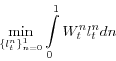
![\begin{displaymath} \mbox{s.t. } \left[ {\int\limits_0^1 {(l_t^n )^{\frac{\sigma -1}{\sigma }}} dn} \right]^{\frac{\sigma }{\sigma -1}}\ge l_t \end{displaymath}](img79.gif)
where ![]()
![]() 1 is the elasticity of substitution between each of the
differentiated labor skills.
1 is the elasticity of substitution between each of the
differentiated labor skills.
From the optimization problem the following demand for labor input ![]() is derived:
is derived:
where ![]() , the aggregate wage, is set competitively by the labor aggregating firm and is given by:
, the aggregate wage, is set competitively by the labor aggregating firm and is given by:
![\begin{displaymath} W_t =\left[ {\int\limits_0^1 {\left( {W_t^n } \right)^{1-\sigma }dn} } \right]^{\frac{1}{1-\sigma }} \end{displaymath}](img84.gif)
3.5 Households
The economy is populated by a continuum of households indexed by
![]() . Each household is endowed with a differentiated labor skill and faces a downward-sloping demand for its own type of skill. In what follows I apply the staggered
nominal wage-setting process originally developed in Taylor (1979, 1980)11 and assume two-period Taylor-type wage staggering. Households are divided into 2
cohorts based on the timing of their wage decision. I assume that only a fraction
. Each household is endowed with a differentiated labor skill and faces a downward-sloping demand for its own type of skill. In what follows I apply the staggered
nominal wage-setting process originally developed in Taylor (1979, 1980)11 and assume two-period Taylor-type wage staggering. Households are divided into 2
cohorts based on the timing of their wage decision. I assume that only a fraction ![]() of all households set their wages in a given period and this wage is fixed for the 2 subsequent periods.
The households indexed
of all households set their wages in a given period and this wage is fixed for the 2 subsequent periods.
The households indexed
![]() set new wages in periods
set new wages in periods
![]() , i.e. at time
, i.e. at time ![]() ,
, ![]() + 2,
+ 2, ![]() + 4, etc. Similarly, households indexed
+ 4, etc. Similarly, households indexed
![]() set new wages at time
set new wages at time ![]() +1,
+1, ![]() +3,
+3, ![]() + 5, or periods
+ 5, or periods
![]() . Each household is assumed to always meet the demand for its labor type at the wage it has chosen. In period
. Each household is assumed to always meet the demand for its labor type at the wage it has chosen. In period ![]() a household
a household ![]() takes as given the gross inflation rate, the gross nominal interest rate
takes as given the gross inflation rate, the gross nominal interest rate![]() on a one period nominal bond between today and tomorrow, the rental rate on capital, the real wage rate on aggregate labor index, the aggregate labor demand and the wage stickiness. Subject to several constraints, the household chooses
consumption
on a one period nominal bond between today and tomorrow, the rental rate on capital, the real wage rate on aggregate labor index, the aggregate labor demand and the wage stickiness. Subject to several constraints, the household chooses
consumption![]() of the economy's single final good, real money balances
of the economy's single final good, real money balances
![]() , the capital stock, and if allowed - the nominal wage rate
, the capital stock, and if allowed - the nominal wage rate![]() ,
to maximize the total discounted expected utility. Thus the optimization problem of households able to reset their wage in periods
,
to maximize the total discounted expected utility. Thus the optimization problem of households able to reset their wage in periods
![]() is the following:
is the following:
![\begin{displaymath} \mathop {\max }\limits_{\{c_t^n ,\frac{M_t^n }{P_t },W_t^n ,k_{t+1}^n \}} E_0 \left\{ {\sum\limits_{t=0}^\infty {\beta ^t[} U(c_t^n ,M_t^n /P_t ,l_t^n )]} \right\} \end{displaymath}](img94.gif)
and equation (31).
Equation (34) is the budget constraint, (35) represents the wage stickiness restriction, (36) is the law of motion for capital, and (31) is the labor demand schedule. The temporal utility function is given by:
Since not all wages are set at the same time, households in general will receive different wages and supply different amount of labor, depending on whether or not they are allowed to reset their wage rate in a given period. Consequently their wealth will differ and so will their choices for consumption, nominal money balances and capital stock. This will require one to keep track of the income distribution across household cohorts from period to period. To make the model manageable and an analytical solution possible, I will assume that households start with identical initial wealth, and portfolios of state-contingent claims can be constructed so as to provide the household with complete insurance against the idiosyncratic risk. Since households value consumption and real money balances identically and face the same prices, the complete insurance guarantees that equilibrium consumption flows and real money balances will also be identical for all households.
The first order conditions from the households' optimization problem yield the demand for real money balances as a function of consumption and nominal interest rate:
and the Euler condition for the optimal intertemporal allocation of consumption
In equations (38) - (40),
 and
and
![]() is aggregate inflation in period
is aggregate inflation in period ![]() .
.
In addition a household in a wage-setting cohort will choose the following real wage in period ![]() :
:
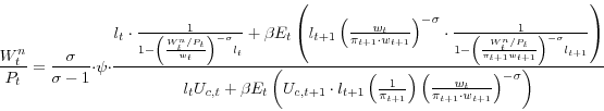
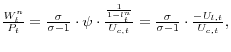 i.e. households, as monopolistic
suppliers of labor, set their wages as a mark-up over the marginal rate of substitution between leisure and consumption for the current period. Since wages are fixed for two subsequent periods, the households set their real wage rates as a constant mark-up
i.e. households, as monopolistic
suppliers of labor, set their wages as a mark-up over the marginal rate of substitution between leisure and consumption for the current period. Since wages are fixed for two subsequent periods, the households set their real wage rates as a constant mark-up
![]() over the ratio of weighted marginal disutility of labor to marginal utilities of consumption for the duration of their wage contracts.
When a household expects an increase in the marginal utility of consumption and/or a decrease in the marginal utility of leisure for the periods its wage is fixed, it chooses a lower nominal wage and supplies more of its labor. Since all households, resetting wage in period
over the ratio of weighted marginal disutility of labor to marginal utilities of consumption for the duration of their wage contracts.
When a household expects an increase in the marginal utility of consumption and/or a decrease in the marginal utility of leisure for the periods its wage is fixed, it chooses a lower nominal wage and supplies more of its labor. Since all households, resetting wage in period ![]() , will choose the same wage, I will denote this wage with
, will choose the same wage, I will denote this wage with ![]() and use it to substitute for
and use it to substitute for
![]() in equation (41). Along with the assumption of two-period wage staggering equation (32) can be rewritten to get an expression for the real aggregate wage
in equation (41). Along with the assumption of two-period wage staggering equation (32) can be rewritten to get an expression for the real aggregate wage ![]() :
:
![\begin{displaymath} w_t =\frac{W_t }{P_t }=\left[ {\frac{1}{2}\left( {\frac{S_t }{P_t }} \right)^{1-\sigma }+\frac{1}{2}\left( {\frac{S_{t-1} }{P_t }} \right)^{1-\sigma }} \right]^{\frac{1}{1-\sigma }}=\left[ {\frac{1}{2}\left( {\frac{S_t }{P_t }} \right)^{1-\sigma }+\frac{1}{2}\left( {\frac{S_{t-1} }{P_{t-1} }\cdot \frac{1}{\pi _t }} \right)^{1-\sigma }} \right]^{\frac{1}{1-\sigma }} \end{displaymath}](img119.gif)
In equations (43) and (44), the cohort of households indexed
![]() can reset their wage in period
can reset their wage in period ![]() , while the rest of
the households can not.
, while the rest of
the households can not.
3.6 The Monetary Authority
The nominal money supply process is given by:
where
3.7 Market Equilibrium
The assumption that there exist complete financial markets along with the market clearing conditions:
 ,
,
 , and
, and
 , allow me to drop the
![]() superscript from
superscript from
![]() and
and ![]() in the households' decisions, when defining the economy's
equilibrium. The households' supply of labor
in the households' decisions, when defining the economy's
equilibrium. The households' supply of labor![]() and wage rate
and wage rate![]() would still be
different among the cohorts but identical for households within a cohort, because in what follows the focus will be on a symmetric equilibrium in which all households, allowed to reset their wage, will chose the same wage rate (
would still be
different among the cohorts but identical for households within a cohort, because in what follows the focus will be on a symmetric equilibrium in which all households, allowed to reset their wage, will chose the same wage rate (![]() and will supply the same amount of labor. At the same time in a symmetric equilibrium, in the absence of price staggering, all firms within the labor-intensive sector will make identical decisions about production, labor and capital inputs, as well as
pricing. Thus, in equilibrium in which equations (7), (23) and (24) hold with equality, the subscript
and will supply the same amount of labor. At the same time in a symmetric equilibrium, in the absence of price staggering, all firms within the labor-intensive sector will make identical decisions about production, labor and capital inputs, as well as
pricing. Thus, in equilibrium in which equations (7), (23) and (24) hold with equality, the subscript ![]() will be omitted from the optimal conditions for
will be omitted from the optimal conditions for![]() ,
, ![]() ,
,![]() , and
, and ![]() . Similarly for the capital-intensive sector the subscript
. Similarly for the capital-intensive sector the subscript ![]() will be dropped from
will be dropped from![]() ,
,![]() ,
,![]() , and
, and ![]() .
.
Then the symmetric equilibrium of the economy will consist of an allocation
![]() and a sequence
and a sequence
![]() such that given the initial values for
such that given the initial values for
![]() and the sequence of monetary policy shocks:
and the sequence of monetary policy shocks:
![]() , the following conditions are satisfied:
, the following conditions are satisfied:
- taking the wage on the aggregate labor, the rental rate on capital and all but its own price as given, the intermediate monopolistic firms in sector one and two solve (14) and (15) respectively,
- taking the price of the composite goods produced by the two sectors as given, the firm producing the final consumption good solves (2),
- taking the wages on the differentiated labor inputs as given, the labor aggregating firm solves (29),
- taking as given the gross inflation rate, the gross nominal interest rate, the rental rate on capital, the real wage rate on aggregate labor index, the aggregate labor demand, and the wage stickiness households solve (33),
- the monetary authority follows (45) and (46),
- the capital market clears (27), the labor market clears (28) and the aggregate resource constraint is satisfied.
In the above definition of symmetric equilibrium, the aggregate resource constraint, the real marginal costs in the labor-intensive sector (![]() and the capital intensive sector
(
and the capital intensive sector
(![]() are given respectively by:
are given respectively by:
A system of 21 non-linear equations defines the equilibrium. I log-linearize these equations around the non-stochastic steady state of the model (see Appendix B for details). This allows the system of non-linear equations to be approximated by a system of linear equations which characterize the dynamics of the model for small deviations around the deterministic steady state. After the log-lineariztaion, the system of equations characterizing the economy can be written as:
4. Parameterization
Table 2. Benchmark Model Parameters
| Preferences |
|
|---|---|
| Production
|
|
| Market Demand
|
|
| Capital accumulation
|
|
| Money Growth
|
|
| Sectors' Weight in Final Output |
The time period in this model is assumed to be six months. The preference parameters in the utility function are basically the ones employed by Huang and Liu (1999). To assign values for![]() and
and![]() , where
, where ![]() is the relative weight of consumption, and
is the relative weight of consumption, and
![]() is the interest rate elasticity of demand for real money holdings, they estimate the following regression for logged money demand:
is the interest rate elasticity of demand for real money holdings, they estimate the following regression for logged money demand:
The values they obtain are very similar to the values Chari at al. (2000) obtain using the same equation and quarterly data. The subjective discount rate used in the utility function,
To analyze the effects of a monetary policy shock in two sectors with different capital and labor shares, I will later assign different values for ![]() and
and![]() . The only restriction will be that the weighted average of
. The only restriction will be that the weighted average of ![]() and
and![]() should still equal 0.33, which will guarantee identical steady state output to capital ratios in the two models. The parameter
should still equal 0.33, which will guarantee identical steady state output to capital ratios in the two models. The parameter ![]() is adjusted so that the share of time households allocate to labor is around 1/3 in the steady state. With these parameters the baseline model predicts annualized output-capital ratio of 0.41, investment-output ratio of 0.19 and consumption-capital ratio of 0.33.
is adjusted so that the share of time households allocate to labor is around 1/3 in the steady state. With these parameters the baseline model predicts annualized output-capital ratio of 0.41, investment-output ratio of 0.19 and consumption-capital ratio of 0.33.
I calibrate the serial correlation parameter for money growth rate![]() following Chari at al. (2000) and Cho and Cooley (1995). They obtain a value for the money growth persistence
of 0.57 by fitting first order auto-regressive process for logged money growth (
following Chari at al. (2000) and Cho and Cooley (1995). They obtain a value for the money growth persistence
of 0.57 by fitting first order auto-regressive process for logged money growth (
![]() using quarterly data on M1.
using quarterly data on M1.
In the benchmark model I set elasticity of substitution in both labor market ![]() and final output market
and final output market ![]() to be 10. An elasticity of substitution of 10 in the output market implies a price mark-up of 11% in the steady state, which is standard in the sticky price literature and is based on the work of Basu and Fernald (1994, 1995).
to be 10. An elasticity of substitution of 10 in the output market implies a price mark-up of 11% in the steady state, which is standard in the sticky price literature and is based on the work of Basu and Fernald (1994, 1995).
There is no standard value in the literature for the elasticity of substitution between the differentiated labor skills. The range of values for![]() in the literature is between 2
[see Griffin (1992, 1996)] and 20 [see Koening (1997)]. The elasticity of substitution is crucial for the persistence of the responses of real variables to monetary policy shocks, but the main results of this paper hold for different values of
in the literature is between 2
[see Griffin (1992, 1996)] and 20 [see Koening (1997)]. The elasticity of substitution is crucial for the persistence of the responses of real variables to monetary policy shocks, but the main results of this paper hold for different values of![]() . For this reason I start with a value that is in the middle of the plausible range and then later experiment with different values. Finally, for ease of analysis, I assume that the two sectors in this economy have equal weight in the
final consumption good by setting
. For this reason I start with a value that is in the middle of the plausible range and then later experiment with different values. Finally, for ease of analysis, I assume that the two sectors in this economy have equal weight in the
final consumption good by setting![]() .
.
5. Findings
Before examining the dynamics of the model, it should be noted that the assumed parameters imply that the two sectors have equal weight in the final consumption good and are symmetric in every way, except for the fact that first is labor-intensive and the second is capital intensive. The intermediate firms from the two sectors pay the same rent on capital, the same wage rates, and face the same elasticity of substitution for their products. Since only the wage contracts are staggered, the monopolistic competition within each sector is not crucial for the results. The presence of monopolistic competition, though, makes the environment in the model comparable to the rest of the existing literature and prepares the model for a relatively easy switch to a staggered-wage, staggered-price model.
5.1 Identical Sectors
Figures 2 and 3 plot the impulse response functions of key economic variables in the benchmark model (
![]() , following a monetary shock that increases the growth rate of money stock by 1 percent. Under staggered wage setting, half of the households can not reset their wage in
response to the monetary shock, and the other half can, but face a decrease in the demand for their labor skills when they choose to set a higher nominal wage. Because of the sticky wages, after the realization of the monetary policy shock, the real aggregate wage decreases (fig.3) and the demand
for labor increases (fig. 2). The simultaneous increase of a household's income and demand for its labor leads to a decrease in the marginal utility of income and an increase in the marginal utility of leisure. Both of these results require that a household sets a higher wage. But given the
staggered nature of the aggregate wage, a household setting a higher nominal wage (and thus a higher relative wage) faces a decline in the demand for its specific labor skills and thus a decrease in income and time spent working. This prevents the wage-setting cohort from increasing their wages the
way they would if every household was allowed to do so, and the final increase in the relative wage is small.
, following a monetary shock that increases the growth rate of money stock by 1 percent. Under staggered wage setting, half of the households can not reset their wage in
response to the monetary shock, and the other half can, but face a decrease in the demand for their labor skills when they choose to set a higher nominal wage. Because of the sticky wages, after the realization of the monetary policy shock, the real aggregate wage decreases (fig.3) and the demand
for labor increases (fig. 2). The simultaneous increase of a household's income and demand for its labor leads to a decrease in the marginal utility of income and an increase in the marginal utility of leisure. Both of these results require that a household sets a higher wage. But given the
staggered nature of the aggregate wage, a household setting a higher nominal wage (and thus a higher relative wage) faces a decline in the demand for its specific labor skills and thus a decrease in income and time spent working. This prevents the wage-setting cohort from increasing their wages the
way they would if every household was allowed to do so, and the final increase in the relative wage is small.
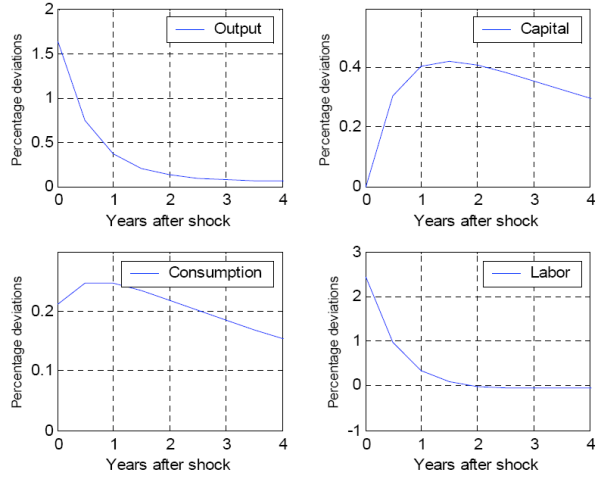
The amount of capital in the economy at date ![]() is chosen at
is chosen at ![]() , in the standard
way, and does not respond to a monetary policy shock realized at date
, in the standard
way, and does not respond to a monetary policy shock realized at date ![]() . The increase in labor, only, leads to an increase in the marginal product of capital and the real rental rate. Output
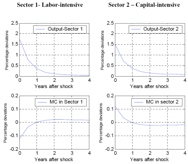
also initially increases, because of the increase in labor, and then gradually returns to steady state. The impulse responses of output, in sectors one and two, are identical to the aggregate output response and for this reason are not included in the graphs below. As Huang and Liu (2002) show,
higher elasticity of substitution between labor skills means a more persistent output response. The intuition behind this relation is that the easier it is to substitute one household's labor skill with a different one, the more reluctant the wage-setting household cohort will be to increase its
nominal wage. The direction of the impulse responses is robust to the choice of elasticity of substitution between differentiated labor inputs. Thus in the benchmark model with two identical sectors, employment, output, consumption and investment (not shown) are pro-cyclical.
. The increase in labor, only, leads to an increase in the marginal product of capital and the real rental rate. Output
also initially increases, because of the increase in labor, and then gradually returns to steady state. The impulse responses of output, in sectors one and two, are identical to the aggregate output response and for this reason are not included in the graphs below. As Huang and Liu (2002) show,
higher elasticity of substitution between labor skills means a more persistent output response. The intuition behind this relation is that the easier it is to substitute one household's labor skill with a different one, the more reluctant the wage-setting household cohort will be to increase its
nominal wage. The direction of the impulse responses is robust to the choice of elasticity of substitution between differentiated labor inputs. Thus in the benchmark model with two identical sectors, employment, output, consumption and investment (not shown) are pro-cyclical.
Investment is more volatile than output, which is more volatile than consumption. This is consistent with the results produced by standard monetary business cycle models without any rigidities. It is worth mentioning a special feature of the benchmark model. As can be seen in the last two panels of fig. 3, real marginal cost does not respond to the monetary policy shock in either sector. This is due to the fact that capital is fixed, and when the real aggregate wage decreases and labor supply increases, the rental rate on capital increases just enough to offset the reduction in the real wage and the increase in labor supply, thus leaving real marginal cost unchanged.
At the time of the shock, the capital does not deviate from its steady state (
![]() . From the linearized equations (4B) and (5B) in Appendix B, it can be shown, that
. From the linearized equations (4B) and (5B) in Appendix B, it can be shown, that
![]() , using the following equality
, using the following equality
![]() . The fact that the two sectors, and hence all intermediary firms in the economy, have identical production functions is crucial for this
result. With identical production functions all firms in the economy will increase the labor input by the same amount, which will increase the quantity of each differentiated output by the same amount. This will lead to no change in the relative marginal cost, and therefore unchanged real prices,
since they are a constant mark-up over the real marginal cost. In this environment, the monopolistically competitive firms will adjust their nominal prices to account for inflation only. And if price-setting were staggered too, all the pressure for firms, allowed to change their price in response
to the shock, will be coming from the increase in inflation.
. The fact that the two sectors, and hence all intermediary firms in the economy, have identical production functions is crucial for this
result. With identical production functions all firms in the economy will increase the labor input by the same amount, which will increase the quantity of each differentiated output by the same amount. This will lead to no change in the relative marginal cost, and therefore unchanged real prices,
since they are a constant mark-up over the real marginal cost. In this environment, the monopolistically competitive firms will adjust their nominal prices to account for inflation only. And if price-setting were staggered too, all the pressure for firms, allowed to change their price in response
to the shock, will be coming from the increase in inflation.
5.2 Sectors with different factor intensities
If the two sectors have different production functions in this model, the real marginal costs will actually respond to an unexpected increase in the money growth rate. Let sector one be labor-intensive and sector two - capital-intensive, i.e.![]()
![]()
![]() .
.
The responses of aggregate output, capital, and consumption remain unchanged and therefore are not shown, but fig. 4 highlights the major differences in impulse responses from the benchmark model. It should be noted again that both sectors face the same aggregate wage and rental rate. In
response to the decrease in the real wage rate, both sectors increase the labor input by same percentage (
![]() . In levels, the labor-intensive sector hires the bigger portion of the increased labor input, since they hire more labor in steady state in the first
place.
. In levels, the labor-intensive sector hires the bigger portion of the increased labor input, since they hire more labor in steady state in the first
place.
Capital in both sectors, similarly to the aggregate capital, does not respond to the shock. The same percentage deviation of labor in the two sectors leads to different percentage deviations of output produced by sector one and sector two (fig. 4). The reason is that labor is more productive in the labor-intensive sector than it is in the capital-intensive one. At the same time, given the drop in the real aggregate wage and the increase in the real rental rate on capital, the marginal cost decreases in the labor-intensive sector but increases in the capital-intensive one, before returning gradually to their steady state values. Equations (22B) and (23B) in Appendix B explain this result by showing that the weight of the wage rate in marginal cost is relatively large, and the weight of the rental rate in marginal cost is relatively small, in the labor-intensive sector compared with the capital-intensive sector.
The direction of the impulse responses of real marginal cost in the labor and capital intensive sector depends on the relationship between ![]() and
and ![]() . As long as one of them is bigger than the other, the marginal costs will respond by moving into opposite directions. The size of the percentage deviation, though, depends on the size of the difference between
. As long as one of them is bigger than the other, the marginal costs will respond by moving into opposite directions. The size of the percentage deviation, though, depends on the size of the difference between
![]() and
and ![]() . From the system of log-linearized equation, the following
relationships can be derived:
. From the system of log-linearized equation, the following
relationships can be derived:
![]() (labor intensive sector)
(labor intensive sector)
![]() (capital intensive sector)
(capital intensive sector)
where![]() and
and ![]() are the weights on output produced by sector one (labor
intensive) and sector two (capital intensive), respectively, in the final good
are the weights on output produced by sector one (labor
intensive) and sector two (capital intensive), respectively, in the final good
![]() . The impulse responses of marginal costs to a monetary policy shock will be symmetric (as in fig. 4) only when
. The impulse responses of marginal costs to a monetary policy shock will be symmetric (as in fig. 4) only when ![]() = 0.5, i.e. the two sectors have equal weight in the final consumption good. In this model, real prices are again a constant mark-up over the real marginal cost. Therefore for the intermediate firms in the labor intensive sector real prices
will decrease and for firms in the capital intensive sector, real prices will increase. At the same time all firms in the economy face identical increase in inflation, caused by the increase in the growth rate of money. This means that overall the firms from the two sectors will have different
incentives to change their nominal prices.
= 0.5, i.e. the two sectors have equal weight in the final consumption good. In this model, real prices are again a constant mark-up over the real marginal cost. Therefore for the intermediate firms in the labor intensive sector real prices
will decrease and for firms in the capital intensive sector, real prices will increase. At the same time all firms in the economy face identical increase in inflation, caused by the increase in the growth rate of money. This means that overall the firms from the two sectors will have different
incentives to change their nominal prices.
6. One-Period Model with Monopolistic Competition, Menu Costs, and Sectors That Differ In Factor Intensity
The model in the previous section showed that in response to a nominal disturbance, the price of a labor-intensive good changes significantly less than the price of a capital-intensive good. Yet in the absence of some friction, such as a costly price adjustment, the firms in both sectors will set new profit-maximizing prices every period, even if the changes they have to make to the existing price are small. Such continuous price adjustment, however, can not match the observed frequencies. To obtain some degree of price stickiness, in this section I add a menu cost of changing price to a one- period model with monopolistic competition and sectors that differ in factor intensity.
6.1 Overview of the one-period model economy
The set up of the model is very similar to the model presented in section 3, so only the differences will be shown in detail. The final good production and the representative firms' optimization problems are exactly as in section 3.1 and 3.2. The monopolistically competitive intermediate firms
in the two sectors maximize their profit as in section 3.3. Since this is one-period model, there is no wage stickiness in the sense of the DSGE model presented earlier but the prices of factors of production are set at the beginning of the period (before any shock occurs) and households supply
whatever labor firms require at the preset wage. They all derive utility from consumption and holding money balances. This time the households are identical. The optimization problem of households is thus simpler than in the DSGE model:
From the first order conditions for labor, consumption and real money balances, the labor supply decision is obtained:
6.2 Symmetric Initial (long-run) Market Equilibrium
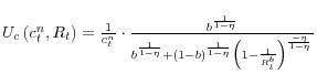
![\begin{displaymath} \frac{W}{P}\frac{1}{c}\left[ {\frac{b}{b+(1-b)\left( {\frac{b}{1-b}} \right)^{\frac{\eta }{\eta -1}}}} \right]=\frac{\psi }{1-l} \end{displaymath}](img188.gif)
The equilibrium will be characterized by a relation between real money balances and aggregate demand, the demand functions for capital and labor by each sector, the demand functions for the intermediate and sector goods, as well as price and wage rules. In a symmetric market equilibrium, all
firms within the labor intensive sector will make identical decisions about production, labor and capital inputs, as well as pricing. Thus in the symmetric equilibrium the subscripts ![]() and
and
![]() will be omitted from the optimal conditions. In addition, in equilibrium the desired real money balances equal actual money balances or
will be omitted from the optimal conditions. In addition, in equilibrium the desired real money balances equal actual money balances or
![]() . The symmetric equilibrium of the economy consists of an allocation
. The symmetric equilibrium of the economy consists of an allocation
![]() , and prices and wage
, and prices and wage
![]() such that given the values for
such that given the values for ![]() and
and
![]() the optimal conditions from the households', intermediate and representative firms' maximization problems are satisfied. All equations are shown in Appendix C.
the optimal conditions from the households', intermediate and representative firms' maximization problems are satisfied. All equations are shown in Appendix C.
6.3 The Effect of Nominal Disturbances in a Symmetric Market Equilibrium if Prices, Wages, and Rent are not allowed to Change (short-run equilibrium)
The following system of equations determines the immediate effect of an increase in nominal money balances when prices, wages and rent are unchanged and capital is fixed. The firms have a fixed amount of capital and the only way they can respond to the changes in quantity demanded is by changing
the amount of labor they hire. The households supply the labor at the pre-set wage. The system is similar to the system of equations characterizing the initial (long-run) equilibrium (shown in Appendix C), except for the equations that implicitly include the optimal prices, wages and rent chosen by
the firms and the households. For example - when not allowed to reset their prices or choose the amount of capital they rent - the intermediate firms in sector one have to figure out how much labor they need to hire in order to supply the new quantity demanded. The solution thus requires that
![]() for a firm in sector one and
for a firm in sector one and
![]() for a firm in sector two. By substituting
for a firm in sector two. By substituting ![]() with
with ![]() , the following system of equations can be used to determine the effect of an increase in the real money balances on
, the following system of equations can be used to determine the effect of an increase in the real money balances on
![]() , using the long-run equilibrium values for
, using the long-run equilibrium values for
![]() denoted by a bar.
denoted by a bar.
An increase in nominal balances, when prices of final output and factors of production remain constant, translates into an increase in the aggregate output produced - equation (59). From equations (55) and (56) it can be seen that the output in the two sectors increases proportionally. The production of output in each sector can increase by increasing the employed labor. The amount of capital each firm in the economy owns is predetermined, but labor is elastically supplied.
Again let sector one be labor-intensive and sector two be capital-intensive (i.e.
![]() . Then equations (57) and (58) imply that when there is an increase in nominal money balances, and prices in neither sector change, output in both sectors increases. This
result arises from the consumer preferences which map the change in the money supply into a change in consumption. Labor is more productive in the labor-intensive sector - as a result the labor employed there will increase by less than in the capital- intensive sector.
. Then equations (57) and (58) imply that when there is an increase in nominal money balances, and prices in neither sector change, output in both sectors increases. This
result arises from the consumer preferences which map the change in the money supply into a change in consumption. Labor is more productive in the labor-intensive sector - as a result the labor employed there will increase by less than in the capital- intensive sector.
6.4 The decisions of an atomistic firm in the labor-intensive and an atomistic firm in the capital-intensive sector when the aggregate price level, wages and rent have not yet changed in response to the nominal disturbance
The optimal pricing decisions for firm ![]() in the labor-intensive sector is derived again from the firm's optimization problem: the atomistic firm faces a new demand for its product but rent,
wages and aggregate price level are as in the long-run equilibrium.
in the labor-intensive sector is derived again from the firm's optimization problem: the atomistic firm faces a new demand for its product but rent,
wages and aggregate price level are as in the long-run equilibrium.
For example, firm ![]() in sector one solves:
in sector one solves:
![\begin{displaymath} \begin{array}{c} \mbox{Max }P_{1i} y_{1i} -(\overline R \,\overline k _{1i} +\overline W \,l_{1i} )\\ \ \par \mbox{s.t. }y_{1i} \le \overline k _{1i}^\alpha l_{1i}^{1-\alpha } \\ \ \par y_{1i} =\left[ {\frac{\overline P _1}{P_{1i} }} \right]^{\frac{1}{1-\theta}}y_1 \end{array}\end{displaymath}](img206.gif)
The new optimal price for a profit-maximizing firm (denoted by a superscript ![]() can be obtained:
can be obtained:
and
where
![]() are the respective marginal costs for sector one and two, which atomistic firms expect to face, given that wages, rents and other firms' prices remain unchanged. The new
optimal prices are again a mark-up, this time - over the marginal costs atomistic firms face immediately after the monetary policy shock.
are the respective marginal costs for sector one and two, which atomistic firms expect to face, given that wages, rents and other firms' prices remain unchanged. The new
optimal prices are again a mark-up, this time - over the marginal costs atomistic firms face immediately after the monetary policy shock.
Using the equalities:
![]() and
and
![y_{1i} =\left[ {\frac{\overline P _1}{P_{1i} }} \right]^{\frac{1}{1-\theta }}y_1](img212.gif) , the new optimal prices can be expressed as a function of the monetary policy shock:
, the new optimal prices can be expressed as a function of the monetary policy shock:
where
![]()
![]()
and
![]() for
for
![]() , which implies that firms re-setting prices in sector one will deviate less from the long-run equilibrium price level in response to both positive and negative monetary
policy shocks, i.e.
, which implies that firms re-setting prices in sector one will deviate less from the long-run equilibrium price level in response to both positive and negative monetary
policy shocks, i.e.
![]() .
.
This result arises due to the assumption that capital is fixed but labor is elastically supplied. In the case of an expansionary monetary policy shock, the marginal cost of production increases by more in the capital intensive sector, as they need to hire more labor in order to produce the new quantity demanded (labor is less productive in the capital-intensive sector). In the case of a negative monetary policy shock, the capital-intensive sector can release more labor and their marginal cost of production will decrease by more than in the labor-intensive sector.
6.5 Loss of profit from not adjusting when all other prices remain unchanged
Using the new optimal price ![]() (62) for a profit-maximizing firm in sector one, the new quantity the firm will be selling (
(62) for a profit-maximizing firm in sector one, the new quantity the firm will be selling (![]() and the profit for such firm (
and the profit for such firm (![]() can be obtained:
can be obtained:
![\begin{displaymath} \begin{array}{l} y_{1i}^m =\left[ {\frac{\overline P _1 }{P_{1i}^m }} \right]^{\frac{1}{1-\theta }}y_1 \\ \ \par V_{1i}^m =P_{1i}^m y_{1i}^m -TC_{1i}^m =P_{1i}^m y_{1i}^m -\overline R \overline k _{1i}-\overline W \overline k _{1i}^{\frac{-\alpha }{1-\alpha }} \left( {y_{1i}^m } \right)^{\frac{1}{1-\alpha }} \end{array}\end{displaymath}](img223.gif)
![]()
where
![C_1 =f(\alpha ,\theta ,\overline W ,\overline k _{1i},\overline P _1 )=\overline W \overline k _{1i}^{^{\frac{-\alpha }{1-\alpha }}} \left[ {\frac{1}{\theta }\frac{1}{1-\alpha }-1} \right]\left[ {\frac{1}{\theta }\frac{1}{1-\alpha }\frac{\overline W }{\overline P }\overline k _{1i}^{^{\frac{-\alpha }{1-\alpha }}} } \right]^{\frac{1}{1-\theta (1-\alpha )}}](img226.gif) is a constant.
is a constant.
A firm that does not adjust its price, in response to the nominal disturbance, sells all that is required from it at the preset price. Its profit after the change in the money supply is the following:
After a third order approximation, the opportunity cost (loss of profit) of not adjusting the price as a proportion of initial revenues is:
The loss function,
Correspondingly for a firm in sector two, the loss function is:
7. Menu Costs
Now let each firm face a fixed cost of adjusting its price (a menu cost) equal to a fraction of its initial total revenue. Firms will adjust their prices in response to the increase in nominal balances only if the gain from doing so outweighs the costs. In each sector there is a continuum of firms. Each firm within a sector faces a random fixed cost, which is drawn from a continuous distribution. Both sectors face the same distribution of menu costs. The assumption of a continuous distribution implies that in each sector there will be a marginal firm, which will be indifferent to changing its price. Within a sector, all firms that adjust their prices will choose the same new price, which will be different from the new price chosen by firms in the other sector.
In particular the fixed cost ![]() is i.i.d. across firms with c.d.f.
is i.i.d. across firms with c.d.f.
![]() and p.d.f.
and p.d.f.
![]() . I assume that
. I assume that
![]() for
for
![]() , thus the cost of adjusting the price is bounded.
, thus the cost of adjusting the price is bounded.
The adjustment decision for an individual firm depends on two factors: the loss of profit if the firm does not adjust and the realization of the fixed cost of adjustment, in this case both are specified as a fraction of the firms' initial revenues. For the marginal firm in sector one, the menu
cost will be equal to the loss of profit from not adjusting the price, and this firm will be indifferent to price adjustment:
From the distribution of the menu costs then we can determine the fraction of firms
For sector two the fraction of firms that adjust will be:
From equation (69) it follows that
8. The Short-run Equilibrium
The following analysis is to check whether more firms adjusting prices in the capital intensive sector - in response to a nominal disturbance - is an equilibrium. To do so, I will calculate the private gain to firms, expressed as a proportion of the initial (long-run
equilibrium) revenues, associated with the adjustment of its price in response to a change in nominal balances. If the difference in profits between the price-adjusting firms and the firms which keep their prices unchanged in the capital intensive sector is bigger than the corresponding difference
in the labor-intensive sector, then
![]() is indeed a short-run equilibrium. One possible reason - for
is indeed a short-run equilibrium. One possible reason - for
![]() not being an equilibrium - is for example a big change in the relative sectoral prices. If the change in the price level in sector two is so big that the demand for their
products decreases, the gain from changing prices by capital-intensive firms can turn out smaller compared to the gain realized by the price-adjusting firms in the labor-intensive sector.
not being an equilibrium - is for example a big change in the relative sectoral prices. If the change in the price level in sector two is so big that the demand for their
products decreases, the gain from changing prices by capital-intensive firms can turn out smaller compared to the gain realized by the price-adjusting firms in the labor-intensive sector.
If ![]() fraction of firms in sector one adjusts their prices to (64), the new price level in sector one will be:
fraction of firms in sector one adjusts their prices to (64), the new price level in sector one will be:
The aggregate price level will be:
Let
![A=\left[ {\mu _1 (1+\tilde {M})^{\frac{-\theta \,\Omega _1 }{1-\theta }}+1-\mu _1 } \right]^{-\frac{1-\theta }{\theta }}](img250.gif) and
and
![B=\left[ {\mu _2 (1+\tilde {M})^{\frac{-\theta \,\Omega _2 }{1-\theta }}+1-\mu _2 } \right]^{-\frac{1-\theta }{\theta }}](img251.gif) , so that
, so that
![]() and
and
![]() .
.
With the change in nominal balances and the change in aggregate price level in hand, I can calculate the new level of output that will be produced and consumed in the short-run equilibrium:
The last two equations show that the demand for a sector's product increases with the change in nominal balances (M), but is inversely related to the number of firms that are adjusting the prices in response to the change in M, and the size of the firms' price change.
With the change in the demand for sectoral output in hand, the new short-run equilibrium profit of price-adjusting producers in both sectors can be derived. The profit will be different from the expected profit the atomistic firm takes into account when choosing a new optimal price. The
difference is due to the fact that when atomistic firms take their decision, they assume that everyone keeps their price unchanged, which is no longer the case. The quantity a price-adjusting firm in the labor intensive sector (sector one) sells is:
Analogously in the capital-intensive sector:
and
Using the new prices and quantities, the short-run equilibrium profits for both price-adjusting and non-adjusting producers in sector one (labor-intensive sector) can be derived:
Using the equation describing the production function (
 , as well as equations (64), (82), and (83), the gain from adjusting prices in the
short-run equilibrium (i.e. after price have been adjusted) can be derived. In section 6.5 I argued that the loss of profit for the capital intensive producers from not adjusting their price is higher than the corresponding loss of profit for labor intensive producers and as a result the former
will be willing to pay higher menu costs to adjust prices. To check whether this response will be an equilibrium, I will check whether producers in the capital-intensive sector really gained more by adjusting their prices, now that a fraction of firms in each sector have changed their prices. Below
is an expression analogous to the private opportunity cost (
, as well as equations (64), (82), and (83), the gain from adjusting prices in the
short-run equilibrium (i.e. after price have been adjusted) can be derived. In section 6.5 I argued that the loss of profit for the capital intensive producers from not adjusting their price is higher than the corresponding loss of profit for labor intensive producers and as a result the former
will be willing to pay higher menu costs to adjust prices. To check whether this response will be an equilibrium, I will check whether producers in the capital-intensive sector really gained more by adjusting their prices, now that a fraction of firms in each sector have changed their prices. Below
is an expression analogous to the private opportunity cost (
In the labor-intensive sector, the profit of price-adjusting firms (as a fraction of the initial total revenue):
![\begin{displaymath} \frac{\Pi _{1i}^m }{\overline {TR} }=\left[ {\frac{A}{(1+\tilde {M})^{\Omega _1 }}} \right]^{\frac{\theta }{1-\theta }}(1+\tilde {M})-\theta (1-\alpha )\left[ {\frac{A}{(1+\tilde {M})^{\Omega _1 }}} \right]^{\frac{1}{(1-\theta )(1-\alpha )}}\left[ {\frac{A}{(1+\tilde {M})}} \right]^{\frac{-1}{(1-\alpha )}}-\frac{\overline R \overline k _{1i}}{\overline {TR} } \end{displaymath}](img266.gif)
The private gain to a labor-intensive producer - expressed as a proportion of initial revenues - associated with price adjustment in response to the change in the nominal balances is:
Analogously, for sector two:
It is very hard to compare analytically the private gains associated with price adjustments between the two sectors but the first derivative of the profit gain (
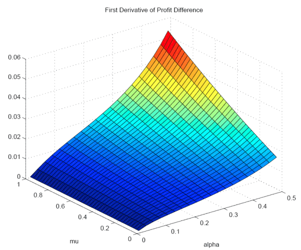
9. Data and Model Predictions
Going back to the original data on labor input share and frequency of price changes for the 29 SIC industries, one can split these industries into 2 sectors and compare the predictions of the model with data. The capital-intensive industries belong to the first sector, while labor-intensive ones form the second sector. Fourteen of the 29 industries fall into the first sector, whose cumulative weight is one half of all goods and services covered in the Bils and Klenow (2004) data. The weighted average share of labor input in the first sector is only 0.20 compared to 0.41 for the second (labor intensive) sector. The weighted mean frequency of price changes is 34.3% and 18.3% for the capital- and labor-intensive sectors respectively. Direct comparison of these numbers with the first model (no cost of price adjustment) predictions is not appropriate, since the data gives the frequency with which a sector changes price, while the model predicts the percentage change in nominal prices in response to a monetary policy shock. However, the amount by which a price changes in response to a monetary policy shock can be considered a good indicator of the probability with which a manufacturer will change the price of its product after the shock. For two sectors with equal weight a 1 percent increase in the growth rate of money generates: a 1.55 percent price increase in the nominal price for the capital-intensive sector (with share of labor input of 0.20), and a 1.23 percent price increase for the labor-intensive one (with share of labor input of 0.41). This means that doubling the labor input share (from 0.20 to 0.41) reduces the increase in the nominal price by 0.32 percentage point. It would be more interesting to compare the predictions of the menu cost model for the frequency of price changes across sectors, rather than the size of the price changes, and compare them with the data. As of this moment I leave this for future research.
That sectors differ in their responses to monetary shocks has already been shown in the paper by Ohanian, Stockman and Kilian (1995). They found that four of the eighteen SIC industries in their study (Food and Kindred Products, Lumber and Wood Products, Leather and Leather Products, and Primary Metals) show a more rapid price adjustment to a monetary shock than the aggregate for the economy. Consistent with the results shown here, three of these sectors have labor input shares whose values are significantly below the average of 0.31 (standard error 0.02) and the fourth has a labor share very close to the average. The Primary metals industry (not included in this study) has a labor input share of 0.23 according to the Jorgenson database.
It is also interesting to check whether the reverse relationship between labor share and frequency of price changes holds, i.e. to see if those industries which change their prices most often use relatively less labor in their production. To check this, I again split the 29 industries into two groups, only this time the division is based on the frequency of price changes criterion. Table 2 summarizes the main result, namely that the sector which changes prices more frequently, the "flexible price" sector, employs about half of the labor employed in the "sticky price" sector, and changes prices almost three times as often.
Table 3. Sticky vs. Flexible Price Sector
| Labor Share | Frequency of price change | |
|---|---|---|
| Sticky price sector | 0.39 | 13.84 |
| Flexible price sector | 0.23 | 37.69 |
10. Conclusion
Empirical evidence [Bils and Klenow (2004), Carlton (1986), Kashyap (1995), etc.] shows a wide range of price flexibility across commodities. The significant differences in the frequency of price changes across goods and sectors have motivated the search for possible sector and product characteristics that can explain the empirical findings in the context of new Keynesian models. At the same time, studies like Mankiw (1985) and Baxter (1996) have shown that monetary policy can have different effects on the various sectors of the economy. The objective of this paper is to assess the effects of nominal shocks on labor- and capital-intensive sectors in a model with staggered nominal wage contracts and ask whether such a model can account for certain features of the empirical evidence on price stickiness.
The first contribution of this paper is the finding that labor-intensive industries change prices of their products less often than capital-intensive industries do. This finding is based on micro-level pricing data published in the Bils and Klenow (2004) study. It motivated an investigation whether a standard staggered-wage model allowing for different labor and capital intensities across sectors can provide some insight on the effect of nominal disturbances and the frequency of price changes in various industries.
The analysis shows that in a sticky-wage model, real marginal costs in labor- and capital-intensive sectors respond differently to monetary shocks. An expansionary monetary policy shocks, for example, results in an increase in the real marginal cost for a capital-intensive industry and a decrease in the real marginal cost for a labor-intensive industry. Thus, a firm employing relatively more labor inputs, in an economy with rising inflation, faces a decrease in real marginal cost of production. The overall effect on its nominal price is smaller than the effect on a firm using relatively more capital. The difference in the responses of marginal costs can potentially provide insight as to why some firms change their prices frequently while others have sticky prices. However, labor intensity alone is not enough to produce price stickiness across sectors. Adding a menu cost of setting a new price is one solution to this problem. The second part of the paper shows that, in a one-period model with monopolistic competition, if two sectors face the same distribution of menu costs but differ in factor intensity, a smaller fraction of firms in the labor-intensive sector will pay the menu cost and will adjust their prices in response to a change in the nominal money balances. In the one-period model, because capital is fixed but labor is elastically supplied, an atomistic firm in the capital-intensive sector faces a bigger increase in the marginal cost and thus bigger losses from keeping its price unchanged. Assuming staggered wages does not change this result qualitatively but makes the result stronger.
Erceg (1997), Chari, Kehoe and McGratten (2000), and Huang and Liu (2002) have already shown that staggered wage models have the potential to generate persistent real effects of monetary shocks. The main finding of this paper is that staggered wage models with multiple sectors have the potential to account for the variety of price flexibility observed in the data.
Alavrez, L.J., P. Burriel, and I. Hernando (2005): "Price Setting Behaviour in Spain: Evidence from Micro PPI Data", ECB Working Paper Series No 522.
Barsky, R., C.L. House, and M. Kimball (2003): "Do Flexible Durable Goods Prices Undermine Sticky Price Models?" NBER working paper #9832.
Basu, S., and J. G. Fernald (1994): "Constant returns and small markups in U.S. manufacturing," International Finance Discussion Papers 483, Board of Governors of the Federal Reserve System.
Basu, S., and J. G. Fernald (1995): "Aggregate Productivity and the Productivity of Aggregates," NBER working paper #5382.
Baxter, M. (1996): "Are Consumer Durables Important for Business Cycles?," The Review of Economics and Statistics, MIT Press, vol. 78(1), pages 147-55.
Bils, M., and P.J. Klenow (2004): "Some Evidence on the Importance of Sticky Prices,"
Journal of Political Economy, 112(5), 947-985.
Bils, M., P.J. Klenow, and O. Kryvtsov (2003): "Sticky Prices and Monetary Policy Shocks," The Quarterly Review, Federal Reserve Bank of Minneapolis 27(1), 2-9.
Blanchard, J., and N. Kiyotaki (1987): "Monopolistic Competition and the Effect of Aggregate Demand," The American Economic Review, 77(4), 647-666.
Blinder, A., and G.N. Mankiw (1984): "Aggregation and Stabilization Policy in a Multi-Contract Economy," Journal of Monetary Economics, 13(1), 67-86.
Card, D., and D. Hyslop (1997): "Does Inflation "grease the wheels of the labor market"?" in Reducing Inflation, ed. by C. Romer and D. Romer, pp. 71-114. University of Chicago Press, Chicago.
Calvo, G.A. (1983): "Staggered Prices in a Utility Maximizing Framework," Journal of Monetary Economics, 12(3), 383-398.
Carlton, D.W. (1986): "The Rigidity of Prices," American Economic Review, 76(4), 637-658.
Caucutt, E.M., M. Ghosh, and C.M. Kelton (1999): "Durability versus Concentration as an Explanation for Price Flexibility," Review of Industrial Organization, 14(1), 27-50.
Cecchetti, S. G. (1987): "Indexation and incomes Policy: a Study of Wage Adjustment in Unionized Manufacturing," Journal of Labor Economics, 5(3), 391-412.
Cecchetti, S. G. (1986): "The Frequency of Price Adjustment: a Study of Newsstand Prices of Magazines," Journal of Econometrics, 31(3), 255-274.
Chari, V.V., P. J. Kehoe, and E.R. McGratten (2000): "Sticky Price Models of the Business Cycle: Can the Contract Multiplier Solve the Persistence Problem?" Econometrica, 68(5), 1151-1179.
Cho, J.O., and T.F. Cooley (1995): "The Business Cycle with Nominal Contracts," Economic Theory, 6(1), 13-33.
Christiano, L.J., M. Eichenbaum, and C.L. Evans (2005): "Nominal Rigidities and the Dynamic Effects of a Shock to Monetary Policy," Journal of Political Economy, 113(1), 1-45.
Davis, M., and J.D. Hamilton (2004): "Why Are Prices Sticky? The Dynamics of Wholesale Gasoline Prices," Journal of Money, Credit and Banking, 36(1), 17-37.
Dixit, A. K., and J.E. Stiglitz (1977): "Monopolistic Competition and Optimal Product Diversity," American Economic Review, 67(3), 298-308.
Dutta, S., M. Bergen, and D. Levy (2002): "Price Flexibility in Channels of Distribution: Evidence from Scanner Data," Journal of Economic Dynamics and Control, 26, 1845-1900.
Erceg, C.J. (1997): "Nominal Wage Rigidities and the Propagation of Monetary Disturbances," Federal Reserve Board International Finance Discussion Paper #590.
Erceg, C.J., and A.T. Levin (2006): "Optimal Monetary Policy with Durable Consumption Goods," Journal of Monetary Economics, 53, 1341-1359.
Griffin, P. (1992): "The Impact of Affirmative Action on Labor Demand: a Test of Some Implications of the Le Chatelier Principle," Review of Economics and Statistics, 74, 251-260.
Griffin, P. (1996): "Input Demand Elasticities for Heterogenous Labor: Firm-level Estimates and an Investigation into the Effects of Aggregation," Southern Economic Journal, 62, 889-901.
Jorgenson, D. W. and K. J. Stiroh (2000): "Raising the Speed Limit: U.S. Economic Growth in the Information Age," Brookings Papers on Economic Activity, 1, 125-211
Huang, K.X.D., and Z. Liu (2002): "Staggered price-setting, staggered wage-setting, and business cycle persistence," Journal of Monetary Economics, 49(2), 405-433.
Ireland, P. N. (2004): "Technology Shocks in the New Keynesian Model," The Review of Economics and Statistics, 86(4), 923-9363.
Kashyap, A. K. (1995): "Sticky Prices: New Evidence from Retail Catalogs," The Quarterly Journal of Economics, 110(1), 245-274.
Kiley, M. T. (2002): "Partial Adjustment and Staggered Price Setting," Journal of Money, Credit and Banking, 28(2), 283-298.
MacDonald, J. N., and D. Aaronson (2001): "How Do Retail Prices React to Minimum Wage Increases," Federal Reserve Bank of Chicago Working Papers Series, WP 2000-20.
Mankiw, N. G. (1985): "Small Menu Costs and Large Business Cycles: A Macroeconomic Model of Monopoly," Quarterly Journal of Economics, 100, 529-537
Mankiw, N. G., and R. Reis (2002): "Sticky Information Versus Sticky Prices: A Proposal to Replace the New Keynesian Curve," Quarterly Journal of Economics, 117, 1295-1328
Nakamura, E., and J. Steinsson (2008): "Five Facts About Prices: A Reevaluation of Menu Costs Models," Quarterly Journal of Economics, 123(4), 1415-1464.
Ohanian, L., A. Stockman, and L. Kilian (1995): "The Effects of Real and Monetary
Shocks in a Business Cycle Model with Some Sticky Prices," Journal of Money, Credit and Banking, 27(4), 1209-1234.
Olivei, T., and S. Tenreyro (2004): "The Timing of Monetary Policy Shocks," FRB Boston Working Papers Series, 04-1.
Schmitt-Grohe, S., and M. Uribe (2004): "Optimal Simple and Implementable Monetary
and Fiscal Rules," NBER working paper #10253.
Sims, C.A. (2001): "Solving Linear Rational Expectations Models," Journal of Computational Economics, 20, 1-20.
Taylor, J.B. (1980): "Aggregate Dynamics and Staggered Contracts," Journal of Political Economy, 88(1), 1-23.
Taylor, J.B. (1983): "Union Wage Settlements During a Disinflation," American Economic Review, 73(5), 981-993
Taylor, J.B. (1993): "Macroeconomic Policy in the World Economy: from Econometric Design to Practical Operation," W.W. Norton, New York
Taylor, J.B. (1999): "Staggered Price and Wage Setting in Macroeconomics," in Handbook of Macroeconomics, ed. by J. Taylor and M. Woodford, vol.1B, pp. 1009-1044. Elsevier Science B.V.
Appendix A: Data on Monthly Frequency of Price Changes
Table 4. Data for 29 SIC Industries by Category
| # Name | Weighted Average Monthly Frequency of Price Changes 1995-1997 |
Average Share of
Labor Inputs in Total Output 1958-1996 |
Number of ELI in each Industry | Industry weight in 1995 CEX |
|---|---|---|---|---|
| 1 Agriculture | 37.92% | 0.26 | 12 | 1.60 |
| 7 Food and kindred products | 31.53 | 0.16 | 85 | 9.42 |
| 8 Tobacco | 21.25 | 0.15 | 3 | 0.87 |
| 9 Textile mill products | 14.97 | 0.23 | 5 | 0.20 |
| 10 Apparel | 33.47 | 0.33 | 44 | 4.15 |
| 11 Lumber and wood | 21.60 | 0.25 | 1 | 0.01 |
| 12 Furniture and fixtures | 23.01 | 0.36 | 9 | 1.19 |
| 13 Paper and allied | 17.64 | 0.26 | 2 | 0.43 |
| 14 Printing, publishing and allied | 8.28 | 0.40 | 7 | 0.73 |
| 15 Chemicals | 15.05 | 0.24 | 13 | 2.26 |
| 16 Petroleum and coal products | 72.18 | 0.09 | 10 | 3.48 |
| 17 Rubber and misc. plastics | 29.91 | 0.32 | 3 | 0.30 |
| 18 Leather | 25.85 | 0.33 | 5 | 1.02 |
| 19 Stone, clay, glass | 15.93 | 0.37 | 6 | 0.13 |
| 21 Fabricated metal | 12.38 | 0.35 | 3 | 0.12 |
| 22 Machinery, non-electrical | 29.72 | 0.36 | 10 | 0.84 |
| 23 Electrical machinery | 26.26 | 0.35 | 18 | 1.34 |
| 24 Motor vehicles | 37.12 | 0.19 | 4 | 5.04 |
| 25 Transportation equipment & ordnance | 18.96 | 0.43 | 3 | 0.28 |
| 26 Instruments | 10.85 | 0.46 | 9 | 0.55 |
| 27 Misc. manufacturing | 17.38 | 0.33 | 12 | 1.75 |
| 28 Transportation | 27.96 | 0.41 | 10 | 2.55 |
| 29 Communications | 13.37 | 0.32 | 4 | 3.23 |
| 30 Electric utilities | 43.40 | 0.21 | 1 | 2.88 |
| 31 Gas utilities | 64.20 | 0.11 | 1 | 1.01 |
| 32 Trade | 8.86 | 0.50 | 7 | 5.39 |
| 33 Finance Insurance and Real Estate | 17.21 | 0.28 | 5 | 3.09 |
| 34 Services | 14.97 | 0.43 | 54 | 14.75 |
| 35 Government enterprises | 3.79 | 0.38 | 4 | 0.35 |
| Weighted average for the economy: | 26.1 | 0.31 | Total: 68.94 |
Appendix B: A System of log-linearized equations defining the DSGE model equilibrium
To analyze how the economy responds to monetary policy shocks, I will need to approximate the system of non-linear equations, defining the equilibrium, by a system of linear equations that characterize the dynamics of the model for small deviations around the non-stochastic steady state. A first
order Taylor approximation around the stationary steady state will produce equations that are linear in the log-deviations of the variables. The variables in these equations will be expressed as percentage deviations around the steady state. The percentage deviation of variable![]() , around its steady-state value
, around its steady-state value![]() , will be denoted by
, will be denoted by![]() , where
, where
![]() .
.
The following real variables have been obtained by normalizing their nominal equivalents using the aggregate price level![]() :
:
![]() ,
,
![]() ,
,
![]() ,
,
![]() and the following equations contain only logarithmic deviations of real variables from their steady-state values:
and the following equations contain only logarithmic deviations of real variables from their steady-state values:
Equations (1B) - (3B) are the log-linearized versions of the production technology and the input demand functions for the firm producing the final good, or equations (1), (3), and (4) in the main text.
(1B)
![]()
(2B)
![]()
(3B)
![]()
Equations (4B) and (5B) are derived by log-linearizing the production functions in sectors one and two, or equations (12) and (13) in the paper. Also, after log-linearizng the demand functions for labor and capital by the intermediary firms from the two sectors (18)-(21), equations (6B) - (9B) can be obtained.
(4B)
![]()
(5B)
![]()
(6B)
![]()
(7B)
![]()
(8B)
![]()
(9B)
![]()
The following two equations, (10B) and (11B), can be derived directly from the households' demand for real money balances and the Euler equation for consumption, after substituting the expression for marginal utility of consumption.
(10B)
![]()
(11B)
![]()
Using the fact that in steady state there is no inflation (i.e.
![]() and the real rate of return on capital satisfies:
and the real rate of return on capital satisfies:
![]() , the log-linearization of the expression for the supply of capital by households (39), yields the following equation:
, the log-linearization of the expression for the supply of capital by households (39), yields the following equation:
(12B)
![]()
The additional first order condition for households in a wage-setting cohort (41) was used to obtain (13B).
(13B)
![]()
The following two equations, (14B) and (15B), are the log-linearized versions of the demand for households' labor (43) and (44) in the main text. Equation (16B) can be obtained directly form (42), after substituting the nominal wage chosen by each cohort with its real equivalent to obtain the real aggregate wage rate.
(14B)
![]() for
for
![]()
(15B)
![]() for
for
![]()
(16B)
![]()
After the log-linearization of the three market clearing condition (27), (28), and (48), equations (17B) - (19B) are obtained.
(17B)
![]()
(18B)
![]()
(19B)
![]()
Using the expression for real money balances
![]() and substituting for nominal money balances, equations (45) and (46) yield (20B) and (21B).
and substituting for nominal money balances, equations (45) and (46) yield (20B) and (21B).
(20B)
![]()
(21B)
![]()
In addition (22B) and (23B) show the log-linearized expressions for the real marginal cost in sector one (49) and sector two (50), respectively.
(22B)
![]()
(23B)
![]()
In the above system of log-linearized equations:
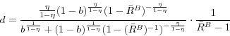
Appendix C: System of Equations Characterizing The Long-Run Market Equilibrium In A One-Period Economy With Menu Costs
From the final good production problem:
(C1)
![]()
(C2)
![]()
(C3)
![]()
From the intermediate firms' problems
(C4)
![]()
(C5)
![]()
(C6)
![]()
(C7)
![]()
(C8)
![]()
(C9)
![]()
From the household's decisions:
(C10)
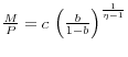
(C11)
![\frac{W}{P}\frac{1}{c}\left[ {\frac{b}{b+(1-b)\left( {\frac{b}{1-b}} \right)^{\frac{\eta }{\eta -1}}}} \right]=\frac{\psi }{1-l}](img321.gif)
Market clearing conditions require:
(C12) ![]()
(C13) ![]()
(C14) ![]()