A Study of U.S. Monetary Policy Implementation: Demand for Reserves on a Period Average Basis
Keywords: Monetary policy implementation, reserve demand
Abstract:
JEL Codes: E5, E52, E58
As central banks around the world move to systems that rely more on the demand for excess reserve balances or some form of voluntary reserve holdings rather than on required reserves (Clouse and Dow, 2002), it is instructive to examine closely the demand for period average excess reserve balances in the U.S. system. The results in this paper provide insight into one of the tools used to guide staff in the provision of reserve balances throughout the maintenance period. While this is surely not the only tool used to forecast demand, this paper shows that there exist some consistencies in the demand for reserve balances over the maintenance period that are not at odds with previous theoretical work.2
The Federal Reserve implements conventional monetary policy by conducting open market operations to align the supply of balances held by depository institutions (DIs) at Federal Reserve Banks with demand for those balances so that federal funds trade around the target rate set by the Federal Open Market Committee (FOMC). Aside from open market operations, the supply of balances is determined largely by so-called autonomous factors, including the Treasury's balance at the Federal Reserve, currency in circulation, and check float. The demand for balances can vary significantly from day to day. Staff at the open market operations desk at the Federal Reserve Bank of New York (the Desk) and at the Federal Reserve Board (the Board) estimate the expected demand for balances at the policy target each day. The daily estimates take into account market conditions, including expectations of high payment flows, the day of the two-week maintenance period, and information gathered from discussions with banks and brokers.
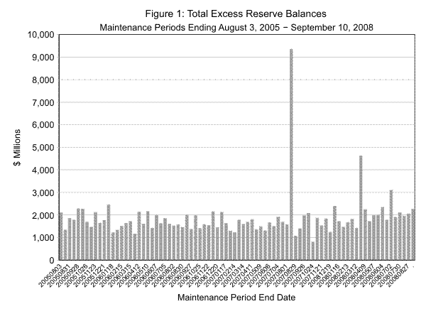
Most of the analysis of the demand for reserve balances is focused on the demand for excess balances, which are balances held over and above reserve balance requirements. Board and Desk forecasters formulate their excess reserve balance demand forecasts on a daily basis as well as for the two-week maintenance period as a whole. In particular, Board and FRBNY staff estimate the volume of excess balances that will be demanded on a maintenance-period average basis, known as period average excess, or PAE. Figure 1 displays PAE over the period from August 2005 through September 2008. In general, PAE ranges from about $1 billion to $2 billion. However, as can be seen in the figure, there are two clear outliers: the maintenance period ended August 15, 2007, which included the week in the turmoil began; and the maintenance period ended March 26, 2008, which included the collapse of Bear Stearns.3 Over the two years from August 3, 2005 to August 5, 2007, PAE averaged $1.7 billion but varied substantially, ranging from $1.2 billion to $2.4 billion. Over the year of market turmoil that began in earnest in August, 2007, PAE averaged $1.8 billion, ranging from $800 million to $3.1 billion.4
There is a long and extensive theoretical literature discussing reserves management and the demand for excess reserve balances. Poole (1968), who developed one of the early models of reserve management, showed that much of the demand for balances was related to uncertainty in the level of balances held in Fed accounts. Other researchers, including Clouse and Dow (1999, 2002), extended these ideas, and showed that the cost of discount window borrowing and the carryover provision (to be explained more fully later) also were key drivers of reserve demand.
Fewer papers explore the empirical evidence of demand for excess reserve balances, although there are selected key exceptions. Evanoff (1989) provides estimates using bank-level data from the Seventh Federal Reserve District that suggest banks respond to various institutional features of reserve management in ways that one would expect from theory. More recently, Bartolini et al. (2001) empirically document some of the salient features of reserve demand presented in this paper; however, their focus is on developing a theoretical model that explains the stylized facts, rather than on estimating parameters of a function describing the demand for excess balances.
This paper empirically explores the demand for excess reserve balances on a period average basis. Our analysis differs from previous research in two major ways. First, we find that it is crucial to take into account institution size and charter type when formulating period average excess forecasts. As we will illustrate extensively throughout the paper, large DIs tend to manage their excess reserve balances very carefully and tend to end the period with minimal excess while small DIs generally hold a buffer stock of excess that varies relatively little either within the maintenance period or across maintenance periods. Earlier studies of reserve demand either ignore, or, due to data limitations, do not explicitly consider demand for reserve balances by institution size or type. We show that the behavior of the large DIs differs substantially from that of others.
Second, and perhaps more importantly, the data discussed in this paper and used in the estimates we present are some of the real-time inputs that have been used by Board staff in formulating their forecasts for the demand for excess balances at the Federal Reserve. However, it should be noted that the parameters are re-estimated through time and the results are only one of the various tools used for analysis supporting open market operations. 5 We formulate our forecasts for PAE at three points in the maintenance period: before the period begins, a little more than halfway through the period, and at the start of the last three days of the period. Using a two-year sample that covers only the period prior to the beginning of the market turmoil in August 2007, we find that the ex-ante method with the lowest variance has a mean absolute error of about $160 million. Our mid-period forecast, with a mean absolute error of about $120 million, is an improvement over the ex-ante forecast, due to incoming information. The forecast formulated on the morning of the twelfth day of the period has the best performance overall, with a mean absolute error of just $80 million, considerably smaller than other rules-of-thumb. When our models are extended to include the year from August 2007 to September 2008, the forecast errors are larger, consistent with the increased uncertainty and volatility of this period: Our ex-ante forecast has a mean absolute error of about $180 million; our mid-period forecast error is $140 million, and our late-period forecast error is $110 million.
It should be noted at the outset that we do not use prices anywhere in our models; our formulations are in terms of quantities of reserve balances.6 However,
it should be noted that over the earlier part of the sample, funds traded slightly less than one basis point above the target on average, with an absolute mean average deviation from the target of about 3
![]() basis points, which provides support for our (implicit) assumption that our estimates are conditional
on a funds rate at the target. Over the market turmoil period, funds traded funds traded slightly less than 3 basis points above the target on average, with an absolute mean average deviation from the target of about 9 basis points. As a result, the implicit assumption of funds trading at the
target seems reasonable, and the model does a fairly good job at forecasting period average excess balances.
basis points, which provides support for our (implicit) assumption that our estimates are conditional
on a funds rate at the target. Over the market turmoil period, funds traded funds traded slightly less than 3 basis points above the target on average, with an absolute mean average deviation from the target of about 9 basis points. As a result, the implicit assumption of funds trading at the
target seems reasonable, and the model does a fairly good job at forecasting period average excess balances.
The remainder of the paper proceeds as follows. Section 1 reviews background on the supply and demand framework for Fed balances, the primary features of monetary policy implementation, and the data used in this paper. Section 2 presents our analytical framework and estimation results for the three forecasts, and includes the Board's ultimate technique to estimate reserves. Section 3 discusses comparative forecast performance. Section 4 concludes.
Background
In order to provide perspective for the empirical results, the next three subsections review the supply and demand framework for Fed balances, provide a closer look at the components of the demand for Fed balances, and describe the data used in the analysis.
A framework for the supply and demand for Fed balances
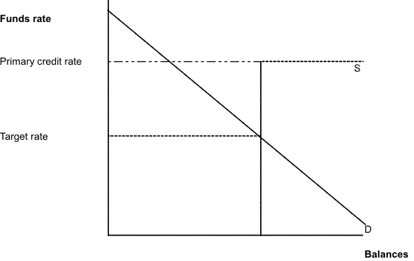
The illustration below summarizes a stylized supply and demand framework for Fed balances. The (inverse) demand curve for reserve balances slopes down, as demand for balances is assumed to increase with decreases in the federal funds rate. Indeed, previous research shows that the demand curve usually does slope down; this "liquidity effect" has been identified in the data at both a daily and a monthly frequency.7
The supply of reserve balances is determined largely by the Federal Reserve's portfolio of securities and repurchase agreements, discount window borrowing, and other items on the Fed's balance sheet, also known as "autonomous factors."8 Board and Desk staff produce forecasts each morning for the major autonomous factors, including the Treasury's balance at the Fed, the change in currency in circulation, and check float. Thus, the supply curve is vertical up to a rate equal to the primary credit rate. It is then horizontal at the primary credit rate, as banks obtain discount window loans when market conditions are tight, increasing the total supply of Fed balances (S). 9
As discussed in the introduction, the Federal Reserve implements monetary policy by conducting open market operations to align the supply of balances held by depository institutions (DIs) at Reserve Banks with demand for those balances so that federal funds trade around the target rate set by the Federal Open Market Committee (FOMC). By buying securities, either temporarily or outright, the Desk can add balances to the system and move the supply curve to the right; alternatively, the Desk can sell securities and drain balances from the system in order for the supply curve to intersect the demand curve at the target federal funds rate.
A closer look at the demand for Fed balances
As this paper concentrates on the demand for Fed balances, it is instructive to examine this demand a bit more closely. Demand for reserve balances held at the Federal Reserve can be divided into three parts. First, required reserve balances are those that DIs need to hold to meet their reserve requirements. Required reserves may be held in vault cash or in reserve balances; thus, required reserve balances are the difference between required reserves and vault cash. Second, contractual clearing balances are balances that DIs agree in advance to hold; they are generally held to cover clearing needs. Third, excess balances are those demanded over and above requirements. DIs typically hold excess balances on a precautionary basis in light of uncertain flows in and out of their reserve accounts. The sum of required reserve balances and contractual clearing balances, less as-of adjustments, is known as required operating balances, or ROB.10 The middle panel (b) of table 1 provides summary statistics on required operating balances by entity type. Of the $14.8 billion in ROB, a few dozen of the largest banks, the large money center banks (LMCBs) account for almost half the funds. The next largest share of ROB is held by small commercial banks (SCBKs), which hold about 20 percent, with other large commercial banks (OLCBs), thrifts (THINs), foreign institutions (FORIs), and nonreporting institutions (NONR) hold the remaining 30 percent.11
Excess reserve balances are held voluntarily by DIs, typically as a cushion to guard against overdrafts. Excess balances are calculated as the difference between balances held at the Federal Reserve and ROB. Holding balances in excess of required operating balances helps DIs to avoid overdrafts but carries opportunity costs. In contrast, closely managing excess reserve balances in order to minimize excess holdings while still avoiding overdrafts entails costs associated with staffing reserves management activities. As a general proposition, for larger banks, the benefits of managing excess balances closely frequently outweigh the costs, while for smaller institutions the costs generally appear to outweigh the benefits.
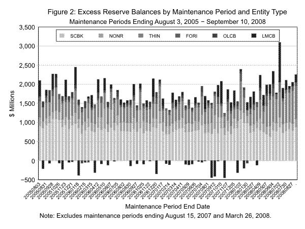
As evidence of this proposition, figure 2 displays PAE by type of depository institution for each of the maintenance periods ending August 3, 2005 through September 10, 2008. As is clear from the figure, roughly half of the excess balances are held by SCBKs; this share is relatively stable across periods. By contrast, the shares held by the LMCBs and OLCBs are small, but highly variable.
The middle panel (b) of table 1 summarizes the data presented in figure 2 and provides additional summary statistics by entity type. LMCBs have the lowest average PAE but the highest standard deviation of all entity types. In contrast, SCBKs hold about half of PAE, which, as measured by the coefficient of variation, appears to fluctuate relatively little.
Indeed, as seen in the bottom panel (c) of Table 1, LMCBs hold little excess on average compared to their substantially larger ROB. By contrast, SCBKs and THINs tend to hold more excess, both in levels and proportionally. NONRs face low ROB, but have the highest ratio of excess to ROB of any entity type. Overall, these statistics indicate that large and small institutions manage their excess quite differently.
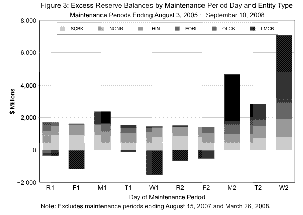
In addition, it is notable that excess reserve balances vary considerably from day to day. Figure 3 shows average excess balances by day of the period and by entity type. Reserve maintenance periods cover two weeks, beginning on a Thursday (R1) and ending on a Wednesday (W2). The last three days of the period thus fall on Monday, Tuesday, and Wednesday. Excess balances are generally highest on the last few days of the period, and the greatest variation is seen in the holdings of LMCBs. Both LMCBs and FORIs tend to increase their holdings of excess balances considerably over the last three days of the period. However, as noted in Table 1, both of these entity types hold relatively little excess on a period average basis. The final three days of the period are thus crucial because the bulk of excess is typically held then.
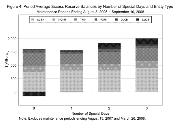
With these facts in mind, the first step in our analysis is to identify the factors that appear to affect PAE. First, ongoing observation indicates that demand for balances increases as the volume of payments increases, typically following holidays, at month-turn, and at mid-month, days known collectively as high payment flow days. On such days, DIs likely face greater uncertainty about their end-of-day balances and thus have a greater incentive to hold excess balances as a precaution against overdrafts. The greater the number of such days in a period, the higher PAE is likely to be. The number of high payment flow days varies from maintenance period to maintenance period according to the calendar configuration. Figure 4 presents averages of PAE grouped by the number of high payment flow days in the period. Generally, PAE is higher in periods with more high payment flow days.12
A second factor we consider likely to affect excess balances is carry-over, a provision that allows DIs to carry over some excess or deficiency of their required reserve balances in a reserve maintenance period to be used or made up in the next maintenance period.13 This feature provides DIs with flexibility in meeting their reserve balance requirements and allows some smoothing of demand for balances, with the likely effect of reducing volatility of the overnight federal funds rate.
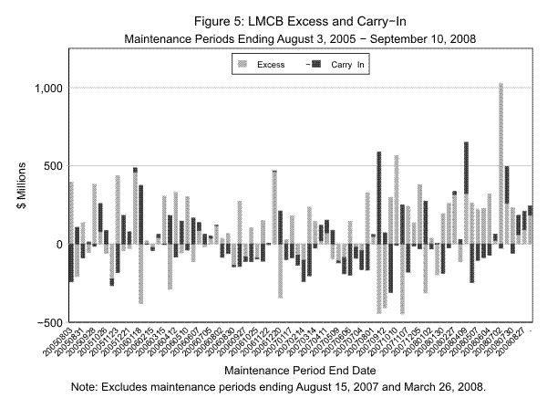
Since larger DIs tend to more actively manage their reserve balances than smaller institutions, their demand for excess balances tends to be fairly sensitive to carry-over. In principle, the use of carry-over by large DIs should be affected by conditions in the federal funds market.14 If reserve market conditions are particularly tight on the last day of the maintenance period, large DIs might be expected to allocate part of their reserve needs to the following maintenance period, and vice versa. In turn, this use of carryover might affect the demand for excess in the current period. Indeed, as noted above, LMCBs manage their excess balances, including carry-over, to levels near zero. As a result, LMCB period average excess, while small, is sensitive to LMCB carry-in. As shown in figure 5, in more than half of the maintenance periods in our sample, carry-in and LMCB excess balances are of opposite sign, and often of similar magnitude. Consistent with this observation, the correlation between carry-over and LMCB excess is about -0.35 over the sample.
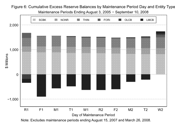
Figure 6, the cumulative analog of Figure 3, displays cumulative average excess to date by entity type and day of the maintenance period and illustrates a rule-of-thumb forecast of period average excess using information available after the second Friday of the maintenance period. The far right bar, which indicates cumulative excess for settlement day (W2), is also period average excess by entity type. For all entity types except LMCBs, PAE is quite similar to the level of cumulative excess on the second Friday. Moreover, LMCBs usually satisfy the bulk of their requirements on the last few days of the period. LMCBs are typically deficient on the second Friday but end the period with minimal excess in carry-in adjusted terms. Notably, DIs, including LMCBs, sometimes satisfy their balance requirements well in advance of the end of the period, causing them to be "locked in" to a positive excess position for the remainder of the period. The data show that, after accounting for carry-in and lockins, period average excess at LMCBs tends to be minimal.
Finally, one might expect that the level of ROB could affect PAE if DIs see a need for a minimum level of balances to meet clearing needs. Indeed, the Desk (2006, p. 6) notes that "experience suggests that there is some level of aggregate balances necessary to maintain liquidity in the reserves market", suggesting that if ROB were to drop to very low levels, banks might demand higher levels of excess in order to meet that minimum level.
Data flows
The stylized facts presented guide the regression analysis discussed in the next section. However, because forecasting demand for Fed balances is done every morning under very tight deadlines, it is instructive to review the data sources used for this purpose and the nature of these data sources compared to other data available on bank reserves in order to understand the tools available for forecasting demand for excess reserve balances.
The process actually begins the night before, when banks settle their positions for the evening with the Federal Reserve. These end-of-day positions are then aggregated by entity type (LMCB, OLCB, SCBK, THIN, FORI, and NONR) in order to determine the amount of excess, quantity of overdrafts, and level of discount window and other borrowing by each entity type. Once they are aggregated, they are transmitted to the Board and Desk forecasting staffs for use the following morning.
In addition, the positions of selected large institutions are reported on a disaggregated basis to the Federal Reserve Bank of New York. These positions are then transmitted to the forecasting staffs. These data can indicate unusual movements in reserves holdings at the largest DIs and allow us to identify carry-over.
The items on these data flows determine part of the information set available for forecasting demand for fed balances each morning. Notably, these are real-time data flows. The main difference between these data flows and those available at later dates is the application of as-ofs - although some of these as-of are known by DIs in real time, others are not. An as-of adjustment is a memorandum item that the Federal Reserve applies to a depository institution's position to offset the effect of certain types of errors made to their position or to pay for float attributable to that institution. Importantly, an as-of adjustment does not affect intraday balances held in a reserve account, but does affect the bank's cumulative reserve position. As-ofs can be applied to maintenance periods in the past, present, or future. Since the data used in this study are real-time, the changes in cumulative position resulting from the application of an as-of to the current period at a later date would not be used in the estimation results here. In rare cases, an as-of adjustment is applied to the current maintenance period; in a subset of these cases, the DI would know about an as-of adjustment before it would appear in the data. However, these cases are very rare. In general, if an as-of adjustment has not yet been applied in the current period, it will not be applied until after the period ends and thus the data are in line with the DI's real-time understanding of its position. This distinction is important because it allows us to study bank behavior with the positions they thought they held at the time, not those that they were later revealed to have.
The data flows available to Board staff each morning also dictate the frequency and the structure used for forecasting period average excess. In our exercise, we forecast demand at three points in the maintenance period. The first forecast point is before the period begins or, practically speaking, on the morning of the second day of the period. Available data at that point include LMCB carry-in and the number and configuration of special days in the period. Operationally, Board and Desk staff tend to keep this initial PAE figure in mind as they formulate their forecasts for the demand for excess on each day of the period.
The second forecast point we employ in our modeling process is the morning of the ninth day of the period, when data through the second Thursday are available. At this point, Board staff start to focus more closely on the period demands for excess as well as the individual day demands. We conjecture that larger DIs, who tend to manage their excess closely, also start to concentrate more on their period needs around this point.
We base our final model forecast on data available on the morning of the second Monday of the period. With only three trading days and about 20 percent of the period left, much is already known about reserve market conditions and the demand for balances so far in the period. However, as shown in figure 3, many banks satisfy their demand for excess and their requirements on these last three days. Demand for the period clearly can rely critically on the demand over these last three days.
Analytical frameworks and estimation results
The stylized facts presented above guide our specifications for the regression analysis. The next section develops the analytical frameworks used for each of the three forecasting exercises and presents estimation results for each specification.
Ex ante forecast
Our ex ante forecasts have a relatively parsimonious specification, partly because the data limitations are most severe at that point. In line with the stylized facts presented above, we use the number of high payment flow days and carryover as explanatory factors for PAE, keeping in mind the
fact that most of the variability in excess is due to the LMCBs. We also include a supply-side influence on excess balances, the forecast miss attributable to market factors on the last day of the maintenance period. In contrast to earlier days in the maintenance period, when DIs and the Desk have
the opportunity to adjust their excess position and excess provision on subsequent days, a forecast miss on the last day of the period could have a significant impact on observed PAE. To the extent that a large settlement-day forecast miss moves PAE in a given maintenance period, we would want to
account for its effect separately from the Desk's decisions.15 With these thoughts in mind, our ex ante specification is
where PAE is the forecasted period average excess for all entity types (total period average excess), Sumhpf is the number of high payment flow days in the period, LMCBCarryin is LMCB carry-in, ROB is the level of required operating balances, and E(miss) is the expected factors forecast miss on the last day of the period. As for notation,
Table 2 displays our results. Note that ROB does not appear in these regression results. Preliminary regressions, not shown, indicated that ROB is not significantly correlated with total excess, and that the correlations between excess and ROB are of marginal significance and the sign varies by entity type. In addition, we estimated the same set of regressions for the earlier sample; results were qualitatively and quantitatively similar. The first column shows our results using total excess. In line with the data shown in figure 4, for each high payment flow day in the period, PAE increases by about $150 million. In a hypothetical period without high payment flow days and with no carry-in, PAE would be roughly $1.5 billion. However, almost all maintenance periods have at least one high payment flow day, pushing PAE up to between $1.6 billion and $1.7 billion.16 Consistent with the data presented in figure 5, higher carry-in is strongly associated with lower excess and the null hypothesis that the coefficient is -1 cannot be rejected. Finally, the forecast error on the final day of the period is significantly positively correlated with final excess, which is not a surprising result.17
Turning to the results by entity type, for LMCBs, the level of carry-in and the forecast error on the last day of the maintenance period are significantly correlated with excess. Notably, the hypothesis that the constant is equal to zero cannot be rejected, confirming our impression that LMCBs typically manage their excess to zero. In contrast, for all of the remaining entity types, we can easily reject this hypothesis. The number of high payment flow days is a significant predictor of PAE for a majority of the remaining entity types, consistent with DIs' increased incentive desire to hold excess reserves as a buffer against potential overdrafts on these days.
Day 9 and Day 12 Forecasts
Having developed an ex-ante regression-based forecasting method, we explored approaches to forecasting PAE towards the end of the period, when more information is available and when forecasts for the appropriate daily excess target are more closely tied to expected period average excess. To this
end, we specify regression models that accounts for two sets of factors, one set based on the cumulative positions of each depository institution entity type and one set based on the calendar-related features of the period. Our preliminary specification is

where E(type) corresponds to our expected period average excess by entity type at that point in the period. (Period average excess is denoted by
- LMCBs manage excess to zero, except for lockins and carryin;
- OLCBs manage excess to zero, except for lockins;
- SCBKs hold the same level of excess on each day of the period;
- Large THIN institutions manage excess to zero less carryin and lockins; small THINs keep the same level of excess on each day of the period;
- Large FORI institutions manage excess to zero less carryin and lockins; small FORIs keep the same level of excess on each day of the period; and
- NONRs hold the same level of excess on each day of the period.
Interestingly, the adjusted R-square statistic moves up 20 percentage points when the model is estimated using day 12 data versus day 9 data, despite the fact that it includes only one more trading day. Assuming 10 trading days in the period, this implies that the positions at the end of the ninth day of trading have more weight in forecasting PAE relative to other days. This result is likely because holdings on the second Friday count for three days, or roughly twenty percent of the period. In addition, it should be noted that the performance of the regression forecast calculated with data through the second Friday of the period performs almost identically to one using data through the penultimate day of the period. Thus, it appears that the day 12 forecast is the most useful for determining PAE.
Refining the Regression Specification
The results presented above point to possible improvements that can be made. First, as just noted, the coefficients on FORI expected PAE are either not statistically significant or very different from one. Given that the average level of FORI cumulative excess to date is very small and highly variable as of the second Friday, it is not surprising that it is a poor predictor of total period average excess. In addition, we drop OLCB cumulative excess since its coefficient in the baseline regression was not statistically different from zero. The second set of columns of Table 3 presents the results of a regression that takes the step of dropping these variables from the specification, which has little measurable effect on the sign and significance of the remaining coefficients.
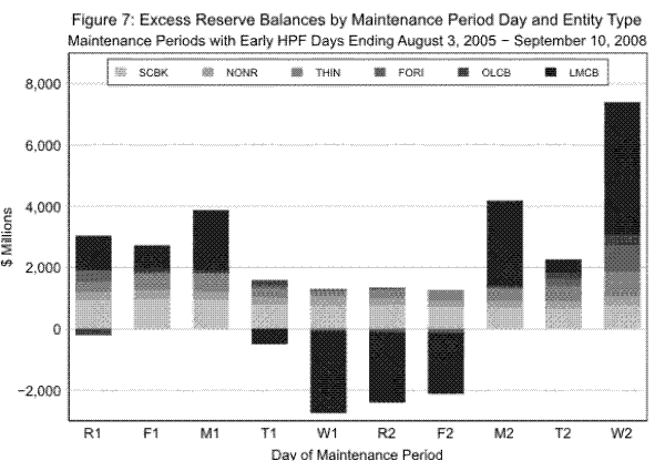
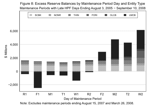
Second, we conjecture that, relative to cumulative excess observed at the time of the forecast, overall PAE will be higher if days with higher demand for excess are yet to come and lower if days with higher demand for excess are already in the past. Indeed, as shown in figures 7 and 8, the pattern of excess varies considerably depending on where the high payment flow days fall in the period. As can be seen in figures 7 and 8, the patterns are quite different, especially on the first Monday and both Fridays.
Third, we add two indicator variables to control for the differential patterns of reserve balance demand observed during periods when an FOMC meeting occurs and a rate increase is expected. As documented in Carpenter and Demiralp (2006a), in such periods, DIs have an incentive to hold higher balances earlier in the maintenance period, when rates are presumed to be lower.19 The earlier demand for reserve balances is known as the anticipation effect. The first indicator variable controls for the occurrence of an FOMC meeting at which a rate increase is expected at any point during the period; the second indicator variable controls for FOMC meetings that fall during the last three days of the period.
The final set of columns in table 3 detail our results. The point estimates indicate that the anticipation effect does not appear to influence demand for excess reserve balances for the period as a whole. In results not shown, we find that these coefficients are significant only at the ten percent level, but they do move in the expected directions.
Forecast performance
Because the models for period average excess demand presented in this paper are among a range of inputs that have traditionally contributed to monetary policy implementation decisions, it is critical that their usefulness as forecasting tools be determined. In order to evaluate our forecasting
tools, we re-calculate the coefficients in equations (1) and (2) using 40 maintenance periods (approximately 1
![]() years of data), and then forecast PAE for the remaining 13 maintenance periods (about six months)
during the pre-market turmoil sample. In addition, we compare forecast performance of the models in this paper to a rule of thumb that uses simply the sample mean PAE. We repeat this exercise with a sample that extends through the market turmoil period.
years of data), and then forecast PAE for the remaining 13 maintenance periods (about six months)
during the pre-market turmoil sample. In addition, we compare forecast performance of the models in this paper to a rule of thumb that uses simply the sample mean PAE. We repeat this exercise with a sample that extends through the market turmoil period.
Table 4 (a) presents the mean absolute errors (MAEs) and the root mean square errors (RMSEs) associated with each method for the pre-market turmoil sample. The left panel of the table shows the in-sample MAEs and RMSEs, while the right panel displays these statistics for the forecast sample. While the ex ante method performs reasonably well for the in-sample estimation, somewhat surprisingly, using simply the mean PAE performs better in a forecasting exercise. Inspection of the coefficients on the forecasting subsample, not shown, reveals a change in the coefficient on LMCB carryin, although one cannot reject the hypotheses that either coefficient is equal to one. This change in coefficient likely affects the forecast performance, and it is likely the case that in larger samples, these estimates would converge. In practice, we generally update the coefficients each period and forecast for only the current period; as a result, we feel that the ex ante regression model performs better than using simply average PAE over the past year and a half.
As shown under the Day 9 and Day 12 headings, incoming information clearly improves the ability to forecast PAE. In out-of-sample forecasting, the RMSE for the final specification falls about $100 million from the ex ante forecast to day 9, and another $30 million from day 9 to day 12. The final regression specification achieves an RMSE of about $140 million, about half that of the ex ante method. The $140 million difference in RMSE amounts to about $2 billion in excess on a single day basis, not a trivial sum. It should come as no surprise that as the end of the period approaches, it is easier to forecast period average excess. Still, a substantial portion of excess is held in the final three days of the period, and it is thus critical to be able to forecast demand over these days accurately.
Table 4(b) shows that incoming information clearly improves the ability to forecast PAE in the longer sample as well. In out-of-sample forecasting, the RMSE for the final specification falls about $180 million from the ex ante forecast to day 9, and another $110 million from day 9 to day 12. The final regression specification achieves an RMSE of about $230 million, substantially greater than the RMSE of the shorter sample but still less than about half that of the ex ante method. The $290 million difference in RMSE amounts to about $4 billion in excess on a single day basis. Although forecasting performance deteriorated using the longer sample, the regression approach still provided a substantial improvement over other rule-of-thumb methods.
Discussion and Conclusion
This paper provides new estimates of banks' demand for excess reserve balances on a period average basis. Consistent with theoretical work, we find that the demand for excess depends critically on uncertainty of flows in and out of reserve accounts, as evidenced by the significance of the number of high payment flow days within a reserve maintenance period. We also document facts concerning the demand for excess and how this differs according to the size of an institution, as well as evaluate different models for forecasting demand for excess on a period average basis and reporting the forecasting performance of each of these models.
References
Bartolini, Leonardo, Bertola, Giuseppe, and Prati, Alessandro. 2001. "Banks' Reserve Management, Transaction Costs, and the Timing of Federal Reserve Intervention," Journal of Banking and Finance, vol. 25 (July), p. 1287-1317.
Carpenter, Seth and Demiralp, Selva. 2006a. "Anticipation of Monetary Policy and Open Market Operations," International Journal of Central Banking, vol. 2, no. 2 (June), p. 25-63.
Carpenter, Seth and Demiralp, Selva. 2006b. "The Liquidity Effect in the Federal Funds Market: Evidence from Daily Open Market Operations," Journal of Money, Credit, and Banking, vol. 38 (June), p. 901-920.
Clouse, James and Dow, James P. Jr. 1999. "Fixed Costs and the Behavior of the Federal Funds Rate," Journal of Banking and Finance, vol. 23 (1999), p. 1015-1029.
Clouse, James, and Dow, James P. Jr. 2002. "A Computational Model of Banks' Optimal Reserve Management Policy," Journal of Economic Dynamics and Control, vol. 26 (September), p. 1787-1814.
Dow, James P. Jr. 2001. "The Demand for Excess Reserves," Southern Economic Journal, vol. 67, no. 3 (January), p. 685-700.
Evanoff, Douglas D. 1990. "An Empirical Examination of Bank Reserve Management Behavior," Journal of Banking and Finance, vol. 14, p. 131-143.
Federal Reserve System. 2006. Reserve Maintenance Manual. November.
Federal Reserve Bank of New York. 2007. Domestic Open Market Operations in 2006. February.
Hamilton, James D. 1997. "Measuring the Liquidity Effect," American Economic Review, vol. 87, p. 80-97.
Hamilton, James D. 1998. "The Supply and Demand for Federal Reserve Deposits," Carnegie-Rochester Conference Series on Public Policy, vol. 49, p. 1-44.
Judson, Ruth A., and Klee, Elizabeth. 2008. "Whither the Liquidity Effect? The impact of Federal Reserve Open Market operations in recent years," mimeo, April.
Poole, William. 1968. "Commercial Bank Reserve Management in a Stochastic Model: Implications for Monetary Policy," Journal of Finance, vol. 23, no. 5 (December), p. 769-791.
| Period Average Excess Reserve Balances Mean | Period Average Excess Reserve Balances Std. Dev. | Period Average Excess Reserve Balances Maximum | Period Average Excess Reserve Balances Minimum | Period Average Excess Reserve Balances Coeff. Of Variation | Period Average Excess Reserve Balances Share of Total Excess | |
|---|---|---|---|---|---|---|
| Entity Type: Total | 1727 | 366 | 3095 | 796 | 0.21 | 1 |
| Entity Type: LMCB | 79 | 247 | 1026 | -447 | 3.11 | 0.05 |
| Entity Type: OLCB | 61 | 62 | 302 | -65 | 1.02 | 0.04 |
| Entity Type: SCBK | 827 | 100 | 1101 | 631 | 0.12 | 0.48 |
| Entity Type: THIN | 424 | 132 | 855 | 138 | 0.31 | 0.25 |
| Entity Type: FORI | 91 | 59 | 269 | -22 | 0.65 | 0.05 |
| Entity Type: NONR | 246 | 66 | 525 | 179 | 0.27 | 0.14 |
| N | 79 | 79 | 79 | 79 | 79 | 79 |
| Required Operating Balances Mean | Required Operating Balances Std. Dev. | Required Operating Balances Maximum | Required Operating Balances Minimum | Required Operating Balances Coeff. Of Variation | Required Operating Balances Share of Total Excess | |
|---|---|---|---|---|---|---|
| Entity Type: Total | 14783 | 1854 | 20095 | 11904 | 0.13 | 1 |
| Entity Type: LMCB | 7060 | 1196 | 11807 | 5351 | 0.17 | 0.48 |
| Entity Type: OLCB | 1316 | 212 | 1845 | 802 | 0.16 | 0.09 |
| Entity Type: SCBK | 3139 | 652 | 4595 | 2149 | 0.21 | 0.21 |
| Entity Type: THIN | 2270 | 303 | 3053 | 1695 | 0.13 | 0.15 |
| Entity Type: FORI | 828 | 96 | 1175 | 694 | 0.12 | 0.06 |
| Entity Type: NONR | 171 | 94 | 340 | -478 | 0.55 | 0.01 |
| N | 79 | 79 | 79 | 79 | 79 | 79 |
| Ratio of Excess Reserve Balances to Required Operating Balances Mean | Ratio of Excess Reserve Balances to Required Operating Balances Std. Dev. | Ratio of Excess Reserve Balances to Required Operating Balances Maximum | Ratio of Excess Reserve Balances to Required Operating Balances Minimum | |
|---|---|---|---|---|
| Entity Type: Total | 0.12 | 0.03 | 0.2 | 0.06 |
| Entity Type: LMCB | 0.01 | 0.04 | 0.13 | -0.08 |
| Entity Type: OLCB | 0.05 | 0.04 | 0.21 | -0.05 |
| Entity Type: SCBK | 0.27 | 0.06 | 0.46 | 0.16 |
| Entity Type: THIN | 0.19 | 0.05 | 0.36 | 0.05 |
| Entity Type: FORI | 0.11 | 0.07 | 0.3 | -0.03 |
| Entity Type: NONR | 1.47 | 0.7 | 4.41 | -1 |
| N | 79 | 79 | 79 | 79 |
| Total Excess | LMCB Excess | OLCB Excess | THIN Excess | SCBK Excess | FORI Excess | NONR Excess | |
|---|---|---|---|---|---|---|---|
| LMCBCarry-in Coefficient | -0.6 | -0.81 | |||||
| LMCBCarry-in T-Statistic | -2.53* | -5.16* | |||||
| SumSpec1 Coefficient | 161.56 | 67.22 | 6.79 | 15.28 | 33.38 | 6.1 | 23.55 |
| SumSpec1 T-Statistic | 3.99* | 2.86* | 0.92 | 0.71 | 2.76* | 0.93 | 2.64* |
| Miss Coefficient | 0.08 | 0.05 | 0.01 | 0.02 | 0.01 | 0 | 0 |
| Miss T-Statistic | 3.16* | 3.30* | 0.82 | 2.13* | 0.64 | -0.03 | -1 |
| Constant Coefficient | 1480.6 | -15.34 | 50.8 | 404.43 | 772.66 | 80.94 | 204.99 |
| Constant T-Statistic | 19.36* | -0.4 | 3.74* | 9.70* | 32.72* | 6.94* | 14.89* |
| Observations | 79 | 79 | 79 | 79 | 79 | 79 | 79 |
| R2 | 0.35 | 0.41 | 0.03 | 0.07 | 0.1 | 0.01 | 0.09 |
*Significant at 5 percent level.
| Baseline Day 9 | Baseline Day 12 | Inter-mediate Day 9 | Inter-mediate Day 12 | Final Day 9 | Final Day 12 | |
|---|---|---|---|---|---|---|
| ExpectedOLCBPAE Coefficient | -0.14 | |||||
| ExpectedOLCBPAE T-Statistic | -0.23 | |||||
| ExpectedSCBKPAE Coefficient | 0.92 | 1.42 | 0.97 | 1.4 | 1 | 1.41 |
| ExpectedSCBKPAE T-Statistic | 4.26* | 7.49* | 4.40* | 7.88* | 4.90* | 7.70* |
| ExpectedTHINPAE (DRP) Coefficient | -0.91 | -0.71 | ||||
| ExpectedTHINPAE (DRP) T-Statistic | -1.41 | -1.46 | ||||
| ExpectedTHINPAE (Small) Coefficient | 1.1 | 1.07 | ||||
| ExpectedTHINPAE (Small) T-Statistic | 6.00* | 8.69* | ||||
| ExpectedTHINPAE Coefficient | 1.1 | 1.08 | 1.15 | 1.09 | ||
| ExpectedTHINPAE T-Statistic | 5.92* | 9.19* | 6.78* | 8.66* | ||
| ExpectedNONRPAE Coefficient | 0.37 | 0.9 | 0.28 | 0.74 | 0.48 | 0.75 |
| ExpectedNONRPAE T-Statistic | 1.95 | 5.00* | 1.44 | 3.46* | 2.15* | 3.03* |
| ExpectedFORIPAE (DRP) Coefficient | 3.2 | 4.64 | ||||
| ExpectedFORIPAE (DRP) T-Statistic | 0.75 | 4.70* | ||||
| ExpectedFORIPAE (Small) Coefficient | 0.27 | 0.58 | ||||
| ExpectedFORIPAE (Small) T-Statistic | 0.69 | 1.57 | ||||
| AdjustedLMCBLockins Coefficient | 1.16 | 0.87 | 1.17 | 1.17 | 1.12 | 1.15 |
| AdjustedLMCBLockins T-Statistic | 2.65* | 6.23* | 3.29* | 5.32* | 3.38* | 5.71* |
| LMCBCarry-in Coefficient | -1.16 | -0.93 | -1.25 | -1.06 | -1.19 | -1.04 |
| LMCBCarry-in T-Statistic | -5.68* | -7.15* | -7.33* | -8.67* | -7.25* | -8.26* |
| LateHPF Coefficient | 194.49 | 108.29 | ||||
| LateHPF T-Statistic | 3.72* | 2.82* | ||||
| FOMCAnticipation Coefficient | 89.26 | -25.71 | ||||
| FOMCAnticipation T-Statistic | 0.89 | -0.37 | ||||
| FOMCAnticipationwith late-periodFOMCmeeting Coefficient | -135.47 | 60.56 | ||||
| FOMCAnticipationwith late-periodFOMCmeeting T-Statistic | -1.18 | 0.65 | ||||
| Constant Coefficient | 393.83 | -178.05 | 367.59 | -138.5 | 190.26 | -189.59 |
| Constant T-Statistic | 2.24* | -1.15 | 2.16* | -0.89 | 1.14 | -1.22 |
| R2 | 0.64 | 0.85 | 0.62 | 0.8 | 0.68 | 0.82 |
| N | 79 | 79 | 79 | 79 | 79 | 79 |
*Significant at 5 percent level.
| In-sample statistics (Fitted values over full sample) MAE | In-sample statistics (Fitted values over full sample) RMSE | Out-of sample statistics (Fitted values over forecast sample) MAE | Out-of sample statistics (Fitted values over forecast sample) RMSE | |
| Mean | 274.409 | 323.819 | 189.214 | 239.393 |
| Ex ante | 163.214 | 211.363 | 230.513 | 271.684 |
| Day 9: First regression | 124.621 | 163.909 | 183.444 | 212.67 |
| Day 9: Final regression | 122.845 | 168.094 | 140.196 | 169.814 |
| Day 12: First regression | 75.218 | 100.928 | 120.716 | 163.12 |
| Day 12: Final regression | 78.895 | 98.714 | 107.47 | 138.906 |
| N | 40 | 40 | 40 (fitted sample), 13 (forcast sample) | 40 (fitted sample), 13 (forcast sample) |
| In-sample statistics (Fitted values over full sample) MAE | In-sample statistics (Fitted values over full sample) RMSE | Out-of sample statistics (Fitted values over forecast sample) MAE | Out-of sample statistics (Fitted values over forecast sample) RMSE | |
|---|---|---|---|---|
| Mean | 261.526 | 329.965 | 398.319 | 524.545 |
| Ex ante | 184.395 | 233.786 | 399.587 | 521.178 |
| Day 9: First regression | 152.296 | 195.843 | 238.026 | 339.414 |
| Day 9: Final regression | 136.014 | 180.702 | 258.701 | 340.835 |
| Day 12: First regression | 112.084 | 139.058 | 161.458 | 217.213 |
| Day 12: Final regression | 113.148 | 143.213 | 201.51 | 228.958 |
| N | 66 | 66 | 66 (fitted sample), 13 (forecast sample) | 66 (fitted sample), 13 (forecast sample) |
