
What is the Chance that the Equity Premium Varies over Time?
Evidence from Predictive Regressions *
Keywords: Equity premium, return predictability, Bayesian methods
Abstract:
1 Introduction
This paper investigates the evidence in favor of stock return predictability from a model-selection perspective. Much recent empirical work has focused on the predictive regression
where
One approach to investigating whether stock returns are predictable involves running an ordinary least squares regression (OLS) on (1) and asking whether the predictive coefficient ![]() is significantly different from zero. As emphasized in a simulation study by Kandel and Stambaugh (1996), however, this approach has the disadvantage that classical significance may not be indicative of whether the level of
predictability is of economic significance. If
is significantly different from zero. As emphasized in a simulation study by Kandel and Stambaugh (1996), however, this approach has the disadvantage that classical significance may not be indicative of whether the level of
predictability is of economic significance. If ![]() is found to be insignificant, or only marginally significant, one cannot conclude that predictability "does not exist" as far as
economic agents are concerned.
is found to be insignificant, or only marginally significant, one cannot conclude that predictability "does not exist" as far as
economic agents are concerned.
In this study we adopt a Bayesian approach to inference on (1) that takes model uncertainty as well as parameter uncertainty into account. An investor evaluates the evidence in favor of equation (1) as opposed to a null hypothesis
The investor assigns a prior probability
Our paper builds on several strands of the recent portfolio allocation literature. Once such strand studies properties of Bayesian estimation of predictive regressions (e.g. Barberis (2000), Johannes, Polson, and Stroud (2002), Brandt, Goyal, Santa-Clara, and Stroud (2005), Pastor and Stambaugh (2008), Skoulakis (2007), Stambaugh (1999), Wachter and Warusawitharana (2009)), but assumes that the predictive model is known. A second strand focuses on model uncertainty, but assumes that the parameters within the model are known (e.g. Chen, Ju, and Miao (2009), Maenhout (2006), Hansen (2007)). A third strand allows for both model and parameter uncertainty, but assumes returns are independent and identically distributed (e.g. Chen and Epstein (2002), Garlappi, Uppal, and Wang (2007)).1 Our paper builds on this work by assuming that the investor faces both parameter and model uncertainty, and considers the possibility that returns are predictable.
Our paper also builds on the literature on return predictability and model selection (Pesaran and Timmermann (1995), Avramov (2002), Cremers (2002)); these papers make the assumption that the future time path of the regressor is known, an assumption that is frequently satisfied in a standard ordinary least squares regression, but rarely satisfied in a predictive regression. By making use of methods developed in Wachter and Warusawitharana (2009), we are able to formulate and solve the investor's problem when the regressor is stochastic. Our paper therefore incorporates the insights of the frequentist literature on predictive return regressions (e.g. Cavanagh, Elliott, and Stock (1995), Nelson and Kim (1993), Stambaugh (1999), Lewellen (2004), Torous, Valkanov, and Yan (2004), Campbell and Yogo (2006)) into a Bayesian portfolio selection setting.
When we apply our methods to predicting returns by the dividend-price ratio, we find that an investor who believes that there is a 20% probability of predictability prior to seeing the data updates to a 65% posterior probability after viewing quarterly postwar data. An advantage of modeling the stochastic process for the regressor is that we are able to compute certainty equivalent returns from exploiting predictability that do not depend on a particular value for the regessor. We find certainty equivalent returns of 1.16% per year when the dividend-price ratio is used as a predictor variable for an investor whose prior probability in favor of predictability is just 20%. For an investor who believes that there is a 50/50 chance of return predictability, certainty equivalent returns are 1.83%.
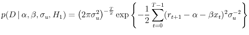
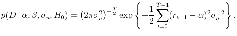
We also empirically evaluate the effect of using a full Bayes, exact likelihood approach as opposed to the conditional likelihood, and as opposed to empirical Bayes. A common approach to Bayesian inference in a time series setting is to treat the first observation of the predictor variable as a known parameter rather than a draw from the data generating process. However, we find that conditioning on the first observation results in Bayes factors (the ratio of the likelihood of model (1) to (2)) that are substantially smaller as compared to when the initial observation is treated as a draw from the data generating process. The posterior for the unconditional risk premium is highly unstable when we condition on the first observation. However, when this is treated as a draw from the data generating process, the expected return is estimated in a reliable way. In addition, using an empirical Bayes approach, which involves using data on the regressor to determine the prior, implies Bayes factors that are larger than those implied by the fully Bayesian approach. Conditioning on the first observation and using empirical Bayes are often regarded as approximation techniques to the full Bayes exact likelihood approach that we emphasize (e.g. Box and Tiao (1973), Chipman, George, and McCulloch (2001)). Our results suggest that, at least for some purposes, this approximation may be less accurate than previously believed.
2.1 Data generating processes
Let ![]() denote continuously compounded excess returns on a stock index from time
denote continuously compounded excess returns on a stock index from time ![]() to
to ![]() and
and ![]() the value of a (scalar) predictor variable. We
assume that this predictor variable follows the process
the value of a (scalar) predictor variable. We
assume that this predictor variable follows the process
Stock returns can be predictable, in which case they follow the process (1) or unpredictable, in which case they follow the process (2). In either case, errors are serially uncorrelated, homoskedastic, and jointly normal:
![\displaystyle \left[\begin{array}{c} u_{t+1} v_{t+1} \end{array}\right] \vert r_t,\ldots, r_1, x_t, \ldots, x_0 \sim N\left( 0,\Sigma \right),](img18.gif)
and
![\displaystyle \Sigma = \left[\begin{array}{cc} \sigma_u^2 & \sigma_{uv} \sigma_{uv} & \sigma_v^2 \end{array}\right].](img19.gif)
As we show below, the correlation between innovations to returns and innovations to the state variable implies that (3) affects inference about returns, even when there is no predictability.
When the process (3) is stationary, i.e. ![]() is between -1 and 1, the state variable has an unconditional mean of
is between -1 and 1, the state variable has an unconditional mean of

and a variance of
These follow from taking unconditional means and variances on either side of (3). Note that these are population values conditional on knowing the parameters. Given these, the population
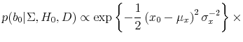
2.2 Prior Beliefs
An investor's prior views on predictability can be elicited by the answer to two straightforward questions.2 Consider data generating processes of the form (1) and (2). Given these processes, the investor should answer:
- [Question 1] What is the probability that predictability exists, i.e. that equation (1) describes returns for some
 ? (Call this answer
  .)
.) - [Question 2] Given that predictability exists, what is the probability that the
 exceeds 1%? (Call this answer
  .)
.)
We now demonstrate how to specify priors given the answers to these questions. An appeal of this approach is that it is not necessary to specify aspects of the distribution of the predictor variable and of returns other than those given above. The prior beliefs are invariant to changes to these aspects of the distribution.
2.2.1 Full Bayes priors
Let ![]() denote the state of the world in which excess returns are unpredictable (the "null") and
denote the state of the world in which excess returns are unpredictable (the "null") and ![]() denote the state of the world in which there is some amount of excess return predictability. Then
denote the state of the world in which there is some amount of excess return predictability. Then ![]() is the prior probability of
is the prior probability of ![]() , i.e.
, i.e.
![]() . In what follows, we construct priors for the parameters conditional on
. In what follows, we construct priors for the parameters conditional on ![]() and on
and on ![]() . It is convenient to group the regression parameters in equations (1), (2) and (3) into vectors
. It is convenient to group the regression parameters in equations (1), (2) and (3) into vectors
Note that
![]() can also be written as
can also be written as
![]() . We set the prior on
. We set the prior on ![]() and
and ![]() so that
so that
for
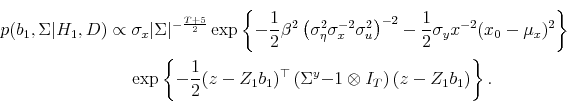
The parameter that distinguishes ![]() from
from ![]() is
is ![]() . One approach would be to write down a prior distribution for
. One approach would be to write down a prior distribution for ![]() unconditional on the remaining
parameters. However, it is difficult to think about priors on
unconditional on the remaining
parameters. However, it is difficult to think about priors on ![]() in isolation from beliefs about other parameters. For example, a high variance of
in isolation from beliefs about other parameters. For example, a high variance of ![]() might lower one's prior on
might lower one's prior on ![]() , while a large residual variance of
, while a large residual variance of ![]() might raise it. Rather than placing a prior on
might raise it. Rather than placing a prior on ![]() directly, we follow Wachter and Warusawitharana
(2009) and place a prior on the population
directly, we follow Wachter and Warusawitharana
(2009) and place a prior on the population ![]() . To implement this prior on the
. To implement this prior on the ![]() , we place a prior on "normalized"
, we place a prior on "normalized" ![]() , that is
, that is ![]() adjusted for the variance of
adjusted for the variance of ![]() and the variance of
and the variance of ![]() . Let
. Let
The population
Equation (10) provides a mapping between a prior distribution on
A prior on ![]() implies a hierarchical prior on
implies a hierarchical prior on ![]() . Because
. Because
where
Jeffreys invariance theory provides an independent justification for modeling priors on ![]() as (11). Stambaugh (1999) shows that the
limiting Jeffreys prior for
as (11). Stambaugh (1999) shows that the
limiting Jeffreys prior for ![]() and
and ![]() equals
equals
This prior corresponds to the limit of (12) as
Figure C shows the resulting distribution for the population ![]() for various values of
for various values of
![]() . Panel A shows the distribution conditional on
. Panel A shows the distribution conditional on ![]() while
Panel B shows the unconditional distribution. More precisely, for any value
while
Panel B shows the unconditional distribution. More precisely, for any value ![]() , Panel A shows the prior probability that the
, Panel A shows the prior probability that the ![]() exceeds
exceeds ![]() , conditional on the existence of predictability. For large values of
, conditional on the existence of predictability. For large values of
![]() , e.g. 100, the prior probability that the
, e.g. 100, the prior probability that the ![]() exceeds
exceeds ![]() across the relevant range of values for the
across the relevant range of values for the ![]() is close to one. The lower the value of
is close to one. The lower the value of
![]() , the less variability in
, the less variability in ![]() around its mean of zero, and the lower
the probability that the
around its mean of zero, and the lower
the probability that the ![]() exceeds
exceeds ![]() for any value of
for any value of ![]() . Panel B shows the unconditional probability that the
. Panel B shows the unconditional probability that the ![]() exceeds
exceeds ![]() for any value of
for any value of ![]() , assuming that the prior probability of predictability,
, assuming that the prior probability of predictability, ![]() , is equal to 0.5. By the definition of conditional probability:
, is equal to 0.5. By the definition of conditional probability:
2.2.2 Empirical Bayes priors
A second approach to formulating priors involves conditioning on moments of the data. Let ![]() denote the length of the sample and
denote the length of the sample and
![]() the sample variance of
the sample variance of ![]() :
:
where
The specification is completed by setting
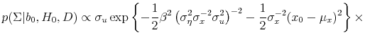
These assumptions on the prior are combined with the likelihood
and
Very similar specifications are employed by Chipman, George, and McCulloch (2001), Cremers (2002), Wright (2003) and Stock and Watson (2005). Note that these equations display the marginal likelihood over the return equations (1) and (2) rather than the full likelihood that includes the data generating process for
The above assumptions are most reasonable in the case where
![]() are observed at time 0. While this holds in many applications of OLS regression, it holds rarely, if ever, in the case of predictive regressions in financial time series.
Moreover, were
are observed at time 0. While this holds in many applications of OLS regression, it holds rarely, if ever, in the case of predictive regressions in financial time series.
Moreover, were
![]() observed, the contemporaneous correlation between
observed, the contemporaneous correlation between ![]() and
and
![]() would invalidate the likelihoods (17) and (18) because the value of
would invalidate the likelihoods (17) and (18) because the value of ![]() would convey information about
would convey information about ![]() not reflected in these likelihoods. One way to interpret the above in the setting where
not reflected in these likelihoods. One way to interpret the above in the setting where ![]() is stochastic is to assume that, while the data on
is stochastic is to assume that, while the data on ![]() themselves are unobserved, certain
functions of the data, namely sample moments of
themselves are unobserved, certain
functions of the data, namely sample moments of ![]() such as
such as
![]() , are observed. Allowing data to influence the prior is generally referred to as the "empirical Bayes" method.4 For this reason, the formulation of priors that use moments from the sample could be thought of as an example of empirical Bayes, at least if one accepts a broad definition of the term.5
, are observed. Allowing data to influence the prior is generally referred to as the "empirical Bayes" method.4 For this reason, the formulation of priors that use moments from the sample could be thought of as an example of empirical Bayes, at least if one accepts a broad definition of the term.5
Regardless of its theoretical attractiveness, it is of interest to ask whether the use of empirical Bayes in this setting make a difference in practice. There are a number of differences between the specification described in (14)-(18) and
ours. Most importantly, by assuming the investor knows the sample moments of ![]() , the above approach avoids the need to make explicit assumptions on the prior for the parameters of the
, the above approach avoids the need to make explicit assumptions on the prior for the parameters of the
![]() process and for the likelihood of the
process and for the likelihood of the ![]() process. However, as we show, these
assumptions, whether hidden or explicit, have important consequences for the posterior distribution.
process. However, as we show, these
assumptions, whether hidden or explicit, have important consequences for the posterior distribution.
Leaving these issues aside for the moment, our immediate goal is to write down a version of the above specification that is close enough to our model so that differences in results stemming from the link (or lack thereof) between the distribution of ![]() and that of
and that of ![]() can be interpreted. To this end, we consider the specification
can be interpreted. To this end, we consider the specification
We assume a standard uninformative prior for the remaining parameters (see Zellner (1996) and Gelman, Carlin, Stern, and Rubin (2004)): with a normal distribution for ![]() , where the prior covariance reflects the agent's beliefs about predictability. We also ensure that
, where the prior covariance reflects the agent's beliefs about predictability. We also ensure that ![]() is stationary. That is:
is stationary. That is:
for
These priors may be thought of as the simplest set of priors which contain information about the distribution of
2.3.1 Likelihood under 
Under ![]() , returns and the state variable follow the joint process given in (1) and (3). It is convenient to group observations on
returns and contemporaneous observations on the state variable into a matrix
, returns and the state variable follow the joint process given in (1) and (3). It is convenient to group observations on
returns and contemporaneous observations on the state variable into a matrix ![]() and lagged observations on the state variable and the constant into a matrix
and lagged observations on the state variable and the constant into a matrix ![]() . Let
. Let
![\displaystyle Y = \left[\begin{array}{cc}r_1 & x_1 \vdots & \vdots \ r_T & x_T \end{array} \right] X = \left[\begin{array}{cc}1 & x_0 \vdots & \vdots 1 & x_{T-1} \end{array} \right],](img85.gif)
In the above, the
(see Zellner (1996)).
The likelihood function (21) conditions on the first observation of the predictor variable, ![]() . Stambaugh (1999) argues for treating
. Stambaugh (1999) argues for treating
![]() and
and
![]() symmetrically: as random draws from the data generating process. If the process for
symmetrically: as random draws from the data generating process. If the process for ![]() is stationary and has run for a substantial period of time, then results in (Hamilton, 1994, p. 265) imply that
is stationary and has run for a substantial period of time, then results in (Hamilton, 1994, p. 265) imply that ![]() is a draw from a
multivariate normal distribution with mean
is a draw from a
multivariate normal distribution with mean ![]() and standard deviation
and standard deviation ![]() .
Combining the likelihood of the first observation with the likelihood of the remaining
.
Combining the likelihood of the first observation with the likelihood of the remaining ![]() observations produces
observations produces
Following Box and Tiao (1973), we refer to (21) as the conditional likelihood and (22) as the exact likelihood.
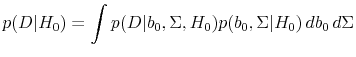
2.3.2 Likelihood under 
Under ![]() , returns and the state variable follow the processes given in (2) and (3). Let
, returns and the state variable follow the processes given in (2) and (3). Let
![\displaystyle Z_0 = \left[\begin{array}{cc} \iota_T & 0_{T\times 2} 0_{T\times 1} & X \end{array}\right],](img95.gif)
Using similar reasoning as in the
As above, we refer to (23) as the conditional likelihood and (24) as the exact likelihood.
2.4 Posterior distribution
The investor updates his prior beliefs to form the posterior distribution upon seeing the data. As we discuss below, this posterior requires the computation of two quantities: the posterior of the parameters conditional on the absence or existence of return predictability, and the posterior probability that returns are predictable. Given these two quantities, we can simulate from the posterior distribution.
To compute the posteriors conditional on the absence or existence of return predictability, we apply Bayes' rule conditioning on ![]() and conditioning on
and conditioning on ![]() . It follows from Bayes' rule that
. It follows from Bayes' rule that
is the posterior conditional on
is the posterior conditional on
Let ![]() denote the posterior probability that excess returns are predictable. By definition,
denote the posterior probability that excess returns are predictable. By definition,
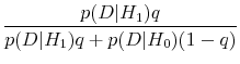
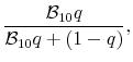
where
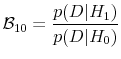
is the Bayes factor for the alternative hypothesis of predictability against the null of no predictability. The Bayes factor is a likelihood ratio in that it is the likelihood of return predictability divided by the likelihood of no predictability. However, it differs from the standard likelihood ratio in that the likelihoods
and
To form
Putting these two pieces together, we draw from the posterior parameter distribution by drawing from
![]() with probability
with probability ![]() and from
and from
![]() with probability
with probability ![]() .
.
3 Results
We now apply the above framework to understanding the predictive power of the dividend-price ratio and payout yield for the excess return on a broad equity index.
3.1 Data
We use data from the Center for Research on Security Prices (CRSP). We compute excess stock returns by subtracting the continuously compounded 3-month treasury bill return from the return on the value-weighted CRSP index at annual and quarterly frequencies. Following a large portfolio selection literature (see, e.g., Brennan, Schwartz, and Lagnado (1997), Campbell and Viceira (1999)), we focus on the dividend-price ratio as the predictive factor. The dividend-price ratio is computed by dividing the dividend payout over the previous 12 months with the current price of the stock index. The use of 12 months of data accounts for seasonalities in dividend payments. We use the logarithm of the dividend-price ratio as the predictive factor. We also use the repurchases-adjusted payout yield of Boudoukh, Michaely, Richardson, and Roberts (2007) as a predictive factor. Data are annual data from 1927 to the beginning of 2005; we also report results with the dividend-price ratio at a quarterly frequency from 1952 onwards.
3.2 Bayes factors and posterior means
Table 1 reports Bayes factors and posterior means when the payout yield is used as a predictor variable. Table 2 and 3 report analogous results for the dividend-price ratio in annual data and in quarterly
postwar data respectively. Each table reports results for full Bayes priors combined with the exact likelihood, for full Bayes priors combined with the conditional likelihood and for empirical Bayes priors combined with the exact likelihood. For each prior and likelihood combination, four values of
![]() are considered: 0.05, 0.09, 0.15 and 100. For the full Bayes priors, these translate into values of
are considered: 0.05, 0.09, 0.15 and 100. For the full Bayes priors, these translate into values of ![]() (the prior probability that the
(the prior probability that the ![]() exceeds 0.01) equal to 0.05, 0.25, 0.50 and 0.99 respectively. For the empirical Bayes priors, the prior distribution
over the
exceeds 0.01) equal to 0.05, 0.25, 0.50 and 0.99 respectively. For the empirical Bayes priors, the prior distribution
over the ![]() is not well defined. We construct these priors using the same values of
is not well defined. We construct these priors using the same values of
![]() as the full Bayes counterparts. Because the results are qualitatively similar across the three data sets, we focus on results for the payout yield in Table 1.
as the full Bayes counterparts. Because the results are qualitatively similar across the three data sets, we focus on results for the payout yield in Table 1.
Table 1 shows that the Bayes factor is hump-shaped in ![]() for each prior-likelihood combination. For small values of
for each prior-likelihood combination. For small values of ![]() , the Bayes factor is close to one. For large values, the Bayes factor is close to zero. Both results can be understood using the formula for the Bayes factor in (28) and for the likelihoods
, the Bayes factor is close to one. For large values, the Bayes factor is close to zero. Both results can be understood using the formula for the Bayes factor in (28) and for the likelihoods
![]() and
and
![]() in (29) and (30). For low values of
in (29) and (30). For low values of ![]() , the investor imposes a very tight prior on the
, the investor imposes a very tight prior on the ![]() . Therefore the hypotheses that returns are predictable and that returns are unpredictable are nearly the same. It
follows from (29) and (30) that the likelihoods of the data under these two scenarios are nearly the same and that the Bayes factor is nearly one. This is intuitive: when two hypotheses are close, a great deal of data are required to distinguish one
from the other.
. Therefore the hypotheses that returns are predictable and that returns are unpredictable are nearly the same. It
follows from (29) and (30) that the likelihoods of the data under these two scenarios are nearly the same and that the Bayes factor is nearly one. This is intuitive: when two hypotheses are close, a great deal of data are required to distinguish one
from the other.
The fact that the Bayes factor approaches zero as ![]() increases is less intuitive. The reduction in Bayes factors implies that, as the investor allows a greater range of values for the
increases is less intuitive. The reduction in Bayes factors implies that, as the investor allows a greater range of values for the
![]() , the posterior probability that returns are predictable approaches zero. This effect is known as Bartlett's paradox, and was first noted by Bartlett (1957) in the
context of distinguishing between uniform distributions. As Kass and Raftery (1995) discuss, Bartlett's paradox makes it crucial to formulate an informative prior on the parameters that differ between
, the posterior probability that returns are predictable approaches zero. This effect is known as Bartlett's paradox, and was first noted by Bartlett (1957) in the
context of distinguishing between uniform distributions. As Kass and Raftery (1995) discuss, Bartlett's paradox makes it crucial to formulate an informative prior on the parameters that differ between ![]() and
and ![]() . The mathematics leading to Bartlett's paradox are most easily seen in a case where Bayes factors can be computed in closed form. However, we
can obtain an understanding of the paradox based on the form of the likelihoods
. The mathematics leading to Bartlett's paradox are most easily seen in a case where Bayes factors can be computed in closed form. However, we
can obtain an understanding of the paradox based on the form of the likelihoods
![]() and
and
![]() . These likelihoods involve integrating out the parameters using the prior distribution. If the prior distribution on
. These likelihoods involve integrating out the parameters using the prior distribution. If the prior distribution on ![]() is highly uninformative, the prior places a large amount of mass in extreme regions of the parameter space. In these regions, the likelihood of the data conditional on the parameters will be quite small. At the same time, the prior places
a relatively small amount of mass in the regions of the parameter space where the likelihood of the data is large. Therefore
is highly uninformative, the prior places a large amount of mass in extreme regions of the parameter space. In these regions, the likelihood of the data conditional on the parameters will be quite small. At the same time, the prior places
a relatively small amount of mass in the regions of the parameter space where the likelihood of the data is large. Therefore
![]() (the integral of the likelihood under
(the integral of the likelihood under ![]() ) is small relative to
) is small relative to
![]() (the integral of the likelihood under
(the integral of the likelihood under ![]() ).
).
Table 1 also shows that there are substantial differences between the Bayes factors resulting from the exact versus the conditional likelihood and from empirical versus full Bayes. The Bayes factors resulting from the exact likelihood are larger than those resulting from the conditional likelihood, thus implying a greater posterior probability of return predictability. The Bayes factors resulting from full Bayes are smaller than those resulting from empirical Bayes, implying a lower posterior probability of return predictability.
In what follows, we seek to explain these patterns in the Bayes factors. Let
![]() be the posterior mean of
be the posterior mean of ![]() conditional on predictability and
conditional on predictability and
![]() the posterior mean of
the posterior mean of ![]() conditional on predictability. As
Table 1 shows, differences in Bayes factors between specifications reflect differences in
conditional on predictability. As
Table 1 shows, differences in Bayes factors between specifications reflect differences in
![]() . That is, for any given value of
. That is, for any given value of ![]() ,
,
![]() is higher for the exact likelihood than for the conditional likelihood, and lower for full Bayes than for empirical Bayes. Moreover, the opposite pattern is evident for
is higher for the exact likelihood than for the conditional likelihood, and lower for full Bayes than for empirical Bayes. Moreover, the opposite pattern is evident for
![]() . The negative correlation between
. The negative correlation between ![]() and
and ![]() is also noted by Stambaugh (1999)). The source of this negative relation is the negative correlation between shocks to returns and shocks to the predictor variable. Suppose
that a draw of
is also noted by Stambaugh (1999)). The source of this negative relation is the negative correlation between shocks to returns and shocks to the predictor variable. Suppose
that a draw of ![]() is below its value predicted by ordinary least squares (OLS). This implies that the OLS value for
is below its value predicted by ordinary least squares (OLS). This implies that the OLS value for ![]() is "too high", i.e. in the sample shocks to the predictor variable are followed by shocks to returns of the same sign. Therefore shocks to the predictor variable tend to be followed by shocks to the predictor variable that are of different signs. Thus the
OLS value for
is "too high", i.e. in the sample shocks to the predictor variable are followed by shocks to returns of the same sign. Therefore shocks to the predictor variable tend to be followed by shocks to the predictor variable that are of different signs. Thus the
OLS value for ![]() is "too low". This explains why values of
is "too low". This explains why values of
![]() are higher for low values of
are higher for low values of ![]() (and hence low values of
(and hence low values of
![]() ) than for high values, and higher than the ordinary least squares estimate.
) than for high values, and higher than the ordinary least squares estimate.
We can use the connection between
![]() ,
,
![]() and the Bayes factor to account for differences between the Bayes factors between the prior and likelihood specifications. As Table 1 shows, using
the exact likelihood leads to lower posterior values of
and the Bayes factor to account for differences between the Bayes factors between the prior and likelihood specifications. As Table 1 shows, using
the exact likelihood leads to lower posterior values of ![]() . This is because the exact likelihood leads to more precise estimates of
. This is because the exact likelihood leads to more precise estimates of ![]() . By the argument in the previous paragraph, this implies greater posterior values for
. By the argument in the previous paragraph, this implies greater posterior values for ![]() and higher Bayes factors.
and higher Bayes factors.
On the other hand, the use of full rather than empirical Bayes implies higher posterior values of ![]() . This occurs because the full Bayes prior, on account of the
. This occurs because the full Bayes prior, on account of the
![]() term, puts more weight on high values of
term, puts more weight on high values of ![]() and therefore high
values of
and therefore high
values of ![]() . When
. When ![]() is not far from zero, the posterior distribution is
higher for lower values of
is not far from zero, the posterior distribution is
higher for lower values of
![]() , and hence higher values of
, and hence higher values of ![]() . This leads to lower posterior
means of
. This leads to lower posterior
means of ![]() and lower Bayes factors.
and lower Bayes factors.
Tables 1-3 also report the posterior means of excess returns (the equity premium) and of the predictor variable conditional on predictability. In each case, the OLS row reports the sample mean of excess returns and the sample mean of the
predictor variable.7 Posterior means conditional on no predictability are very close to their counterparts for
![]() . Surprisingly, the various choices for the predictor variable and for the prior and likelihood imply different values for the equity premium. For example, the sample average
for excess returns over the 1927 to 2004 period is 5.85% per annum. In contrast, the full Bayes exact likelihood approach generates average returns that range from 5.05% to 5.24% per annum depending on the informativeness of the prior (the more informative the prior, the higher the excess
return).
. Surprisingly, the various choices for the predictor variable and for the prior and likelihood imply different values for the equity premium. For example, the sample average
for excess returns over the 1927 to 2004 period is 5.85% per annum. In contrast, the full Bayes exact likelihood approach generates average returns that range from 5.05% to 5.24% per annum depending on the informativeness of the prior (the more informative the prior, the higher the excess
return).
The differences in the estimates of the equity premium arise from differences in estimates of the mean of the predictor variable. The conditional maximum likelihood estimate of the mean of ![]() (not reported) is -3.54. The posterior mean implied by the exact likelihood is between -3.16 and -3.17 (depending on the prior). Thus according to the model, shocks to the predictor variable over the sample period must be negative for -3.54 to be the estimated value when the
conditional likelihood is used. It follows that the shocks to excess returns must be positive (because of the negative correlation). Therefore the posterior mean is below the sample mean. This effect also operates in the case of the dividend-price ratio and is in fact more dramatic. In annual data
from 1927 to 2004, the implied means for excess returns range from 4.02 to 4.71% per annum versus the sample mean of 5.85%.
(not reported) is -3.54. The posterior mean implied by the exact likelihood is between -3.16 and -3.17 (depending on the prior). Thus according to the model, shocks to the predictor variable over the sample period must be negative for -3.54 to be the estimated value when the
conditional likelihood is used. It follows that the shocks to excess returns must be positive (because of the negative correlation). Therefore the posterior mean is below the sample mean. This effect also operates in the case of the dividend-price ratio and is in fact more dramatic. In annual data
from 1927 to 2004, the implied means for excess returns range from 4.02 to 4.71% per annum versus the sample mean of 5.85%.
While the use of empirical Bayes implies values for the posterior mean of ![]() that are similar to those for full Bayes, the use of the conditional likelihood implies estimates that are
highly variable and can even be negative. This is because of the lack of precision in estimating
that are similar to those for full Bayes, the use of the conditional likelihood implies estimates that are
highly variable and can even be negative. This is because of the lack of precision in estimating ![]() .
.
Tables 1-3 demonstrate differences in the posterior distribution depending on whether one uses full Bayes or empirical Bayes, and whether one uses the exact likelihood or the conditional likelihood. In what follows, we will examine the full
Bayes, exact likelihood case more closely, and show its implications for inference on return predictability. The following two sections examine statistical measures: the posterior likelihood of predictability and the posterior distribution of the ![]() . The final section examines economic significance of the predictability evidence through certainty equivalent returns.
. The final section examines economic significance of the predictability evidence through certainty equivalent returns.
3.3 Posterior likelihood of predictability
We now examine the posterior probability that excess returns are predictable. Given a Bayes factor and a prior belief on the existence of predictability ![]() , the posterior probability of
predictability
, the posterior probability of
predictability ![]() can be computed using equation (27). The greater the investor's prior belief about predictability, the greater is his posterior belief. The
greater is the Bayes factor, the greater is the posterior belief. As described in the previous section, the Bayes factor itself depends on the other aspect of the investor's prior: the prior probability that the
can be computed using equation (27). The greater the investor's prior belief about predictability, the greater is his posterior belief. The
greater is the Bayes factor, the greater is the posterior belief. As described in the previous section, the Bayes factor itself depends on the other aspect of the investor's prior: the prior probability that the ![]() exceeds 1% should predictability exist.
exceeds 1% should predictability exist.
Table 4 presents the posterior probabilities of predictability as a function of the investor's prior about the existence of predictability, ![]() , and the prior
belief on the strength of predictability,
, and the prior
belief on the strength of predictability, ![]() . We consider the posterior resulting from full Bayes priors and the exact likelihood. The posterior probability is increasing in
. We consider the posterior resulting from full Bayes priors and the exact likelihood. The posterior probability is increasing in ![]() and hump-shaped in
and hump-shaped in ![]() , reflecting the fact that the Bayes factors are hump-shaped in
, reflecting the fact that the Bayes factors are hump-shaped in
![]() . The results demonstrate that investors with moderate beliefs on both the existence and strength of predictability revise their beliefs on the existence on predictability sharply
upward. For example, an investor with
. The results demonstrate that investors with moderate beliefs on both the existence and strength of predictability revise their beliefs on the existence on predictability sharply
upward. For example, an investor with ![]() and
and
![]() conclude that the posterior likelihood of predictability equals 0.88 using the payout yield to predict annual returns. This result is robust to a wide range of choices for
conclude that the posterior likelihood of predictability equals 0.88 using the payout yield to predict annual returns. This result is robust to a wide range of choices for
![]() . As the table shows,
. As the table shows,
![]() implies a posterior probability of 0.74. The posterior probability falls off dramatically as
implies a posterior probability of 0.74. The posterior probability falls off dramatically as ![]() approaches one; for these very diffuse priors (which imply what might be considered an economically unreasonable amount of predictability), the Bayes factors are close to zero.
approaches one; for these very diffuse priors (which imply what might be considered an economically unreasonable amount of predictability), the Bayes factors are close to zero.
While the evidence is slightly weaker when the dividend-price ratio is used in annual data, the dividend-price ratio combined with quarterly post-war data implies stronger evidence in favor of predictability. In particular, ![]() implies posterior probabilities of predictability above 0.80 for all but the most diffuse prior.
implies posterior probabilities of predictability above 0.80 for all but the most diffuse prior.
This section has examined an important aspect of the posterior distribution: the probability that returns are predictable. In what follows, we examine the full posterior for the ![]() of the
predictability relation.
of the
predictability relation.
3.4 Posterior values
We measure the investor's prior beliefs about the strength of predictability using the metric
![]() . It is therefore of interest to examine the posterior beliefs over the
. It is therefore of interest to examine the posterior beliefs over the ![]() . We consider posteriors derived from the full Bayes prior and the exact likelihood.
. We consider posteriors derived from the full Bayes prior and the exact likelihood.
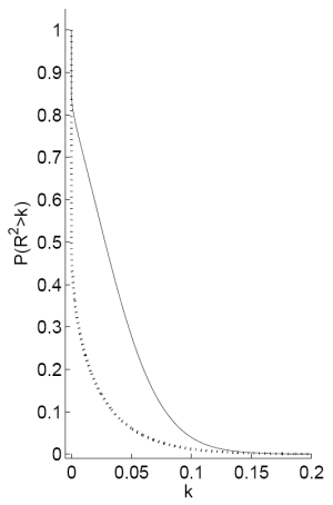
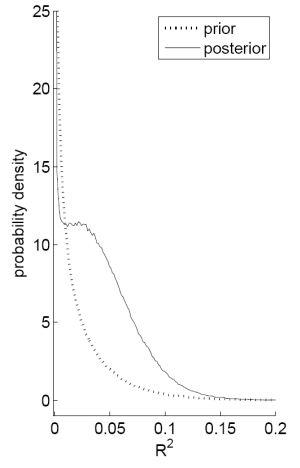
Figure C shows two plots on the prior and posterior distribution of the ![]() with priors
with priors
![]() and
and ![]() using the payout yield to predict
annual returns. Panel A plots
using the payout yield to predict
annual returns. Panel A plots
![]() as a function of
as a function of ![]() for both the prior and the posterior; this
corresponds to 1 minus the cumulative density function of the
for both the prior and the posterior; this
corresponds to 1 minus the cumulative density function of the ![]() .8 The plot for the
.8 The plot for the
![]() demonstrates a clear rightward shift for the posterior for values of
demonstrates a clear rightward shift for the posterior for values of ![]() up to 0.15 (both the prior and the posterior place similarly low probabilities that the
up to 0.15 (both the prior and the posterior place similarly low probabilities that the ![]() exceeds 0.15). The strength of the predictability can be seen in that while the
prior implies
exceeds 0.15). The strength of the predictability can be seen in that while the
prior implies
![]() , the posterior implies
, the posterior implies
![]() close to 0.85. Thus, after observing the data, an investor revises his beliefs on the strength of predictability substantially upward. Panel B plots the probability density
function of the
close to 0.85. Thus, after observing the data, an investor revises his beliefs on the strength of predictability substantially upward. Panel B plots the probability density
function of the ![]() . The full Bayes prior places the highest density on low values of the
. The full Bayes prior places the highest density on low values of the ![]() . The posterior however places high density in the region around 5% and has lower density than the prior for
. The posterior however places high density in the region around 5% and has lower density than the prior for ![]() values less than 2%. The evidence in favor of predictability,
with a moderate
values less than 2%. The evidence in favor of predictability,
with a moderate ![]() , is sufficient to overcome the investor's initial skepticism.
, is sufficient to overcome the investor's initial skepticism.
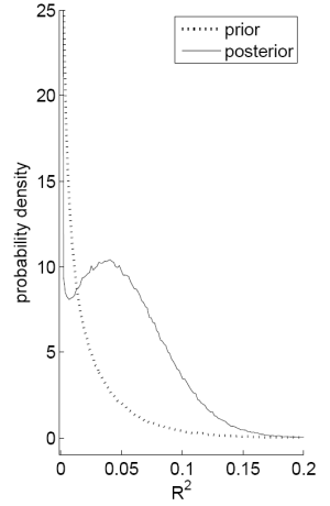
Figure C shows the comparable plots using the dividend-price ratio to predict annual returns. Results are similar to those discussed for the payout yield. The posterior probability of ![]() is again higher that the prior probability for
is again higher that the prior probability for ![]() ranging from 0 to 15%. The probability that the
ranging from 0 to 15%. The probability that the ![]() exceeds 1% goes from 15% to about 75%. The probability density function also shows lower density than the prior for very low values of the
exceeds 1% goes from 15% to about 75%. The probability density function also shows lower density than the prior for very low values of the ![]() and again places high density in the region of 5%.
and again places high density in the region of 5%.
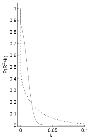
Figure C repeats this analysis using the dividend-price ratio to predict quarterly returns. The results show that the posterior clearly favors the existence of a moderate amount of predictability (note that we would expect the ![]() measured at a quarterly horizon to be below that for an annual horizon). Panel A shows that the probability that the
measured at a quarterly horizon to be below that for an annual horizon). Panel A shows that the probability that the ![]() exceeds 1% is 25% for the prior but above 80% for the posterior. More generally, the posterior probability that the
exceeds 1% is 25% for the prior but above 80% for the posterior. More generally, the posterior probability that the ![]() exceeds
exceeds ![]() is greater for the posterior than for the prior for all
is greater for the posterior than for the prior for all ![]() . Panel B shows that the posterior density exhibits a
clear spike around
. Panel B shows that the posterior density exhibits a
clear spike around ![]() .
.
The above analysis evaluates the statistical evidence on predictability. The Bayesian approach also enables us to study the economic gains from market timing. In particular, we can evaluate the certainty equivalent loss from failing to time the market under different priors on the existence and strength of predictability.
3.5 Certainty equivalent returns
We now measure the economic significance of the predictability evidence using certainty equivalent returns. We assume an investor who maximizes
![\displaystyle E\left[\left.\frac{W_{T+1}^{1-\gamma}}{1-\gamma} \right\vert D\right]](img136.gif)
 |
for
A draw ![]() from the distribution
from the distribution
![]() is given by (1) with probability
is given by (1) with probability ![]() and (2) with probability
and (2) with probability ![]() . The posterior distribution of the parameters is described in Section 2.4.
. The posterior distribution of the parameters is described in Section 2.4.
For any portfolio weight ![]() , we can compute the certainty equivalent return as solving
, we can compute the certainty equivalent return as solving
![\displaystyle \frac{\exp\left\{(1-\gamma)\mbox{CER}\right\}}{1-\gamma} = E\left[\left.\frac{(w\exp\{r_{T+1}+r_{f,T}\} + (1-w)\exp\{r_{f,T}\})^{1-\gamma}}{1-\gamma} \right\vert D\right].](img146.gif)
Following Kandel and Stambaugh (1996), we measure utility loss as the difference between certainty equivalent returns from following the optimal strategy and from following a sub-optimal strategy. We define the sub-optimal strategy as the strategy that the investor would follow if he believes that there is no predictability. Note, however, that the expectation in (31) is computed with respect to the same distribution for both the optimal and sub-optimal strategy.
Table 5 presents the average certainty equivalent loss: we compute the difference in certainty equivalent returns as described above, and then average over the posterior distribution for ![]() . The data indicate economically meaningful economic losses from failing to time the market. Panel A shows that, for example, an investor with a prior on
. The data indicate economically meaningful economic losses from failing to time the market. Panel A shows that, for example, an investor with a prior on ![]() such that
such that
![]() and a 50% prior belief in the existence of return predictability would suffer a certainty equivalent loss of
and a 50% prior belief in the existence of return predictability would suffer a certainty equivalent loss of ![]() from failing to time the market using the payout yield.9 Higher values of
from failing to time the market using the payout yield.9 Higher values of ![]() imply greater certainty equivalent losses. Panel B shows somewhat lower certainty equivalent losses for the dividend-price ratio using annual data. However, the certainty equivalent loss is much greater for
distributions computed using quarterly postwar data: 1.83% per annum for the investor with
imply greater certainty equivalent losses. Panel B shows somewhat lower certainty equivalent losses for the dividend-price ratio using annual data. However, the certainty equivalent loss is much greater for
distributions computed using quarterly postwar data: 1.83% per annum for the investor with
![]() , and
, and ![]() , and higher for higher levels of
, and higher for higher levels of ![]() .
.
4 Conclusion
This study has taken a Bayesian model selection approach to the question of whether the equity premium varies over time. We considered investors who face uncertainty both over whether predictability exists, and over the strength of predictability if it does exist. We found substantial evidence in favor of predictability when the dividend-price ratio and payout yield were used to predict returns. Moreover, we found large certainty equivalent losses from failing to time the market, even for investors who have strong prior beliefs in a constant equity premium.
Finally, we found that taking a fully Bayesian approach that incorporates the exact likelihood function leads to substantially different inference as compared with empirical Bayes or the conditional likelihood function. Empirical Bayes tends to overstate the evidence in favor of predictability while using the conditional likelihood understates the evidence. These results point to the importance of taking into account the stochastic nature of the regressor when studying return predictability from a Bayesian perspective.
Appendix
A. Jeffreys prior under
Jeffreys argues that a reasonable property of a "no-information" prior is that inference be invariant to one-to-one transformations of the parameter space. Given a set of parameters ![]() , data
, data ![]() , and a log-likelihood
, and a log-likelihood ![]() , Jeffreys shows that
invariance is equivalent to specifying a prior as
, Jeffreys shows that
invariance is equivalent to specifying a prior as
Besides invariance, this formulation of the prior has other advantages such as minimizing asymptotic bias and generating confidence sets that are similar to their classical counterparts (see Phillips (1991)).
Our derivation for the limiting Jeffreys prior on
![]() follows Stambaugh (1999). (Zellner, 1996, pp. 216-220) derives a limiting Jeffreys prior by applying (1)
to the likelihood (24) and retaining terms of the highest order in
follows Stambaugh (1999). (Zellner, 1996, pp. 216-220) derives a limiting Jeffreys prior by applying (1)
to the likelihood (24) and retaining terms of the highest order in ![]() . Stambaugh shows that Zellner's approach is equivalent to applying (1)
to the conditional likelihood (23), and taking the expectation in (1) assuming that
. Stambaugh shows that Zellner's approach is equivalent to applying (1)
to the conditional likelihood (23), and taking the expectation in (1) assuming that ![]() is multivariate normal with mean (6) and variance (7). We adopt this approach.
is multivariate normal with mean (6) and variance (7). We adopt this approach.
We derive the prior density for
![]() and then transform this into the density for
and then transform this into the density for
![]() using the Jacobian. Let
using the Jacobian. Let
denote the natural log of the conditional likelihood. Let
![\displaystyle p(b_0,\Sigma^{-1}\vert H_0) \propto \left\vert-E\left[\begin{array}{cc} \frac{\partial^2 l_0}{\partial b_0\partial b_0^\top} & \frac{\partial^2 l_0}{\partial b_0\partial \zeta^\top } \frac{\partial^2 l_0}{\partial \zeta\partial b_0^\top} & \frac{\partial^2 l_0}{\partial \zeta\partial \zeta^\top} \end{array}\right] \right\vert^{1/2}.](img161.gif)
The the form of the conditional likelihood implies that
It follows from (4) that
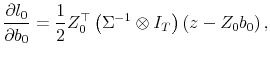

![\displaystyle -\frac{1}{2} \left[\begin{array}{cc} \iota_T^\top & 0 0 & X^\top \end{array}\right] \left(\Sigma^{-1}\otimes I_T\right) \left[\begin{array}{cc} \iota_T & 0 0 & X \end{array}\right]](img166.gif)
![\displaystyle -\frac{1}{2} \left[\begin{array}{cc} \sigma^{(11)}T & \sigma^{(12)}\iota^\top X \sigma^{(12)} X^\top \iota & \sigma^{(22)} X^\top X \end{array}\right].](img167.gif)
Taking the expectation conditional on
![\displaystyle E\left[\frac{\partial^2 l_0}{\partial b_0\partial b_0^\top} \right] = -\frac{T}{2}\left[\begin{array}{cc} \sigma^{(11)} & \sigma^{(12)} [1 \mu_x] \sigma^{(12)} \left[\begin{array}{c} 1 \mu_x \end{array}\right] & \sigma^{(22)} \left[\begin{array}{cc} 1 & \mu_x \mu_x & \sigma_x^2 + \mu_x^2 \end{array}\right] \end{array}\right]](img168.gif)
Using arguments in Stambaugh (1999), it can be shown that
![\displaystyle E\left[\frac{\partial^2 l_0}{\partial b_0\partial \zeta^\top}\right] = 0.](img169.gif)
where
![\displaystyle \Phi = \left[\begin{array}{cc} \Sigma^{-1} & \mu_x\left[\begin{array}{c} \sigma^{(12)} \sigma^{(22)} \end{array}\right] \mu_x \left[\sigma^{(12)} \sigma^{(22)}\right] & \left( \sigma_x^2 + \mu_x^2\right) \sigma^{(22)} \end{array}\right].](img172.gif)
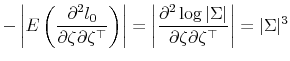
From the formula for the determinant of a partitioned matrix, it follows that
![\displaystyle \left\vert\Sigma^{-1} \right\vert \left\vert \left(\sigma_x^2 +\mu_x^2\right) \sigma^{(22)} - \mu_x^2 \left[\sigma^{(12)} \sigma^{(22)}\right]\Sigma \left[\begin{array}{c} \sigma^{(12)} \sigma^{(22)} \end{array}\right] \right\vert.](img176.gif) |
Because
![\displaystyle \Sigma\left[\begin{array}{c} \sigma^{(12)} \sigma^{(22)} \end{array}\right] = \left[\begin{array}{c} 0 1 \end{array}\right],](img177.gif)
The determinant of
Substituting into (7),
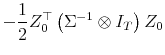
B. Sampling from Posterior Distributions
This section describes how to sample from the posterior distributions. In all cases, the sampling procedure for the posteriors under ![]() and
and ![]() involve the Metropolis-Hastings algorithm. Below we describe the case of the full Bayes exact likelihood in detail. The procedures for the other cases are similar.
involve the Metropolis-Hastings algorithm. Below we describe the case of the full Bayes exact likelihood in detail. The procedures for the other cases are similar.
B..1 Posterior distribution under
Substituting (8) and (24) into (25) implies that

The Metropolis-Hastings algorithm is implemented "block-at-a-time", by repeatedly sampling from
![]() and from
and from
![]() and repeating. To calculate a proposal density for
and repeating. To calculate a proposal density for ![]() , note that
, note that
![\begin{displaymath} B_0 = \left[ \begin{array}{cc} \alpha & \theta \ 0 & \rho\end{array}\right]. \end{displaymath}](img191.gif)
 proposal
Let
Let
 proposal
B..2 Posterior distribution under
Substituting (12) and (22) into (26) implies that
The sampling procedure is similar to that described in Appendix B.1. Details can be found in Wachter and Warusawitharana (2009). To summarize, we first draw from the posterior
![\begin{displaymath} B_1 = \left[ \begin{array}{cc} \alpha & \theta \ \beta & \rho\end{array}\right]. \end{displaymath}](img207.gif)
C. Computing the Bayes factor
Verdinelli and Wasserman (1995) provide an implementable formula for the inverse of the Bayes factor. In our notation, this formula can be written as
![\displaystyle \mathcal{B}_{10}^{-1} = p(\beta = 0 \vert H_1, D) E\left[\left.\frac{p(b_0, \Sigma \vert H_0)}{p(\beta = 0, b_0, \Sigma \vert H_1)} \right\vert \beta = 0, H_1, D\right].](img210.gif)
To compute
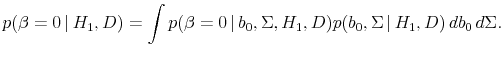
As discussed in Appendix B.2, the posterior distribution of
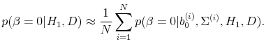
To compute the second term in (1), we observe that
because
Given these draws from the posterior distribution, the second term equals
![\displaystyle E\left[\left.\frac{p(b_0, \Sigma \vert H_0)}{p(\beta = 0, b_0, \Sigma \vert H_1)} \right\vert \beta = 0, H_1, D\right] \approx \frac{1}{N} \sum_{i=1}^N \sqrt{2 \pi} \sigma_{\eta} (\sigma_x^{(i)})^{-1} \sigma_u^{(i)},](img232.gif) |
(C.3) |
where this approximation is accurate for
Bibliography
"Should investors avoid all actively managed mutual funds? A study in Bayesian performance evaluation," The Journal of Finance, 56(1), 45-86. "Investing for the long run when returns are predictable," Journal of Finance, 55, 225-264. "Comment on 'A Statistical Paradox' by D. V. Lindley," Biometrika, 44, 533-534. Statistical decision theory and Bayesian analysis. Springer, New York. "On the importance of measuring payout yield: Implications for empirical asset pricing," Journal of Finance, 62(2), 877-915. Bayesian Inference in Statistical Analysis. Addison-Wesley Pub. Co., Reading, MA. "A simulation approach to dynamics portfolio choice with an application to learning about return predictability," Review of Financial Studies, 18, 831-873.
Notes: The figures plot the prior probability that the ![]() will be greater than some value
will be greater than some value ![]() for different values of
for different values of ![]() . This equals 1 minus the cumulative density function for the distribution on the
. This equals 1 minus the cumulative density function for the distribution on the ![]() . Panel A reports the values conditional on predictability
. Panel A reports the values conditional on predictability ![]() and panel B plots the values for a prior value of
and panel B plots the values for a prior value of ![]() .
.
![]() parameterizes the prior variance of
parameterizes the prior variance of ![]() with
with
![]() .
.
Notes: Panel A plots the probability that the ![]() from a predictive regression of excess stock returns on the payout yield will be greater than some value
from a predictive regression of excess stock returns on the payout yield will be greater than some value ![]() for different values of
for different values of ![]() . This equals 1 minus the cumulative density function for the distribution on the
. This equals 1 minus the cumulative density function for the distribution on the
![]() . Panel B plots the probability density function of the
. Panel B plots the probability density function of the ![]() for the same
regression. The dashed line signifies the prior and the solid line signifies the posterior distribution for the
for the same
regression. The dashed line signifies the prior and the solid line signifies the posterior distribution for the ![]() . The likelihood function for these plots is the full Bayes exact likelihood
with
. The likelihood function for these plots is the full Bayes exact likelihood
with
![]() and
and ![]() . Data are annual from 1/1/1927 to
1/1/2004.
. Data are annual from 1/1/1927 to
1/1/2004.
Notes: Panel A plots the probability that the ![]() from a predictive regression of excess stock returns on the dividend-price ratio will be greater than some value
from a predictive regression of excess stock returns on the dividend-price ratio will be greater than some value ![]() for different values of
for different values of ![]() . This equals 1 minus the cumulative density function for the
distribution on the
. This equals 1 minus the cumulative density function for the
distribution on the ![]() . Panel B plots the probability density function of the
. Panel B plots the probability density function of the ![]() for the same regression. The dashed line signifies the prior and the solid line signifies the posterior distribution for the
for the same regression. The dashed line signifies the prior and the solid line signifies the posterior distribution for the ![]() . The likelihood function for these plots is the full Bayes
exact likelihood with
. The likelihood function for these plots is the full Bayes
exact likelihood with
![]() and
and ![]() . Data are annual from 1/1/1927 to
1/1/2004.
. Data are annual from 1/1/1927 to
1/1/2004.
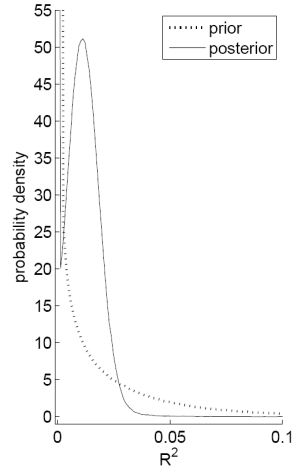
Notes: Panel A plots the probability that the ![]() from a predictive regression of excess stock returns on the dividend-price ratio will be greater than some value
from a predictive regression of excess stock returns on the dividend-price ratio will be greater than some value ![]() for different values of
for different values of ![]() . This equals 1 minus the cumulative density function for the
distribution on the
. This equals 1 minus the cumulative density function for the
distribution on the ![]() . Panel B plots the probability density function of the
. Panel B plots the probability density function of the ![]() for the same regression. The dashed line signifies the prior and the solid line signifies the posterior distribution for the
for the same regression. The dashed line signifies the prior and the solid line signifies the posterior distribution for the ![]() . The likelihood function for these plots is the full Bayes
exact likelihood with
. The likelihood function for these plots is the full Bayes
exact likelihood with
![]() and
and ![]() . Data are quarterly from 4/1/1952
to 1/1/2005.
. Data are quarterly from 4/1/1952
to 1/1/2005.
| Model: |
|
|
|
||
|---|---|---|---|---|---|
| Full Bayes, Exact Likelihood: 0.05 | 1.68 | 2.23 | 0.936 | 5.24 | -3.17 |
| Full Bayes, Exact Likelihood: 0.50 | 11.99 | 12.94 | 0.889 | 5.14 | -3.16 |
| Full Bayes, Exact Likelihood: 0.99 | 18.20 | 19.54 | 0.878 | 5.05 | -3.16 |
| Full Bayes, Conditional Likelihood: 0.05 | 1.36 | 1.39 | 0.959 | 5.64 | -5.32 |
| Full Bayes, Conditional Likelihood: 0.50 | 5.51 | 10.71 | 0.910 | 4.87 | -3.76 |
| Full Bayes, Conditional Likelihood: 0.99 | 6.54 | 16.42 | 0.914 | -22.66 | -6.24 |
| Empirical Bayes, Exact Likelihood: 0.05 | 2.58 | 3.99 | 0.926 | 5.22 | -3.17 |
| Empirical Bayes, Exact Likelihood: 0.50 | 19.43 | 14.17 | 0.887 | 5.13 | -3.16 |
| Empirical Bayes, Exact Likelihood: 0.99 | 27.13 | 21.90 | 0.851 | 5.09 | -3.16 |
| OLS | 20.89 | 0.863 | 5.85 | -3.15 |
| Model: |
|
|
|
||
|---|---|---|---|---|---|
| Full Bayes, Exact Likelihood: 0.05 | 1.51 | 1.48 | 0.966 | 4.71 | -3.37 |
| Full Bayes, Exact Likelihood: 0.50 | 5.73 | 7.64 | 0.946 | 4.37 | -3.35 |
| Full Bayes, Exact Likelihood: 0.99 | 6.90 | 11.30 | 0.948 | 4.02 | -3.35 |
| Full Bayes, Conditional Likelihood: 0.05 | 1.21 | 0.83 | 0.980 | 5.31 | -10.24 |
| Full Bayes, Conditional Likelihood: 0.50 | 2.78 | 5.56 | 0.963 | 3.15 | -6.75 |
| Full Bayes, Conditional Likelihood: 0.99 | 3.53 | 8.90 | 0.976 | -83.53 | -16.17 |
| Empirical Bayes, Exact Likelihood: 0.05 | 2.23 | 2.65 | 0.960 | 4.64 | -3.36 |
| Empirical Bayes, Exact Likelihood: 0.50 | 9.17 | 8.85 | 0.942 | 4.31 | -3.34 |
| Empirical Bayes, Exact Likelihood: 0.99 | 9.00 | 13.28 | 0.925 | 4.17 | -3.33 |
| OLS | 11.64 | 0.944 | 5.85 | -3.27 |
| Model |
|
|
|
||
|---|---|---|---|---|---|
| Full Bayes, Exact Likelihood: 0.05 | 4.68 | 1.05 | 0.990 | 3.20 | -3.49 |
| Full Bayes, Exact Likelihood: 0.50 | 7.06 | 1.87 | 0.984 | 3.21 | -3.50 |
| Full Bayes, Exact Likelihood: 0.99 | 6.48 | 2.01 | 0.983 | 3.21 | -3.50 |
| Full Bayes, Conditional Likelihood: 0.05 | 2.14 | 0.69 | 0.994 | 2.68 | -8.13 |
| Full Bayes, Conditional Likelihood: 0.50 | 2.90 | 1.51 | 0.988 | 0.53 | -6.87 |
| Full Bayes, Conditional Likelihood: 0.99 | 2.59 | 1.59 | 0.988 | -4.74 | -8.66 |
| Empirical Bayes, Exact Likelihood: 0.05 | 10.57 | 1.44 | 0.988 | 3.20 | -3.50 |
| Empirical Bayes, Exact Likelihood: 0.50 | 11.72 | 2.43 | 0.979 | 3.20 | -3.50 |
| Empirical Bayes, Exact Likelihood: 0.99 | 9.34 | 2.77 | 0.976 | 3.20 | -3.50 |
| OLS | 2.74 | 0.976 | 5.22 | -3.51 |
| Predictor
|
Prior prob. of return predictability |
Prior prob. of return predictability |
Prior prob. of return predictability |
Prior prob. of return predictability |
|---|---|---|---|---|
| Payout Yield, Annual Data: 0.05 | 0.02 | 0.30 | 0.63 | 0.87 |
| Payout Yield, Annual Data: 0.50 | 0.11 | 0.75 | 0.92 | 0.98 |
| Payout Yield, Annual Data: 0.99 | 0.16 | 0.82 | 0.95 | 0.99 |
| Dividend-Price Ratio, Annual Data: 0.05 | 0.02 | 0.27 | 0.60 | 0.86 |
| Dividend-Price Ratio, Annual Data: 0.50 | 0.05 | 0.59 | 0.85 | 0.96 |
| Dividend-Price Ratio, Annual Data: 0.99 | 0.07 | 0.63 | 0.87 | 0.97 |
| Dividend-Price Ratio, Quarterly Data: 0.05 | 0.05 | 0.54 | 0.82 | 0.95 |
| Dividend-Price Ratio, Quarterly Data: 0.50 | 0.07 | 0.64 | 0.88 | 0.97 |
| Dividend-Price Ratio, Quarterly Data: 0.99 | 0.06 | 0.62 | 0.87 | 0.96 |
| Predictor
|
Prior prob. of return predictability |
Prior prob. of return predictability |
Prior prob. of return predictability |
Prior prob. of return predictability |
|---|---|---|---|---|
| Payout Yield, Annual Data: 0.05 | 0.01 | 0.03 | 0.05 | 0.07 |
| Payout Yield, Annual Data: 0.50 | 0.57 | 0.82 | 0.92 | 0.95 |
| Payout Yield, Annual Data: 0.99 | 1.15 | 1.50 | 1.61 | 1.65 |
| Dividend-Price Ratio, Annual Data: 0.05 | 0.01 | 0.03 | 0.06 | 0.08 |
| Dividend-Price Ratio, Annual Data: 0.50 | 0.37 | 0.69 | 0.84 | 0.90 |
| Dividend-Price Ratio, Annual Data: 0.99 | 0.97 | 1.60 | 1.87 | 1.98 |
| Dividend-Price Ratio, Quarterly Data: 0.05 | 0.42 | 0.86 | 1.07 | 1.16 |
| Dividend-Price Ratio, Quarterly Data: 0.50 | 1.14 | 1.83 | 2.11 | 2.21 |
| Dividend-Price Ratio, Quarterly Data: 0.99 | 1.19 | 1.97 | 2.30 | 2.42 |
Footnotes
![\displaystyle E[r\vert D,H_1] = E\left[\alpha + \beta \frac{\theta}{1-\rho}\vert H_1\right],](img123.gif)