
Credit Card Redlining Revisited
Keywords: Credit cards, redlining, racial disparities, discrimination
Abstract:
1 Introduction
Using a proprietary database of credit bureau records, Cohen-Cole (2008) finds that lenders set credit limits on revolving accounts based in part on the racial composition of the neighborhood in which a borrower resides. Specifically, the author concludes that "it appears likely that a race variable appears somewhere in the determination of credit availability" (p. 1). This is a serious charge, as using the racial composition of a borrower's neighborhood to establish credit limits on revolving accounts would be a clear violation of the Equal Credit Opportunity Act (ECOA).
This paper uses the same proprietary database of credit bureau records to attempt to replicate the findings in that working paper. This replication attempt reveals three things. First, the summary statistics reported for the credit score variable are inconsistent both with the replicated dataset and with the dataset from which the author's data were originally drawn. The reported coefficients on this variable are also inconsistent with the estimation results from the replicated dataset. Second, the more than 135,000 observations (about 23 percent of the available sample) to which the author assigns missing values for the available credit measure because of "gaps in the original data" (p. 6), instead, appear to result from an undocumented decision about how to construct that variable. Third, the method used to calculate values for neighborhood demographic characteristics appears to unnecessarily exclude over 40,000 individuals, residing primarily in rural areas or areas bordering large bodies of water, from the estimation samples. Together, in the baseline estimation of available credit, these items are found to have increased the size of the effect reported in that paper by over 25 percent.
Beyond the replication, this paper also explores the robustness of the results in that working paper. When a variable measuring neighborhood income is added to the estimations, the results presented as evidence of redlining disappear. While the author of the earlier study finds that moving an individual from an 80% majority white to an 80% majority black area2 reduces credit by an average of $7,357, I find that when neighborhood income is controlled for, such a move appears to increase credit by a statistically insignificant $207. These results appear inconsistent with a finding of "uniformly lower access to credit in Black communities" (p. 14).
While this analysis suggests that the conclusions reached by Cohen-Cole (2008) are problematic, it nonetheless does not suggest that revolving credit is being allocated without regard to race or ethnicity. There are several reasons to suspect that the ability of the econometric approach to identify redlining activities is limited. Foremost among these reasons are (1) the implausibility of the assumption that aggregate credit limits, which are clearly affected by the number of credit accounts an individual chooses to maintain, reflect solely supply decisions and not demand factors; and (2) the endogeneity arising from regressing contemporaneous credit scores on credit limits or balances, which are themselves inputs used to calculate these scores. These issues with the identification strategy are discussed in more detail later in this paper.
The remainder of this paper presents my analysis of the findings of Cohen-Cole (2008). The next section discusses the data used and examines how decisions about variable construction affected the size of the samples used in the estimations reported in that paper. The following section then presents the replication of the estimations and examines the robustness of the results to the inclusion of a control for neighborhood income. Finally, the last section concludes by highlighting some issues involving the identification strategy.
2 Data and Variable Creation
The data used by Cohen-Cole ("CC," 2008) in his analysis of revolving credit patterns come from a nationally representative sample of individual-level credit bureau records. These data were supplied to CC by staff of the Federal Reserve Board, with the consent of the credit bureau. Because I have access to the original dataset that he received, an attempt to replicate CC's results is possible.
CC's findings are based on a series of estimations involving three different dependent variables summarizing each individual's revolving credit accounts. The first variable is utilization (UTIL), which measures the aggregate balances a person maintains on all of her revolving accounts. This measure is used to represent demand. The remaining two variables are used to measure supply. The first of these is credit limit (LIMIT), which captures the size of the aggregate credit lines on all of an individual's revolving accounts. When the credit limit on an account is not reported, the highest balance ever on that account is used in its place.3 The second supply measure is available credit (AVAILCREDIT), which represents the portion of a person's aggregate credit lines that are not used; that is, it is the difference between LIMIT and UTIL.
Each of the two supply measures, AVAILCREDIT and LIMIT, is modeled as a function of a contemporaneous credit score and the racial composition of an individual's neighborhood. Differences in LIMIT or AVAILCREDIT across neighborhoods with varying racial compositions, after controlling for credit scores and other factors, are attributed to redlining by revolving credit issuers. As a robustness check, additional information is added to the estimations, including each person's age from the credit bureau data, and a series of neighborhood characteristics calculated based on Census Bureau data and data drawn from the Federal Bureau of Investigation's Uniform Crime Reports.
Table 1 provides various summary statistics of the variables used in these estimations. The first column reproduces the means and medians reported by CC and the second column provides the same statistics from the replicated dataset. A comparison of the two columns suggests that the replicated dataset is very close to the one used by CC. Summary statistics for variables derived from Census Bureau or Uniform Crime Reports data are generally very similar and those based on data from the credit bureau match the reported results exactly, with one exception.
The exception is the credit score. The mean and median credit scores reported by CC are more than 40 points below those in the replicated sample. Because I do not have access to CC's computer code, the source of this difference cannot be determined. Nevertheless there are two reasons to suspect that that the reported values may be in error. First, the mean and median credit scores for the replicated sample exactly match those calculated from the dataset originally emailed to CC. Second, the median reported credit score is a decimal, whereas this credit score only takes on integer values.
Table 2 provides a count of the number of observations with missing values for the three variables that appear in the most parsimonious estimations. The first column reproduces the counts reported by CC and the second column lists the number of missing values in the replicated sample. While the counts of missing values for credit score and PCT_BLACK are very close to the reported numbers, counts of observations with missing values for AVAILCREDIT differ substantially. Despite this unexplained difference, the actual sample sizes used in the baseline estimations (shown in the bottom of table 2) are very similar.
As a result of missing values for these variables, over 200,000 observations are excluded from the estimations involving AVAILCREDIT, most of which are missing values for the dependent variable. The approximately 135,000 observations that are missing values for AVAILCREDIT (or 175,000 observations in the replicated dataset) are attributed by CC to "gaps in the original data" (p. 6). However, the original dataset contains no missing values. Instead, the missing values appear to be an artifact of the method used by the author to calculate AVAILCREDIT.
The original credit bureau data supplied to CC contain three pieces of information about the revolving accounts of each individual: aggregate balances, aggregate credit limits (using highest balance ever when the credit limit is unreported), and the utilization ratio. For unspecified reasons, the method of calculating AVAILCREDIT and UTIL adopted by CC makes no use of the measure of balances supplied by the credit bureau. Instead, it recalculates balances based upon the utilization ratio and aggregate credit limits. The use of this methodology appears to have two effects.
The first effect appears to result in almost all of the missing values. Individuals without revolving accounts have aggregate credit limits equal to zero and consequently their utilization ratios are undefined.4 These appear to be the observations that are assigned a missing value. Thus, the first effect of constructing UTIL and AVAILCREDIT this way appears to be the exclusion of individuals without revolving accounts from regressions involving either of these two variables, while leaving these observations in the estimations of LIMIT.
The second effect is subtler, but also appears to significantly affect the results. The variables supplied by the credit bureau are for purposes of constructing credit scoring models and occasionally use somewhat inconsistent definitions across variables. In this case, the definition a revolving account used in the calculation of the utilization ratio differs from that used to calculate aggregate credit limits or balances (which use identical definitions). The main difference is that revolving accounts with very large credit limits or outstanding balances are excluded from the calculation of the utilization ratio supplied by the credit bureau. 5 This difference is clearly observed in the data. Almost 1,000 observations have positive credit limits but undefined utilization ratios. The mean credit limit for these individuals is over $60,000 - approximately double the mean credit limit of individuals with positive utilization ratios. In contrast, there are no observations with reported utilization ratios and aggregate credit limits equal to zero.
The effect on AVAILCREDIT of using this methodology is shown in the upper panel of figure 1. The x-axis shows AVAILCREDIT calculated using the measure of balances and limits supplied by the credit bureau, both of which use consistent definitions of a revolving account. The y-axis shows the change in AVAILCREDIT that results from using balances calculated based on the utilization ratio, as done in CC. As the figure demonstrates, using the constructed measure of balances in the calculation of AVAILCREDIT, rather than the value supplied by the credit bureau, appears to increase AVAILCREDIT for people who have large unutilized credit lines. The bottom panel shows that the increase appears to be relatively smaller for individuals in high-minority concentration neighborhoods than for individuals in neighborhoods with lower minority concentrations. As will be shown in the next section, the decision to construct AVAILCREDIT using this methodology may have had an effect on the reported results.
Missing values for neighborhood racial composition, PCT_BLACK, may also have resulted in the exclusion of several thousand observations from each estimation. These missing values are correctly attributed by CC to "discrepancies between the geocodes from the credit bureau and the census" (p. 6). However, the discrepancies appear to be reconcilable and the assigned missing values may have been an unnecessary result of methodology used to define an individual's neighborhood. Under this methodology, an individual's neighborhood is comprised of all census block groups whose "internal points," as reported by the Census Bureau, are within 1 mile of the longitude and latitude coordinates for that individual in the credit bureau data. This methodology can lead to missing values in at least two specific circumstances.
The first circumstance involves individuals who reside in block groups or tracts on the coasts or near large bodies of water. While the longitude and latitude coordinates in the credit bureau data and the internal points provided in the Census data both generally coincide with geographic centroids,6 the Census internal points are constructed so that they always fall on land (U.S. Census Bureau, 2002). This leads to the problems depicted in figure 2. As shown in that figure, for block groups that encompass large bodies of water, the longitude and latitude coordinates reported in the bureau data may correspond to locations in the water. Since the internal points in the Census data must fall on land, the distance between the two points is frequently greater than 1 mile and the value for PCT_BLACK is set to missing. Consequently, people who live along the coasts, the Gulf of Mexico, or large rivers or lakes may be disproportionately excluded from the estimations.
The second circumstance affects a broader range of individuals. While both the credit bureau coordinates and Census internal points generally correspond to geographic centroids, the two points for a given block group are often quite different as can be seen in figure 2. The larger the geographic area spanned by the block group (or tract) the more likely it is that this difference will exceed 1 mile. When this happens, a missing value is assigned for PCT_BLACK, even when it is clear that both points are within the same block group. Since block groups tend to be geographically larger in more rural areas, missing values of PCT_BLACK should be more common in rural parts of the country.
This result is apparent in the data. In the replication sample, 48,001 observations out of 586,800, or about 8.2 percent, are assigned missing values for PCT_BLACK. In the 10 states with the lowest rural population shares according to the 2000 Census, 5.5% of observations have missing values for PCT_BLACK.7 In the 10 states with the highest rural population shares, PCT_BLACK was assigned a missing value in 18.8 percent of the cases.8 In the extreme case of Washington, DC, which has no rural population, there are no missing values for PCT_BLACK in the replication sample. The method of defining neighborhoods used by CC appears, therefore, to disproportionately exclude rural individuals and individuals who live near a major body of water.
Together, the methods used to represent balances and to define neighborhoods appear to account for most of the observations excluded from the estimation samples because of missing values.9 To examine the effects that these methods may have had on the reported results, I create a new "modified sample." In this sample, UTIL and AVAILCREDIT are calculated based upon the balances provided by the credit bureau, so that a consistent definition of a revolving account is used throughout. In addition, longitude and latitude coordinates are used, along with the FIPS codes provided by the credit bureau, to assign each individual to a block group, or where appropriate to a census tract.10 A one-mile radius around the internal point corresponding to that block group is then used to identify the other block groups that comprise the neighborhood in which the individual resides. The characteristics of these block groups are used to calculate values for PCT_BLACK and other Census-based variables.11
The number of missing values in the modified sample is shown in column 3 of table 2. The modified sample has no missing values for AVAILCREDIT and 53 observations with missing values for PCT_BLACK.12 Consequently, over 130,000 observations that had been assigned missing values can be included in the estimation. Summary statistics for the observations in this modified sample are given in column 4 of table 1. A comparison of this sample with the replicated sample (shown in column 3) reveals several differences. As expected, AVAILCREDIT is much smaller in the modified sample than in the replicated sample. This reflects both the inclusion of individuals with no revolving accounts and the elimination of the distortions introduced by using inconsistent definitions of a revolving account in calculating AVAILCREDIT. The modified sample also has higher neighborhood minority concentration levels and lower mean and median credit scores. This suggests that the methodology used to calculate AVAILCREDIT and PCT_BLACK may have eliminated a disproportionate number of individuals with low credit scores or who reside in neighborhoods with above-average minority concentrations.
3 Estimation Replication and Robustness Evaluation
In this section, replications of the equations estimated by CC are reported, using both the replicated sample and the modified sample described above. In addition, I evaluate the robustness of the results to the addition of a variable measuring neighborhood income. This income variable is constructed using the same 1-mile radius approach used to construct the other variables that are derived from Census data. It is also the same measure of neighborhood income used to construct the instruments, which are discussed in greater detail below.
CC reports results from three general specifications. The first specification involves single equation estimations of AVAILCREDIT and LIMIT that model these variables as linear functions of credit score and PCT_BLACK. The second specification is similar to the first, except that these estimations include an interaction term between PCT_BLACK and credit score, as well as additional control variables in some cases. As a result, the slope on PCT_BLACK can vary across individuals according to their credit score. The final specification uses instrumental variable techniques to estimate equations for LIMIT, while controlling for demand (as reflected by UTIL). In this section, we discuss the results of each general specification in turn.
3.1 Single Equation without Interaction Term Results
The first set of results presented by CC as evidence of redlining involves single equation estimations with either AVAILCREDIT or LIMIT as the dependent variable. Columns (1a) and (2a) of table 3 reproduce the coefficients reported by CC for these base models, using AVAILCREDIT and LIMIT respectively. The adjacent columns, (1b) and (2b), then present the coefficient values from identical estimations using the replicated dataset.
The replicated sample results are similar, but not identical to those reported by CC. In particular, the coefficients on credit score are lower in the replicated estimations than in the reported results. This is consistent with my earlier finding that the summary statistics for the credit score reported by CC are lower than the values in the replicated sample. Aside from this difference, the coefficients in the replicated estimation have magnitudes and statistical significance levels that are consistent with the reported results.
To evaluate how the two variable creation methods discussed earlier may have affected these results, identical estimations were conducted using the modified sample. The results of these estimations are provided in columns (1c) and (2c) of table 3. The modified sample sizes are significantly larger than the reported or replicated sample sizes. In the estimation of AVAILCREDIT, the coefficient on PCT_BLACK is substantially lower when the estimation is conducted on the modified sample than on the replicated sample. This suggests that the variable creation methods used by CC may have increased the size of the reported effect from this regression by 28.3 percent. In the single-equation estimation of LIMIT, which is unaffected by the methodology used to calculate balances, the reported effect is larger in the modified sample. Despite these differences in the sizes of the coefficients, the statistical significance levels of the coefficients remain consistent with those reported by CC.
To test how robust these results are to the inclusion of a control for neighborhood income, an additional series of estimations with a single slope was conducted. These estimations, the results of which are provided in columns (1d) and (2d) of table 3, include the same variables as in the previous three columns, plus an additional variable representing mean neighborhood income. When this control is added, the results that CC presents as evidence of redlining disappear. In the estimations for both AVAILCREDIT and LIMIT, the coefficient on PCT_BLACK goes from being negative and significant at the 1 percent level to being small and statistically insignificant. At the same time, the coefficient on neighborhood income is positive and significant at the 1 percent level in both estimations.
These results suggest that CC's findings are not robust to the inclusion of a control for neighborhood income. Furthermore, the conclusion that CC draws based upon the reported coefficients - that moving an individual from an 80% majority white neighborhood to one that is 80% majority black reduces credit by $7,357 - appears to be largely driven by differences in income across neighborhoods. When neighborhood income is held constant, moving an individual from an 80% majority white to an 80% majority black census tract appears to increase credit by $207, though this difference is not statistically significant.
3.2 Single Equation with Interaction Term Results
In addition to single equation estimations with a constant slope for PCT_BLACK, CC also estimates a large number of equations that include an interaction of PCT_BLACK and credit score. This interaction allows the effect of a neighborhood's racial composition to differ according to the credit score of the borrower.
In total, CC reports the results from 14 different single equation models with score-varying slopes. Unfortunately, I am unable to replicate any of the estimations that include variables for income. The reason is that in the limited number of estimations that include income (4 of the 14), income is always added in conjunction with other variables. One of these other variables is inflation-adjusted income growth, which CC states was calculated at the Public Use Microdata Area (PUMA) level based upon data from the American Community Survey (ACS) for 2000 and 2005. However, the 2000 ACS did not release data at the PUMA level, so it does not appear that the variable could have been constructed as reported.13 While I am therefore unable to attempt a replication of the results involving income variables, I can attempt to replicate the estimations that do not include the income growth variable.
Rather than reproduce results from all 10 of the replicated estimations, I focus here on the most parsimonious and the most comprehensive. These are provided in tables 4 and 5, respectively. Columns (1a) and (2a) in each table reproduce the results presented by CC and columns (1b) and (2b) provide my replication. Again, the replicated results appear similar, with the exception of a somewhat lower coefficient on credit score and different coefficients on property and violent crime rates. Differences in coefficients on the crime rates may be related to the unexplained fact that my replicated estimation used approximately 15,000 more observations than are reported by CC. Nevertheless, the coefficients of interest remain similar in size and statistical significance level to the reported results.
Columns (1c) and (2c) provide the estimation results based upon the modified sample and columns (1d) and (2d) present the modified sample results with the addition of a variable measuring neighborhood income. A comparison of these columns shows that the addition of the income variable has a similar effect in all four estimations; that is, the coefficient on PCT_BLACK becomes larger and the coefficient on the interaction term, SC_BLACK, becomes smaller. Similarly, the additional control variables included in the estimations in table 5 also result in a higher positive coefficient on PCT_BLACK and a smaller coefficient on SC_BLACK relative to those from the estimations in table 4.
These results are more difficult to interpret than those produced by the results with a single slope. The opposing signs on PCT_BLACK and SC_BLACK imply that there is some "break even" credit score below which individuals will be helped by redlining (that is, they will have higher credit limits than individuals with identical characteristics in all-white neighborhoods) and above which they will be harmed.
The existence or importance of this break even credit score is not mentioned by CC. Instead, he focuses on the fact that the "race penalty," or the difference between the amount of revolving credit the model predicts each person has and the amount the model predicts the person would have had in an all-white neighborhood, "is greater for individuals with better credit history scores" (p. 14). This statement is true in that the derivative of the race penalty with respect to credit score is always positive. However, this does not account for the fact that the race penalty may be negative at low credit score levels (so that borrowers with sufficiently low credit scores have higher credit limits than identical borrowers in all-white neighborhoods). Consequently, a positive derivative on the race penalty may mask the relationship between neighborhood racial composition and LIMIT or AVAILCREDIT.
For example, consider the parameter values from the estimation of AVAILCREDIT using the replicated sample, given in column 2 of table 5. These parameter values indicate that the break even credit score occurs around 627.14 While this level is below the mean credit score for the entire sample (647), mean credit scores are generally lower in neighborhoods with higher minority concentrations (Board of Governors, 2007). This relationship is also observed for the sample here, as demonstrated in figure 3. As that figure indicates, neighborhoods with disproportionally large minority concentrations generally have mean credit scores below this level, suggesting that, on average, individuals in neighborhoods with high minority concentrations may have higher credit limits than identical individuals in all-white neighborhoods.
This pattern is evident in the data. Using the estimated coefficients from each model, the race penalty is calculated for each individual in the sample as the difference between the amount of revolving credit the model predicts the person would have and the amount the person would have had in an all-white neighborhood. Panel (a) of figure 4 shows the mean race penalty for neighborhoods with different racial compositions using the estimations reported in column (1c) of table 5. As indicated in that graph, the race penalty for AVAILCREDIT is generally negative for majority black neighborhoods, suggesting that individuals in these neighborhoods had more available credit than similar individuals in all-white neighborhoods. This evidence appears to be inconsistent with CC's conclusion that an individual in a black neighborhood has less ability to access credit. When a control is added for neighborhood income, the estimated race penalty appears as shown in panel (b) of figure 4. As that graph (which is based upon the coefficients provided in column (1d) of table 5) shows, the mean race penalty is negative for almost all neighborhood racial composition levels. The patterns for the race penalty calculated using estimations of LIMIT, shown in panels (c) and (d) of figure 4, are very similar.
The results of the replication of the estimations involving SC_BLACK show that the evidence of systematically lower levels of AVAILCREDIT or LIMIT for individuals in high-minority areas seems to disappear when a control is added for mean neighborhood income. This is consistent with the results in the previous section that the results reported by CC are not robust to the inclusion of a control for neighborhood income.
Though I am unable to attempt a replication of any of CC's estimations that control for neighborhood income for the reasons described above, the pattern observed in the results here seems to be evident in CC's reported results as well. Based on the coefficients reported by CC, the break even credit scores occur at 684 for AVAILCREDIT and 666 for LIMIT in the most comprehensive single-equation estimations involving income. Given that the mean credit score in all-white neighborhoods is 672, and that mean credit scores decline monotonically as the minority population share in a neighborhood increases (as shown in figure 3), these coefficients would appear to generate values for the race penalty that are inconsistent with a finding of systematically lower levels of AVAILCREDIT or LIMIT in minority neighborhoods, once income is controlled for.
3.3 Instrumental Variable Estimation Results
In addition to the single equation estimations, a series of multiple-equation estimations for UTIL and LIMIT are also presented by CC. These estimations use instruments for demand that are premised on the importance of relatively higher income neighbors to an individual's own consumption. If an individual's consumption is affected by the consumption choices of her neighbors (a "keeping up with the Joneses" effect) then the income levels of neighbors might be correlated with credit utilization but not with the credit supply decisions of lenders.
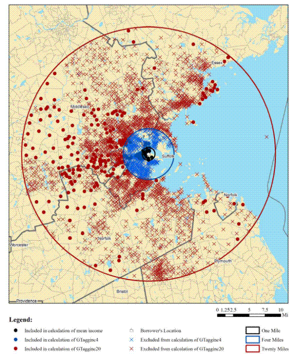
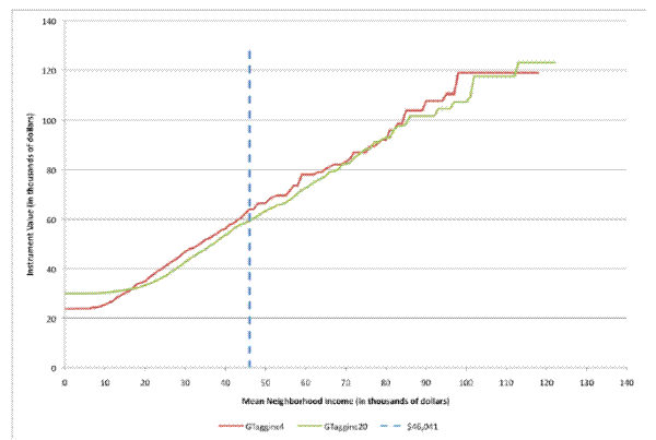
Motivated by this theory, CC creates two instruments based on mean incomes of census block groups located 1-4 miles and 4-20 miles away from each individual in the sample. An example of the construction of these instruments for a hypothetical person residing in Boston is provided by figure 5. The first step in the process is to identify all of the census block groups with internal points are that within 1 mile of the borrower (shown as the black circles in the figure) and to calculate the average income across these block groups. This measure of the mean neighborhood income, which in this example is equal to $46,041, is the same measure that I have been using in this paper. In the next step, all census block groups within 1 to 4 miles of the borrower with mean incomes that are greater than or equal to the borrower's neighborhood are identified and the mean income for individuals in these block groups is calculated. This value ($63,990) is the value for the first instrument, GTagginc4. The value for the second instrument, GTagginc20, is calculated identically, but using those block groups located from 4 to 20 miles away from the borrower with mean income levels above the mean income of the borrower's neighborhood.
The calculation of these two instruments, therefore, depends heavily on the mean income of the borrower's neighborhood. Figure 6 shows the value that each of the instruments would have taken in this example as a function of the borrower's neighborhood income. As this figure shows, the value of each instrument is highly related to neighborhood income, with the values of the instruments increasing as income increases. If neighborhood income is sufficiently large (above $118,817 or $122,938 for the two instruments, respectively) then all of the surrounding census block groups are excluded from the calculation and the value of the instrumental variable is treated as missing. Similarly, an instrument is assigned a missing value if there are no census block groups with internal points within either of the two radial bands. Missing values for one or both of the instruments appear to account for the exclusion of at least 30,000 observations from each of the instrumental variable estimations.
A strong relationship between the value of the instruments and the mean income of the local neighborhood is also apparent from the correlation between the variables. Both instruments have correlations with mean income in excess of 0.92. This suggests that the explanatory power of these instruments may derive primarily from their relationship with neighborhood income and not from efforts to keep up with the Joneses.
Table 6 provides the results of the instrumental variable regressions for the most parsimonious estimation. The table has the same four columns as earlier tables, depicting the results reported by CC, the results from the replicated sample, the results from the modified sample, and finally the results from the modified sample including a variable for mean income.
The results shown in this table appear to be consistent with the idea that these two instruments, while clever ideas, are operating primarily as proxies for neighborhood income. When mean income is excluded from the regressions, the coefficients on these instruments are consistently significant at the 1 percent level. However, when mean income is added, the coefficients on the instruments shrink substantially and lose their statistical significance. Furthermore, the Kleibergen-Paap LM test no longer rejects the null of underidentification (p-value=0.962).
Consequently, the appropriateness of these variables as instruments for demand is suspect. Proper instruments should be correlated with demand, but not supply and it would be difficult to argue that variables reflecting neighborhood income would meet this condition. The fact that CC includes neighborhood income variables in some of his estimations of AVAILCREDIT and LIMIT suggests that he would agree that neighborhood income does not meet the conditions to make it an appropriate instrument for demand.
Putting concerns about the validity of the instruments aside, the results reported by CC, and those generated by the replicated and modified samples, all include a coefficient on PCT_BLACK in the supply equation that is positive and significant at the 1 percent level. This implies that borrowers in high-minority areas have higher credit limits than otherwise identical borrowers in all-white neighborhoods. The sign on this coefficient is the opposite of what was found for the single equation estimations discussed earlier and it is unclear how to reconcile this with CC's statement that these coefficients are "similar in magnitude and sign" (p. 16) to the results reported in earlier estimations. The results of the instrumental variable regression with a single slope on PCT_BLACK appears inconsistent with a finding of reduced credit availability to high minority concentration neighborhoods.
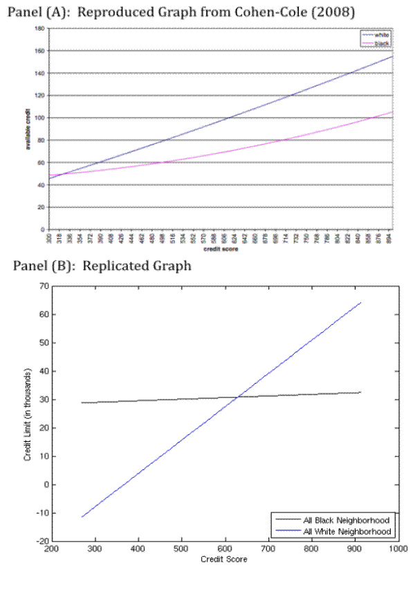
The remaining instrumental variable estimations include the same interaction term between credit score and PCT_BLACK that was discussed in the previous section. Again, these results are harder to interpret because they imply the existence of a break-even credit score, above which the race penalty is positive and below which it is negative. In discussing the instrumental variable results, CC presents the figure reproduced in the top panel of figure 7, which is attributed by CC to the reported estimation results presented in table 7 (along with the results from the replicated and modified samples). This figure shows that at low credit score levels "credit availability is quite low, but not distinguished greatly by race" (p. 16) and that, as credit scores increase, differences increase rapidly.
This figure appears to support a finding of systematically lower levels of credit in high minority neighborhoods. However, for several reasons, it is difficult to reconcile this figure with the reported coefficients upon which it is based. First, the graph shows AVAILCREDIT and not LIMIT, which is the dependent variable used in the instrumental variable estimations, as a function of credit score. Second, the break-even credit score is shown to be in the low 300s in the graph, while the coefficients imply that the break-even credit score should be closer to 632.15 Most importantly, however, the range of values spanned by the two curves in this graph run from a low of around $40,000 to almost $160,000 for the people with the highest credit scores living in all-white neighborhoods. Given that the sample averages for available credit ($23,267) and credit limits ($27,012) are both substantially below the bottom end of this range, it is unclear how to reconcile this graph with the estimations in CC's paper.
When using the replicated results for the estimation that generated this figure (provided in column (2b) of table 7), the graph appears as in the bottom panel of figure 7. This figure shows estimated aggregate credit limits by credit score level for an individual living in an all-white neighborhood and an individual living in an all-black neighborhood, with all other characteristics held constant at their sample means. Rather than exhibiting consistently higher levels of credit to borrowers in all-white neighborhoods at all but the lowest credit score levels, this figure shows a negative race penalty for individuals with scores below the break-even level and a positive race penalty for individuals with credit scores above that level. This break-even score is roughly consistent with the break-even levels observed in the previous section for the estimations using the modified sample with a control for neighborhood income. Consequently, the results of the instrumental variable estimations reported by CC and replicated here do not appear to support a finding of systematically lower credit levels in high minority areas.
4 Conclusions and Implications
This paper evaluates the evidence presented by Cohen-Cole (2008) that issuers of revolving credit set credit limits based upon the racial composition of the neighborhood in which a borrower resides. My attempt to replicate the results in that paper reveals three things. First, the reported summary statistics and estimated coefficients for the credit score variable are inconsistent with the results from the replicated dataset. The reported summary statistics for the credit score variable are also inconsistent with the dataset from which the author's data were originally drawn. Second, the more than 135,000 observations (representing 23 percent of the sample) that the author assigns missing values for the available credit measure because of "gaps in the original data" (p. 6), instead, appear to result from an undocumented decision about how to construct that variable. Third, the method used to calculate values for variables representing neighborhood demographic characteristics appears to unnecessarily exclude over 40,000 individuals (or approximately 7 percent of the sample), residing primarily in rural areas or areas bordering large bodies of water, from the estimation samples. Together, these items appear to have increased the size of the effect reported in the baseline estimation of available credit by over 25 percent.
As an additional robustness check, this paper also examines how the estimation results are impacted by the inclusion of a variable representing neighborhood income. The results show that, in each replicated estimation, the inclusion of such a control variable for neighborhood income causes the results presented as evidence of redlining to disappear. While the author of the earlier study finds that moving an individual from an 80% majority white to an 80% majority black area16 reduces credit by an average of $7,357, I find that when neighborhood income is controlled for, such a move appears to increase credit by a statistically insignificant $207. These results appear inconsistent with CC's finding of "uniformly lower access to credit in Black communities" (p. 14).
While this analysis suggests that the conclusions reached by CC are problematic, it would be premature to suggest that revolving credit is being allocated without regard to race or ethnicity. There are several reasons to suspect that the ability of the econometric approach to detect redlining activities is limited. Two reasons are particularly important.
The first reason is the implausibility of the assumptions underlying this econometric approach that: (1) aggregate credit limits or unused credit lines are measures of supply and (2) utilization solely represents demand. Given that AVAILCREDIT is defined as the difference between an individual's revolving balances and credit limits, an assumption that this variable solely captures supply is troublesome. If two individuals each get a credit card with the same limit, and one runs up charges equal to the credit limit while the other charges nothing, the value of AVAILCREDIT for these two individuals will be very different. This difference is unrelated to the supply decision of the lender. Consequently, the assumption that differences in AVAILCREDIT can be attributed solely to supply decisions is almost surely wrong.
Similar arguments can be made about the other two measures, UTIL and LIMIT. Aggregate credit limits will depend heavily on the number of credit cards or home equity lines a person chooses to maintain (subject, of course, to the willingness of lenders to extend credit), and this will depend upon both demand and supply effects (Gross and Souleles, 2002b).17 For example, an individual's decision to close a credit line will decrease aggregate credit lines, not as a result of a supply shock, but because of a decision made by the consumer. Likewise, balances maintained on revolving credit accounts will reflect both demand and supply considerations. Particularly for credit constrained individuals (such as individuals living in redlined neighborhoods where the provision of credit is kept low), the balances that are carried may be limited by the credit limits on open accounts and by the borrower's ability to obtain additional revolving accounts from other lenders. Consequently, balances and credit limits may reflect both demand and supply considerations and differences in aggregate credit limits across neighborhoods are unlikely to reflect decisions on the part of the lenders alone.
The second reason is the endogeneity inherent in using a contemporaneous credit score as a control variable. Rather than using an individual's credit score at the time the credit decision was made18, this econometric approach relies upon a credit score that is calculated on the same date as the dependent variables (utilization, credit limits, and available credit). Each of these dependent variables is an input into the calculation of a credit score.19 A contemporaneous credit score cannot be an exogenous predictor of utilization, credit limits, or available credit, if it is an endogenous function of these variables.
Specifically, two individuals with the same credit score, but substantially different credit limits20, must differ on the other characteristics that comprise a credit score (such as past delinquency). The Board of Governors of the Federal Reserve System (2007) has established that many of these other characteristics are correlated with both race and the racial composition of an individual's neighborhood. Finding a statistically significant coefficient on neighborhood racial composition, when controlling for a contemporaneous credit score, may reflect the correlation between neighborhood racial composition and the other factors that comprise the credit scoring model even in the absence of a causal link between credit limits and neighborhood racial compositions.21
Because of these issues with the econometric approach, it is very difficult to make definitive statements about whether issuers of revolving credit are engaging in redlining activities. Nevertheless, equal access to credit remains an important public policy issue. Practices, such as redlining, that limit credit availability for minorities or other demographic groups can have substantial negative consequences for the ability of individuals to establish credit histories, finance educations, own their own homes, or build wealth. Efforts aimed at detecting the existence of such practices represent valuable contributions not only to the literature, but also to furthering public policy goals. Whether issuers of revolving credit are engaging in redlining practices remains an open question that deserves serious study.
5 References
Avery, Robert B., Paul S. Calem, and Glenn B. Canner, 2004, "Credit Report Accuracy and Availability of Credit," Federal Reserve Bulletin, Summer, 90(3): pp. 297-322.
Board of Governors of the Federal Reserve System, 2007, Report to Congress on Credit Scoring and Its Effects on the Availability and Affordability of Credit.
Cohen-Cole, Ethan, 2008, "Credit Card Redlining." Federal Reserve Bank of Boston Working Paper No. QAU08-1.
Fair Isaac Corporation, 2007, Understanding Your FICO Score. Available at: http://www.myfico.com/Downloads/Files/myFICO_UYFS_Booklet.pdf (last visited May 8, 2008).
Gross, David B. and Nicholas S. Souleles, 2002a, "Do Liquity Constraints and Interest Rates Matter for Consumer Behavior? Evidence from Credit Card Data," The Quarterly Journal of Economics, February, 117(1): 149-85.
Gross, David B. and Nicholas S. Souleles, 2002b, "An Empirical Analysis of Personal Bankruptcy and Delinquency," The Review of Financial Studies, Spring, 15(1): 319-47.
Nelson, Charles, Edward Welniak, and Kirby G. Posey, 2003, "Income in the American Community Survey: Comparisons to Census 2000." Mimeo available at: http://www2.census.gov/acs/downloads/ASA_nelson.pdf (last visited April 23, 2009).
United States Bureau of the Census, 2002, Census 2000 Summary File 3 Technical Documentation.
| Reported Sample Statistics | Entire Replicated Sample | Replicated Estimation Sample | Modified Estimation Sample | |
|---|---|---|---|---|
| Credit Limit (LIMIT): Median | 6.100 | 6.100 | 18.640 | 10.900 |
| Credit Limit (LIMIT): Mean | 23.627 | 23.627 | 34.737 | 27.719 |
| Utilization: Median | 1.574 | 1.574 | 1.669 | 0.799 |
| Utilization: Mean | 6.582 | 6.582 | 6.783 | 7.714 |
| Available Credit (AVAILCREDIT): Median | 12.506 | 12.506 | 13.290 | 6.682 |
| Available Credit (AVAILCREDIT): Mean | 27.012 | 27.012 | 27.954 | 20.583 |
| Credit Score: Median | 652.851 | 700.000 | 753.000 | 700.000 |
| Credit Score: Mean | 606.351 | 647.732 | 693.778 | 647.770 |
| Age: Median | 46.000 | 46.000 | 47.000 | 46.000 |
| Age: Mean | 48.207 | 48.207 | 49.135 | 48.207 |
| Reported Sample Statistics | Entire Replicated Sample | Replicated Estimation Sample | Modified Estimation Sample | |
|---|---|---|---|---|
| Percent Black (PCT_BLACK): Median | 0.036 | 0.037 | 0.029 | 0.031 |
| Percent Black (PCT_BLACK): Mean | 0.127 | 0.128 | 0.102 | 0.113 |
| Violent Crime: Median | 0.004 | 0.004 | 0.004 | 0.004 |
| Violent Crime: Mean | 0.005 | 0.005 | 0.005 | 0.005 |
| Property Crime: Median | 0.033 | 0.034 | 0.033 | 0.033 |
| Property Crime: Mean | 0.036 | 0.037 | 0.036 | 0.036 |
| >HS ed - male: Median | 0.522 | 0.522 | 0.554 | 0.527 |
| >HS ed - male: Mean | 0.533 | 0.533 | 0.559 | 0.537 |
| >HS ed - female: Median | 0.504 | 0.504 | 0.529 | 0.510 |
| >HS ed - female: Mean | 0.515 | 0.515 | 0.536 | 0.520 |
| eq HS ed - male: Median | 0.269 | 0.269 | 0.263 | 0.274 |
| eq HS ed - male: Mean | 0.269 | 0.269 | 0.264 | 0.273 |
| eq HS ed - female: Median | 0.289 | 0.289 | 0.286 | 0.293 |
| eq HS ed - female: Mean | 0.290 | 0.290 | 0.287 | 0.293 |
| Public Assistance: Median | 0.024 | 0.024 | 0.021 | 0.023 |
| Public Assistance: Mean | 0.036 | 0.036 | 0.031 | 0.033 |
| Married Male: Median | 0.588 | 0.588 | 0.603 | 0.602 |
| Married Male: Mean | 0.580 | 0.580 | 0.593 | 0.592 |
| Married Female: Median | 0.540 | 0.540 | 0.553 | 0.555 |
| Married Female: Mean | 0.539 | 0.539 | 0.552 | 0.553 |
| Nonmarried Male: Median | 0.293 | 0.293 | 0.282 | 0.280 |
| Nonmarried Male: Mean | 0.307 | 0.307 | 0.297 | 0.297 |
| Nonmarried Female: Median | 0.227 | 0.227 | 0.219 | 0.217 |
| Nonmarried Female: Mean | 0.246 | 0.246 | 0.237 | 0.236 |
| Widowed Male: Median | 0.023 | 0.023 | 0.023 | 0.023 |
| Widowed Male: Mean | 0.026 | 0.026 | 0.025 | 0.025 |
| Widowed Female: Median | 0.100 | 0.110 | 0.107 | 0.107 |
| Widowed Female: Mean | 0.105 | 0.111 | 0.108 | 0.108 |
| Divorced Male: Median | 0.084 | 0.084 | 0.081 | 0.084 |
| Divorced Male: Mean | 0.088 | 0.088 | 0.085 | 0.086 |
| Divorced Female: Median | 0.110 | 0.100 | 0.099 | 0.100 |
| Divorced Female: Mean | 0.111 | 0.105 | 0.103 | 0.104 |
| Foreign Born: Median | 0.064 | 0.064 | 0.062 | 0.057 |
| Foreign Born: Mean | 0.116 | 0.116 | 0.111 | 0.011 |
| Reported Sample Statistics | Entire Replicated Sample | Replicated Estimation Sample | Modified Estimation Sample | |
|---|---|---|---|---|
| GTagginc4: Median | 26.161 | 26.391 | 27.674 | 26.648 |
| GTagginc5: Mean | 29.642 | 29.916 | 31.273 | 30.131 |
| GTagginc20: Median | 28.518 | 28.755 | 30.032 | 28.734 |
| GTagginc21: Mean | 31.438 | 31.698 | 32.965 | 31.610 |
| Reported Results | Replicated Sample | Modified Sample | |
|---|---|---|---|
| Total Observations | 586,800 | 586,800 | 586,800 |
| Missing Available Credit | 135,355 | 175,863 | 0 |
| Missing Percent Black | 48,065 | 48,001 | 53 |
| Missing Credit Score | 90,865 | 90,865 | 90,865 |
| Remaining Sample | 401,009 | 365,137 | 495,893 |
| Available Credit Sample Size | 365,092 | 365,137 | 495,893 |
| Credit Limit Sample Size | 454,692 | 454,749 | 495,893 |
| Dependent Variable: Available Credit (1a) Reported Results | Dependent Variable: Available Credit (1b) Replicated Sample | Dependent Variable: Available Credit (1c) Modified Sample | Dependent Variable: Available Credit (1d) Modified Sample | Dependent Variable: Credit Limit (2a) Reported Results | Dependent Variable: Credit Limit (2b) Replicated Sample | Dependent Variable: Credit Limit (2c) Modified Sample | Dependent Variable: Credit Limit (2d) Modified Sample |
|
|---|---|---|---|---|---|---|---|---|
| PCT_BLACK | -12.261*** | -12.370*** | -9.638*** | 0.346 | -13.419*** | -13.522*** | -15.137*** | 0.087 |
| PCT_BLACK Standard Error | (0.516) | (0.516) | (0.321) | (0.340) | (0.454) | (0.455) | (0.447) | (0.473) |
| Credit Score | 0.091*** | 0.081*** | 0.071*** | 0.067*** | 0.089*** | 0.080*** | 0.079*** | 0.074*** |
| Credit Score Standard Errors | (0.001) | (0.000) | (0.000) | (0.000) | (0.000) | (0.000) | (0.000) | (0.000) |
| Mean Income | 0.520*** | 0.793*** | ||||||
| Mean Income Standard Errors | (0.006) | (0.009) | ||||||
| Observations | 365,092 | 365,137 | 495,893 | 495,876 | 454,692 | 454,749 | 495,893 | 495,876 |
| R-squared | 0.082 | 0.082 | 0.137 | 0.149 | 0.094 | 0.094 | 0.094 | 0.110 |
| Dependent Variable: Available Credit (1a) Reported Results | Dependent Variable: Available Credit (1b) Replicated Sample | Dependent Variable: Available Credit (1c) Modified Sample | Dependent Variable: Available Credit (1d) Modified Sample | Dependent Variable: Credit Limit (2a) Reported Results | Dependent Variable: Credit Limit (2b) Replicated Sample | Dependent Variable: Credit Limit (2c) Modified Sample | Dependent Variable: Credit Limit (2d) Modified Sample |
|
|---|---|---|---|---|---|---|---|---|
| PCTBLACK | 13.105*** | 13.107*** | 15.534*** | 20.577*** | 7.070*** | 7.077*** | 8.045*** | 15.840*** |
| PCTBLACK Standard Errors | (1.498) | (1.497) | (0.774) | (0.771) | (1.112) | (1.112) | (1.077) | (1.071) |
| Credit Score | 0.097*** | 0.086*** | 0.076*** | 0.072*** | 0.095*** | 0.084*** | 0.084*** | 0.077*** |
| Credit Score Standard Errors | (0.001) | (0.001) | (0.000) | (0.000) | (0.001) | (0.000) | (0.000) | (0.000) |
| SC_BLACK | -0.041*** | -0.041*** | -0.046*** | -0.038*** | -0.037*** | -0.037*** | -0.043*** | -0.029*** |
| SC_BLACK Standard Errors | (0.002) | (0.002) | (0.001) | (0.001) | (0.002) | (0.002) | (0.002) | (0.002) |
| Mean Income | 0.505*** | 0.781*** | ||||||
| Mean Income Standard Errors | (0.006) | (0.009) | ||||||
| Observations | 365,092 | 365,137 | 495,893 | 495,876 | 454,692 | 454,749 | 495,893 | 495,876 |
| R-squared | 0.083 | 0.083 | 0.139 | 0.150 | 0.094 | 0.094 | 0.095 | 0.110 |
| Dependent Variable: Available Credit (1a) Reported Results | Dependent Variable: Available Credit (1b) Replicated Sample | Dependent Variable: Available Credit (1c) Modified Sample | Dependent Variable: Available Credit (1d) Modified Sample | Dependent Variable: Credit Limit (2a) Reported Results | Dependent Variable: Credit Limit (2b) Replicated Sample | Dependent Variable: Credit Limit (2c) Modified Sample | Dependent Variable: Credit Limit (2d) Modified Sample |
|
|---|---|---|---|---|---|---|---|---|
| PCT_BLACK | 19.059*** | 18.801*** | 20.484*** | 22.133*** | 12.503*** | 12.542*** | 14.494*** | 17.266*** |
| PCT_BLACK Standard Errors | (1.707) | (1.659) | (0.926) | (0.925) | (1.391) | (1.352) | (1.308) | (1.306) |
| Credit Score | 0.095*** | 0.085*** | 0.076*** | 0.075*** | 0.093*** | 0.083*** | 0.081*** | 0.081*** |
| Credit Score Standard Errors | (0.001) | (0.001) | (0.000) | (0.000) | (0.001) | (0.001) | (0.001) | (0.001) |
| SC_BLACK | -0.030*** | -0.030*** | -0.035*** | -0.033*** | -0.022*** | -0.022*** | -0.024*** | -0.021*** |
| SC_BLACK Standard Errors | (0.003) | (0.002) | (0.001) | (0.001) | (0.002) | (0.002) | (0.002) | (0.002) |
| Age | 0.110*** | 0.111*** | 0.092*** | 0.087*** | 0.081*** | 0.080*** | 0.084*** | 0.076*** |
| Age Standard Errors | (0.005) | (0.005) | (0.003) | (0.003) | (0.005) | (0.005) | (0.005) | (0.005) |
| Violent Crime | -1006.92* | 208.345 | -60.347 | -62.311 | -904.144 | -177.787 | -143.868 | -147.171 |
| Violent Crime Standard Errors | (598.999) | (190.786) | (120.831) | (120.623) | (577.987) | (187.570) | (170.719) | (170.303) |
| Property Crime | 202.923** | 144.488*** | -47.449* | -47.336* | 190.678** | -132.254*** | -104.897*** | -104.707*** |
| Property Crime Standard Errors | (97.717) | (39.547) | (24.688) | (24.645) | (95.076) | (38.933) | (34.881) | (34.796) |
| Foreign Born | Not | -8.720*** | -6.991*** | -0.812 | Not | -10.943*** | -13.343*** | -2.953** |
| Foreign Born Standard Errors | Reported | (1.448) | (1.004) | (1.016) | Reported | (1.454) | (1.419) | (1.435) |
| Mean Income | 0.408*** | 0.686*** | ||||||
| Mean Income Standard Errors | (0.011) | (0.016) | ||||||
| Education | Included | Included | Included | Included | Included | Included | Included | Included |
| Marital Status | Included | Included | Included | Included | Included | Included | Included | Included |
| Observations | 303,179 | 316,762 | 402,251 | 402,251 | 353,122 | 369,805 | 402,251 | 402,251 |
| R-squared | 0.103 | 0.104 | 0.166 | 0.169 | 0.111 | 0.112 | 0.117 | 0.121 |
| Dependent Variable | Reported Results Utilization (1a) | Reported Results Credit Limit (1b) | Replicated Sample Utilization (2a) | Replicated Sample Credit Limit (2b) | Modified Sample Utilization (3a) | Modified Sample Credit Limit (3b) | Modified Sample with Income Utilization (4a) | Modified Sample with Income Credit Limit (4b) |
|---|---|---|---|---|---|---|---|---|
| Utilization | 5.429*** | 5.449*** | 2.791*** | 22.968 | ||||
| Utilization Standard Errors | (0.354) | (0.360) | (0.109) | (77.439) | ||||
| PCT_BLACK | -1.111*** | 3.487** | -1.144*** | 3.539** | -0.854*** | 0.291 | 0.028 | -0.065 |
| PCT_BLACK Standard Errors | (0.272) | (1.575) | (0.275) | (1.598) | (0.320) | (0.674) | (0.267) | (7.285) |
| Credit Score | -0.006*** | 0.116*** | -0.006*** | 0.103*** | 0.006*** | 0.057*** | 0.006*** | -0.071 |
| Credit Score Standard Errors | (0.000) | (0.003) | (0.000) | (0.003) | (0.000) | (0.001) | (0.000) | (0.488) |
| GTagginc4 | 0.042*** | 0.042*** | 0.047*** | -0.004 | ||||
| GTagginc4 Standard Errors | (0.010) | (0.010) | (0.013) | (0.009) | ||||
| GTagginc20 | 0.081*** | 0.080*** | 0.210*** | 0.002 | ||||
| GTagginc20 Standard Errors | (0.011) | (0.010) | (0.023) | (0.017) | ||||
| Mean Income | 0.290*** | -5.797 | ||||||
| Mean Income Standard Errors | (0.020) | (22.142) | ||||||
| Observations | 334,250 | 334,250 | 334,324 | 334,324 | 440,073 | 440,073 | 440,073 | 440,073 |
| R-squared | 0.008 | -0.692 | 0.008 | -0.703 | 0.012 | 0.051 | 0.013 | -1200.000 |
| Kleibergen-Paap LM | 20.342 | 20.279 | 31.150 | 0.077 | ||||
| K-P LM p-value | 0.000 | 0.000 | 0.000 | 0.962 |
| Dependent Variable | Reported Results Utilization (1a) | Reported Results Credit Limit (1b) | Replicated Sample Utilization (2a) | Replicated Sample Credit Limit (2b) | Modified Sample Utilization (3a) | Modified Sample Credit Limit (3b) | Modified Sample with Income Utilization (4a) | Modified Sample with Income Credit Limit (4b) |
|---|---|---|---|---|---|---|---|---|
| Utilization | 5.223*** | 5.230*** | 2.631*** | 2.792 | ||||
| Utilization Standard Errors | 0.352 | (0.307) | (0.108) | (5.344) | ||||
| PCT_BLACK | -12.694*** | 71.427*** | -12.465*** | 70.340*** | -6.244*** | 28.745*** | -5.521*** | 29.655 |
| PCT_BLACK Standard Errors | (0.630) | (5.936) | (0.645) | (5.686) | (0.640) | (1.698) | (0.660) | (29.370) |
| Credit Score | -0.009*** | 0.133*** | -0.007*** | 0.117*** | 0.006*** | 0.068*** | 0.006*** | 0.067** |
| Credit Score Standard Errors | (0.000) | (0.004) | (0.000) | (0.003) | (0.000) | (0.001) | (0.000) | (0.030) |
| SC_BLACK | 0.019*** | -0.113*** | 0.019*** | -0.112*** | 0.011*** | -0.054*** | 0.011*** | -0.056 |
| SC_BLACK Standard Errors | (0.001) | (0.008) | (0.001) | (0.007) | (0.009) | (0.002) | (0.001) | (0.059) |
| Age | -0.009*** | 0.143*** | -0.010*** | 0.147*** | -0.012*** | 0.105*** | -0.013*** | 0.107 |
| Age Standard Errors | (0.003) | (0.010) | (0.003) | (0.010) | (0.003) | (0.006) | (0.003) | (0.069) |
| Violent Crime | -110.708 | -305.652 | -14.265 | -187.634 | -82.738 | 42.627 | -83.429 | 56.030 |
| Violent Crime Standard Errors | (141.067) | (679.717) | (77.864) | (198.818) | (115.297) | (128.365) | (115.341) | (450.043) |
| Property Crime | 10.246 | 94.066 | -56.537*** | 79.128* | -73.064*** | 69.545*** | -73.024*** | 81.306 |
| Property Crime Standard Errors | (25.914) | (111.262) | (15.402) | (45.826) | (20.489) | (24.354) | (20.494) | (392.039) |
| GTagginc4 | 0.051*** | 0.047*** | 0.056*** | 0.001 | ||||
| GTagginc4 Standard Errors | (0.011) | (0.011) | (0.142) | (0.018) | ||||
| GTagginc20 | 0.089*** | 0.089*** | 0.237*** | 0.013 | ||||
| GTagginc20 Standard Errors | (0.012) | (0.011) | (0.027) | (0.041) | ||||
| Mean Income | 0.315*** | -0.050 | ||||||
| Mean Income Standard Errors | (0.059) | (1.757) | ||||||
| Observations | 276,942 | 276,942 | 290,922 | 290,922 | 358,105 | 358,105 | 358,105 | 358,105 |
| R-squared | 0.01 | -0.608 | 0.009 | -0.623 | 0.013 | 0.138 | 0.014 | 0.019 |
| Kleibergen-Paap LM | 19.582 | 20.482 | 29.803 | 0.106 | ||||
| K-P LM p-value | 0.000 | 0.000 | 0.000 | 0.949 |
Figure 1: Change in AVAILCREDIT Resulting from Cohen-Cole's Method of Calculating Balances (with 95 Percent Confidence Interval)
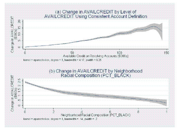 Figure 1 Data
Figure 2: Geographic Coordinates from the Credit Bureau and Census Block Group Internal Points in the Outer Banks, North Carolina
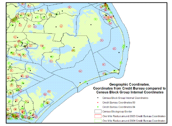 Figure 2 Description
Figure 3: Mean Credit Score by Neighborhood Racial Composition
(with 95% Confidence Interval)
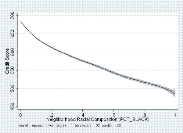 Figure 3 Data
Figure 4: Estimated Race Penalty for AVAILCREDIT and LIMIT
(with 95 Percent Confidence Interval)
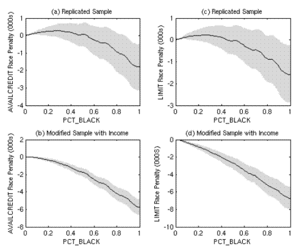 Figure 4 Data
Footnotes
The modified sample also cleans the geographic data in additional ways. The longitude and latitude coordinates supplied by the credit bureau for 2004 contained a systematic error. This error results in over 95 percent of the individuals that appear in the data twice (in 2003 and 2004) having geographic coordinates that correspond to different locations in the two time periods. By correcting for the systematic error, implied geographic mobility is substantially reduced. Return to Text