Skip to: [Printable Version (PDF)] [Bibliography] [Footnotes]

Finance and Economics Discussion Series: 2009-44 Screen Reader version ^♣

Assessing the Systemic Risk of a Heterogeneous Portfolio of Banks During the Recent Financial Crisis¹

Xin Huang ²

Hao Zhou ³

Haibin Zhu ⁴

October 2009

Abstract: This paper extends the approach of measuring and stress-testing the systemic risk of a banking sector in Huang, Zhou, and Zhu (2009) to identifying various sources of financial instability and to allocating systemic risk to individual financial institutions. The systemic risk measure, defined as the insurance cost to protect against distressed losses in a banking system, is a risk-neutral concept of capital based on publicly available information that can be appropriately aggregated across different subsets. An application of our methodology to a portfolio of twenty-two major banks in Asia and the Pacific illustrates the dynamics of the spillover effects of the global financial crisis to the region. The increase in the perceived systemic risk, particularly after the failure of Lehman Brothers, was mainly driven by the heightened risk aversion and the squeezed liquidity. The analysis on the marginal contribution of individual banks to the systemic risk suggests that "too-big-to-fail" is a valid concern from a macroprudential perspective of bank regulation.

Keywords: Systemic risk, macroprudential regulation, portfolio distress loss, credit default swap, dynamic conditional correlation.

1 Introduction

The recent global credit and liquidity crisis has led bank supervisors and regulators to rethink about the rationale of banking regulation. One important lesson is that, the traditional approach to assuring the soundness of individual banks needs to be supplemented by a system-wide macro-prudential approach. The macro-prudential perspective of supervision focuses on the soundness of the banking system as a whole and the inter-linkages between financial stability and the real economy. It has become an overwhelming theme in the policy recommendations by international policy institutions, regulators and academic researchers.⁵

Such a "systemic" view should not only cover a national banking system, but also at regional or international levels because the global banking sector has become increasingly integrated. As the current crisis has shown, vulnerabilities in one market can be easily spread abroad through various channels (e.g., loss of confidence, higher risk aversion, similarities in business models and market structures), causing disruption in market functioning and banking distresses elsewhere in the world. In Asia and the Pacific, the financial and economic integration in the past decades implies that the economic performance and the health of the banking system across countries have become more inter-related in the region.

Banks have been the most important financial intermediaries in Asia and the Pacific, by providing liquidity transformation and monitoring services, among all financial firms and the capital market channels. Historical evidence suggests that the soundness of the banking system is crucial for financial sector stability and economic growth in this region. For instance, a weak banking system was one of the key driving factors behind the 1997 Asian financial crisis. In contrast, during the current global economic and financial turmoil, the resilience of the banking sector has by far been a major support to the functioning of financial markets and an early recovery in economic growth in the region (see Bank for International Settlements (2009)).

Against such a background, this paper attempts to develop a framework to analyze the systemic risk of a portfolio of heterogeneous banks. Such analysis is based on the existing work by Huang, Zhou, and Zhu (2009), who construct a systemic risk indicator from publicly available information.⁶ In particular, they construct a systemic risk indicator with the economic interpretation as the insurance premium to cover distressed losses in a banking system, based on credit default swap (CDS) spreads of individual banks and the co-movements in banks' equity returns. Based on this methodology, this paper makes three important additional contributions.

First, we propose estimating the asset return correlation using a coherent model of dynamic conditional correlation (DCC) (Engle, 2002), such that the heterogeneous inter-connectedness of the banks in different subgroups can be well represented in the conditional correlation matrix. The original approach in Huang, Zhou, and Zhu (2009) assumes homogeneity, i.e., the pairwise correlation for any two banks is the same at a particular point in time. Such simplification is reasonable for a homogeneous system of large US banks as examined by Huang, Zhou, and Zhu (2009); but can be problematic for a portfolio of heterogeneous banks, for example, from different lines of business or from different sovereign jurisdictions.⁷

Second, the risk-neutral concept of insurance premium for distressed credit loss can be easily decomposed into various sources that are associated with changes in underlying default risks and risk premia. This can be achieved by substituting the risk-neutral default probability inferred from CDS spreads with the objective default probability estimated for each bank, like the expected default frequency (EDF) from Moody's KMV. The concept of market-based systemic risk assessment is an extension of the original idea by Merton and Perold (1993) that the capital of financial institutions is a risk-neutral concept reflected in current asset prices.⁸

Third, our study examines not only the aggregate level but also the different components of systemic risk as well. In particular, expected shortfall, the coherent concept of distressed portfolio loss, allows us to compute the marginal contribution of each bank, or each group of banks, to the systemic risk of the whole banking system. The marginal contribution of each subgroup (or each institution) adds up to the aggregate systemic risk. This additivity property is desirable from an operational perspective, because it allows the macro-prudential tools to be implemented at individual bank levels. Based on such an analysis, supervisors are able to identify systemically important financial institutions and to allocate macro-prudential capital requirements on individual banks.⁹By contrast, the standard value-at-risk (VaR) measure cannot be consistently aggregated cross subgroups, due to the lack of subadditivity (Embrechts, Lambrigger, and Wüthrich, 2009).

We apply the extended approach of Huang, Zhou, and Zhu (2009) to a portfolio of twenty-two major banks in Asia and the Pacific, spanning the period from January 2005 to May 2009. The main findings are as follows.

First, the movement in the systemic risk indicator reflects primarily the dynamics of the spillover effects of the global financial crisis to the region. Before the failure of Lehman Brothers, Australian banks were most affected and market concerns on the systemic risk of banks from other economies in the region were quite contained. This situation changed since late September 2008. Banks across the region felt the stress not only due to spillover in the financial market, but also because the performance of the real economy in the region had weakened substantially. The situation was not improved until entering the second quarter of 2009.

Second, the evolvement of market perception on the systemic risk of Asia-Pacific banks was mainly driven by the risk premium component. By contrast, concerns on increasing actual default losses explained only a small portion of the distress insurance premium, and was not able to account for the increase in the systemic risk indicator before the fourth quarter of 2008. This suggests that the stress faced by Asia-Pacific banks was mostly driven by the heightened risk aversion and liquidity squeeze in the global financial markets that are originated from the US subprime crisis.

Third, the analysis on the marginal contribution of each bank, or each bank group, to the systemic risk suggests that the size effect is very important in determining the systemic importance of individual banks. The change in the systemic risk can be largely attributed to the deterioration in credit quality (increases in default probability and/or correlation) of some largest banks. The result supports the "too-big-to-fail" concern from a macro-prudential perspective.

The remainder of the paper is organized as follows. Section 2 outlines the methodology. Section 3 introduces the data, and Section 4 presents empirical results based on an illustrative banking system that consists of twenty-two major banks in Asia and the Pacific. The last section concludes.

2 Methodology

For the purpose of macroprudential regulation of a banking system, the methodology proposed here aims to address two important issues. First, how to design a systemic risk indicator for a portfolio of heterogeneous banks? Second, how to assess the different sources of the systemic risk, i.e. to assess the contribution of each bank or each group of banks to the systemic risk indicator.

2.1 Constructing the systemic risk indicator

To address the first question of constructing a systemic risk indicator of a heterogeneous banking portfolio, we follow the recent methodology in Huang, Zhou, and Zhu (2009). The systemic risk indicator, a hypothetical insurance premium against catastrophic losses in a banking system, is constructed from real-time financial market data using the portfolio credit risk technique. The two key default risk factors, the probability of default (PD) of individual banks and the asset return correlations among banks, are estimated from credit default swap (CDS) spreads and equity price co-movements, respectively.

The one-year risk-neutral PDs of individual banks are derived from CDS spreads, using the simplified linear relationship as used in Duffie (1999), Tarashev and Zhu (2008a), and Huang, Zhou, and Zhu (2009):

$\displaystyle PD_{i,t} = \frac{a_t s_{i,t}}{a_t LGD_{i,t}+b_t s_{i,t}}$

(1)

where $a_{t}\equiv \int_t^{t+T} e^{-r \tau} d\tau$ and $b_{t}\equiv \int_t^{t+T} \tau e^{-r \tau} d\tau$ ,

is the loss-given-default and

is the risk-free rate.

It is important to point out that the PD implied from the CDS spread is a risk-neutral measure, i.e., it reflects not only the actual (or physical) default probability but also a risk premium component as well. The risk premium component can be the default risk premium that compensates for uncertain cash flow, or a liquidity premium that tends to escalate during a crisis period.

One extension in this study is that we allow for the LGD to vary, rather than assuming it to be a constant,¹⁰ over time. For example, Altman and Kishore (1996) showed that LGD can vary over the credit cycle. To reflect the comovement in PD and LGD parameters, we choose to use expected LGDs as reported by market participants who price and trade the CDS contracts.

The asset return correlation is proxied by the equity return correlation, following Huang, Zhou, and Zhu (2009). An important constraint in their approach is that the estimation of equity return correlations needs intra-day equity return data of all banks, which are not readily available for Asian countries. Therefore, we propose an alternative methodology which is applicable for banks for which only daily equity returns are available. In particular, we will apply Engle (2002)'s dynamic conditional correlation (DCC) model to estimate the time-varying equity return correlations.¹¹ The DCC method is superior to historical measures in that the correlation output refers to conditional rather than backward-looking correlation measures.

The other advantage of using the DCC method is that it allows the correlation matrix to be heterogeneous, i.e., the pairwise correlation coefficients can be different for each pair of banks.¹² The heterogeneity in correlations can have important implications on the quantitative results, as dispersion in correlation can affect the tail distribution of portfolio losses (see Hull and White, 2004; Tarashev and Zhu, 2008a, for example). This impact could be particularly important for a heterogeneous banking system for which the heterogeneity in correlations might be more remarkable, as the one we will investigate bellow.

Based on the inputs of the key credit risk parameters - PDs, LGDs, correlations, and liability weights - the systemic risk indicator can be calculated based on the simulation approach as described in Huang, Zhou, and Zhu (2009). In short, to compute the indicator, we first construct a hypothetical debt portfolio that consists of liabilities (deposits, debts and others) of all banks, weighted by the liability size of each bank. The indicator of systemic risk is defined as the insurance premium that protects against distressed losses of this portfolio. Technically, it is calculated as the risk-neutral expectation of portfolio credit losses that equal or exceed a minimum share of the sector's total liabilities.

Notice that, the definition of this "distress insurance premium" is very close to the concept of expected shortfall (ES) used in the literature, in that both refer to the conditional expectations of portfolio credit losses under extreme conditions. They differ slightly in the sense that the extreme condition is defined by the percentile distribution in expected shortfall but by a given threshold loss in distress insurance premium. Also the probabilities in the tail event underpinning ES are normalized to sum up to 1. These probabilities are not normalized for the distress insurance premium. The value-at-risk (VaR) measure is also based on the percentile distribution, but as shown by Inui and Kijima (2005) and Yamai and Yoshiba (2005), ES is a coherent measure of risk and while VaR is not.¹³

2.2 Analyzing sources of systemic risk

For the purpose of macroprudential regulation, it is important not only to monitor the level of systemic risk, but also to understand the sources of risks in a financial system. We propose to implement such a analysis from two different angles.

One perspective is to investigate how much of the systemic risk is driven by the movement in actual default risk and how much is driven by the movement in risk premia, including the default risk premium (which compensate for the uncertainty in payoff) and the liquidity risk premium (or other non-default component of the credit spread). For this purpose, we re-calculate the systemic risk indicator, but using market estimates of objective (or actual) default rates rather than the risk-neutral default rates derived from CDS spreads. The corresponding insurance premium against distress losses, on an actuarial basis, quantifies the contribution from the expected actual defaults, and the difference between the market value (the benchmark result) and the actuarial premium quantifies the contribution from risk premia components.

A second perspective is to decompose the credit risk of the portfolio into the sources of risk contributors associated with individual sub-portfolios (either a bank or a group of banks). Following Kurth and Tasche (2003) and Glasserman (2005), for standard measures of risk, including VaR, expected shortfall and the systemic indicator used in this study, the total risk can be usefully decomposed into a sum of marginal risk contributions. Each marginal risk contribution is the conditional expected loss from that sub-portfolio, conditional on a large loss for the full portfolio. In particular, if we define as the loss variable for the whole portfolio, and as the loss variable for a sub-portfolio, the marginal contribution to the systemic risk can be characterized by

$\displaystyle X$	$\displaystyle =$	$\displaystyle L+\epsilon L_i$
$\displaystyle \left. \frac{\partial X}{\partial \epsilon} \right \vert _{\epsilon \rightarrow 0}$	$\displaystyle =$	$\displaystyle E[L_i\vert L \ge L_{min}]$	(2)

Equation (2) offers a convenient working definition to calculate the marginal contribution of each sub-portfolio to the systemic risk of the whole banking portfolio. In particular, the marginal contribution of an individual bank equals the expected loss arising from this bank's default conditional on the occurrence of distressed scenarios. The technical difficulty, however, is that systemic distresses are rare events and thus ordinary Monte Carlo estimation is impractical for the calculation purpose. Therefore, we rely on the importance sampling method developed by Glassmerman and Li (2005) to simulate portfolio credit losses to improve the efficiency and precision. For the twenty-two bank portfolio in our sample, we use the mean-shifting method and generate 200,000 importance-sampling simulations of default scenarios (default or not),¹⁴ and for each scenario generate 100 simulations of LGDs.¹⁵ Based on these simulation results we calculate the expected loss of each sub-portfolio conditional on total loss exceeding a given threshold.

The approach we use to define the marginal contribution to systemic risk are closely related to two recent studies. One is the "Shapley value" decomposition approach used by Tarashev, Borio, and Tsatsaronis (2009a,b) to allocating systemic risk to individual institutions. The "Shapley value" approach, constructed in game theory, defined the contribution of each bank as a weighted average of its add-on effect to each subsystem that consists of this bank. It has the same desirable additivity property and therefore can be used as a general approach to allocating systemic risk. However, the approach suffers from the curse of dimensionality problem in that, for a system of N banks, there are possible subsystem for which the systemic risk indicator needs to be calculated.¹⁶

The other closely related approach is the CoVaR method proposed by Adrian and Brunnermeier (2008). CoVaR looks at the VaR of one portfolio (in Adrian and Brunnermeier (2008)'s case, the whole portfolio or a sub-portfolio) conditional on the VaR of another portfolio (in Adrian and Brunnermeier (2008)'s case, another sub-portfolio). In other words, the focus of CoVaR is to examine the spillover effect from one bank's failure to the safety of another bank or the whole banking system. By comparison, our working definition is along the same line but focuses on the loss of a particular bank (or a bank group) conditional on the system being in distress. It can be considered as a special case of CoES (conditional expected shortfall).¹⁷ Nevertheless, a major disadvantage of CoVaR is that it can only be used to identify systemically important institutions but cannot appropriately aggregate the systemic risk contributions of individual institutions, due to lack of subadditivity. Also CoES and CoVaR provide individual measures of systemic importance that do not sum up to the total measure of risk.

3 Data

Table 1 reports the list of banks included in this study and the summary statistics of balance sheet size, CDS spreads, and EDFs (expected default frequencies) of individual banks.

The selection of sample banks are based on their size and data availability. In the first step, we select banks from ten economies in Asia-Pacific, namely Australia, Hong Kong SAR, India, Indonesia, Korea, Malaysia, New Zealand, the Philippines, Singapore and Thailand.¹⁸ The selected banks either hold tier-1 bank capital above 2.5 billion USD or are the largest bank in its own jurisdiction. In the second step, twenty-two banks are chosen based on the data availability criteria: (i) a minimum number of 200 valid observations of daily CDS spreads since January 1, 2005; (ii) with publicly available equity prices since January 1, 2003; and (iii) a minimum number of 20 valid observations of monthly EDFs since January 2005.

The final set of twenty-two banks in our sample consists of six banks from Australia, two from Hong Kong, two from India, one from Indonesia, four from Korea, two from Malaysia, three from Singapore and two from Thailand.¹⁹ Although some large banks (e.g., HSBC Hong Kong) are missing due to data availability, the list represents a very large part of the banking system in the eight economies. At the end of 2007, the twenty-two banks combined held a total of 3.95 trillion USD assets, compared to the aggregate GDP of 4.2 trillion USD in these economies.

Our sample data cover the period from January 2005 to May 2009 and are calculated in weekly frequency. We retrieve weekly CDS spreads (together with the recovery rates used by market participants who contribute quotes of CDS spreads) from Markit,²⁰ compute dynamic conditional correlations from equity price data (which start from January 2003) provided by Bloomberg, and retrieve monthly EDFs of individual banks provided by Moody's KMV. EDF is a popular market product of estimating expected one-year (physical) default rates of individual firms based on their balance sheet information and equity price data. The method is based on the Merton (1974) framework and explained in detail in Crosbie and Bohn (2002).

Figure (1) plots the time variation in key credit risk variables: PDs, recovery rates, and correlations.

The risk-neutral PDs (top-left panel) are derived from CDS spreads using recovery rates as reported by market participants who contribute quotes on CDS spreads. The weighted averages (weighted by the size of bank liabilities) are not much different from median CDS spreads in most of the sample period. They were very low (below 0.5%) before July 2007. With the developments of the global financial crisis, risk-neutral PDs of Asia-Pacific banks increased quickly and reached a local maximum of 3.8% in March 2008, when Bear Stearns was acquired by JP Morgan. The second, and the highest, peak occurred in October 2008, shortly after the failure of Lehman Brothers. The risk-neutral PD stayed at elevated levels (6-7%) for a while, before coming back to the pre-Lehman level of 3% in April-May 2009. From a cross-sectional perspective, there were substantial differences across Asia-Pacific banks in term of credit quality, as reflected in the min-max range of their CDS spreads.

Notice that recovery rates (lower-left panel) are ex ante measures, i.e., expected recovery rates when CDS contracts are priced, and hence can differ substantially from the ex post observations of a handful default events during our sample period.²¹ In addition, whereas we allow for time-varying recovery rates, they exhibit only small variation (between 36 and 40 percent) during the sample period.²²

In contrast to the risk-neutral PDs, the physical measure of PDs -- EDFs -- of Asia-Pacific banks (top-right panel) had stayed at very low levels before the fourth quarter of 2008. The increase in EDFs since then was consistent with the deterioration in macroeconomic prospects in most Asia-Pacific economies. Exports plummeted, and economic growth slowed down substantially and turned negative in Australia, Hong Kong, Korea, Singapore and Thailand.²³ These developments generated concerns about the asset quality of banks in the region and therefore EDFs went up. However, the increases in EDFs not only came much later but also were much smaller than the corresponding hikes in the CDS spreads (or risk-neutral PDs). In addition, as the economies in the region were hit by the global crisis in different degrees, the changes in EDFs also showed substantial cross-sectional differences. The high skewness of the EDF data implies that the impact of the crisis was felt the strongest for a few banks such as Bank Negara Indonesia, Macquarie Bank, Korea Exchange Bank and Industrial Bank of Korea (Table 1).

The other key credit risk factor, the asset return correlation (lower-right panel), showed small variation over time but large cross-sectional differences. Average correlations were around 30% most of the time, before jumping up above 36% in October 2008 and staying high since then. Pairwise correlations can be as low as 10% and as high as 80%. As Figure (2) top panel shows, banks from the same country typically have much higher pairwise correlations than those from different countries.

The differences in pairwise correlations raises a concern for potential bias if the correlation matrix is assumed to be homogeneous, as did in Huang, Zhou, and Zhu (2009). Indeed, a latent-factor analysis²⁴ shows that a single-factor model can at best explain about 50% of the variation in pairwise correlations. For the portfolio of heterogeneous Asia-Pacific banks, it usually takes at least three factors to account for 90% of the cross-sectional variation in pairwise correlations (Figure 2, lower panel).²⁵

Table 2 also suggests that the key credit risk factors tend to comove with each other. Not surprisingly, the two PD measures are highly correlated, suggesting that the underlying credit quality of a bank has an important impact on the credit protection cost. PDs and correlations are also positively correlated, confirming the conventional view that when systemic risk is higher, not only the default risks of individual firms increase but they also tend to move together. Lastly, there is a significantly negative relationship between PDs and recovery rates. This is consistent with the findings in Altman and Kishore (1996) that recovery rates tend to be lower when credit condition deteriorates (procyclical).

4 Empirical findings

We apply the methodology described in Section 2 and examine the systemic risk in the heterogeneous banking system that consists of twenty-two banks from eight economies in Asia and the Pacific. It seems that, for Asia-Pacific banks, the elevated systemic risk is initially driven by rising risk premia due to a spillover effect from the global financial crisis. But since the fourth quarter of 2008 both actual default risk and risk premia (or risk aversion) have risen substantially as the global financial crisis turned into a real economic recession. Also, the more heterogeneous nature of the banks portfolio in the region, as compared to the large US banks, seems to contribute to lower systemic risk, other things equal. The marginal contribution of each individual bank to the systemic risk is mostly determined by its size, or "too big to fail", but the contagion effect of individual bank's failure to the whole banking system is more affected by correlations than sizes.

4.1 The magnitude and determinants of the systemic risk

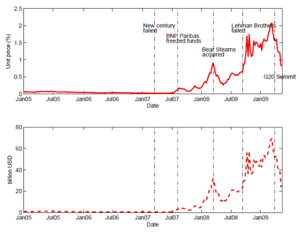
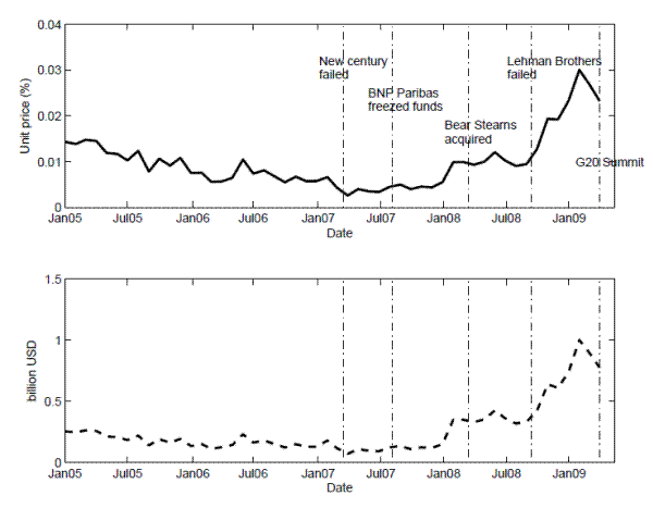
Figure 3 reports the time variation of the "distress insurance premium", in which financial distress is defined as the situation in which at least 10% of total liabilities in the banking system go into default. The insurance cost is represented as the premium rate in the upper panel and in dollar amount in the lower panel.

The systemic risk indicator for Asia-Pacific banks was very low at the beginning of the global crisis. For a long period before BNP Paribas froze three funds due to the subprime problem on August 9, 2007, the distress insurance premium for the list of twenty-two Asia-Pacific banks was merely several basis points (or less than 1 billion USD). The indicator then moved up significantly, reaching the first peak when Bear Stearns was acquired by JP Morgan on March 16, 2008.²⁶ The situation then improved significantly in April-May 2008 owing to strong intervention by major central banks.²⁷Things changed dramatically in September 2008 with the failure of Lehman Brothers. Market panic and increasing risk aversion pushed up the price of insurance against distress in the banking sector, and Asia-Pacific banks were not spared. The crisis also hit the real sector: exports fell dramatically in the region, unemployment went up, and forecasts of economic growth were substantially revised downward. The distress insurance premium hiked up and hovered in the range of 150 and 200 basis points (or 50-70 billion USD). The situation didn't improve until late March 2009. In particular, the adoption of unconventional policies and strengthened cross-border coordination among policy institutions have been effective in calming the market. Since the G20 Summit in early April 2009, the distress insurance premium has come down quickly and returned to pre-Lehman levels in May 2009, the end of our sample period.

Table 3 examines the determinants of the systemic risk indicator. The level of risk-neutral PDs is a dominant factor in determining the systemic risk, explaining alone 98% of the variation in the distress insurance premium. On average, a one-percentage-point increase in average PD raises the distress insurance premium by 28 basis points. The level of correlation also matters, but to a lesser degree and its impact is largely washed out once PD is included. This is perhaps due to the strong relationship between PD and correlation for the sample banking group during this special time period. In addition, the recovery rate has the expected negative sign in the regression, as higher recovery rates reduce the ultimate losses for a given default scenario.

Interestingly, the heterogeneity in PD and correlation inputs have an additional role in explaining the movement in the systemic risk indicator. Both the dispersion in PDs across the twenty-two banks and the dispersion in correlation coefficients²⁸ have a significantly negative effect on the systemic risk indicator. This partly supports our view that incorporating heterogeneity in PDs and correlations is important in measuring the system risk indicator.

The significantly negative effects of the dispersion factors is interesting. Theory does not predict a clear sign of these effects. Further exploration suggests that it is due to the fact that cross-section PDs and correlations are significantly negatively correlated in the given sample. At each point at time, we calculate the correlation between individual PDs and bank-specific correlations (defined in footnote 24). The correlations average -0.62 and lie in the range of [-0.78, -0.09]. This means that the banks with high correlations are the ones that have the lowest individual PDs. In other words, the banks that are likely to generate multiple defaults are less likely to default. Therefore, greater dispersion of correlations (and PDs) tends to lower the probability of default clustering and by extension reduce the cost of protection against distressed losses.

Based on the regression result (Regression 5 in Table 3), Figure 4 quantifies three sources that drive the changes in the systemic risk indicator since July 2007: changes in average PDs, changes in average correlations, and changes in heterogeneity in the banking system (as reflected in dispersion in PDs and correlations). Movements in average PDs were obviously the dominant factor in determining the systemic risk; changes in correlations and heterogeneity in the banking system, although in general of secondary importance, can have important implications particularly during the period of market turbulence. For instance, the dispersion effect reduces the systemic risk by about one third in the fourth quarter of 2008.

The results have two important implications for supervisors. First, given the predominant role of average PDs in determining the systemic risk, a first-order approximation of the systemic risk indicator could use the weighted average of PDs (or CDS spreads). This can be confirmed by comparing the similar trend in average PDs (the upper-left panel in Figure 1) and the distress insurance premium (Figure 3). Second, the average PD itself is only a good approximation but is not sufficient in reflecting the changes in the systemic risk. Correlations and heterogeneity in PDs and correlations also matter. This can be seen by comparing the two dates: October 25, 2008 and March 9, 2009. Average correlations (36.6% vs. 34.1%) and LGDs (63.2% vs. 63.6%) were similar on both dates. And the first date observed a higher average PD (7.06% vs. 6.93%) but a lower distress insurance premium (1.74% vs. 2.04%). This is mainly due to the higer dispersion in PDs (4.91% vs. 3.22%) and correlations (13.3% vs. 12.1%) on the first day, which caused the higher tail risk as explained above. In other words, diversification can reduce the systemic risk.

4.2 The role of risk premium

As mentioned in Section 2, the PDs implied from CDS spreads are a risk-neutral measure and include information not only on expected actual default losses of the banking system but also on default risk premium and liquidity risk premium components. It has been argued that, during the crisis period, the risk premium component could be the dominant factor in determining the CDS spreads (see Kim et al. (2009)). Given that the systemic risk indicator is based on risk-neutral measures, an interesting question is how much of its movement is attributable to the change in the "pure" credit quality (or actual potential default loss) of the banks and how much are driven by market sentiments (change in risk attitude, market panic, etc.) or liquidity shortage.

For the Asia-Pacific banks in this study, the first evidence is by comparing the risk-neutral PDs implied from CDS spreads with the physical (or actual) PDs estimated by Moody's KMV - EDF, the estimates of the PDs perceived by the market, as shown in the upper panels in Figure 1. In addition, Figure 5 shows the discrepancies between the two PD measures for banks from each economy (or a group of economies that consists of Indonesia, Malaysia and Thailand). As can be clearly seen, the significant increase in risk-neutral PDs between early 2008 and October 2008 was primarily driven by the heightened risk premium component. However, since October 2008, both PD measures increased sharply, reflecting the fact that global financial crisis has turned into a global economic crisis. While the loss of confidence remained as the main concern in the financial market, the spillover to the real sector led to the drop in global demand and caused significant downward revisions in forecasts of macroeconomic performance in the region. The deterioration in the real economy imposed heavy pressure on the banking system. As a result, market expectations on the health of Asia-Pacific banks were further revised down. Based on EDF data, the failure probability increased most remarkably for Korean banks.

If we use the physical PD measure (EDF) as the input, we can calculate an alternative systemic risk indicator which assumes that all risk premium components are zeros. In other words, the new indicator reflects an insurance premium on an actuarial basis, without compensation for bearing the uncertainty in payoff. Figure 6 plots the results. The level and trend of the new indicator is in sharp contrast with the benchmark result in Figure 3. First, the EDF-based indicator is much lower, which provides strong evidence on the resilience of Asia-Pacific banks during the crisis. In the worst time (early 2009), the EDF-based indicator was merely 3 basis points (or 1 billion USD), which was only a small-fraction of the CDS-based indicator. This suggests that, during a crisis period, the bailout cost of a market-based solution tends to be much larger than that justified by an objective assessment of the default losses, because of risk aversion and liquidity dry-up. Second, CDS spreads (main drivers of risk premium) typically lead bank equity prices (main drivers of EDFs) at the early stages of the crisis. The EDF-based indicator shows that actual credit problem did not deteriorate before the fourth quarter of 2008; even after then the credit quality deterioration for Asia-Pacific banks has remained contained. This provides a very different picture from the benchmark case with risk-neutral PD measure.²⁹

In addition, we also run a regression analysis that examines the impact of actual default rates and risk premium factors on the systemic risk indicator. In Table 4, objective default risk (or actual default rates) is measured by average EDFs of sample banks, the default risk premium in the global market is proxied by the difference between Baa- and Aaa-rated corporate bond spreads in the US market (see Chen, Collin-Dufresne, and Goldstein (2008)), and the liquidity risk premium in the global market is proxied by the LIBOR-OIS spread in the US market (see Brunnermeier (2009)). Individually (regressions 1 to 3), each of the three factors has a significant impact on the systemic risk indicator with expected sign. The last regression includes all three factors, which remain statistically significant. Figure 7 quantifies the contribution of actual default risk, default risk premium and liquidity risk premium in explaining the changes in systemic risk since July 2007. On average, the default risk premium component explains about 40% of the movement in the systemic risk; actual default risk comes next, explaining about 30%;³⁰ liquidity risk premium is also important, explaining 15-20% of changes in the systemic risk indicator. The decomposition results provide strong evidence that contagion in the banking sector in Asia and the Pacific stemmed not only from a reassessment of default risks but also more importantly from a global repricing of risk and the dry-up in liquidity.

4.3 Sources of vulnerabilities

The other natural question is the sources of vulnerabilities, i.e. which banks are systemically more important or contribute the most to the increased vulnerability? Using the methodology described in Section 2, we are able to provide an answer to this question based on simulation results shown in Figure 8.

In Figure 8, banks are divided into six groups: Australian banks, Hong Kong banks, Indian banks, Korean banks, Singapore banks and banks from Indonesia, Malaysia and Thailand. We calculate the marginal contributions of each group of banks to the systemic risk indicator, both in level terms and in percentage terms. In relative term, the marginal contribution of each group of banks were quite stable before mid-2008. Australian banks were obviously the most important ones and contributed the most to the systemic vulnerability. However, since September 2008, the relative contribution of Australian banks decreased substantially, whereas banks from Hong Kong and Singapore became more important from a systemic perspective.

Table 5 provides further details on the marginal contribution of each bank at five dates: (i) June 30, 2007: the inception of the global financial crisis; (ii) March 15, 2008: the first peak of the crisis when Bear Stearns was acquired by JP Morgan; (iii) October 25, 2008: the second peak of the crisis, shortly after the failure of Lehman Brothers; (iv) March 7, 2009: when the systemic risk indicator reached the highest level observed during our sample period; and (v) May 2, 2009: one month after the G20 London Summit and towards the end of our sample period.

Several observations are worthy of special remark. First, the biggest contributors to the systemic risk, or the systemically important banks, often coincide with the biggest banks in the region. One example is National Australia Bank, the biggest bank in our sample set. Although its CDS spread (or implied PD) is relatively low compared to the other banks, its contribution to the systemic risk has always been one of the highest. By contrast, some banks with very high CDS spreads, but smaller in size (e.g. Woori Bank and Korean Exchange Bank), are considered not to be systemically important for the region based on marginal contribution analysis. Second, one can compare the systemic risk contribution of each bank with its equity capital position to judge the source of vulnerability of the banking system. It is clear that, at the beginning phase of the crisis, Australian banks were most affected in that they explained the majority of the increase in the systemic risk, and the risk contribution is 20-30% of their equity capital position. Since the failure of Lehman Brothers, other Asian banks were almost all severely hit. For instance, the systemic risk contribution of Standard Chartered Bank (Hong Kong) was as high as 14 billion USD on March 7, 2009, approximately two thirds of its equity capital. Were the risk materialized, this category of banks are most likely to face difficulty in raising fresh equity from the market and therefore warrant special attention from systemic risk monitors or regulators.

Table 6 examines the determinants of marginal contribution to the systemic risk for each bank, using an OLS regression on the panel data. To control for bias, we use clustered standard errors grouped by banks as suggested by Peterson (2009). The first regression shows that weight, or the size effect, is the primary factor in determining marginal contributions both in level and in relative terms. This is not surprising, given the conventional "too-big-to-fail" concern and the fact that bigger banks often have stronger inter-linkage with the rest of the banking system. Default probabilities also matter, but to a lesser extent and its significance disappears in the relative-term regression. This supports the view for distinguishing between micro- and macro-prudential perspectives of banking regulation, i.e., the failure of individual banks does not necessarily contribute to the increase in systemic risk. The second and third regressions suggest that there are significant interactive effects. Adding interactive terms between weight and PD or correlation have additional and significant explanatory power. Overall, the results suggest that the marginal contribution is the highest for high-weight (i.e. large) banks which observe increases in PDs or correlations.

As discussed earlier, our marginal contribution measure is an alternative measure related to the CoVaR measure suggested by Adrian and Brunnermeier (2008), i.e., the conditional expected loss associated with bank if total losses exceed a threshold. Using the same simulation toolbox, we are also able to calculate the conditional expected losses of the whole banking system if bank defaults. The results are shown in Table 7, in which the first measure refers to conditional expected losses of the whole banking system and the second measure refers to conditional expected losses of all other banks, i.e., excluding bank itself.

This conditional expected system loss measure, in addition to our marginal loss contribution measure, provides some complimentary information on the systemic linkages among banks. Instead of showing the resilience of a particular bank during a banking distress (as indicated in the marginal contribution measure), this measure shows the contagion effect due to individual bank's failure. Some small banks, which are not too big to fail, can have important spillover effects because they are well connected or similar to other banks in the system. To cite two examples, St George Bank, a medium-size Australian bank in the sample, is not a major contributor to the systemic risk but its failure is very likely to be associated with a deterioration of the banking system. This is due to its highly correlated fragility with other Australian banks. On the other hand, Standard Chartered Bank (Hong Kong) is a major contributor to the systemic risk, but the contagion effect due to its failure is quite contained due to its low correlation with other banks.

5 Concluding remarks

The current global financial crisis has caused policymakers to reconsider the institutional framework for overseeing the stability of their financial systems. At an international level, a series of recommendations have been made covering various aspects of financial regulation and supervision. It has become generally accepted that the traditional microprudential or firm-level approach to financial stability needs to be complemented with a system-wide macroprudential approach, i.e., to pay greater attention to individual institutions that are systemically important.

In this paper we extend the methodology in Huang, Zhou, and Zhu (2009) to examine the systemic risk in a heterogeneous banking system that consists of twenty-two banks from eight economies in Asia and the Pacific. Our results are helpful to understand the spillover mechanism of the international crisis to the region. It seems that the elevated systemic risk in the region is initially driven by the rising risk aversion, as a spillover effect from the global financial crisis. But since the fourth quarter of 2008, both actual default risk and risk premia are rising as the global financial crisis turned into a real economic recession. A decomposition analysis shows that the marginal contribution of individual banks to the systemic risk is mostly determined by its size, or the "too big to fail" doctrine.

Our approach makes a first attempt toward the changing direction in bank supervision and regulation, among many concurrent studies. The methodology proposed in this paper provides a possible operational tool to solve important questions in this area: How to measure the systemic risk of a financial system? How to identify systemically important financial institutions? How to allocate systemic capital charge to individual banks? Going forward, a fruitful area for future research is to develop and improve an operational framework, including the appropriate policy instruments, to conduct macroprudential supervision and to assess a systemic capital charge. Challenges remain on both the methodology and implementation fronts.

Bibliography

Adrian, Tobias and Markus Brunnermeier (2008),

"CoVaR," Federal Reserve Bank of New York Staff Reports.

Aït-Sahalia, Yacine and Andrew Lo (2000),

"Nonparametric risk management and implied risk aversion," Journal of Econometrics, vol. 94, 9-51.

Altman, Edward and Vellore Kishore (1996),

"Almost everything you want to know about recoveries on default bonds," Financial Analysts Journal, vol. 52, 57-64.

Avesani, Renzo, Antonio Garcia Pascual, and Jing Li (2006),

"A new risk indicator and stress testing tool: A multifactor nth-to-default CDS basket," IMF Working Paper.

Bank for International Settlements (2009),

"The international financial crisis: timeline, impact and policy response in Asia and the Pacific," Presented at the Wrap-up conference of the BIS Asian Research Programme.

Borio, Claudio (2003),

"Towards a macro-prudential framework for financial supervision and regulation?" BIS Working Papers.

Brunnermeier, Markus, Andrew Crockett, Charles Goodhart, Avinash Persaud, and Hyun Shin (2009),

"The fundamental principles of financial regualtions," Geneva Reports on the World Economy.

Brunnermeier, Markus K. (2009),

"Deciphering the 2007-08 Liquidity and Credit Crunch," Journal of Economic Perspectives, vol. 23, 77–-100.

Chen, Long, Pierre Collin-Dufresne, and Robert S. Goldstein (2008),

"On the Relation between Credit Spread Puzzles and the Equity Premium Puzzle," Journal of Economic Perspectives, forthcoming.

Crocket, Andrew (2000),

"Marrying the micro- and macro-prudential dimensions of financial stbility," Speech before the Eleventh International Conference of Banking Supervisors, Basel.

Crosbie, Peter and Jeffrey Bohn (2002),

"Modeling default risk," KMV White Paper.

Duffie, Darrall (1999),

"Credit swap valuation," Financial Analysts Journal, pages 73-87.

Embrechts, Paul, Dominik D. Lambrigger, and Mario V. Wüthrich (2009),

"On extreme value theory, aggregation and diversification in finance," Working Paper, Department of Mathematics, ETH Zurich.

Engle, Robert (2002),

"Dynamic donditional dorrelation: A simple class of multivariate generalized autoregressive conditional heteroskedasticity models," Journal of Business and Economic Statistics, vol. 20, 339-350.

Financial Stability Forum (2009a),

"Reducing procyclicality arising from the bank capital framework," Joint FSF-BCBS Working Group on Bank Capital Issues.

Financial Stability Forum (2009b),

"Report of the Financial Stability Forum on addressing procyclicality in the financial system," April.

Glasserman, Paul (2005),

"Measuing marginal risk contributions in credit portfolios," Journal of Computational Finance, vol. 9, 1-41.

Glassmerman, Paul and Jingyi Li (2005),

"Importance sampling for portfolio credit risk," Management Science, vol. 51, 1643-1656.

Heaton, John, Deborah Lucas, and Robert McDonald (2008),

"Is mark-to-market accounting destablizing? Analysis and implications for policy," Working Paper, University of Chicago and Northwestern University.

Heitfield, Eric, Steve Burton, and Souphala Chomsisengphet (2006),

"Systematic and idiosyncratic risk in syndicated loan portfolios," Journal of Credit Risk, vol. 2, 3-31.

Huang, Xin, Hao Zhou, and Haibin Zhu (2009),

"A framework for assessing the systemic risk of major financial institutions," Journal of Banking and Finance, forthcoming.

Hull, John and Alan White (2004),

"Valuation of a CDO and an n-th to default CDS without Monte Carlo simulation," Journal of Derivatives, vol. 12, 8-23.

Inui, Koji and Masaaki Kijima (2005),

"On the significance of expected shortfall as a coherent risk measure," Journal of Banking and Finance, vol. 29, 853-864.

Kim, Don, Mico Loretan, and Eli Remolona (2009),

"Contagion and risk premia in the amplification of crisis: Evidence from Asian names in the CDS market," Working Paper.

Kurth, Alexandre and Dirk Tasche (2003),

"Credit risk contributions to value-at-risk and expected shortfall," Risk, vol. 16, 84-88.

Lehar, Alfred (2005),

"Measuring systemic risk: A risk management approach," Journal of Banking and Finance, vol. 29, 2577-2603.

Merton, Robert (1974),

"On the pricing of corporate debt: The risk structure of interest rates," Journal of Finance, vol. 29, 449-470.

Merton, Robert and André Perold (1993),

"Theory of risk capital in financial firms," Journal of Applied Corporate Finance, vol. 6, 16-32.

Panetta, Fabio, Paolo Angelini, Ugo Albertazzi, Francesco Columba, Wanda Cornacchia, Antonio Di Cesare, Andrea Pilati, Carmelo Salleo, and Giovanni Santini (2009),

"Financial sector pro-cyclicality: lessons from the crisis," Banca D'Italia Occasional Papers.

Peterson, Mitchell (2009),

"Estimating standard errors in finance panel data sets: Comparing approaches," Review of Financial Studies, vol. 22, 435-480.

Tarashev, Nikola, Claudio Borio, and Kostas Tsatsaronis (2009a),

"Allocating systemic risk to individual institutions: Methodology and policy applications," working paper.

Tarashev, Nikola, Claudio Borio, and Kostas Tsatsaronis (2009b),

"The systemic importance of financial institutions," BIS Quarterly Review.

Tarashev, Nikola and Haibin Zhu (2008a),

"The pricing of portfolio credit risk: Evidence from the credit derivatives market," Journal of Fixed Income, vol. 18, 5-24.

Tarashev, Nikola and Haibin Zhu (2008b),

"Specification and calibration errors in measures of portfolio credit risk: The case of the ASRF model," International Journal of Central Banking, vol. 4, 129-174.

Yamai, Yasuhiro and Toshinao Yoshiba (2005),

"Value-at-risk versus expected shortfall: A practical perspective," Journal of Banking and Finance, vol. 29, 997-1015.

Appendix

A. Estimating heterogeneous equity return correlations using the DCC model

We apply Engle (2002)'s dynamic conditional correlation (DCC) model to estimate the time-varying heterogeneous equity return correlations among the Asian banks in this paper.

Let $r_{i,t}$ be the daily return of bank on day . The conditional standard deviation is

$\displaystyle h_{i,t}=E_{t-1}(r^2_{i,t}), \quad r_{i,t}=\sqrt{h_{i,t}} \epsilon_{i,t}, \,\, i=1, 2, ..., 22.$

Let be the column vector of daily returns of all banks on day , $r_t=[r_{1,t}, r_{2,t}, ..., r_{22,t}]'$ . The conditional covariance matrix of is

$\displaystyle E_{t-1}(r_t r_t') \equiv H_t$

The DCC model is specified as follows

$\displaystyle H_t = D_t R_t D_t, \quad \mathrm{where} D_t = diag\{\sqrt{h_{i,t}}\},$

and

is the conditional correlation matrix, our estimation target.

To model the process, let's assume that the conditional covariance matrix of $\epsilon$ 's is . Its i'th row, j'th column element $q_{i,j,t}$ following the GARCH(1,1) model:

$\displaystyle q_{i,j,t} = \bar{\rho}_{i,j} + \alpha (\epsilon_{i,t-1} \epsilon_{j,t-1} - \bar{\rho}_{i,j}) + \beta(q_{i,j,t-1}-\bar{\rho}_{i,j})$

$\bar{\rho}_{i,j}$ is the unconditional correlation between $\epsilon_{i,t}$ and $\epsilon_{j,t}$ , $\bar{q}_{i,j} \cong \bar{\rho}_{i,j}$ .

The i'th row, j'th column element in the matrix is

$\displaystyle \rho_{i,j,t} = \frac{q_{i,j,t}}{\sqrt{q_{i,i,t}q_{j,j,t}}}$

So the correlation matrix

will be positive definite, as it is the correlation matrix from the covariance matrix

The matrix version of the above model is

$\displaystyle Q_t = S(1-\alpha-\beta) + \alpha(\epsilon_{t-1}\epsilon_{t-1}') + \beta Q_{t-1},$

where

is the unconditional covariance matrix of $\epsilon$ 's.

To estimate the DCC model, we make the following statistical specification:

		$\displaystyle r_t\vert I_{t-1} \sim N(0, D_t R_t D_t),$
		$\displaystyle D^2_t = diag\{\omega_i\} + diag\{\kappa_i\} \circ r_{t-1} r'_{t-1} + diag \{\lambda_i\} \circ D^2_{t-1},$
		$\displaystyle \epsilon_t = D^{-1}_t r_t,$
		$\displaystyle Q_t = S (1 - \alpha - \beta) + \alpha \epsilon_{t-1} \epsilon'_{t-1} + \beta Q_{t-1},$
		$\displaystyle R_t = diag \{Q_t\}^{-1} Q_t diag \{Q_t\}^{-1}.$

where $\circ$ is the Hadamard element-by-element product of two matrices with the same size. We estimate the DCC model by quasi-maximum likelihood estimation method, to be robust to possible mis-specification of the normal distribution. Then we extract the latent time-varying conditional correlation matrix

from the data using the DCC model and the parameter estimates.

Table 1: List of twenty-two banks in Asia-Pacific

	Country	Equity¹	Liability¹	CDS spreads²: Period 1	CDS spreads²: Period 2	CDS spreads²: Period 3	EDF³: Period 1	EDF³: Period 2	EDF³: Period 3
ANZ National Bank	Australia	19.53	328.39	8.30	38.70	131.66	1.29	2.19	6.86
Commonwealth Bank Group	Australia	25.01	437.75	8.44	39.22	127.23	4.75	2.67	4.43
Macquarie Bank	Australia	9.19	143.60	15.44	94.68	491.44	5.63	10.24	196.29
National Australia Bank	Australia	26.47	482.17	8.44	39.56	133.90	5.88	4.62	11.00
St George Bank	Australia	5.21	106.22	11.62	47.69	128.08	3.38	3.76	17.33
Westspac Banking Corp	Australia	15.79	318.73	8.44	39.14	125.28	3.33	3.38	7.43
Bank Negara Indonesia	Indonesia	1.84	17.68	113.27	166.18	545.23	30.12	72.48	439.57
ICICI Bank	India	11.42	109.65	72.10	170.15	593.10	n.a.	7.75	87.14
State Bank of India	India	15.77	240.34	59.95	115.08	348.07	13.50	19.19	106.57
Bank of East Asia	Hong Kong	3.90	46.61	22.79	40.50	276.32	2.83	3.86	64.71
Standard Chartered Bank	Hong Kong	21.45	307.75	25.93	87.96	470.97	n.a.	n.a.	n.a.
Industrial Bank of Korea	Korea	7.14	120.32	25.44	66.64	385.05	20.21	10.24	138.14
Kookmin Bank	Korea	17.13	216.70	28.43	75.20	387.59	n.a.	n.a.	n.a.
Korea Exchange Bank	Korea	7.11	80.53	33.53	67.35	398.09	8.04	8.71	114.57
Woori Bank	Korea	14.05	2.27	31.10	88.86	451.84	12.92	6.67	56.29
Malayan Banking Berhad	Malaysia	6.15	76.21	23.92	48.28	218.55	4.54	4.33	25.57
Public Bank Berhad	Malaysia	3.02	49.65	26.87	52.61	220.05	2.25	2.33	7.00
DBS Bank	Singapore	16.10	146.30	8.63	32.64	130.25	6.08	2.67	10.86
Oversea Chinese Banking Corp	Singapore	11.71	109.69	9.32	32.45	128.24	1.46	1.90	11.14
United Overseas Bank Ltd	Singapore	12.32	109.31	10.60	33.16	133.10	4.96	3.24	9.86
Bangkok Bank	Thailand	5.62	48.10	40.83	68.26	317.90	4.88	5.38	24.57
Kasikornbank	Thailand	3.37	30.17	36.07	64.77	269.92	7.58	7.67	39.14

Notes:

In billions of US dollars. 2007 data.

Average daily CDS spreads in each period, in basis points. "Period 1" starts from January 1, 2005 and ends on December 31, 2006; "Period 2" starts from January 1, 2007 and ends on September 15, 2008; "Period 3" starts from September 16, 2008 and ends on May 20, 2009.

Average monthly EDFs in each period, in basis points. "Period 1" starts from January 2005 and ends in December 2006; "Period 2" starts from January 2007 and ends in September 2008; "Period 3" starts from October 2008 and ends in April 2009.
Sources: Bloomberg; Markit; Moody's KMV.

Table 2: Relationship between key credit risk factors

	CDS	PD	EDF	COR	REC
CDS	1	1.00/1.00	0.89/0.78	0.78/0.70	-0.55/-0.58
PD		1	0.88/0.78	0.77/0.70	-0.54/-0.57
EDF			1	0.73/0.61	-0.60/-0.58
COR				1	-0.42/-0.38
REC					1

Notes: The table summarizes the relationship between key credit risk factors: CDS spreads (CDS), risk-neutral PDs implied from CDS spreads (PD), EDFs, asset return correlations (COR) and recovery rates (REC). In each cell, the first number reports the bivariate correlation between two time series of cross-sectional averages, and the second number reports the average of bank-specific bivariate correlation coefficients. Bank-specific asset return correlation is defined as the average asset return correlation between one bank and all others.

Table 3: Determinants of systemic risk indicator

	Regression 1	Regression 2	Regression 3	Regression 4	Regression 5
Constant	-0.11	-5.69	11.21	0.19	1.44
Constant t-statistics	(16.8)	(18.5)	(10.7)	(0.8)	(5.1)
Average PD	27.66			25.40	29.24
Average PD t-statistics	(99.2)			(57.9)	(30.8)
Average Correlation		19.85		1.85	2.25
Average Correlation t-statistics		(19.7)		(5.1)	(6.6)
Recovery rate			-28.60	-2.17	-12.44
Recovery rate t-statistics			(10.4)	(3.9)	(6.4)
Dispersion in PD					-4.90
Dispersion in PD t-statistics					(6.4)
Dispersion in correlation					-3.77
Dispersion in correlation t-statistics					(7.3)
Adjusted-R	0.98	0.63	0.32	0.98	0.99

Notes: The dependent variable is the indicator of systemic risk for a group of major Asia-Pacific banks, defined as the unit price (in per cent) of insurance against distressed losses. Dispersion refers to the standard deviation of the variable of interest (PD or correlation) for the sample banks at each particular point in time. PD refers to risk-neutral probability of default implied from CDS spreads, and correlation of each bank refers to its average correlation coefficient with the other banks. t-statistics are in the parenthesis.

Table 4: Determinants of systemic risk indicator: further analysis

	Regression 1	Regression 2	Regression 3	Regression 4
Constant	-0.061	-0.49	0.013	-0.31
Constant t-statistics	(1.9)	(12.5)	(0.2)	(7.8)
Average EDF (%)	3.44			1.50
Average EDF (%) t-statistics	(17.6)			(5.6)
Baa-Aaa spread (%)		0.64		0.33
Baa-Aaa spread (%) t-statistics		(23.6)		(5.5)
LIBOR-OIS spread (%)			0.68	0.13
LIBOR-OTS spread (%) t-statistics			(8.6)	(2.8)
Adjusted-R	0.86	0.92	0.60	0.95

Table 5: Marginal contribution to the systemic risk by bank on specific dates

	Country	Marginal contribution by bank: 06.30.2007	Marginal contribution by bank: 03.15.2008	Marginal contribution by bank: 10.25.2008	Marginal contribution by bank: 03.07.2009	Marginal contribution by bank: 05.02.2009	Memo: Bank equity in 2007
ANZ National Bank	Australia	0.0771	4.3900	5.7229	7.7300	4.2279	19.53
Commonwealth Bank Group	Australia	0.2156	6.5001	8.2839	10.6668	5.8130	25.01
Macquarie Bank	Australia	0.0254	1.5436	3.1761	3.6251	1.9618	9.19
National Australia Bank	Australia	0.1678	7.6246	9.4217	12.8181	7.7941	26.47
St George Bank	Australia	0.0153	1.2026	1.2868	n.a.	n.a.	5.21
Westspac Banking Corp	Australia	0.0829	4.1081	5.0966	7.1203	3.8562	15.79
Bank Negara Indonesia	Indonesia	0.0010	0.0355	0.1880	0.1634	0.0736	1.84
ICICI Bank	India	0.0076	0.4466	2.2754	1.6353	0.8748	11.42
State Bank of India	India	0.0203	0.8543	4.2207	2.8282	1.6166	15.77
Bank of East Asia	Hong Kong	0.0006	0.0766	0.4563	0.4446	0.2293	3.90
Standard Chartered Bank	Hong Kong	0.0427	2.1363	8.7825	13.9914	9.8628	21.45
Industrial Bank of Korea	Korea	0.0082	0.3868	1.8831	1.4536	0.7631	7.14
Kookmin Bank	Korea	0.0227	1.0698	n.a.	n.a.	n.a.	17.13
Korea Exchange Bank	Korea	0.0031	0.2298	1.0202	0.8903	0.5462	7.11
Woori Bank	Korea	0.0000	0.0079	0.0298	0.0337	0.0176	14.05
Malayan Banking Berhad	Malaysia	0.0017	0.1153	0.6716	0.5053	0.2547	6.15
Public Bank Berhad	Malaysia	0.0009	0.0478	0.4375	0.3564	0.1675	3.02
DBS Bank	Singapore	0.0083	0.4285	1.7736	1.6141	0.9914	16.10
Oversea Chinese Banking Corp	Singapore	0.0040	0.2743	1.1038	0.9588	0.5424	11.71
United Overseas Bank Ltd	Singapore	0.0040	0.2372	1.0737	0.9895	0.5696	12.32
Bangkok Bank	Thailand	0.0013	0.0672	0.3921	0.3688	0.2682	5.62
Kasikornbank	Thailand	0.0008	0.0396	0.3130	n.a.	n.a.	3.37
*Total*		0.7113	31.8225	57.6092	68.1939	40.4308	259.32

Notes: All numbers are in billions of US dollars.

Table 6: Determinants of marginal contribution to the systemic risk
Panel 1. Level regressions

	Regression 1: Coef.	Regression 1: t-stat	Regression 2: Coef.	Regression 2: t-stat	Regression 3: Coef.	Regression 3: t-stat
Constant	-5.24	(2.2)	-0.45	(2.2)	5.28	(3.1)
PD $_{i,t}$	0.78	(2.4)			-0.51	(2.2)
Cor $_{i,t}$	9.30	(1.4)			-16.05	(3.7)
Weight $_{i,t}$	54.89	(7.8)	-160.83	(4.0)	-253.29	(4.2)
PD $_{i,t} \times$ Weight $_{i,t}$			27.88	(5.0)	36.05	(4.7)
Cor $_{i,t} \times$ Weight $_{i,t}$			485.31	(5.0)	730.86	(5.0)
Adjusted-R	0.40		0.81		0.86

Table 6: Determinants of marginal contribution to the systemic risk
Panel 2. Relative-term regressions

	Regression 1: Coef.	Regression 1: t-stat	Regression 2: Coef.	Regression 2: t-stat	Regression 3: Coef.	Regression 3: t-stat
Constant	-7.52	(2.2)	-2.07	(2.6)	9.57	(4.1)
PD $_{i,t}$	0.22	(0.5)			-0.15	(0.3)
Cor $_{i,t}$	4.05	(1.1)			-12.04	(5.4)
Weight $_{i,t}$	172.72	(5.1)	-165.09	(2.1)	-355.35	(3.7)
PD $_{i,t} \times$ Weight $_{i,t}$			15.53	(0.9)	23.45	(1.2)
Cor $_{i,t} \times$ Weight $_{i,t}$			272.35	(4.9)	450.35	(6.2)
Adjusted-R	0.83		0.89		0.92

Notes: The dependent variable is the marginal contribution of each bank to the systemic risk indicator, which is represented in level terms (unit cost of insurance, in basis point) in the first panel and in relative terms (as a percentage of total insurance premium) in the second panel. Explanatory variables include PDs, bank-specific correlations (average of pairwise correlations between one bank and all others) and weights of individual banks and interactive terms. Similarly, PDs and correlations refer to level terms in the first panel and relative terms (the ratio over cross-sectional averages) in the second panel. OLS regression is adopted and t-statistics are reported in the parenthesis, using clustered standard errors grouped by banks.

Table 7: Expected losses of the banking system conditional on the failure of bank

on specific dates

	Measure 1: 10.25.2008	Measure 1: 03.07.2009	Measure 2: 10.25.2008	Measure 2: 03.07.2009
ANZ National Bank	724.22	729.99	517.93	524.59
Commonwealth Bank Group	752.49	779.29	480.46	504.63
Macquarie Bank	426.62	369.13	337.80	280.54
National Australia Bank	751.35	768.48	450.45	464.24
St George Bank	535.88	564.62	469.59	497.36
Westspac Banking Corp	715.46	721.06	515.34	520.78
Bank Negara Indonesia	190.97	158.48	180.05	147.24
ICICI Bank	275.54	255.45	207.80	187.15
State Bank of India	319.20	314.66	171.40	165.97
Bank of East Asia	305.67	272.79	276.86	243.77
Standard Chartered Bank	397.63	398.83	208.87	208.28
Industrial Bank of Korea	334.20	322.44	259.16	247.41
Kookmin Bank	392.13	356.34	258.01	221.82
Korea Exchange Bank	296.25	278.48	246.88	229.40
Woori Bank	270.80	250.91	269.38	249.50
Malayan Banking Berhad	248.85	224.32	201.15	176.89
Public Bank Berhad	231.46	223.99	200.32	192.64
DBS Bank	444.59	447.97	355.84	356.69
Oversea Chinese Banking Corp	391.03	394.03	322.78	326.37
United Overseas Bank Ltd	372.09	398.16	304.46	330.81
Bangkok Bank	244.96	247.36	215.37	217.05
Kasikornbank	243.62	225.96	224.99	207.22

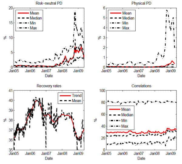
Notes: All numbers are in billions of US dollars. Measure 1 refers to expected losses of the whole banking system conditional on bank i's failure; Measure 2 is similar and refers to expected loss of the rest of the banking system (excluding bank i) conditional on bank i's failure.

**Figure 1:** Credit risk variables

Note: This graph plots the time series of key credit risk factors: risk-neutral PDs implied from CDS spreads, physical PDs (EDFs) reported by Moody's KMV, recovery rates and average correlations calculated from comovement in equity returns using the DCC method.

**Figure 2:** Correlation estimates

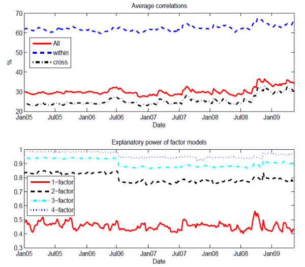
Note: The upper panel plots the averages of pairwise correlations (based on equity return movements) for three categories: for any two banks from the sample, for any two banks from the same jurisdiction area, and for any two banks from different jurisdiction areas. The lower panel shows, on each day, how much a latent-factor model can explain the cross-section variation in the correlation matrix.

**Figure 3:** Systemic Risk Indicator of Asia Banking Sector
$Figure 3: The graph plots the systemic risk indicator for the Asian banking system, defined as the price for insuring against financial distresses (at least 10\% of total liabilities in the banking system are in default). The price is shown as the cost per unit of exposure to these liabilities in the upper panel and is shown in dollar term in the lower panel.$

Note: The graph plots the systemic risk indicator for the Asian banking system, defined as the price for insuring against financial distresses (at least 10% of total liabilities in the banking system are in default). The price is shown as the cost per unit of exposure to these liabilities in the upper panel and is shown in dollar term in the lower panel.

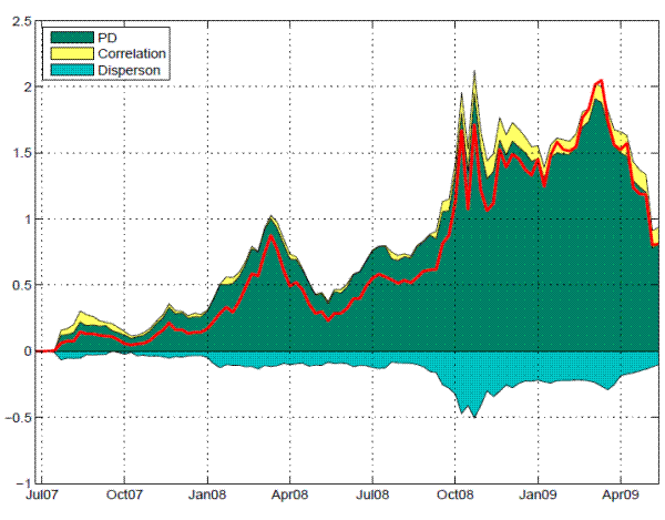
**Figure 4:** Contributing Factors to the Systemic Risk Indicator

Note: The graph plots the contribution effect of average PDs, average correlations, dispersion in PDs and correlations in determining the changes in the systemic risk indicator since July 2007. It is based on the regression results as specified in regression 5 of Table 3.

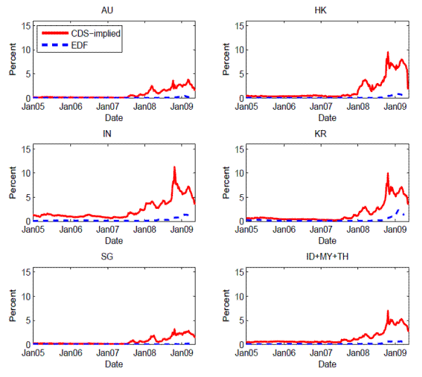
**Figure 5:** Actual vs. risk-neutral default rates by region

Note: The graph plots the risk-neutral versus physical PDs in each of the six economic areas1. The risk-neutral PDs are derived from CDS spreads and the physical PDs refer to EDFs provided by Moody's KMV.
¹ AU: Australia; HK: Hong Kong SAR; IN: India; KR: Korea; SG: Singapore; ID+MY+TH: Indonesia, Malaysia and Thailand.

**Figure 6:** Systemic Risk Indicator based on EDFs
$Figure 6: The graph plots the systemic risk indicator for the Asian banking system, based on the same definition as in Figure \ref{fig:indicator} but using physical PD measures (i.e., EDF) to replace risk-neutral PDs derived from CDS spreads. The indicator is shown in unit cost (per unit of total liability) in the upper panel and in dollar term in the lower panel.$

Note: The graph plots the systemic risk indicator for the Asian banking system, based on the same definition as in Figure 3 but using physical PD measures (i.e., EDF) to replace risk-neutral PDs derived from CDS spreads. The indicator is shown in unit cost (per unit of total liability) in the upper panel and in dollar term in the lower panel.

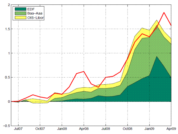
**Figure 7:** Contributing Factors to the Systemic Risk Indicator

Note: The graph plots the contribution effect of actual default risk, default risk premium, and liquidity risk premium in determining the changes in the systemic risk indicator since July 2007. It is based on the regression results as specified in regression 4 of Table 4.

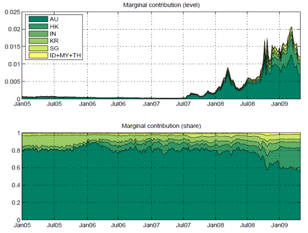
**Figure 8:** Marginal contribution to systemic risk by region

Note: The figure shows the marginal contribution of banks from each economic area1 to the systemic risk indicator, the distress insurance premium in unit cost term. The contribution is shown in level term in the upper panel and as a percentage of the total risk in the lower panel.
¹AU: Australia; HK: Hong Kong SAR; IN: India; KR: Korea; SG: Singapore; ID+MY+TH: Indonesia, Malaysia and Thailand.

Footnotes

1. We thank Clara Garcia and Jhuvesh Sobrun for excellent research assistance. The views presented here are solely those of the authors and do not necessarily represent those of the Federal Reserve Board or the Bank for International Settlements. Return to Text

2. Department of Economics, University of Oklahoma, Norman, Oklohoma, USA; phone: 1-405-325-2643; e-mail: [email protected]. Return to Text

3. Risk Analysis Section, Federal Reserve Board, Washington, D.C., USA; phone: 1-202-452-3360; e-mail: [email protected]. Return to Text

4. Bank for International Settlements, Representative Office for Asia and the Pacific, Hong Kong; phone: 852-2878-7145; e-mail: [email protected]. Return to Text

5. See, for instance, Brunnermeier, Crockett, Goodhart, Persaud, and Shin (2009), Financial Stability Forum (2009a), Financial Stability Forum (2009b) and Panetta, Angelini, Albertazzi, Columba, Cornacchia, Cesare, Pilati, Salleo, and Santini (2009), among others. The macro-prudential perspective was first proposed by Crocket (2000) and Borio (2003). Return to Text

6. Along the same line, Lehar (2005) and Avesani, Pascual, and Li (2006) proposed alternative market-based indicators of systemic risk. These indicators are useful supplementary measures to balance sheet information, such as the Financial Soundness Indicators used in the Financial Sector Assessment Program (FSAP). In addition, supervisors sometimes implement risk assessments based on confidential banking information, such as the Supervisory Capital Assessment Program (SCAP) implemented by the U.S. regulatory authorities in early 2009 and the European-wide stress testing program sanctioned by the Committee of European Banking Supervisors (CEBS). Return to Text

7. Huang, Zhou, and Zhu (2009) also rely on high-frequency tick-by-tick equity price data to construct and forecast the realized correlations, while the dynamic conditional correlation (DCC) approach adopted here only requires a daily frequency of equity prices. Return to Text

8. A recent paper by Heaton, Lucas, and McDonald (2008) explicitly argues that capital reserve is a risk-neutral measurement. Along the same line, Aït-Sahalia and Lo (2000) regard value-at-risk (VaR) as inherently a risk-adjusted quantity implied by financial markets. Notice that this is a concept of "economic capital" (Merton and Perold, 1993) reflected in the market expectation of potential losses, which differs from the concept of "regulatory capital" based on the actuarial or statistical estimation of potential losses. Return to Text

9. The idea of imposing extra capital charges for systemically important banks was well circulated among policymakers these days, including the influential Geneva report prepared by Brunnermeier, Crockett, Goodhart, Persaud, and Shin (2009). Return to Text

10. A constant LGD is typically assumed by researchers, typically close to 55% as recommended in Basel II. Return to Text

11. See Appendix A for details about the DCC approach. Return to Text

12. Huang, Zhou, and Zhu (2009) assume the correlation matrix to be homogeneous at each point in time to get around the degree of freedom problem in forecasting correlations. Here we do not forecast correlations as the DCC outputs are referred to as the conditional correlation measures. Return to Text

13. A coherent measure of risk should satisfy the axioms of monotonicity, subadditivity, positive homogeneity and translation invariance (Inui and Kijima, 2005). In general, VaR is not subadditive. Return to Text

14. Importance sampling is a statistical method that is based on the idea of shifting the distribution of underlying factors to generate more scenarios with large losses. See Glassmerman and Li (2005) and Heitfield, Burton, and Chomsisengphet (2006) for details. Return to Text

15. We assume that, on each day, LGD follows a symmetric triangular distribution around its mean LGD

and in the range of $[2 \times$ LGD

. This distribution was also used in Tarashev and Zhu (2008b) and Huang, Zhou, and Zhu (2009), mainly for computational convenience. Using alternative distribution of LGD, such as beta-distribution, almost has no impact on our results. Return to Text

16. Indeed, our method is equivalent to the Shapley value approach when the systemic risk is defined as the expected loss conditional on a systemic event; but our method can avoid the curse of dimensionality problem by not resorting to the loss simulation for each subsystem. Return to Text

17. The calculation method is also different, in that Adrian and Brunnermeier (2008) employ a percentile regression approach rather than Monte Carlo simulation. Return to Text

18. China is excluded because the biggest Chinese banks went public only after 2006. Return to Text

19. Banks from New Zealand and the Philippines are excluded for the data availability reasons. Return to Text

20. We used the last available daily observation in each week. Return to Text

21. For instance, the recovery rate is as low as 10% in Lehman Brother's case and is as high as 91.5% in Fannie Mae's case. These banks are not in our sample, though. Return to Text

22. The original recovery rate data have a significant sparseness problem, in that a large portion of CDS quotes come without the corresponding recovery rates. Therefore, in this paper we use the HP-filtered recovery rates to reflect the time variation in recovery rates, and at the same time to avoid noisy movements in average recovery rates due to data reporting problems. Return to Text

23. For details of the international financial crisis and the spillover to Asia and the Pacific, see Bank for International Settlements (2009). Return to Text

24. We use the factor-extraction method as described in Tarashev and Zhu (2008b), Appendix C. In short, the loading coefficients of latent factors are chosen to minimize the discrepancies between the elements of the target correlation matrix and their fitted counterparts. Return to Text

25. The goodness-of-fit measure is defined as $1-\frac{ \mbox{Var} (\epsilon)}{ \mbox{Var} (\rho)}$ , where $\rho=\{\rho_{i,j}\}$ is the correlation matrix estimated by the DCC method, and $\epsilon$ is the residual error between $\rho$ and its fitted value using a latent-factor model. Return to Text

26. For comparison purpose, for the 12 major US banks as examined in Huang, Zhou, and Zhu (2009), the same distress insurance premium exceeded 150 billion USD (or a unit cost of 160 basis points) in March 2008. The cost was about 30 billion USD (or a unit cost of 88 basis points) for Asia-Pacific banks at that time. Return to Text

27. The movement of the distress insurance premium for Asia-Pacific banks is quite similar to that for major US banks as studied in Huang, Zhou, and Zhu (2009), suggesting a possible spillover effect from the global market. This will be further addressed in Section 4.2. Return to Text

28. Dispersion is represented as the standard deviation of the variable of interest for the sample banks at each particular point in time. The correlation coefficient for a particular bank is defined as the average pairwise correlation between this bank and other banks. Return to Text

29. Indeed, the decoupling between CDS-implied PDs and EDFs is a phenomenon that characterizes not only Asia-Pacific banks, but all the banking systems. Return to Text

30. This is consistent with the judgment in Kim, Loretan, and Remolona (2009). Return to Text

^♣ This version is optimized for use by screen readers. Descriptions for all mathematical expressions are provided in LaTex format. A printable pdf version is available. Return to Text

Assessing the Systemic Risk of a Heterogeneous Portfolio of Banks During the Recent Financial Crisis1

Bibliography

Appendix

A. Estimating heterogeneous equity return correlations using the DCC model

Assessing the Systemic Risk of a Heterogeneous Portfolio of Banks During the Recent Financial Crisis¹