
Pricing Counterparty Risk at the Trade Level and CVA Allocations1
Keywords: CVA, counterparty risk, derivatives, credit exposure, Euler allocations, simulation, wrong-way risk.
Abstract:We address the problem of allocating the counterparty-level credit valuation adjustment (CVA) to the individual trades composing the portfolio. We show that this problem can be reduced to calculating contributions of the trades to the counterparty-level expected exposure (EE) conditional on the counterparty's default. We propose a methodology for calculating conditional EE contributions for both collateralized and non-collateralized counterparties. Calculation of EE contributions can be easily incorporated into exposure simulation processes that already exist in a financial institution. We also derive closed-form expressions for EE contributions under the assumption that trade values are normally distributed. Analytical results are obtained for the case when the trade values and the counterparty's credit quality are independent as well as when there is a dependence between them (wrong-way risk).
1 Introduction
For years, the standard practice in the industry was to mark derivatives portfolios to market without taking the counterparty credit quality into account. In this case, all cash flows are discounted using the LIBOR curve, and the resulting values are often referred to as risk-free values.4 However, the true value of the portfolio must incorporate the possibility of losses due to counterparty default. The credit valuation adjustment (CVA) is, by definition, the difference between the risk-free portfolio value and the true portfolio value that takes into account the counterparty's default. In other words, CVA is the market value of counterparty credit risk.5
There are two approaches to measuring CVA: unilateral and bilateral (see Picoult, 2005 or Gregory, 2009). Under the unilateral approach, it is assumed that the counterparty that does the CVA analysis (we call this counterparty a bank throughout the paper) is default-free. CVA measured this way is the current market value of future losses due to the counterparty's potential default. The problem with unilateral CVA is that both the bank and the counterparty require a premium for the credit risk they are bearing and can never agree on the fair value of the trades in the portfolio. Bilateral CVA takes into account the possibility of both the counterparty and the bank defaulting. It is thus symmetric between the bank and the counterparty, and results in an objective fair value calculation.
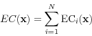
Under both, the unilateral and bilateral approaches, CVA is measured at the counterparty level. However, it is sometimes desirable to determine contributions of individual trades to the counterparty-level CVA. The problem of calculating CVA contributions bears many similarities to the calculation of risk contributions and capital allocation (see Aziz and Rosen 2004, Mausser and Rosen 2007). There are several possible measures of CVA contributions. We refer to the CVA of each transaction on a stand-alone basis as the transaction's stand-alone CVA. Clearly, when the given portfolio does not allow for netting between trades, the portfolio-level CVA is given by the sum of the individual trades' stand-alone CVA. However, this is not the case when netting and margin agreements are in place. We refer to the incremental CVA contribution of a trade as the difference between the portfolio CVA with and without the trade.6 This measure is commonly seen as appropriate for pricing counterparty risk for new trades with the counterparty (see Chapter 6 in Arvanitis and Gregory, 2001 for details). One problem with incremental CVA contributions is that they are non-additive - the sum of the individual trade's CVA contributions does not add up to the portfolio's CVA. Hence neither stand-alone nor incremental contributions can be used effective contributions of existing trades in the portfolio to the counterparty-level CVA, in the presence of netting and/or margin agreements. For this purpose we require additive CVA contributions. In this case, we draw the analogy with the capital allocation literature and refer to these as (continuous) marginal risk contributions.
The marginal CVA contributions with a given counterparty give the bank a clear picture how much each trade contributes to the counterparty-level CVA. However, the use of CVA contributions is not limited to an analysis at a single counterparty level. Once the CVA contributions have been calculated for each counterparty, the bank can calculate the price of counterparty credit risk in any collection of trades without any reference to the counterparties. For example, by selecting all trades booked by a certain business unit or product type (e.g., all CDSs or all USD interest rate swaps), the bank can determine the contribution of that business unit or product to the bank's total CVA.
We show how to define and calculate marginal CVA contributions in the presence of netting and margin agreements, and under a wide range of assumptions, including the dependence of exposure on the counterparty's credit quality. The theory of marginal risk contributions, sometimes refer to as Euler Allocations (see Tasche 2008), is now well developed and largely relies on the risk function being homogeneous (of degree one). We show that this principle can be applied readily for CVA when the counterparty portfolio allows for netting (but does not include collateral and margins). We further extend this allocation principle for the more general case of collateralized/margined counterparties For the sake of simplicity, we assume the unilateral framework throughout the paper. However, an extension of all the results to the bilateral framework is straightforward.
The paper is organized as follows. In Section 2, we define counterparty credit exposure for both collateralized and non-collateralized cases. We show how counterparty-level CVA can be calculated from the profile of the discounted risk neutral expected exposure (EE) conditional on the counterparty's default. In Section 3, we introduce CVA contributions of individual trades and relate them to the profiles of conditional EE contributions. In Section 4, we adapt the continuous marginal contribution (CMC) method often used for allocating economic capital to calculating EE contributions for the case when the counterparty-level exposure is a homogeneous function of the trades' weights in the portfolio. This is the case when there are no exposure-limiting agreements, such as margin agreements, with the counterparty. When such agreements are present, the CMC method fails because the counterparty-level exposure is not homogeneous anymore. In Section 5, we propose an EE allocation scheme that is based on the CMC method, but can be used for collateralized counterparties. In Section 6, we show how to incorporate EE and CVA contribution calculations into exposure simulation process. In Section 7, we derive closed form expressions for EE contributions under the assumption that all trade values are normally distributed. We start with the case of independence between exposure and the counterparty's credit quality, and extend the results to incorporate dependence between them (wrong-way risk). We also provide an intuitive explanation to our closed-form results. In Section 8, we show several numerical examples that illustrate the behavior of exposure (and hence CVA) contributions for both, the collateralized and non-collateralized cases.
2 Counterparty credit risk and CVA
In this section, we review the basic concepts and notation for counterparty credit risk, credit exposures and CVA.
Counterparty credit risk (CCR) is the risk that the counterparty defaults before the final settlement of a transaction's cash flows. An economic loss occurs if the counterparty portfolio has a positive economic value for the bank at the time of default. Unlike a loan,
where only the lending bank faces the risk of loss, CCR creates a bilateral risk: the market value can be positive or negative to either counterparty and can vary over time with the underlying market factors. We define the counterparty exposure ![]() of the bank to a counterparty at time
of the bank to a counterparty at time ![]() as the economic loss, incurred on all outstanding
transactions with the counterparty if the counterparty defaults at
as the economic loss, incurred on all outstanding
transactions with the counterparty if the counterparty defaults at ![]() , accounting for netting and collateral but unadjusted by possible recoveries.
, accounting for netting and collateral but unadjusted by possible recoveries.
2.1 Counterparty exposures
Consider a portfolio of ![]() derivative contracts of a bank with a given counterparty. The maturity of the longest contract in the portfolio is
derivative contracts of a bank with a given counterparty. The maturity of the longest contract in the portfolio is ![]() . The counterparty defaults at a random time
. The counterparty defaults at a random time ![]() with a known risk-neutral distribution
with a known risk-neutral distribution
![]() .7 We further assume
that the distribution of the trade values at all future dates is risk neutral.8
.7 We further assume
that the distribution of the trade values at all future dates is risk neutral.8
Denote the value of the ![]() th instrument in the portfolio at time
th instrument in the portfolio at time ![]() from the bank's
perspective by
from the bank's
perspective by ![]() . At each time
. At each time ![]() , the counterparty-level exposure
, the counterparty-level exposure ![]() is determined by the values of all trades with the counterparty at time
is determined by the values of all trades with the counterparty at time ![]() ,
,
![]() . The value of the counterparty portfolio at
. The value of the counterparty portfolio at ![]() is given
by
is given
by
For a counterparty portfolio with a single netting agreement, the (netted) exposure is
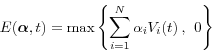
When the netting agreement is further supported by a margin agreement, the counterparty must provide the bank with collateral whenever the portfolio value exceeds a threshold. As the portfolio value drops below the threshold, the bank returns collateral to the counterparty. Collateral transfer occurs only when the collateral amount that needs to be transferred exceeds a minimum transfer amount. The counterparty-level (margined) exposure is given by
where
Counterparty portfolios with a combination of multiple netting agreements and trades outside of these agreements can be modeled in a straightforward way by a combination of Equations (2)-(4).
2.2 Models of Collateral
We start modeling collateral with a simplifying assumption: we incorporate the minimum transfer amount into the threshold ![]() and treat the margin agreement as having no minimum transfer
amount. This approximation is rather crude, but it is very popular amongst banks because it greatly simplifies modeling.
and treat the margin agreement as having no minimum transfer
amount. This approximation is rather crude, but it is very popular amongst banks because it greatly simplifies modeling.
We consider two models of collateral. In the instantaneous collateral model, we assume that collateral is delivered immediately and that the trades can be liquidated immediately as well. Under these simplifying assumptions, the collateral available to the bank
is
A more realistic collateral model must account for the time lag between the last margin call made before default and the settling of the trades with the defaulting counterparty. This time lag, which we denote by![]() , is known as the margin period of risk. While the margin period of risk is not known with certainty, we follow the standard practice and assume that it is a deterministic quantity that is defined at the margin agreement
level.10 We assume that the collateral available to the bank at time
, is known as the margin period of risk. While the margin period of risk is not known with certainty, we follow the standard practice and assume that it is a deterministic quantity that is defined at the margin agreement
level.10 We assume that the collateral available to the bank at time ![]() is determined by the portfolio value at time
is determined by the portfolio value at time ![]() according to
according to
2.3 Credit losses and CVA
In the event that the counterparty defaults at time ![]() , the bank recovers a fraction
, the bank recovers a fraction ![]() of the exposure
of the exposure ![]() . The bank's discounted loss due to the counterparty's default is
. The bank's discounted loss due to the counterparty's default is
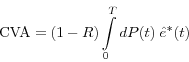
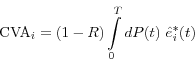
The unilateral counterparty-level CVA is obtained by applying the expectation to Equation (7). This results in
Throughout this paper we use "star" to designate discounting and "hat" to designate conditioning on default at time
3 CVA Contributions from EE Contributions
We would like to develop a general approach to calculating additive contributions of individual trades to the counterparty-level CVA. We denote the contribution of trade ![]() by
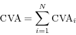
by ![]() . We say that CVA contributions are additive when they sum up to the counterparty-level CVA:
. We say that CVA contributions are additive when they sum up to the counterparty-level CVA:
and the CVA contribution of trade
Thus, from now on we focus on defining and calculating EE contributions.
Note first that, without netting agreements, the allocation of the counterparty-level EE across the trades is trivial because the counterparty-level exposure is the sum of the stand-alone exposures (Equation (2)) and expectation is a linear operator. Furthermore, when there is more than one netting set with the counterparty (e.g., multiple netting agreements, non-nettable trades), we can focus on first calculating the CVA contribution of a transaction to its netting set. The allocation of the counterparty-level EE across the netting sets is then trivial again because the counterparty-level exposure is defined as the sum of the netting-set-level exposures. Thus, our goal is to allocate the netting-set-level exposure to the trades belonging to that netting set. To keep the notation simple, we assume from now on that all trades with the counterparty are covered by a single netting set.
4 Additive EE Contributions for Non-collateralized Netting Sets
In this section, we develop the basic methodology to compute EE contributions and allocate portfolio-level EE for non-collateralized netting sets.
4.1 Continuous Marginal Contributions and Euler Allocation
We derive EE contributions by adapting the continuous marginal contributions (CMC) method from the economic capital (EC) literature. EC is calculated at the portfolio level and then it is allocated to individual obligors and transactions. Under the CMC method, the risk contribution of a given transaction to the portfolio EC is determined by the infinitesimal increment of the EC corresponding to the infinitesimal increase of the transaction's weight in the portfolio (see Chapter 4 in Arvanitis and Gregory (2001) or Tasche (2008) for details). This follows from the fact that the risk function is homogeneous (of degree one) and the application of Euler's theorem.
A real function ![]() of a vector
of a vector ![]() is said to be homogeneous of degree
is said to be homogeneous of degree ![]() if for all
if for all ![]() ,
, ![]() . If the function
. If the function ![]() is piecewise differentiable, then Euler's theorem states that:
is piecewise differentiable, then Euler's theorem states that:
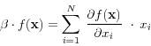
If ![]() denotes the vector of positions in a portfolio, and
denotes the vector of positions in a portfolio, and ![]() the corresponding economic capital, then Euler's theorem implies additive capital contributions
the corresponding economic capital, then Euler's theorem implies additive capital contributions
are referred to as the marginal capital contributions of the portfolio.
4.2 Continuous Marginal EE Contributions for netted exposures without collateral
Consider now the calculation of EE contributions. Assume that we can adjust the size of any trade in the portfolio by any amount. Define the weight ![]() for trade
for trade ![]() as a scale factor that represents the relative size of the trade in the portfolio,
as a scale factor that represents the relative size of the trade in the portfolio,
![]() . These weights can assume any real value, with
. These weights can assume any real value, with ![]() corresponding to the actual size of the trade and
corresponding to the actual size of the trade and ![]() being the complete removal of the trade. We describe adjusted portfolios via the vector of weights
being the complete removal of the trade. We describe adjusted portfolios via the vector of weights
![]() . For adjusted portfolios, we use the notations
. For adjusted portfolios, we use the notations
![]() ,
,
![]() , and
, and
![]() for the exposure and EE at time
for the exposure and EE at time ![]() and CVA. Furthermore, for
convenience, denote by
and CVA. Furthermore, for
convenience, denote by
![]() the vector representing the original portfolio.
the vector representing the original portfolio.
When there is no margin agreement between the bank and the counterparty, the counterparty-level exposure is a homogeneous function of degree one in the trade weights:
We define the continuous marginal EE contribution of trade ![]() at time
at time ![]() as the infinitesimal increment of the conditional discounted EE of the actual portfolio at time
as the infinitesimal increment of the conditional discounted EE of the actual portfolio at time ![]() resulting from an infinitesimal increase of trade
resulting from an infinitesimal increase of trade ![]() 's presence in the portfolio, scaled to the full trade amount:
's presence in the portfolio, scaled to the full trade amount:
We can derive an expression for the marginal EE contributions as follows. First, substitute Equation (9) into Equation (17) and bring the derivative inside the expectation. This results in
Calculating the first derivative of the exposure with respect to the weight
Substituting Equation (20) into Equation (18), we obtain the EE contribution of trade
The EE contribution of trade
![\begin{displaymath} \sum\limits_{i=1}^N {\hat {e}_i^\ast (t)} =\hat {E}_t \left[ {D(t){\kern 1pt}{\kern 1pt}V(t){\kern 1pt}{\kern 1pt}{\kern 1pt}{\bf 1}_{\{V(t)>0\}} } \right]=\hat {E}_t \left[ {D(t){\kern 1pt}{\kern 1pt}\max \left\{ {V(t),0} \right\}} \right]=\hat {e}^\ast (t) \end{displaymath}](img68.gif)
5 Additive EE Contributions for Collateralized Netting Sets
Consider now a counterparty that has a single netting agreement supported by a margin agreement, which covers all the trades with the counterparty. As discussed in Section 2, the counterparty-level stochastic exposure is given by Equation (4), where the collateral available to the bank is given either by the instantaneous collateral model (Equation (5)) or by the lagged collateral model (Equation (6)). In what follows, we specify additive EE contributions for both models, starting with the simpler instantaneous collateral model.
5.1 Instantaneous Collateral Model
Substituting Equation (5) into Equation (4), we obtain
We can derive additive contributions for this non-homogeneous case, which are consistent with the continuous marginal contributions as follows. First, notice that, while the exposure function in Equation (22) is not homogeneous in the vector of weights ![]() , the function
, the function
The first derivatives of the exposure with respect to the trade weights is given by
Note that these sum up to the counterparty-level exposure given by Equation (22), as expected. By applying discounting and taking conditional expectation of the right-hand side of Equations (24) and (25), we obtain the EE contributions of the trades
and of the threshold
which satisfy
The contribution of the threshold can be interpreted as the change of the conditional discounted EE associated with an infinitesimal shift of the threshold upwards scaled up by the actual size of the threshold. Note that, when the threshold goes to infinity, the last term vanishes and we recover the uncollateralized contributions.
As the final step, we "allocate back" the contribution adjustment of the collateral threshold given by Equation (27) to the individual trades, so that Equation (28) can be written in terms of EE contributions only of the trades (as in Equation (11)):
There are several possibilities for allocating the amount
Thus, the individual trade contributions to EE are given by
![\begin{displaymath} \;\hat {E}_t \,\left[ {D(t)\cdot 1_{\left\{ {V(t)>H} \right\}} } \right]\mbox{ }=\sum\limits_{i=1}^N {{\kern 1pt}{\kern 1pt}{\kern 1pt}\hat {E}_t \,\left[ {D(t)\cdot 1_{\left\{ {V(t)>H} \right\}} } \right]\,\,\cdot \,\,\frac{\hat {E}_t \,\left[ {D(t)\cdot V_i (t)\cdot 1_{\left\{ {V(t)>H} \right\}} } \right]}{\hat {E}_t \,\,\left[ {D(t)\cdot V(t)\cdot 1_{\left\{ {V(t)>H} \right\}} } \right]}} \end{displaymath}](img78.gif)
Both terms of Equation (30) have a straightforward interpretation: the first term is the contribution of all scenarios where the bank holds no collateral at time
We refer to the allocation scheme above as type A allocation. An alternative allocation scheme (type B) is obtained by bringing the weighting scheme of the threshold contribution now inside the expectation operator, so that instead of Equation (29) we now have:
![\begin{displaymath} \hat {E}_t \,\left[ {D(t)\cdot 1_{\left\{ {V(t)>H} \right\}} } \right]\mbox{ }=\sum\limits_{i=1}^N {{\kern 1pt}{\kern 1pt}\hat {E}_t \left[ {D(t)\cdot 1_{\left\{ {V(t)>H} \right\}} \cdot \;\frac{\sum\nolimits_{i=1}^N {V_i (t)} }{V(t)}} \right]\,} =\sum\limits_{i=1}^N {{\kern 1pt}{\kern 1pt}\hat {E}_t \left[ {D(t)\cdot \frac{V_i (t)}{V(t)}\cdot 1_{\left\{ {V(t)>H} \right\}} } \right]\,\,} \end{displaymath}](img80.gif)
Both terms on the right hand of Equation (32) have the same interpretation as before.
5.2 Lagged Collateral Model
We now apply the formalism developed for the continuous collateral model to the lagged collateral model. In this case, the counterparty credit exposure is obtained by substituting Equation (6) into Equation (4):
As defined for the instantaneous model, we rewrite the exposure given by Equation (33) as a homogeneous function in the extended vector of weights ![]() :
:
and
The sum these first derivatives across all the trades and the threshold, gives the counterparty-level exposure, Equation (33). By applying discounting and taking the conditional expectation of the right-hand side of Equations (36) and (37), we obtain the EE contributions of the trades
and of the threshold
Now we need to allocate back the threshold contribution, Equation (39), to the individual trades. Following the type A allocation scheme in the previous section,
In the type B allocation, we bring the weighting scheme inside the expectation operator. This gives
![\begin{displaymath} \begin{array}{c} \hat {e}_i^\ast (t)=\hat {E}_t \,\left[ {D... ...{ {0<H+\delta V(t)<V(t)} \right\}} } \right]} \ \end{array}\end{displaymath}](img92.gif)
It is straightforward to verify that the lagged EE contributions degenerate to the instantaneous EE contributions when
![\begin{displaymath} \begin{array}{c} \hat {e}_i^\ast (t)=\hat {E}_t \,\left[ {D(t)\cdot V_i (t)\cdot 1_{\left\{ {0<V(t)\le H+\delta V(t)} \right\}} } \right]+\hat {E}_t \,\left[ {D(t)\cdot \delta V_i (t)\cdot 1_{\left\{ {0<H+\delta V(t)<V(t)} \right\}} } \right] \ +H\cdot \hat {E}_t \,\left[ {D(t)\cdot \frac{V_i (t)}{V(t)}\cdot 1_{\left\{ {0<H+\delta V(t)<V(t)} \right\}} } \right] \ \end{array}\end{displaymath}](img93.gif)
6 Calculating CVA Contributions by Simulation
Banks commonly use Monte Carlo simulation in practice to obtain the distribution of counterparty-level exposures. Based on these simulations a bank can also compute the counterparty-level CVA. In this section, we show how the calculation of EE contributions can be easily incorporated to the Monte Carlo simulation of the counterparty-level exposure that banks already perform.
6.1 Exposure Independent of Counterparty's Credit Quality
Consider first the case where the exposures are independent of the counterparty's credit quality. In general, banks implicitly assume that each counterparty's exposure is independent of that counterparty's credit quality when exposures are simulated separately. Let us now make this assumption explicitly. Then, conditioning on ![]() in the expectations in Equations (19), (29), (30) and (32) become unconditional, and these conditional expectations can be replaced by the unconditional ones.
in the expectations in Equations (19), (29), (30) and (32) become unconditional, and these conditional expectations can be replaced by the unconditional ones.
The simulation algorithm for calculating counterparty-level CVA can be extended to calculate CVA contributions. For the ease of exposition, we assume that all the trades with the counterparty are nettable and that collateral (if there is any) can be described by the instantaneous model.
First, the counterparty-level CVA can be calculated in a Monte Carlo simulation as follows:
- Generate a market scenarios
 (interest rates, FX rates, etc.) for each of the future time points
- For each simulation time point and scenario :
- For each trade
 , calculate trade value
- Calculate portfolio value
- If there is margin agreement, calculate collateral
 available at time .
 - Calculate counterparty-level exposure
 (if there is no margin agreement,
  .
.
- For each trade
- After running large enough number
 of market scenarios, compute the discounted EE by averaging over all the market scenarios at each time point:
- Finally, compute CVA as
where, as before,
The calculation of EE and CVA contributions can be incorporated to this algorithm as follows. Consider, for example, the EE contributions given by Equation (32). The following calculations are added to Steps 2-4:
- Step 2: For each trade , calculate the trade's exposure contribution for scenario
 , which is equal to
  if
if  ,
,  if
if  , and zero otherwise.
 - Step 3: For each trade , compute the discounted EE contribution by averaging over all the market scenarios at each time point:
- Step 4: CVA contributions are computed as
6.2 Exposure Dependent on Counterparty's Credit Quality
The algorithm above assumes independence between the exposure and the counterparty's credit quality. More generally, there may be dependence between them which can come from two sources:
- Right/wrong-way risk. The risk is called right-way (wrong-way) if exposure tends to decrease (increase) when counterparty quality worsens. Strictly speaking, right/wrong-way risk is always present, but it is usually ignored to simplify exposure modeling. However, there are cases when right/wrong way risk is too significant to be ignored (e.g., credit derivatives, commodity trades with a producer of that commodity, etc.).
- Exposure-limiting agreements that depend on the counterparty credit quality. One example such agreements is a margin agreement with the threshold dependent on the counterparty's credit rating. Another example is an early termination agreement, under which the bank can terminate the trades with the counterparty when the counterparty's rating falls below a pre-specified level.
Let us introduce a stochastic default intensity process ![]() without specifying its underlying dynamics.11 This intensity can be used as a measure of counterparty credit quality: higher values of the intensity correspond to lower credit quality. The counterparty-level exposure
without specifying its underlying dynamics.11 This intensity can be used as a measure of counterparty credit quality: higher values of the intensity correspond to lower credit quality. The counterparty-level exposure ![]() may depend either on the intensity value
may depend either on the intensity value ![]() at time
at time ![]() , or on the entire path of the intensity process
, or on the entire path of the intensity process
![]() from zero to
from zero to ![]() . We can use the intensity process to convert the
expectation conditional on default at time
. We can use the intensity process to convert the
expectation conditional on default at time ![]() in Equation (21) to an unconditional expectation so that the conditional EE contribution becomes
in Equation (21) to an unconditional expectation so that the conditional EE contribution becomes
![\begin{displaymath} \hat {e}_i^\ast (t)=\frac{1}{{P}'(t)}E\left[ {\lambda (t)\exp \left( {-\int\limits_0^t {\lambda (s)ds} } \right){\kern 1pt}{\kern 1pt}D(t){\kern 1pt}E_i (t){\kern 1pt}} \right] \end{displaymath}](img116.gif)
As described for unconditional EE contributions, the calculations for conditional EE contributions can be performed during a Monte Carlo simulation of exposures. In this case, given the dependence of exposures on the counterparty credit quality, the intensity process
![]() needs to be simulated jointly with the market risk factors that determine trade values. This joint simulation is done path-by-path: simulated values of the intensity and of
the market factors at time
needs to be simulated jointly with the market risk factors that determine trade values. This joint simulation is done path-by-path: simulated values of the intensity and of
the market factors at time ![]() are obtained from the corresponding simulated values at the earlier time points (
are obtained from the corresponding simulated values at the earlier time points (
![]() .12 Assuming that we have
already simulated the market factors and the intensity for times
.12 Assuming that we have
already simulated the market factors and the intensity for times ![]() for all
for all ![]() , the algorithm for computing CVA contributions for time
, the algorithm for computing CVA contributions for time ![]() can be expressed as follows:
can be expressed as follows:
- Jointly simulate market risk factors and intensity
 at time
 - For each trade , calculate its trade value

- Calculate the portfolio value
- For each trade , update the EE contribution counter
- If there is no margin agreement, then
- if
 , add
, add
- if
- If there is a margin agreement with an intensity-dependent threshold
![h[\lambda (\cdot )]](img126.gif) , then
, then
- if
![0<V(t)\le h[\lambda (t_k )]](img127.gif) , add
, add
- if
![V(t)>h[\lambda (t_k )]](img128.gif) , add
, add
![\frac{\lambda (t_k )}{{P}'(t_k )}\exp \left( {-\sum\nolimits_{j=1}^k {\lambda (t_{j-1} )(t_j -t_{j-1} )} } \right)D(t_k )h[\lambda (t_k )]\frac{V_i (t_k )}{V(t_k )}](img129.gif)
- if
- If there is no margin agreement, then
7 Analytical CVA Contributions under a Normal Approximation
It is also useful in practice to estimate EE and CVA contributions quickly outside of the simulation system. To facilitate such calculations, we derive analytical EE contributions, for the case when trade values are normally distributed. For simplicity, and to avoid dealing with stochastic
discounting factors, we assume that, at time ![]() the distribution of trade values is given under the forward (to time
the distribution of trade values is given under the forward (to time ![]() probability measure. Under this measure, the discounted conditional EE in Equation (9) can be written as
probability measure. Under this measure, the discounted conditional EE in Equation (9) can be written as
where
Assume that the value ![]() of trade
of trade ![]() at each future time
at each future time ![]() is normally distributed with expectation
is normally distributed with expectation ![]() and standard deviation
and standard deviation ![]() under the forward to
under the forward to ![]() probability measure:
probability measure:
Since the sum of normal variables is also normal, the discounted portfolio value ![]() is normally distributed:
is normally distributed:
Denote by
Using this correlation, we can represent
![\begin{displaymath} \rho _i (t)=\frac{cov[V_i (t),V(t)]}{\sigma _i (t){\kern 1pt}{\kern 1pt}{\kern 1pt}\sigma (t)}=\frac{\sum\nolimits_{j=1}^N {cov[V_i (t),V_j (t)]} }{\sigma _i (t){\kern 1pt}{\kern 1pt}{\kern 1pt}\sigma (t)}=\sum\limits_{j=1}^N {{\kern 1pt}{\kern 1pt}{\kern 1pt}{\kern 1pt}{\kern 1pt}r_{ij} \frac{\sigma _j (t)}{\sigma (t)}{\kern 1pt}} \end{displaymath}](img145.gif)
where
7.1 Exposure Independent of Counterparty's Credit Quality
We first calculate counterparty-level EE and EE contributions assuming independence between exposures and counterparty credit quality. We obtain the results for the general case of a netting agreement with a margin agreement. The simpler case, with no margin agreement, is obtained as the limiting case when the threshold goes to infinity. For the clarity of exposition, we assume the instantaneous collateral model.
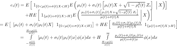
In the presence of a margin agreement, the counterparty-level stochastic exposure is given by Equation (22). Substituting Equation (46) into Equation (22) and taking the expectation, we obtain
![\begin{displaymath} \begin{array}{c} e(t)=E\left[ {\left[ {\mu (t)+\sigma (t)X} \right]{\kern 1pt}{\kern 1pt}{\kern 1pt}{\kern 1pt}1_{\left\{ {0<\mu (t)+\sigma (t)X<H} \right\}} } \right]+HE\left[ {{\kern 1pt}{\kern 1pt}1_{\left\{ {\mu (t)+\sigma (t)X>H} \right\}} } \right] \ =\int\limits_{-\frac{\mu (t)}{\sigma (t)}}^{\frac{H-\mu (t)}{\sigma (t)}} {\left[ {\mu (t)+\sigma (t)x} \right]\phi (x)dx} +H\int\limits_{\frac{H-\mu (t)}{\sigma (t)}}^\infty {\phi (x)dx} \ \end{array}\end{displaymath}](img148.gif)
where
where
![\begin{displaymath} \begin{array}{c} e(t)=\mu (t){\kern 1pt}{\kern 1pt}\left[ {\Phi \left( {\frac{\mu (t)}{\sigma (t)}} \right)-\Phi \left( {\frac{\mu (t)-H}{\sigma (t)}} \right)} \right] \ +\sigma (t){\kern 1pt}{\kern 1pt}{\kern 1pt}\left[ {\phi \left( {\frac{\mu (t)}{\sigma (t)}} \right)-\phi \left( {\frac{\mu (t)-H}{\sigma (t)}} \right)} \right]+H\Phi \left( {\frac{\mu (t)-H}{\sigma (t)}} \right) \ \end{array}\end{displaymath}](img150.gif)
Let us consider now the EE contributions given by Equation (32) (type B allocations). Removing the discounting and substituting Equations (45) and (46) into Equation (32), we obtain
where the remaining integral can be easily evaluated numerically. One can verify that EE contributions given by Equation (52) sum up to the counterparty-level EE, Equation (50).
Similarly, we obtain the EE contributions corresponding to type A allocations as
For the case without a margin agreement, we take the limit ![]() of Equations (50)-(53). This leads to the counterparty-level EE
of Equations (50)-(53). This leads to the counterparty-level EE
7.2 Right/Wrong-Way Risk
We now lift the independence assumption to accommodate right/wrong-way risk. Note that the EE contributions obtained in the previous section are contributions of the trades in the portfolio to the counterparty-level unconditional discounted EE. We need to modify the approach to obtain the contributions to the counterparty-level EE conditional on the counterparty defaulting at the time when the exposure is measured. An obvious approach is to define an intensity process and compute the conditional EE contributions as the expectation over all possible paths of the intensity process (See Appendix 1), but this requires a Monte Carlo simulation. In this section, we develop an alternative, simpler approach that results in closed form expressions for the conditional EE contributions.
For this purpose, we define a Normal copula13 to model the codependence between the counterparty's credit quality and the exposures.14 Thus, we first map the counterparty's default time ![]() to a standard normal random variable
to a standard normal random variable ![]() :
:
while the conditional EE contribution of trade
where
We model the right/wrong-way risk by allowing trade values to depend on
where
If the portfolio contains trades with non-zero ![]() , the standard normal risk factor
, the standard normal risk factor ![]() , which drives the portfolio value, also depends on
, which drives the portfolio value, also depends on ![]() :
:
Now we have all the ingredients to derive the counterparty-level EE and EE contributions in the presence of right/wrong-way risk. One approach may be to calculate conditional expectations in the same manner as we have calculated the unconditional ones in the previous Section. However, in Appendix 2 we show how this can be done in a faster and more elegant way. In particular, the conditional exposure model can be formulated the in exactly the same mathematical terms as the unconditional model. The only difference is that instead of the unconditional expectations, standard deviations and correlations that specify the behavior of the trade values, we now use the conditional ones. Therefore, we can use all the results of Subsection 7.1 (Equations (50)-(55)) after putting "hats" on the parameters: 15
![\begin{displaymath} \beta (t)=cov[X,Y]=\frac{cov[V(t),Y]}{\sigma (t)}=\sum\limits_{i=1}^N {\frac{cov[V_i (t),Y]}{\sigma (t)}} =\sum\limits_{i=1}^N {b_i \frac{\sigma _i (t)}{\sigma (t)}} \end{displaymath}](img176.gif)
7.3 Remarks on the Analytical Formulae
In this section we briefly comment on the properties and interpretation of the analytical contributions derived in this section.
Netting & no margin
Equation (55) can be understood from the incremental viewpoint of the CMC method. According to Equation (17), the EE contribution of trade ![]() is
determined by the infinitesimal change of the counterparty-level EE resulting from an infinitesimal increase of the weight of trade
is
determined by the infinitesimal change of the counterparty-level EE resulting from an infinitesimal increase of the weight of trade ![]() in the portfolio. The effect of an increase of the weight of
a trade on the portfolio value distribution can be viewed as the sum of two effects:
in the portfolio. The effect of an increase of the weight of
a trade on the portfolio value distribution can be viewed as the sum of two effects:
- a uniform shift of the distribution
- a change of width of the distribution
If the weight of trade ![]() is increased by
is increased by ![]() , the expectation of portfolio
value changes by
, the expectation of portfolio
value changes by
![]() . Let us first ignore the change of the standard deviation and consider how a uniform shift of the entire distribution by
. Let us first ignore the change of the standard deviation and consider how a uniform shift of the entire distribution by
![]() affects the counterparty-level EE. Scenarios with positive portfolio value contribute the same amount
affects the counterparty-level EE. Scenarios with positive portfolio value contribute the same amount
![]() to the exposure change, while scenarios with negative portfolio value contribute nothing. Therefore, the increment of the EE will be given by the product of the
magnitude of the shift
to the exposure change, while scenarios with negative portfolio value contribute nothing. Therefore, the increment of the EE will be given by the product of the
magnitude of the shift
![]() and the probability of the portfolio value being positive. It is straightforward to verify that
and the probability of the portfolio value being positive. It is straightforward to verify that
![]() . Thus, the first term in the right-hand side of Equation (55) describes the increment of the
counterparty-level EE resulting from the infinitesimal uniform shift of the portfolio value distribution associated with an increase of the weight of trade
. Thus, the first term in the right-hand side of Equation (55) describes the increment of the
counterparty-level EE resulting from the infinitesimal uniform shift of the portfolio value distribution associated with an increase of the weight of trade ![]() .
.
The second term of Equation (55) describes the change of the width of the portfolio value distribution. The change of the standard deviation of the portfolio value resulting from increasing the weight of trade ![]() by
by ![]() can be calculated as
can be calculated as
![\begin{displaymath} \begin{array}{l} StDev[V(t)+\delta V_i (t)]-StDev[V(t)]=\left( {var[V(t)]+2\delta cov[V(t),V_i (t)]+\delta ^2var[V_i (t)]} \right)^{\frac{1}{2}}-\sigma (t) \ =\left( {\sigma ^2(t)+2{\kern 1pt}\delta {\kern 1pt}\rho _i (t){\kern 1pt}{\kern 1pt}\sigma _i (t){\kern 1pt}{\kern 1pt}\sigma (t)+\delta ^2var[V_i (t)]} \right)^{\frac{1}{2}}-\sigma (t)=\delta {\kern 1pt}{\kern 1pt}\rho _i (t){\kern 1pt}{\kern 1pt}\sigma _i (t){\kern 1pt}{\kern 1pt}+O(\delta ^2) \ \end{array}\end{displaymath}](img185.gif)
where
The second term of Equation (55) can be obtained by taking the expectation of the right-hand side of Equation (69).
It appears that Equation (55) has simple linear dependence on ![]() and the product
and the product
![]() . However, this is only part of the true dependence. Since trade
. However, this is only part of the true dependence. Since trade ![]() is part of the portfolio,
is part of the portfolio, ![]() depends on
depends on ![]() and
and ![]() depends on
depends on ![]() and the
correlation of trade
and the
correlation of trade ![]() with the rest of the portfolio. Moreover, correlation
with the rest of the portfolio. Moreover, correlation ![]() is the correlation between the values of trade
is the correlation between the values of trade ![]() and the portfolio that includes trade
and the portfolio that includes trade ![]() itself. Because of this,
itself. Because of this, ![]() depends on the ratio
depends on the ratio
![]() (see Equation (48)). Thus, unless trade
(see Equation (48)). Thus, unless trade ![]() represents a negligible fraction of the portfolio, the true dependence of EE contribution on trade parameters is non-linear.
represents a negligible fraction of the portfolio, the true dependence of EE contribution on trade parameters is non-linear.
Netting & margin
In this case, only the first two terms of Equation (52) allow interpretation from the incremental viewpoint of the CMC method: the first term can be explained as the effect of the uniform shift and the second term as the effect of the widening or narrowing of the portfolio
value distribution. The third term results from the allocation of exposure when the portfolio value is above the threshold. An attempt to use the CMC method would give zero EE contribution from ![]() scenarios.
scenarios.
Equation (52) can be re-written as
![\begin{displaymath} \begin{array}{c} e_i (t)=\mu _i (t){\kern 1pt}{\kern 1pt}\l... ...\xi d\xi }{\mu (t)+\sigma (t)\xi }} } \right] \ \end{array}\end{displaymath}](img196.gif)
Right/wrong-way risk
If the value of trade ![]() is correlated with the counterparty's credit quality, its value distribution at time
is correlated with the counterparty's credit quality, its value distribution at time ![]() conditional on the counterparty's default at time
conditional on the counterparty's default at time ![]() differs from its unconditional value distribution. If the correlation is positive (right-way risk), the
distribution shifts down; if the correlation is negative (wrong-way risk), the distribution shifts up. In both cases, the distribution becomes narrower. Under the normal approximation, the shift of the distribution is described by Equation (64), and the narrowing is described by
Equation (65).
differs from its unconditional value distribution. If the correlation is positive (right-way risk), the
distribution shifts down; if the correlation is negative (wrong-way risk), the distribution shifts up. In both cases, the distribution becomes narrower. Under the normal approximation, the shift of the distribution is described by Equation (64), and the narrowing is described by
Equation (65).
An interesting property of Equation (64) is its dependence on the counterparty's PD. To understand this, let us consider the bank entering into the same trade with an investment-grade counterparty A and with a speculative-grade counterparty B. We are interested in the trade value distribution conditional on the counterparty's default at the time of observation. For the case of wrong (right) way risk, the deterioration of the counterparty's credit quality to the point of default pushes trade values higher (lower). Since counterparty A is "further away" from default than counterparty B, the deterioration of credit quality to the point of default is larger for counterparty A. Therefore, trade values conditional on default of A are shifted more than trade values conditional on default of B. Note that this is not specific to the normal approximation, but is a general property not related to any model.
8 Examples
In this section, we present some simple examples that illustrate the behavior of exposure (and hence CVA) contributions. For ease of exposition, we assume that trade values are Normal, as well as market and credit independence. However, as discussed earlier in Section 7.2, the conclusions apply equally to the case of wrong-way risk by simply using conditional expectations, volatilities and correlations, instead of unconditional ones. We first present an example when there is no collateral agreement in place, and then show the impact of adding a collateral agreement to the portfolio.
8.1 Contributions for a Non-collateralized Portfolio
As a first step to understand this behavior, consider Equations (54) and (55), which give the counterparty-level EE and the EE trade contributions, in the case when there is no margin agreement in place:
![]()
The EE contribution of instrument ![]() is a function of:
is a function of:
- the mean value contribution,


- the volatility contribution,


- the overall value of the ratio
 (for the entire portfolio)
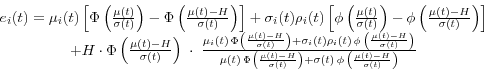
Both the counterparty-level EE and the trade contributions can be seen as the sum of two components: a mean value component (first term in the equations), and a volatility component (second term). These components weigh the mean value (or mean value contributions) and the volatility (volatility contribution), respectively, by the Normal distributions and density evaluated at the ratio ![]() (for the entire counterparty portfolio). Thus, the overall level of the counterparty portfolio's mean value and volatility determine how the individual instrument's mean and volatility contribution are weighted to yield the EE contributions. Figure 1 plots these weights as a function of
(for the entire counterparty portfolio). Thus, the overall level of the counterparty portfolio's mean value and volatility determine how the individual instrument's mean and volatility contribution are weighted to yield the EE contributions. Figure 1 plots these weights as a function of ![]() . A low ratio weighs the volatility contribution much higher; while a high ratio weighs mean values much more. For example, if
. A low ratio weighs the volatility contribution much higher; while a high ratio weighs mean values much more. For example, if ![]() = -2, the volatility component weight is 2.4 times the mean value weight. In contrast,
= -2, the volatility component weight is 2.4 times the mean value weight. In contrast, ![]() = 2 results in mean values being weighted 18 times the volatilities.
= 2 results in mean values being weighted 18 times the volatilities.
Figure 1: Volatility and mean exposure weights for EE contributions.
To illustrate the impact of various parameters on EE contributions, consider now the simple counterparty portfolio, which comprises of 5 transactions over a single step. Table 1 gives the individual trade's mean value, variance and volatility (in dollar values and % contributions). The portfolio has a mean value and variance of 10. We assume that trade values are independent.17 In this case, the portfolio's ratio ![]() = 3.16.
= 3.16.
| P1 | P2 | P3 | P4 | P5 | Total | |
|---|---|---|---|---|---|---|
| μ | 0 | 1 | 2 | 3 | 4 | 10 |
| μ (%) | 0% | 10% | 20% | 30% | 40% | 100% |
| σ 2 | 4 | 3 | 2 | 1 | 0 | 10 |
| σ 2 (%) | 40% | 30% | 20% | 10% | 0% | 100% |
| σ | 2 | 1.7 | 1.4 | 1.0 | 0.0 | 3.2 |
The portfolio is constructed so that for each trade, its mean value and volatility are inversely related; thus the first instrument, P1, has the lowest mean (0) and largest volatility (2), while position 5 has the highest mean value (4), and lowest volatility (0). This may not only be reasonably realistic, but it will also help highlight some of the points below.
Using Equations (54) and (55), we compute the EE and contributions for the portfolio. The EE for the portfolio is 10.001, with most of this arising from the mean value component (9.992). The trade contributions to EE are fairly close to the contributions to the mean values in Table 1 (0.03%, 10.02%, 20.00%, 29.98%, 39.97%).
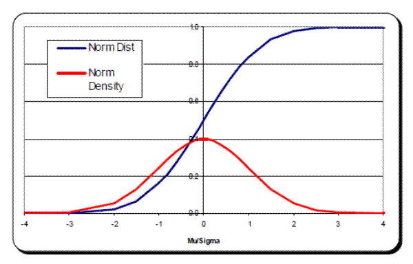
Now, we vary the overall mean value of the portfolio,![]() , while leaving intact the volatility,
, while leaving intact the volatility, ![]() , as well as the percent contributions of each instrument to the mean exposure and volatility in table 1. This allows us to express the trade contributions in terms of how deep in- or out-of-the-money the counterparty portfolio is (relative to its volatility). Figure 2 plots the EE, as well as its mean and volatility components, as functions of the portfolio's
, as well as the percent contributions of each instrument to the mean exposure and volatility in table 1. This allows us to express the trade contributions in terms of how deep in- or out-of-the-money the counterparty portfolio is (relative to its volatility). Figure 2 plots the EE, as well as its mean and volatility components, as functions of the portfolio's![]() . For large negative portfolio mean values, the EE (red line) is zero. In this case, the mean value component of EE is actually negative, and the volatility component compensates for this to generate positive EEs. As
. For large negative portfolio mean values, the EE (red line) is zero. In this case, the mean value component of EE is actually negative, and the volatility component compensates for this to generate positive EEs. As ![]() increases beyond zero, the volatility component decreases and, once
increases beyond zero, the volatility component decreases and, once ![]() 2, the EE is completely dominated by the mean value.
2, the EE is completely dominated by the mean value.
Figure 2. EE as a function of the portfolio's ratio μ/σ.
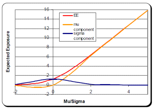
Figure 3 shows the EE contributions for each of the 5 trades as a function of ![]() . There is a clear shift in dominance between the mean and volatility components as the portfolio's mean value increases. At one side of the spectrum, when the mean portfolio values are negative, trades 4 and 5, which have the largest (negative) mean values and lowest volatilities, produce very large negative EE contributions. The opposite occurs for trades 1 and 2 (with low negative means and large volatilities). As the portfolio's
. There is a clear shift in dominance between the mean and volatility components as the portfolio's mean value increases. At one side of the spectrum, when the mean portfolio values are negative, trades 4 and 5, which have the largest (negative) mean values and lowest volatilities, produce very large negative EE contributions. The opposite occurs for trades 1 and 2 (with low negative means and large volatilities). As the portfolio's ![]() increases, trades 4 and 5 end up dominating the contributions, with the EE contribution converging to the mean value contributions themselves. For this particular symmetric portfolio, every trade contributes 20% of EE at
increases, trades 4 and 5 end up dominating the contributions, with the EE contribution converging to the mean value contributions themselves. For this particular symmetric portfolio, every trade contributes 20% of EE at ![]() = 0.506.
= 0.506.
Figure 3: EE Contributions as a function of the portfolio's ratio μ/σ.
8.2 Contributions for a Collateralized Portfolio
We consider now the case when there is a margin agreement, and demonstrate the impact of the collateral on the trade contributions. In very general terms:
- As the threshold becomes very large, trade contributions converge to those of uncollateralized exposures;
- With lower thresholds, the contributions of more volatile exposures are diminished (as the threshold caps the exposures), and contributions of higher mean exposures (in-the-money positions) increase.
Figure 4: EE reductions from a collateral agreement.
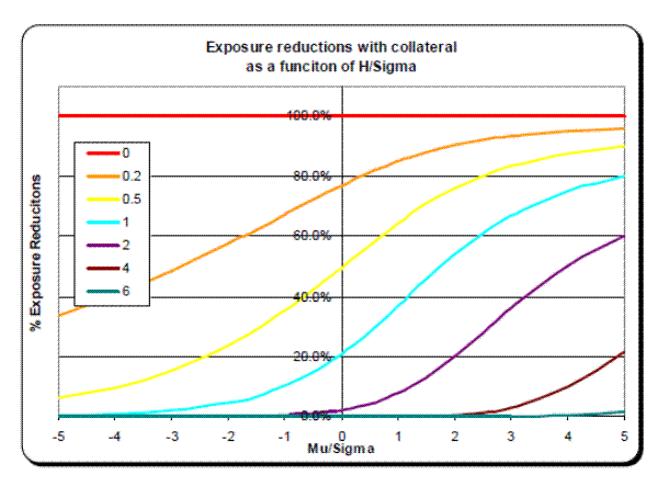
As the threshold is increased, the EE reductions decrease, as expected. Also, the collateral thresholds become more effective at reducing EE as the portfolio is deeper in-the-money (i.e. when ![]() increases). For example, a normalized threshold of 2 does not reduce EE until the portfolio's mean value is positive. At a value of
increases). For example, a normalized threshold of 2 does not reduce EE until the portfolio's mean value is positive. At a value of ![]() = 5, it reduces EE by about 60%.
= 5, it reduces EE by about 60%.
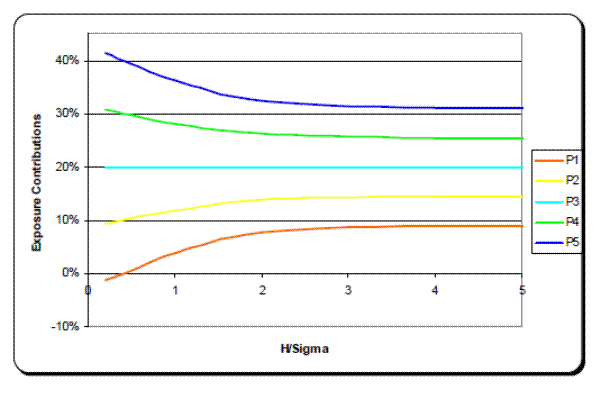
Figure 5 plots the EE contributions for the case ![]() = 1, as a function of the standardized threshold, H/
= 1, as a function of the standardized threshold, H/![]() . At high threshold values, H/
. At high threshold values, H/![]() > 4, trade contributions are essentially the uncollateralized contributions. Conversely at low H/
> 4, trade contributions are essentially the uncollateralized contributions. Conversely at low H/![]() values, EE contributions are basically the mean value contributions. The presence of the collateral affects each instrument's contributions differently. In particular, a tighter threshold increases the percent contributions of trades P4 and P5 (which have the highest mean values) while reducing the contributions of P1 and P2 (the lowest mean values). These eventually converge in the limit to the mean value contributions.
values, EE contributions are basically the mean value contributions. The presence of the collateral affects each instrument's contributions differently. In particular, a tighter threshold increases the percent contributions of trades P4 and P5 (which have the highest mean values) while reducing the contributions of P1 and P2 (the lowest mean values). These eventually converge in the limit to the mean value contributions.
Figure 5: EE contributions as a function of the collateral threshold.
Note finally that a trivial case arises when the ratio ![]() = 0. In this case, the EE contributions are independent of the threshold level H/
= 0. In this case, the EE contributions are independent of the threshold level H/![]() and equal the uncollateralized contributions.
and equal the uncollateralized contributions.
9 Conclusions
Counterparty credit risk is usually measured and priced at the counterparty level. The price of the counterparty risk for the entire portfolio of trades with a counterparty is known as credit valuation adjustment (CVA). In this article we have proposed a methodology for allocation of the counterparty-level CVA to individual trades. These allocations are additive, so that one can aggregate the CVA allocations for any collection of trades with different counterparties. Thus, the contribution of all trades belonging to a certain class to the bank-level CVA can be calculated. Such a class can be defined as "all trades booked by a certain business unit", "all EUR interest rate swaptions", etc.
In this paper, we show that the calculation of CVA allocations can be reduced to the calculation of contributions of individual trades to the counterparty-level expected exposure (EE) conditional on the counterparty's default. To obtain conditional EE contributions, we adapt the continuous marginal contribution method which is often used for allocating economic capital. The method is directly applicable for CVA contributions only when the counterparty-level exposure is a homogeneous function of the trades' weights in the portfolio. This is the case when there are no collateral or margin agreements. We extend the methodology to deal with non-homogeneous exposures of the type encountered when the portfolios have margin agreements.
We further show how the calculations of conditional EE contributions can be incorporated into an existing exposure simulation process. In addition, the ability to make quick calculations of CVA allocations outside of the exposure simulation system may be also desirable. To facilitate such calculations, we derive closed form expressions for unconditional EE contributions under the assumption that trade values are normally distributed. By using unconditional EEs in the CVA calculations, one implicitly assumes that exposures are independent of the counterparty credit quality. To overcome this limitation, we extend the results for conditional EE contributions in the normal approximation, which incorporate dependence between the trade values and the counterparty's credit quality.
Aziz A. and D. Rosen, 2004, Capital Allocation and RAPM, The Professional Risk Manager's Handbook (C. Alexander and E. Sheedy editors), PRMIA Publications, Wilmington, DE (www.prmia.org), pages 13-41.
A. Arvanitis and J. Gregory, 2001, "Credit: The Complete Guide to Pricing, Hedging and Risk Management", Risk Books
D. Brigo and M. Masetti, 2005, Risk Neutral Pricing of Counterparty Credit Risk in "Counterparty Credit Risk Modelling" (M. Pykhtin, ed.), Risk Books
E. Canabarro and D. Duffie, 2003, Measuring and Marking Counterparty Risk
in "Asset/Liability Management for Financial Institutions" (L. Tilman, ed.), Institutional Investor Books
Garcia Cespedes J. C., de Juan Herrero J. A., Rosen D., and Saunders D., 2009, Effective modelling of CCR Capital and Alpha for Derivatives Portfolios, Working Paper, Fields Institute and University of Waterloo
M. Gibson, 2005, Measuring Counterparty Credit Exposure to a Margined Counterparty in "Counterparty Credit Risk Modelling" (M. Pykhtin, ed.), Risk Books
D. Li, 2000, On Default Correlation: a Copula Approach, Journal of Fixed Income 9, pages 43-54.
H. Mausser and D. Rosen, 2007, Economic credit capital allocation and risk contributions, in Handbook of Financial Engineering, J. Birge and V. Linetsky, eds., vol. 15 of Handbooks in Operations Research and Management Science, North-Holland, 2007, pp. 681-726.
E. Picoult, 2005, Calculating and Hedging Exposure, Credit Value Adjustment and Economic Capital for Counterparty Credit Risk in "Counterparty Credit Risk Modelling" (M. Pykhtin, ed.), Risk Books
M. Pykhtin and S. Zhu, 2006, Measuring Counterparty Credit Risk for Trading Products under Basel II in "Basel Handbook", 2nd Edition (M. Ong, ed.), Risk Books
M. Pykhtin and S. Zhu, 2007, A Guide to Modeling Counterparty Credit Risk, GARP Risk Review, July/August, pages 16-22.
M. Pykhtin, 2009, Modeling Credit Exposures for Collateralized Counterparties, Journal of Credit Risk, 5(4).
C. Redon, 2006, Wrong Way Risk Modelling, Risk, April, pages 90-95.
P. Schönbucher (2003), "Credit Derivatives Pricing Models", Wiley Finance.
10 Appendix 1. Derivation of Equation (42)
Suppose we have a random variable ![]() and we want to calculate its expectation conditional on the counterparty defaulting at time
and we want to calculate its expectation conditional on the counterparty defaulting at time ![]() (
(![]() . We can express this expectation as
. We can express this expectation as
![\begin{displaymath} \begin{array}{c} E\left[ {W{\kern 1pt}{\kern 1pt}1_{\{t<\tau \le t+dt\}} } \right]=E\left[ {W\left( {\exp [-\int\limits_0^t {\lambda (s)ds} ]-\exp [-\int\limits_0^{t+dt} {\lambda (s)ds} ]} \right)} \right] \ =E\left[ {W\exp [-\int\limits_0^t {\lambda (s)ds} ]\left( {1-\exp [-\lambda (t)dt]} \right)} \right] \ =E\left[ {W\exp [-\int\limits_0^t {\lambda (s)ds} ]{\kern 1pt}{\kern 1pt}{\kern 1pt}\lambda (t)dt} \right] \ \end{array}\end{displaymath}](img209.gif)
For the denominator, we can write
where
![\begin{displaymath} E\left[ {\left. {W{\kern 1pt}{\kern 1pt}} \right\vert{\kern 1pt}{\kern 1pt}{\kern 1pt}{\kern 1pt}\tau {\kern 1pt}{\kern 1pt}={\kern 1pt}{\kern 1pt}t} \right]=\frac{1}{{P}'(t)}E\left[ {W{\kern 1pt}\lambda (t)\exp [-\int\limits_0^t {\lambda (s)ds} ]{\kern 1pt}{\kern 1pt}{\kern 1pt}} \right] \end{displaymath}](img211.gif)
11 Appendix 2. Analytical Results under Normal Approximation.
A2.1 Exposure Independent of Counterparty's Credit Quality
We derive now Equation (52) from Equation (51), which we restate here for convenience:
Substituting Equation (49) and inserting the expectation conditional on
While evaluating of the first integral is straightforward, there is no closed form solution for the second one. This results in Equation (42):
![\begin{displaymath} \begin{array}{c} e_i (t)=\mu _i (t){\kern 1pt}{\kern 1pt}\left[ {\Phi \left( {\frac{\mu (t)}{\sigma (t)}} \right)-\Phi \left( {\frac{\mu (t)-H}{\sigma (t)}} \right)} \right]+\sigma _i (t){\kern 1pt}\rho _i (t){\kern 1pt}{\kern 1pt}{\kern 1pt}\left[ {\phi \left( {\frac{\mu (t)}{\sigma (t)}} \right)-\phi \left( {\frac{\mu (t)-H}{\sigma (t)}} \right)} \right] \ +H\int\limits_{\frac{H-\mu (t)}{\sigma (t)}}^\infty {\frac{\mu _i (t)+\sigma _i (t)\rho _i (t)x}{\mu (t)+\sigma (t)x}\phi (x)dx} \ \end{array}\end{displaymath}](img153.gif)
A2.2 EE Contributions under Right/Wrong-way Risk
We present the derivation of the analytical EE contributions when exposures are correlated with the counterparty credit quality. Specifically, we show that we can use Equations (51)-(55), with the only difference that instead of using the unconditional expectations, standard deviations and correlations that specify the behavior of the trade values, we now use the conditional ones.
From conditional expectation to conditional random variables
The conditional expectation of a random variable can always be formulated as the unconditional expectation of a conditional random variable. For example, the counterparty-level conditional EE in Equation (59) can be represented as
where
Conditional trade values are calculated as follows. By substituting Equation (61) into Equation (45) and setting ![]() , we obtain the value
, we obtain the value ![]() of trade
of trade ![]() conditional on the counterparty defaulting at time
conditional on the counterparty defaulting at time ![]() :
:
and
The conditional portfolio value
where
and
Finally, we need the correlation between the conditional trade value and the conditional portfolio value. Let us denote the correlation between
where we have taken into account that both
Note that
where
Now we have formulated the conditional exposure model in exactly the same mathematical terms as the unconditional model of Section 7 and can use all the results of Subsection 7.1 after putting "hats" on the parameters!