
Structural Shocks and the Comovements
between Output and Interest Rates
Keywords: Interest rates, business cycles, structural VAR, bandpass filter, news shocks
Abstract:
Conditional on shocks to neutral technology and monetary policy, the results square with simple models, like the standard RBC model or a textbook version of the New Keynesian model. In addition, news about future productivity help to explain the overall counter-cyclical behavior of the real rate.
A sub-sample analysis documents also interesting changes in these pattern. During the Great Inflation (1959-1979), permanent shocks to inflation accounted for the counter-cyclical behavior of the real rate and its inverted leading indicator property. Over the Great Moderation (1982-2006), neutral technology shocks were more dominant in explaining comovements between output and interest rates, and the real rate has been pro-cyclical.
JEL Classification: C32, E32 and E43.
I Introduction
Understanding the relationship between output and interest rates is important to macroeconomists and policymakers alike. But basic stylized facts on their comovements in U.S. data have proved difficult to match within a variety of simple DSGE models. For instance, KingWatson:1996 study three models: a real business cycle model, a sticky price model, and a portfolio adjustment cost model. They report that this battery of modern dynamic models fails to match the business cycle comovements of real and nominal interest rates with output:
While the models have diverse successes and failures, none can account for the fact that real and nominal interest rates are "inverted leading indicators" of real economic activity.1
Calling interest rates inverted leading indicators refers to their negative correlation with future output. These correlations are typically measured once the series have been passed through a business cycle filter.2 Amongst the diverse failures mentioned by KingWatson:1996, RBC models generate mostly a pro-cyclical real rate.
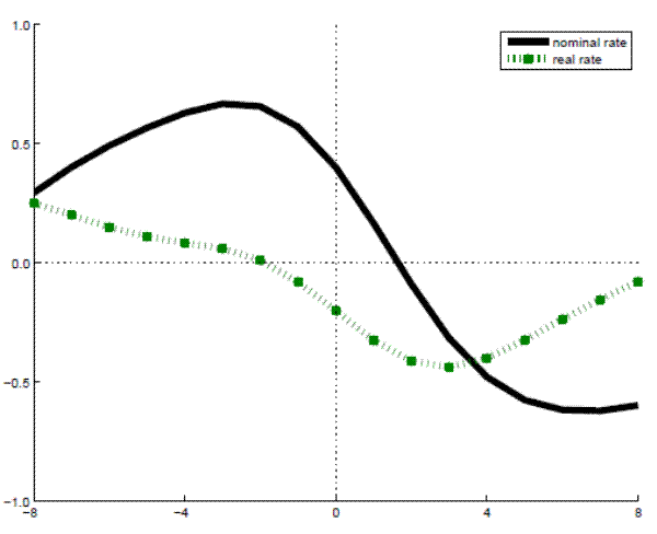
But in the data, the real rate is clearly counter-cyclical, it is negatively correlated with current output. As mentioned already, it is also a negative leading indicator. This commonly found pattern of correlation between bc-filtered output and short-term interest rates is depicted in Figure 1.3
Figure 1: Lead-lag Correlations for Output and Interest Rates
Note:
![]() where
where ![]() is bandpass-filtered per-capita
output and
is bandpass-filtered per-capita
output and ![]() is bandpass-filtered nominal, respectively real rate. This ex-ante real rate is constructed from the VAR described in Section 3 as
is bandpass-filtered nominal, respectively real rate. This ex-ante real rate is constructed from the VAR described in Section 3 as
![]() . Quarterly lags on the x-axis.U.S. data 1959-2006.
. Quarterly lags on the x-axis.U.S. data 1959-2006.
What is the correct conclusion from a mismatch between implications from a dynamic model and stylized facts? Modern dynamic models always involve a joint specification of fundamental economic structure and driving processes. Model outcomes, such as the output-interest rate correlation, involve the
compound effect of these two features. Yet, when "puzzling" findings are taken as evidence against a particular structural feature - such as sticky prices or portfolio adjustment costs - it is typically not acknowledged that the economy might alternatively be driven by different types of shocks
that yield different effects within the given structure. Yet, more carefully, it is simply unclear whether dynamic models fail (or succeed) because of their transmission mechanisms or because of the nature of their driving forces.
To shed more light on this important issue, I provide empirical evidence about output-interest rate comovement conditional on various types of shocks: Neutral technology shocks, monetary shocks, investment specific shocks and news about future productivity and permanent inflation shocks. The first two of these also drive the models of KingWatson:1996. The decomposition is applied both to a continuous sample of postwar data ranging from 1959-2006 as well as as to two sub-samples, commonly associated with the Great Inflation (1959-1979) and the Great Moderation (1982-2006)4, extending the original dataset of KingWatson:1996 by more than ten years.5 There are striking results of my decomposition, which are reported in Section 4 using plots analogous to Figure 1:
- After conditioning on neutral technology shocks, the real rate is pro-cyclical and a positive leading indicator - just the opposite of its unconditional behavior. In response to such permanent growth shocks, this is a common outcome for variants of the neoclassical growth model, be they of the RBC or the New Keynesian variety KingWatson:1996,Gali:NewPerspectives,walsh:tb2,Woodford:tb.
- Conditional on monetary shocks, the real rate is counter-cyclical and a negative leading indicator, which squares with simple New-Keynesian models, too.6
- A strong counter-cyclical, and negatively leading behavior of the real rate is attributed to news about future productivity; and to a lesser extent also to investment specific shocks.
- As in the full sample, the real rate has been counter-cyclical during the Great Inflation, mostly due to permanent inflation shocks. However, during the Great Moderation the real rate has been pro-cyclical, with technology shocks playing a more prominent role in accounting for its comovements with output.
Thus, for the full sample the "output-interest rate puzzle" is already defused by conditioning on two widely-studied shocks: Technology and monetary shocks, which counteract each other. Such opposing effects of shocks to "supply" and "demand" are a general theme in Keynesian models Benassy:1995. This result also carries over to the sub-sample analysis, which is motivated by growing evidence, documenting substantial changes in the behavior of macroeconomic data since the late 1970s and early 1980s.7 In particular, since the beginning of the 1980s--and at least until 2006--macroeconomic data has been characterized by a decrease in overall volatility, called the Great Moderation Bernanke:2004:GreatModeration, whereas the 1970s have been characterized by high and rising inflation rates, also known as the Great Inflation Sargent:1999:conquestbook,StockWatson:2007:inflationforecast.
Figure 2: Cyclical Behavior of Output and Interest Rates
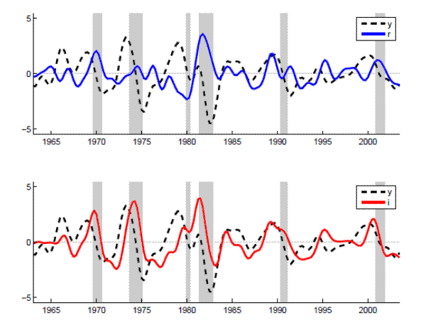
Note: Time series of bandpass-filtered output, nominal and real interest rates. The real rate is constructed from the VAR described in Section 3 as
![]() .
.
To foreshadow some of the sub-sample results, consider the time series of bandpass-filtered output and interest rates shown in Figure 2. As can be seen from the figure's upper panel, the counter-cyclicality of the real rate is most prevalent over the
Great Inflation, while it displays mostly positive comovements with output over the later part of the sample. The nominal rate behaves consistently pro-cyclical throughout the entire postwar period. What remains to be seen from the sub-sample decompositions presented in Section 4 is how these changes can mostly be attributed to changes in the relative importance of shocks, rather than substantial changes in the conditional comovements. This result is consistent with the study of SimsZha:2006:regimeswitching, who attribute changes in
macroeconomic dynamics over the postwar period mostly to changes in the amplitudes of shocks rather than changes in their transmission mechanism.
The backbone of my calculations is a VAR for the joint process of (unfiltered) output, nominal and real interest rate. The VAR serves both as a platform for identifying the structural shocks and to model the bc-filtered covariances and correlations. The identified shocks are shocks to the unfiltered data. For instance, both technology shocks have permanent effects on output but they might also have important effects on economic fluctuations. The point of bc-filtered statistics is to judge models solely on those cyclical properties, not on their implications for growth Prescott:1986. In this vein, the VAR is used to trace out the effects of shocks to the bc-filtered components of output and interest rates. This is done analytically using a frequency domain representation for the VAR and the bc-filters. Rotemberg:1996, Gali:1999 and denHaan:2000:comovements stress the importance of looking at conditional comovements in the context of the comovements of output with either prices or hours. In applying this general idea to output and interest rates, my specific approach is motivated by the fact that the "puzzle" in this area is typically expressed in terms of bc-filtered data.
The remainder of this paper is structured as follows: Related literature is briefly discussed in Section 2. Section 3 lays out my VAR framework for the identification of shocks as well as for decomposing the filtered covariances. Results are presented in Sections 4. Concluding comments are given in Section 5.
II Related Literature
To overcome the output-interest rate puzzle, BeaudryGuay:1996:realrates and BCF:2001 propose models with habit preferences and frictions to capital accumulation respectively sectoral factor immobility. This matches the real rate evidence by tweaking the transmission mechanism for a single kind of shock, namely technology. But the evidence presented in this study, suggests that the standard RBC mechanism for technology works fine.8FNbeaudryguay It is rather the interaction of several shocks leading to the "puzzling" evidence.9
In this spirit, RotembergWoodford:1997 report success with decision lags in a sticky price model10. The only structural shock they identify are disturbances to monetary policy. But their solution to the output-interest rate puzzle is based on the interaction with other shocks, which are left unidentified. This is revealed by their impulse response functions [Figure 1]RotembergWoodford:1997. Following a monetary shock, their model's output responses are negative (respectively zero) at all lags whilst they are positive for the nominal rate. Since conditional lead-lag covariances are just convoluted impulse responses, they are negative (respectively zero) at all leads and lags. This contrasts with the changing signs in the unconditional covariances depicted in my Figure 1 respectively their Figure 2.
Likewise, FuhrerMoore:1995 model the inverted leading indicator property of interest rates with multiple, non-structural shocks and couch their analysis just in terms of unconditional statistics. This paper is an empirical attempt to disentangle the underlying interaction of the various structural shocks.
III Empirical Methodology
The variables of interest for this paper are the logs of per-capita output11, the nominal as well as the real interest rate:
![]() . Let us call their bc-filtered component
. Let us call their bc-filtered component ![]() . The goal is to model and estimate how structural shocks induce comovements between the elements of
. The goal is to model and estimate how structural shocks induce comovements between the elements of ![]() .
.
The backbone of the calculations in this paper is a VAR. Since the real interest rate, ![]() is not fully observable, the VAR cannot be run directly over
is not fully observable, the VAR cannot be run directly over ![]() but rather over a vector of observables
but rather over a vector of observables ![]() . To sufficiently capture a wide-ranging set of structural shocks, the
logs of the following eleven variables are included in
. To sufficiently capture a wide-ranging set of structural shocks, the
logs of the following eleven variables are included in ![]() : the change in the relative price of investments, the growth rate in labor productivity, inflation, the ratios of consumption and
investment to output, hours worked, wage markups, capacity utilization, the nominal interest rate, the velocity of money and the spread between nominal long- and short-term interest rates:
: the change in the relative price of investments, the growth rate in labor productivity, inflation, the ratios of consumption and
investment to output, hours worked, wage markups, capacity utilization, the nominal interest rate, the velocity of money and the spread between nominal long- and short-term interest rates:
![]()
where ![]() . Apart from adding the long-term bond spread to the list of observables, this specification corresponds to the VAR used by ACEL. Details of the data construction are
described in Section 4. The dynamics of
. Apart from adding the long-term bond spread to the list of observables, this specification corresponds to the VAR used by ACEL. Details of the data construction are
described in Section 4. The dynamics of ![]() are captured by a
are captured by a ![]() -th order VAR:12
-th order VAR:12
The real rate is computed from the Fisher equation
![]() where inflation expectations are given by the VAR. So
where inflation expectations are given by the VAR. So ![]() can be constructed from
can be constructed from ![]() by applying a linear filter:
by applying a linear filter:
and where ![]() ,
, ![]() and
and ![]() are selection vectors such that
are selection vectors such that
![]() and so on.
and so on.
The remainder of this section describes the following: First, how the structural shocks are identified (Section 3.1). This gives us ![]() and the
conditional dynamics of the unfiltered variables can be computed from
and the
conditional dynamics of the unfiltered variables can be computed from
![]() . Second, how to apply a bc-filter to the structural components of
. Second, how to apply a bc-filter to the structural components of ![]() to obtain the decomposition of their auto-covariances (Section 3.2).
to obtain the decomposition of their auto-covariances (Section 3.2).
III.1 Identification of Structural Shocks
In order to identify a variety of structural shocks, which are commonly investigated by theoretical and empirical studies,13 this paper applies long-, medium- and short-run restrictions to the estimated VAR model. For the benchmark VAR, whose eleven variables are specified in (1), four structural shocks are identified: Investment-specific and neutral technology shocks, monetary policy shocks and news shocks about future productivity. When studying the sub-sample of the data associated with the Great Inflation (1959-1979), the VAR is respecified to allow for a common trend in inflation and nominal interest rates. For this model, innovations to this nominal trend are estimated as a fifth structural shock. Since all VAR models estimated here have more observables than identified shocks, there remains also an unidentified component, which is orthogonal to the identified shocks. These identification schemes are described below.
III.1.1 Investment-Specific and Neutral Technology Shocks
Two types of technology shocks are identified from long-run restrictions as it has been done before by Fisher:2006:invtech, ACEL, GaliGambetti:2008:aej. Investment-specific shocks are identified as the sole source of variations in the permanent component of the relative price of investments,
![]() . Neutral technology shocks are identified as driving the permanent component of labor-productivity (output per hour) beyond what is explained by the investment-specific technology
shocks.14 Since hours are assumed to be stationary, the identification scheme used here is actually equivalent to identifying (neutral) technology shocks
from the permanent component of output as in ShapiroWatson:1988.15
. Neutral technology shocks are identified as driving the permanent component of labor-productivity (output per hour) beyond what is explained by the investment-specific technology
shocks.14 Since hours are assumed to be stationary, the identification scheme used here is actually equivalent to identifying (neutral) technology shocks
from the permanent component of output as in ShapiroWatson:1988.15
The identifying restriction for both technology shocks imposes zero restrictions on ![]() :16
:16
The shocks are signed by imposing ![]() and
and ![]() ;
; ![]() is unrestricted.17 Together with the orthogonality of
the structural shocks, this identifies the first two column of
is unrestricted.17 Together with the orthogonality of
the structural shocks, this identifies the first two column of ![]() , which is then computed as in BlanchardQuah:1989.18 The standardized shocks to investment specific and neutral technology will be denoted
, which is then computed as in BlanchardQuah:1989.18 The standardized shocks to investment specific and neutral technology will be denoted
![]() and
and
![]() , respectively.
, respectively.
III.1.2 Monetary Policy Shocks
Shocks to monetary policy are defined as unexpected deviations from endogenous policy. As in CEE:HandbookMacro or RotembergWoodford:1997, the short-term interest rate is assumed to follow a linear policy rule
where
III.1.3 News Shocks about Future Productivity
News shocks have lately attracted considerable interest in theoretical and empirical work, with at least parts of the literature suggesting that they might play an important role in business cycle fluctuations BeaudryPortier:2006:news:aer,SchmittGroheUribe:news:nber,JaimovichRebelo:2009:news:aer. BarskySims:News and Sims:News identify news shock as "the shock orthogonal to technology innovations that best explains future variation in technology". While they use direct data on total factor productivity, their definition is applied here to labor productivity, as measured by the second element in the vector of VAR observables defined in (1). In addition to requiring that news have no contemporaneous impact on labor productivity, news shocks are assumed to be orthogonal to the other shocks identified in this study. Computational details of the identification strategy are described in Appendix B
III.1.4 Nominal Trend Shocks
When estimating the VAR over the "Great Inflation" sample (1959-1979), nominal trend shocks are identified as well. As described in Section 4.3 below, for this sub-sample the VAR is adapted to allow for a common trend in inflation and nominal
rates by replacing ![]() in (1) with
in (1) with ![]() and
and ![]() by
by ![]() . The nominal trend shocks are then
identified as the third element in the Blanchard-Quah factorization of the spectral density at frequency zero shown in (3).21 Such a trend could capture slow-moving fluctuations in policymakers' preferences for inflation--be these variations in their actual inflation target as in Ireland:2007:jmcb:InflationTarget or self-fullfiling market perceptions as in AlbanesiChariChristiano:2003 or
Sargent:1999:conquestbook.
. The nominal trend shocks are then
identified as the third element in the Blanchard-Quah factorization of the spectral density at frequency zero shown in (3).21 Such a trend could capture slow-moving fluctuations in policymakers' preferences for inflation--be these variations in their actual inflation target as in Ireland:2007:jmcb:InflationTarget or self-fullfiling market perceptions as in AlbanesiChariChristiano:2003 or
Sargent:1999:conquestbook.
III.2 Decomposition of BC-Filtered Covariances
Summarizing the previous discussion, the impulse responses of the unfiltered variables in ![]() are given by
are given by
![]() . These do not only trace out the business cycle responses of
. These do not only trace out the business cycle responses of ![]() to
the structural shocks
to
the structural shocks ![]() , but also how the shocks induce growth as well as high-frequency variations. The motivation for bc-filtering is to focus only on the business cycle
effects.22 Formally, it remains to apply a bc-filter and to decompose the filtered lead-lag covariances into the contributions of the structural shocks. The
computations are straightforward to perform in the frequency domain and a brief overview is given in A.
, but also how the shocks induce growth as well as high-frequency variations. The motivation for bc-filtering is to focus only on the business cycle
effects.22 Formally, it remains to apply a bc-filter and to decompose the filtered lead-lag covariances into the contributions of the structural shocks. The
computations are straightforward to perform in the frequency domain and a brief overview is given in A.
Since the bc-filtered variables in ![]() are covariance-stationary, their lead-lag covariances exist and so does their spectrum. They can be computed from the VAR parameters and the
filters
are covariance-stationary, their lead-lag covariances exist and so does their spectrum. They can be computed from the VAR parameters and the
filters ![]() and
and ![]() . To ease notation, the impulse responses of
. To ease notation, the impulse responses of ![]() after applying the bc-filter are written as
after applying the bc-filter are written as ![]() so that the bc-filtered spectrum can be expressed as
so that the bc-filtered spectrum can be expressed as
![]() . For each frequency
. For each frequency ![]() , this is simply a product of complex-numbered matrices. The lead-lag covariance matrices of
, this is simply a product of complex-numbered matrices. The lead-lag covariance matrices of ![]() can be recovered from the spectrum in what is known as an inverse
Fourier transformation
can be recovered from the spectrum in what is known as an inverse
Fourier transformation
![]()
Since the structural shocks are orthogonal to each other, the decomposition of the covariances
![]() is straightforward. First, the spectrum is computed conditional on each shock. Then, the conditional lead-lag covariances follow from an inverse Fourier transformation,
analogously to equation (4). To fix notation, the shocks are indexed by
is straightforward. First, the spectrum is computed conditional on each shock. Then, the conditional lead-lag covariances follow from an inverse Fourier transformation,
analogously to equation (4). To fix notation, the shocks are indexed by ![]() and
and ![]() is a square matrix, full of zeros except for a unit entry in its
is a square matrix, full of zeros except for a unit entry in its ![]() 'th diagonal element. The spectrum conditioned on shock
'th diagonal element. The spectrum conditioned on shock ![]() is
is
![]() . Since
. Since
![]() the conditional spectra add up to
the conditional spectra add up to
![]() . This carries over to the coefficients
. This carries over to the coefficients
![]() from the inverse Fourier transformation of
from the inverse Fourier transformation of
![]() such that
such that
![]() .
.
IV Decomposition Results
This section presents the results for the VAR described in the previous section. The VAR is estimated using quarterly data for the United States from 1959 to 2006. The construction of the data is described in C. The lag-length of each VAR used in this paper has been selected based on a comparison of information criteria, bootstrapped Portmanteau tests and the ability of the VAR to replicate bc-correlation computed from applying the Bandpass filter of BaxterKing:1999 directly to the data. Details can be found in the web-appendix for this paper, which has been attached at the end of this document.
To assess the statistical significance of the results, bootstrapped confidence intervals are computed for each shock. As discussed by SimsZha:1999:errorbands these are best interpreted as the posterior distributions from a Bayesian estimation with flat prior. The small sample adjustment of
Kilian:1998 is used to handle the strong persistence of the VAR23. In a first round, the small sample bias of the VAR coefficients is estimated from
![]() Monte Carlo draws. In the second round, the posterior distribution is constructed from
Monte Carlo draws. In the second round, the posterior distribution is constructed from ![]() draws using the VAR adjusted for the small sample bias.
draws using the VAR adjusted for the small sample bias.
The web-appendix documents the robustness of some of the key results reported below, when applying the decomposition to a much smaller, trivariate VAR, using only data on output, inflation and the nominal interest rate:
- Conditional on (neutral) technology, the real rate is pro-cyclical and a positive leading indicator.
- Technology shocks play a more substantial role over the Great Moderation, accounting for an unconditionally pro-cyclical real rate.
- The counter-cyclical, negatively leading behavior of the real rate during the Great Inflation is explained by permanent shocks to inflation.
IV.1 Full Sample
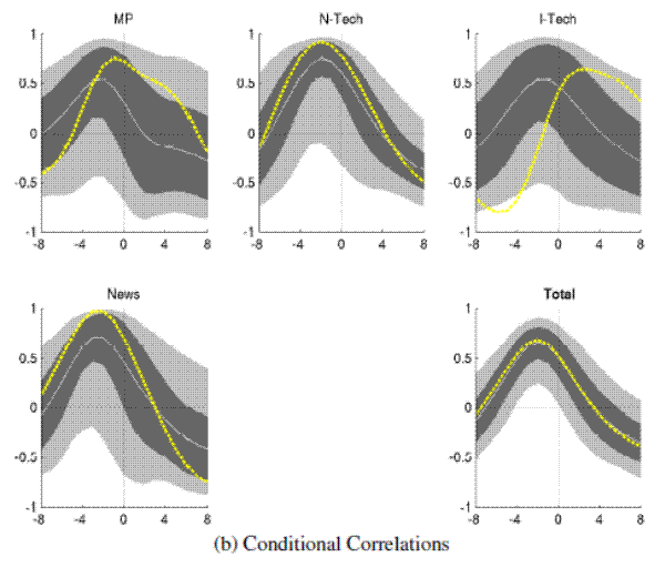
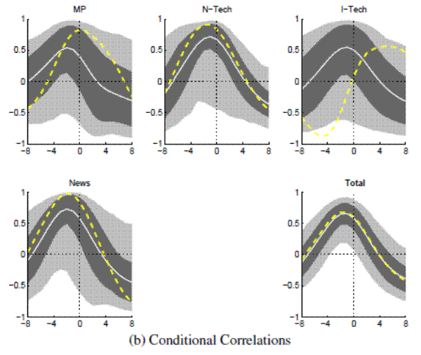
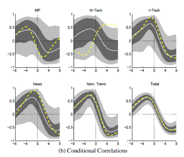
A result which consistently holds over the various samples considered here is that neutral technology shocks induce a strongly pro-cyclical real rate which is also a positive leading indicator for up to one year. For the full sample of data (1959-2006), this is depicted in the upper panel of Figure 3 which decomposes the filtered covariances between output and the real rate. Covariances add linearly, so they are a natural measure for the decomposition. The total covariances in Figure 3 are just a rescaling of the correlations reported in Figure 1 above. Figure 3 shows further that monetary shocks and news about future productivity induce negative covariances at leads between zero and up to two years. (To a much lesser, and largely insignificant extent, the same is true for investment specific technology shocks.) Turning to the nominal rate, all identified shocks contribute to its pro-cyclical and positively leading comovement with output. For brevity, these results are documented in a web-appendix, attached at the end of this document.
Figure 3A: Output and Real Rates: Conditional Comovements Covariance Decomposition
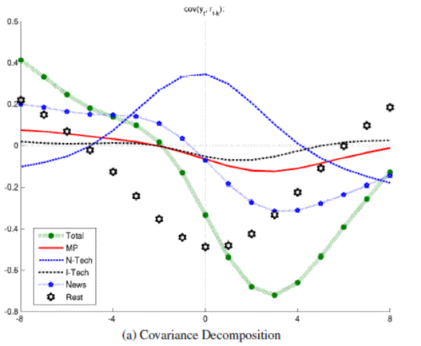
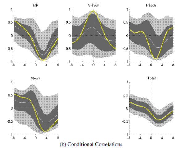
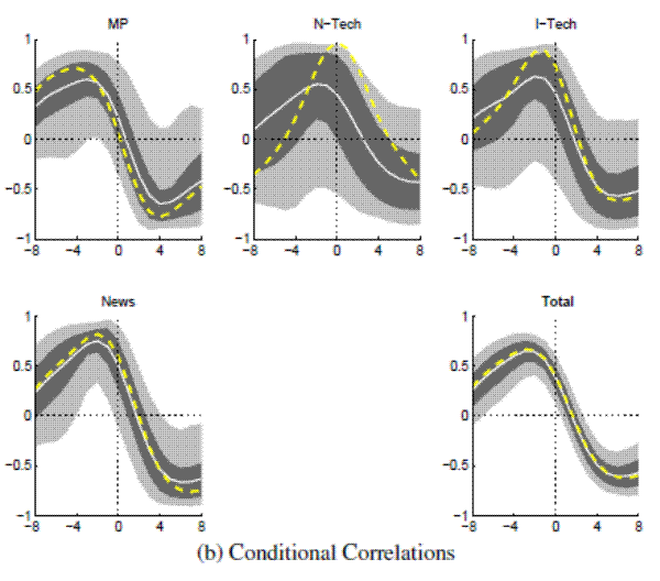
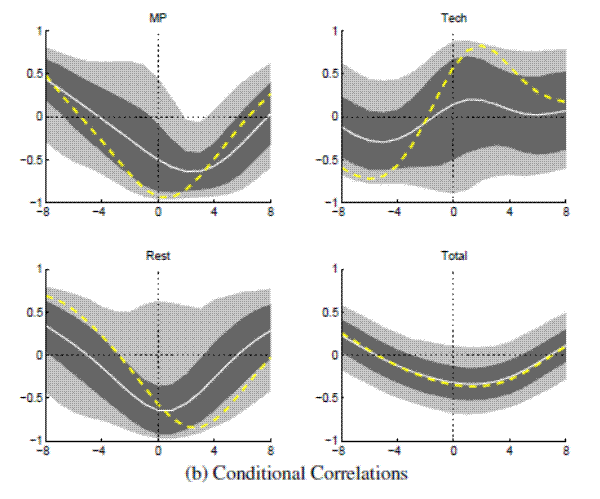
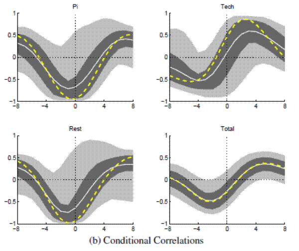
Figure 3B: Output and Real Rates: Conditional Comovements Conditional Correlations
 Note: Bandpass-filtered moments,
When adding up the conditional covariances induced by the four structural shocks, there remains an unidentified component, inducing a counter-cyclical real rate, comoving negatively with output at leads and lags of up to a year. Whilst monetary policy and news shocks help to account for the counter-cyclical, negatively leading real rate, their strength does at best offset the pro-cyclical and positively leading behavior induced by technology shocks. Still, the results clearly demonstrate that conditional comovements are far from being as puzzling as suggested by KingWatson:1996.
The comovements induced by monetary policy and news shocks are also significant as can be seen from the lower panel of Figure 3. There is much larger uncertainty and small sample bias associated with the technology shocks, reflecting that they are identified from the more uncertain, long run behavior of the data CEV:2006:macroannual. The small bias becomes apparent when comparing the point estimates of the VAR (dashed line) with the mean of the bootstrapped small sample distribution.24 When considering shape and location of the bootstrapped distributions the conditional correlations for neutral technology shocks, it is however reassuring that they are tilted towards pro-cyclical point estimates.
| Variables | Mon. Policy Shock | N-Tech Shock | I-Tech Shock | News Shock | Nom. Trend Shock | Rest Shock |
| Full Sample (1959-2006): Output | 6.36 | 15.09 | 7.29 | 26.70 | 44.56 | |
| Full Sample (1959-2006): Nom. rate | 11.24 | 11.04 | 3.72 | 43.91 | 30.09 | |
| Full Sample (1959-2006): Real rate | 9.92 | 31.43 | 3.27 | 17.71 | 37.67 | |
| Full Sample (1959-2006): Inflation | 4.30 | 2.60 | 13.24 | 29.06 | 50.80 | |
| Full Sample (1959-2006): Hours | 5.11 | 16.39 | 6.93 | 31.16 | 40.40 | |
| Great Moderation (1982-2006): Output | 0.88 | 56.50 | 5.39 | 15.23 | 22.00 | |
| Great Moderation (1982-2006): Nom. rate | 3.31 | 14.24 | 2.18 | 55.83 | 24.45 | |
| Great Moderation (1982-2006): Real rate | 3.54 | 16.85 | 6.84 | 43.56 | 29.21 | |
| Great Moderation (1982-2006): Inflation | 0.52 | 18.22 | 1.43 | 14.81 | 65.02 | |
| Great Moderation (1982-2006): Hours | 3.54 | 28.49 | 4.39 | 37.06 | 26.52 | |
| Great Inflation (1959-1979): Output | 3.74 | 5.57 | 12.41 | 18.16 | 30.59 | 29.53 |
| Great Inflation (1959-1979): Nom. rate | 7.49 | 5.63 | 6.28 | 14.67 | 39.32 | 26.60 |
| Great Inflation (1959-1979): Real rate | 11.76 | 4.25 | 22.75 | 6.84 | 28.06 | 26.33 |
| Great Inflation (1959-1979): Inflation | 3.71 | 4.83 | 15.82 | 14.36 | 36.20 | 25.08 |
| Great Inflation (1959-1979): Hours | 4.74 | 2.73 | 11.58 | 22.67 | 30.83 | 27.44 |
Note: Variance decomposition for bandpass-filtered variables computed from the VARs described in Sections 3 (Full Sample and Great Moderation) and 4.3 (Great Inflation). "Mon. Policy" is the monetary policy shock, "N-Tech" and "I-Tech" refer to the neutral, respectively investment specific technology shocks and "News" refers to the news shocks about future productivity whose identification is described in Section 3.1. As described in Section 4.3, the VAR estimated for the Great Inflation allows for a common trend in inflation and real rates. Shocks to this trend are labeled "Nom. Trend" above.
Since covariances can be negative as well as positive, it is ambiguous to put a number like "percentage explained" on their decomposition. Table 1 reports variance shares for the bandpass-filtered fluctuations induced by each shocks for output, inflation, interest rates and hours. For the full sample of postwar data, the identified shocks account for about half the business cycle fluctuations in output, inflation and hours and up to two-thirds of the variations in nominal and real interest rates -- mostly due to neutral technology shocks and news about future productivity. In the sub-sample analysis discussed below, the unexplained share of variations will mostly drop below a third of the total.
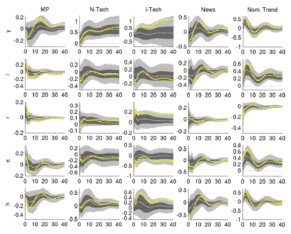
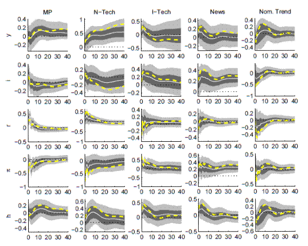
Figure 4: Impulse Responses
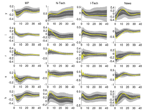 Note: Estimates for U.S. data (1959-2006) from VAR, equation (1) described in Section 3. Responses of unfiltered variables to a one-standard deviation shock (
So far the cyclical behavior of output and interest rates has been described in terms of bandpass-filtered covariances. Figure 4 documents the unfiltered impulse responses estimated for the full sample, and the results resonate very well with the filtered
comovements discussed above. Because of the non-trivial effects of bc-filtering25 it is however not a foregone conclusion, that the picture emerging from
the impulse responses should mirror the results for the bc-filtered comovements.
A monetary policy shocks increases the nominal rate for about a year, causing a prolonged contraction in output for up to four years as well as a reduction in inflation,26. In sum, the real rate rises while the economy contracts after a monetary shock. By construction, the neutral technology shock raises output permanently. As would be predicted by standard neoclassical growth models, e.g. such as the ones considered in KingWatson:1996, the technology induced growth in output is accompanied by an increase in the real rate for up to two years. Corroborating the results of Sims:News, output and hours drop in response to a news shock while the consumption output ratio increases.27 After an initial increase, the real rate drops as output recovers, in line with their counter-cyclical comovements documented for the business cycle frequencies in Figure 3. The full sample responses of real rate and output to investment specific shocks are largely insignificant.28
IV.2 Great Moderation
Reestimating the VAR described in Section 3 with data from the Great Moderation (1982-2006) yields considerably different results than what has been found above for the full sample of postwar data. However, just as in the full sample analysis, neutral technology shocks induce a pro-cyclical and positively leading real rate. Strikingly, the unconditional behavior of the real rate has been pro-cyclical and a positive leading indicator of output during the Great Moderation--just the opposite of what KingWatson:1996 have been puzzled about using data from 1959-1992.
Figure 5A: Output and Real Rates: Conditional Comovements (Great Moderation) Covariance Decomposition
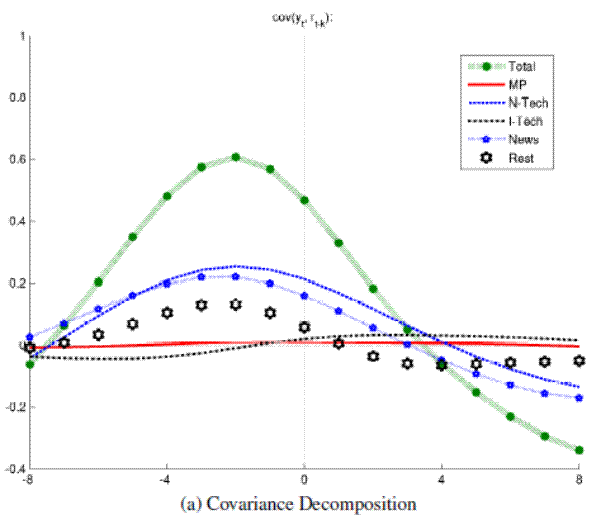
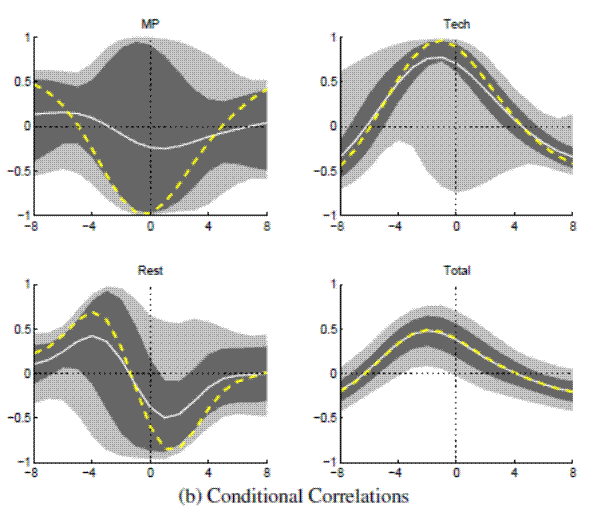
Figure 5B: Output and Real Rates: Conditional Comovements (Great Moderation) Conditional Correlations
 Note: Bandpass-filtered moments,
To a good extent the shift in the overall cyclicality of real rates can be attributed to an increase in the relative importance of neutral technology shocks as a source of business cycle fluctuations (see the middle panel of Table 1). Similarly, shocks to
investment specific technology and monetary policy induce a pro-cyclical real rate, however without being quantitatively relevant.
The second factor behind the change in the unconditional comovements is a different behavior in the responses to news shocks, which are estimated to induce a pro-cyclical real rate over the Great Moderation. Similar to the full sample results, the unfiltered impulse responses to news shocks still display a drop in aggregate activity while the real rate increases on impact before it drops shortly thereafter. However, in subsequent periods the movements in the real rate follow more closely the subsequent recovery in aggregate activity, compared to the more prolonged drop of the real rate after a news shock in the full sample estimates shown in Figure 4. (The impulse responses for the sub-samples are reported in a web-appendix attached at the end of this document.) These subtle changes in the unfiltered responses cause a significant shift in the cyclical components of real rate and output as witnessed by the decomposition results shown in Figure 5.
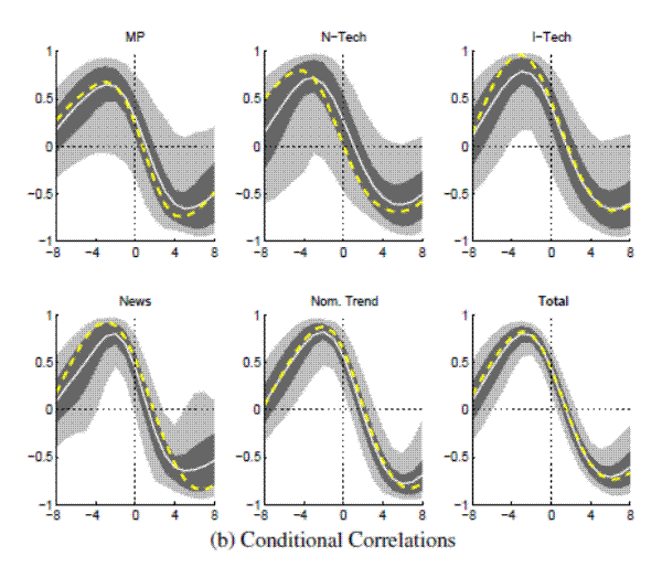
IV.3 Great Inflation
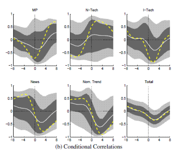
A notable feature of the Great Inflation (1959-1979) is the highly persistent rise in inflation, consistent with a common stochastic trend in inflation and nominal interest rates.29 Accordingly, the VAR specification described in Section 3 has been adapted to allow for such a common trend, by replacing the inflation rate with the change in inflation, and by replacing the nominal interest rate with the spread between the nominal interest rate and the contemporaneous inflation rate. This allows to identify permanent shocks to the common trend in inflation and nominal interest rates as described in Section 3.1.
In addition, the velocity of money, capacity utilization and wage markups have been dropped from the VAR, reflecting their very persistent behavior over this limited sample.30 The vector of VAR observables used for the Great Inflation sample is thus
![]()
Figure 6A: Output and Real Rates: Conditional Comovements (Great Inflation) Covariance Decomposition
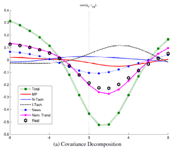
Figure 6B: Output and Real Rates: Conditional Comovements (Great Inflation) Covariance Correlations
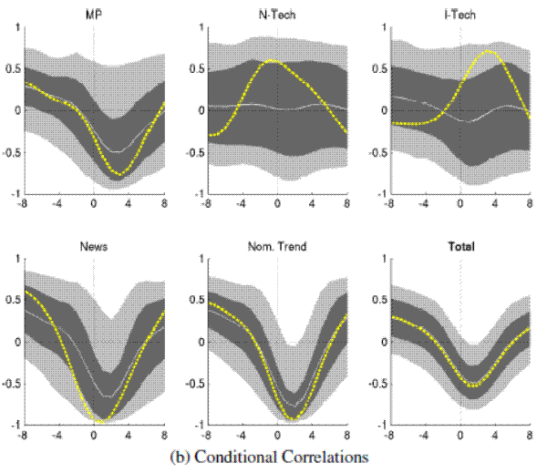
Note: Bandpass-filtered moments,
![]() , for U.S. data (1959-1979) computed from VAR allowing for a common trend in inflation and nominal rates as described in Section 4.3. Quarterly lags on the x-axis.Lower panel: Bootstrapped standard-errors bands with Kilian:1998's small sample adjustment (1000 draws in first round, 2000 draws in second). Percentiles are shaded: 95% (light) and 68% (dark). The sold line is the mean of the
bootstraps. The dashed line is the point estimate of the VAR.
, for U.S. data (1959-1979) computed from VAR allowing for a common trend in inflation and nominal rates as described in Section 4.3. Quarterly lags on the x-axis.Lower panel: Bootstrapped standard-errors bands with Kilian:1998's small sample adjustment (1000 draws in first round, 2000 draws in second). Percentiles are shaded: 95% (light) and 68% (dark). The sold line is the mean of the
bootstraps. The dashed line is the point estimate of the VAR.
What is new, is that a further part of the hitherto unexplained, counter-cyclical remainder of the real rate, can now be attributed to permanent inflation shocks. In response to a permanent increase in inflation, output rises temporarily whilst nominal rates do not sufficiently increase with inflation, causing a drop in real rates. These result are consistent with the (unfiltered) impulse responses found by Ireland:2007:jmcb:InflationTarget when estimating a New-Keynesian DSGE model with random walk shocks to an exogenous inflation target.31 The web-appendix reports similar decomposition results when allowing for a nominal trend over the entire sample of postwar data.
V Conclusions
An economic model specifies restrictions on how the economy responds to exogenous forces. Data may not conform to these predictions, either because the specified responses are wrong, or because the set of forces considered in the model does not sufficiently capture those impinging on the real world (or both).32 KingWatson:1996 report an output-interest rate puzzle, because of discrepancies in the unconditional correlations of output and interest rates in U.S. data and a variety of calibrated models. But it appears in a different light, once the bc-statistics are conditioned on structural shocks. At the root of the "puzzle" are not so much the transmission mechanisms of their models, but rather the interaction of several shocks and their relative importance in different sub-samples of the data. Three points stand out:
Conditional on technology shocks, the comovements between output and real rate lines up fairly well with standard models, be it the standard RBC model or the technology channel of textbook New-Keynesian models as studied by Gali:NewPerspectives, walsh:tb2 or Woodford:tb. For all specifications considered, the contemporaneous correlation between (bc-filtered) real rate and output is positive. Likewise, the real rate is a positive leading indicator of output for almost one year. Unconditionally, the real rate is widely reported to be just the opposite - namely counter- or a-cyclical and a negative leading indicator. Attempts to match this with technology shocks appear to be going in the wrong direction.33
The overall behavior of the real rate must be the outcome of an interaction of several shocks. Indeed: When conditioning on monetary shocks, the real rate is counter-cyclical and a negative leading indicator as predicted by the simple New-Keynesian models. In addition, news about future productivity contribute to the counter-cyclical behavior of the real rate over the postwar period. Such opposing responses to "supply" and "demand" shocks are a general theme in Keynesian models Benassy:1995.
The comovements between output and the real rate differ when comparing the Great Inflation (1959-1979) with the Great Moderation (1982-2006). As in the full sample, the real rate has been counter-cyclical during the Great Inflation, mostly due to permanent inflation shocks. However, during the Great Moderation the real rate has been pro-cyclical, with technology shocks playing a more prominent role in accounting for its comovements with output.
Acknowledgments
This paper is based on the first chapter of my dissertation at the University of Lausanne. I would like to thank the members of my thesis committee Jean-Pierre Danthine (chair), Philippe Bacchetta, Robert G. King and Peter Kugler, the editor, two anonymous referees as well as V.V. Chari, Jordi Gali, Jean Imbs, Jinill Kim, Andrew Levin, David Lopez-Salido and seminar participants at the Board of Governors, the Federal Reserve Bank of Minneapolis, the University of Lausanne and the Swiss National Bank for their many helpful comments and suggestions. All remaining errors are of course mine. The main part of this paper has been written while working at Study Center Gerzensee and I would like to thank the Center for its generous support during my dissertation. This research has been carried out within the National Center of Competence in Research "Financial Valuation and Risk Management" (NCCR FINRISK). NCCR FINRISK is a research program supported by the Swiss National Science Foundation. Earlier drafts of this paper have also been circulated under the title "Puzzling Comovements between Output and Interest Rates? Multiple Shocks are the Answer."
I Applying BC-Filters to VAR Model
Conceptually, the analysis in this paper is applicable to a wide class of bc-filters, including the HP-Filter, the approximate bandpass filter of BaxterKing:1999 as well as the exact bandpass filter. A classic reference for the necessary tools is Priestley:1981:spectral, and similar techniques
are employed by ACEL and CKM:BCA. For the computations it is key that the bc-filter can be written as a linear, two-sided, infinite horizon moving average whose coefficients sum to zero:34
![]() where
where
![]() and
and ![]() .
.
The bandpass-filter is a such a symmetric moving average. It is explicitly defined in the frequency domain and most of my calculations are carried out in the frequency domain. For frequencies
![]() , evaluate the filter at the complex number
, evaluate the filter at the complex number ![]() instead of the lag operator
instead of the lag operator ![]() . This is also known as the Fourier transform of the filter which represents it as a series of complex numbers (one for each frequency
. This is also known as the Fourier transform of the filter which represents it as a series of complex numbers (one for each frequency ![]() ). Requiring
). Requiring ![]() sets the zero-frequency component of the filtered time series to
zero. For instance, the bandpass filter passes only cycles between two and a half and eight years. For monthly data, it is specified as follows:
sets the zero-frequency component of the filtered time series to
zero. For instance, the bandpass filter passes only cycles between two and a half and eight years. For monthly data, it is specified as follows:
![\begin{align*} B(e^{-i\omega}) &= \begin{cases} 1 & \forall \, \vert\omega\vert \, \in \, \left[\frac{2 \pi}{8 \cdot 12},\frac{2 \pi}{2.5 \cdot 12}\right] \ 0 & \text{otherwise} \end{cases}\end{align*}](img96.gif)
This VAR framework is also capable of handling unit roots in ![]() . By construction,
. By construction, ![]() and thus
and thus ![]() has a unit root such that
has a unit root such that ![]() is infinite. When
computing the bc-filtered spectrum
is infinite. When
computing the bc-filtered spectrum
![]() ,
, ![]() takes precedence over this unit root. It is
straightforward to check that
takes precedence over this unit root. It is
straightforward to check that
![]() is well defined everywhere, except at frequency zero. So we can think of the nonstationary vector
is well defined everywhere, except at frequency zero. So we can think of the nonstationary vector ![]() as having a pseudo-spectrum
as having a pseudo-spectrum
![]() where
where
![]() and which exists for every frequency on the unit circle except zero.
and which exists for every frequency on the unit circle except zero.
II Identification of News Shocks
This section describes the identification of news shocks about future productivity. The identification strategy follows BarskySims:News and Sims:News who identify news shock as "the shock orthogonal to technology innovations that best explains future variation in technology". While they use direct data on total factor productivity, their definition is applied here to labor productivity, as measured by the second element in the VAR observables defined in (1). In addition to requiring that news have no contemporaneous impact on labor productivity, they are assumed to be orthogonal to the other shocks identified in this study (neutral and investment-specific technology shocks as well as monetary policy shocks.35 This orthogonality constraint can be easily accommodated by extending the method of Uhlig:2004:gnp as explained below.
For this method it is convenient to express the identification in terms of an orthonormal matrix ![]() and not in terms of the matrix of impact coefficients
and not in terms of the matrix of impact coefficients ![]() defined in equation (2) above. These two are related via the Cholesky decomposition of the VAR's forecast error variance,
defined in equation (2) above. These two are related via the Cholesky decomposition of the VAR's forecast error variance,
![]() :
:
![]() and
and
![]() . By construction we have
. By construction we have
![]() . We seek the column of
. We seek the column of ![]() , associated with the news
shock. Denoting this column as
, associated with the news
shock. Denoting this column as ![]() , it solves the following variance maximization problem
, it solves the following variance maximization problem
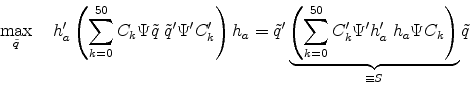
where
Uhlig:2004:gnp solves the above problem without the orthogonality constraint (6). In this case the problem reduces to finding the largest eigenvector of the positive definite matrix ![]() defined in (5) with
defined in (5) with ![]() being its normalized eigenvector.
being its normalized eigenvector.
A previous working paper version of this paper Mertens:szg:montblanc has extended Uhlig's computations to handle the orthogonality constraint (6) as follows:37 Let ![]() be an orthonormal basis for the nullspace of
be an orthonormal basis for the nullspace of
![]() . The set of permissible vectors
. The set of permissible vectors ![]() is then
is then
![]() where
where ![]() is the
dimension of the nullspace. Reparametrized in terms of
is the
dimension of the nullspace. Reparametrized in terms of ![]() , the problem reduces to set
, the problem reduces to set ![]() equal to the normalized eigenvector of of
equal to the normalized eigenvector of of ![]() associated with its largest eigenvalue, denoted
associated with its largest eigenvalue, denoted ![]() . The sign of
. The sign of ![]() (and thus the sign of the news shock) is determined by making it raise the consumption-output ratio on impact. It should be noted
that this sign restriction only affects the sign of first moments (e.g. impulse responses), but not the sign of second moments (e.g. conditional covariances), which are at the heart of this paper.
(and thus the sign of the news shock) is determined by making it raise the consumption-output ratio on impact. It should be noted
that this sign restriction only affects the sign of first moments (e.g. impulse responses), but not the sign of second moments (e.g. conditional covariances), which are at the heart of this paper.
III Data
The dataset used for this study has been collected from FRED38 and the Federal Reserve Board's G17 releases, which are publicly available. All data is quarterly and expressed in logs.39 Quantity variables have been converted to per-capita units using the Bureau Labor Statistics (BLS) measure of the civilian population over 16, interest rates and inflation rates have been annualized.
The data is largely identical to the time series used by ACEL for the sample 1959 to 2006. The only major difference is the use of NIPA data to construct the relative price of investments as in GaliGambetti:2008:aej and JustinianoPrimiceri:2008:TVP:aer, who construct the (log) relative price of investments as a weighted average of the (log) deflators of nondurables and services consumption minus the weighted average of the (log) deflators for investment and durable consumption, with the weights given by the relative (nominal) shares of each spending category,40 whereas ACEL use data constructed by Fisher:2006:invtech.
In detail, output (![]() ) is measured by real GDP per-capita and inflation is measured by the log-difference in the CPI index. As in ACEL, the (log-) ratios of consumption and investment to
output,
) is measured by real GDP per-capita and inflation is measured by the log-difference in the CPI index. As in ACEL, the (log-) ratios of consumption and investment to
output, ![]() and
and ![]() , are computed from nominal consumption and
investments as well as nominal GDP.41 Hours per capita,
, are computed from nominal consumption and
investments as well as nominal GDP.41 Hours per capita, ![]() are calculated from the BLS measure of nonfarm business hours. Wage markups,
are calculated from the BLS measure of nonfarm business hours. Wage markups,
![]() , are computed from the difference of nominal GDP less hours worked, less the BLS measure of nominal compensation per hour in the nonfarm business sector. Capacity
utilization,
, are computed from the difference of nominal GDP less hours worked, less the BLS measure of nominal compensation per hour in the nonfarm business sector. Capacity
utilization, ![]() , is measured for the manufacturing industry as reported by the Federal Reserve Board's G17 release.42 The quarterly average of nominal yields on three month Treasury Bills is used for the nominal short-term interest rate,
, is measured for the manufacturing industry as reported by the Federal Reserve Board's G17 release.42 The quarterly average of nominal yields on three month Treasury Bills is used for the nominal short-term interest rate, ![]() . The term spread of nominal interest rates is computed from the short-term interest rate and the 10-year Treasury constant maturity rate. The velocity of money,
. The term spread of nominal interest rates is computed from the short-term interest rate and the 10-year Treasury constant maturity rate. The velocity of money,
![]() , is computed from the log-difference between nominal GDP and the money-at-zero-maturity measure computed by the Federal Reserve Bank of St. Louis.
, is computed from the log-difference between nominal GDP and the money-at-zero-maturity measure computed by the Federal Reserve Bank of St. Louis.
Part : Web-Appendix
This is the web-appendix with supplementary details of the VAR lag-length selection (Section I), additional results for the large VARs, which are also used in the main paper (Section II) as well as results for smaller, trivariate VARs, which use only data on output, inflation and the nominal short-term interest rate (Section III).
I Lag-Length Selection
Specification of the VAR's lag-length is based on a comparison of information criteria, bootstrapped Portmanteau tests and the ability of the VAR to replicate bc-correlation computed from applying the Bandpass filter of BaxterKing:1999 directly to the data.43 Lag-Length selection tables and plots of the autocovariance functions for the VARs used in the main paper are presented below.
| VAR: lag | VAR: T-K | VAR: llf/T | VAR: max root | Information Criteria: AIC | Information Criteria: HQIC | Information Criteria: SIC | Portmanteau Tests for lags: 4 | Portmanteau Tests for lags: 8 | Portmanteau Tests for lags: 10 | Portmanteau Tests for lags: 12 | Portmanteau Tests for lags: 16 | Portmanteau Tests for lags: 18 | Portmanteau Tests for lags: 20 |
| 1 | 178 | -11.05 | 0.9881 | 23.49 | 24.41 | 25.75 |
688.21** | 1297.69** | 1580.05** | 1867.45** | 2387.65** | 2659.14** | 2916.48** |
| 2 | 166 | -10.25 | 0.9899 | 23.19 | 24.94 | 27.53 | 458.73** | 1024.55** | 1303.42** | 1590.83** | 2092.52** | 2357.49** | 2607.01** |
| 3 | 154 | -9.48 | 0.9905 | 22.93 | 25.54 | 29.37 | 281.81 | 830.16** | 1092.80** | 1374.52** | 1863.32** | 2133.33** | 2374.64** |
| 4 | 142 | -8.87 | 0.9918 | 23.03 | 26.50 | 31.59 | 207.07 | 721.60 | 988.32 |
1254.53 |
1745.60 |
2009.33 |
2261.62 |
| 5 | 130 | -8.24 | 0.9977 | 23.11 | 27.44 | 33.79 | 165.41 | 651.57 | 928.10 | 1200.37 | 1715.08 |
1977.33 |
2238.14 |
| 6 | 118 | -7.55 | 1.0055 | 23.06 | 28.26 | 35.89 | 177.79 | 600.30 | 874.35 | 1157.61 | 1680.78 | 1948.61 | 2209.05 |
| 7 | 106 | -6.90 | 1.0022 | 23.12 | 29.20 | 38.12 | 194.70 | 571.37 | 856.21 | 1119.12 | 1620.36 | 1874.85 | 2124.78 |
| 8 | 94 | -6.16 | 0.9940 | 23.02 | 29.98 | 40.19 | 241.23 | 610.63 | 914.81 | 1179.07 | 1676.77 | 1915.52 | 2146.17 |
| 9 | 82 | -5.21 | 1.0031 | 22.50 | 30.35 | 41.86 | 299.36 | 635.32 | 870.95 | 1140.96 | 1649.86 | 1896.51 | 2136.42 |
| 10 | 70 | -3.97 | 0.9993 | 21.43 | 30.18 | 43.01 | 394.48 | 828.13 | 1032.45 | 1316.03 | 1802.79 | 2064.12 | 2307.86 |
| 12 | 46 | -1.08 | 1.0030 | 18.51 |
29.07 | 44.56 | 591.20 | 1122.76 | 1375.56 | 1631.89 | 2125.80 | 2390.27 | 2624.10 |
Note: Model chosen with lag-length 3.
Figure A.7: BC-Moments: Filtered VAR versus Data (Large VAR, Full Sample)
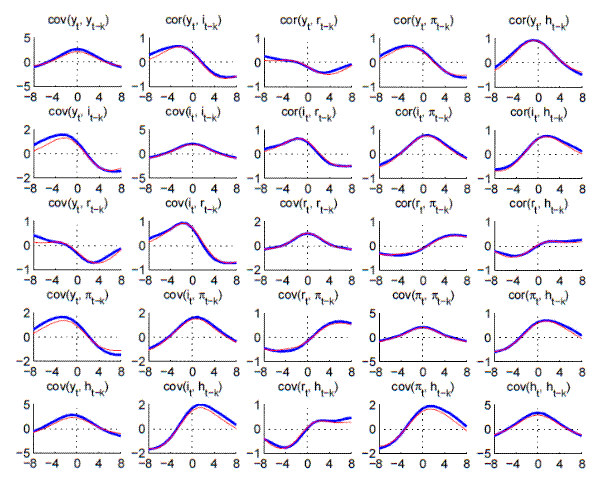 Note: Bandpass-filtered moments,
| VAR: lag | VAR: T-K | VAR: llf/T | VAR: max root | Information Criteria: AIC | Information Criteria: HQIC | Information Criteria: SIC | Portmanteau Tests for lags: 4 | Portmanteau Tests for lags: 8 | Portmanteau Tests for lags: 10 | Portmanteau Tests for lags: 12 | Portmanteau Tests for lags: 16 | Portmanteau Tests for lags: 18 | Portmanteau Tests for lags: 20 |
|
1 |
84 | -7.58 | 0.9854 | 17.92 | 19.34 |
21.44 |
552.92** | 1074.39 |
1306.45 | 1573.62 | 2029.30 | 2260.28 | 2471.24 |
| 2 | 72 | -5.68 | 0.9787 | 16.68 | 19.43 | 23.48 | 427.30 | 933.69 | 1174.00 | 1464.41 | 1915.26 | 2126.01 | 2360.92 |
| 3 | 60 | -4.07 | 1.0218 | 16.10 | 20.18 | 26.22 | 361.85 | 892.27 | 1140.30 | 1432.11 | 1945.63 | 2200.74 | 2468.93 |
| 4 | 48 | -2.74 | 0.9788 | 16.12 | 21.56 | 29.60 | 348.57 | 851.17 | 1140.38 | 1431.08 | 1927.28 | 2176.18 | 2455.66 |
| 5 | 36 | -0.17 | 0.9989 | 13.72 | 20.54 | 30.61 | 428.87 | 960.38 | 1281.58 | 1593.88 | 2148.05 | 2422.73 | 2723.53 |
| 6 | 24 | 2.43 | 1.0126 | 11.33 |
19.53 | 31.66 | 634.86 | 1142.21 | 1417.21 | 1698.30 | 2253.84 | 2553.62 | 2845.22 |
Note: Model chosen with lag-length 2. ![]() denotes minimum IC. Q-statistics for Portmanteau test.
denotes minimum IC. Q-statistics for Portmanteau test. ![]() denotes significance at the 10%,
denotes significance at the 10%, ![]() at the 5%,
at the 5%, ![]() at the 1% level of bootstrapped distribution (2000 draws). The column labeled
at the 1% level of bootstrapped distribution (2000 draws). The column labeled ![]() reports the degrees of freedom in each estimation, measured by the number of
observations after dropping initial values (
reports the degrees of freedom in each estimation, measured by the number of
observations after dropping initial values (![]() ) less the number of VAR coefficients to be estimated (
) less the number of VAR coefficients to be estimated (![]() ).
). ![]() reports the log-likelihood of each VAR scaled by the number of observations. AIC, HQIC and SIC denote the Akaike Information Criteria, Hannan-Quinn and
Schwarz Information Criteria, respectively.
reports the log-likelihood of each VAR scaled by the number of observations. AIC, HQIC and SIC denote the Akaike Information Criteria, Hannan-Quinn and
Schwarz Information Criteria, respectively.
Figure A.8: BC-Moments: Filtered VAR versus Data (Large VAR, Great Moderation)
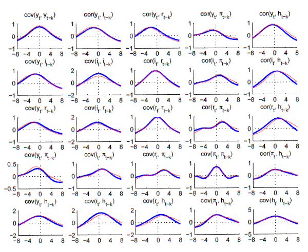 Note: Bandpass-filtered moments,
| VAR: lag | VAR: T-K | VAR: llf/T | VAR: max root | Information Criteria: AIC | Information Criteria: HQIC | Information Criteria: SIC | Portmanteau Tests for lags: 4 | Portmanteau Tests for lags: 8 | Portmanteau Tests for lags: 10 | Portmanteau Tests for lags: 12 | Portmanteau Tests for lags: 16 | Portmanteau Tests for lags: 18 | Portmanteau Tests for lags: 20 |
| 1 | 71 | -6.85 | 0.9847 | 15.51 | 16.37 |
17.65 |
271.51 |
538.25 |
654.48 | 796.43 | 1112.04 |
1254.15 |
1385.88 |
| 2 | 62 | -6.08 | 0.9918 | 15.60 | 17.23 | 19.68 | 197.50 | 477.95 | 603.71 | 733.81 | 1012.81 | 1155.47 | 1285.33 |
| 3 | 53 | -5.13 | 0.9869 | 15.39 | 17.80 | 21.43 | 148.08 | 428.01 | 551.13 | 677.43 | 944.63 | 1075.99 | 1204.03 |
| 4 | 44 | -4.27 | 0.9767 | 15.40 | 18.61 | 23.44 | 136.64 | 413.19 | 538.61 | 669.48 | 941.23 | 1076.62 | 1205.73 |
| 5 | 35 | -2.99 | 0.9981 | 14.60 | 18.62 | 24.66 | 146.57 | 423.39 | 555.64 | 691.19 | 970.83 | 1127.91 | 1288.69 |
| 6 | 26 | -1.41 | 1.0138 | 13.28 |
18.12 | 25.39 | 250.10 | 533.02 | 649.68 | 804.84 | 1097.23 | 1248.38 | 1414.31 |
Figure A.9: BC-Moments: Filtered VAR versus Data (Large VAR, Great Inflation)
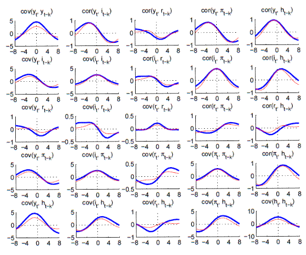 Note: Bandpass-filtered moments,
II Additional Results for Large VARs
This section reports the following results:
- Impulse Responses estimated for the Great Moderation and the Great Inflation
- Decompositions for comovements between output and the nominal rate
- Results obtained from estimating a VAR allowing for a common stochastic trend in inflation and nominal rates over the full sample of postwar data. In addition to what is described in Section 4.3 of the main paper, the VAR includes also the velocity of money as well as the ratio of total reserves to the price level.
Figure A.10: Impulse Responses (Large VAR, Great Moderation)
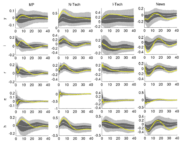 Note: Estimates for U.S. data (1982-2006) from VAR, equation (1) in Section 3 of the main paper. Responses of unfiltered variables to a one-standard deviation shock (
Figure A.11: Impulse Responses (Large VAR, Great Inflation)
 Note: Estimates for U.S. data (1959-1979) from VAR with nominal trend, described in Section 4.3 of the main paper. Responses of unfiltered variables to a one-standard deviation shock (
Figure A.12A: Output and Nominal Rates (Large VAR, Full Sample) Covariance Decomposition
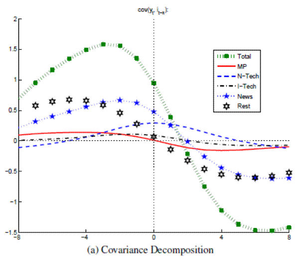
Figure A.12B: Output and Nominal Rates (Large VAR, Full Sample) Conditional Correlations
 Note: Bandpass-filtered moments,
Figure A.13A: Output and Nominal Rates (Large VAR, Great Moderation) Covariance Decomposition
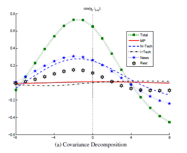
Figure A.13B: Output and Nominal Rates (Large VAR, Great Moderation) Conditional Correlations
 Note: Bandpass-filtered moments,
Figure A.14A: Output and Nominal Rates (Large VAR, Great Inflation) Covariance Decomposition
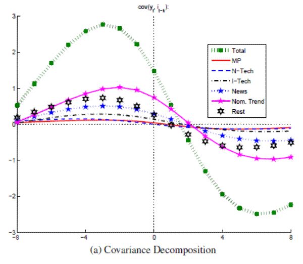
Figure A.14B: Output and Nominal Rates (Large VAR, Great Inflation) Conditional Correlations
 Note: Bandpass-filtered moments,
Figure A.15: Impulse Responses (Full Sample w/Nominal Trend)
 Note: Estimates for U.S. data (1959-1979) from VAR with nominal trend. Responses of unfiltered variables to a one-standard deviation shock (
Figure A.16A: Output and Real Rates (Full Sample w/Nominal Trend) Covariance Decomposition
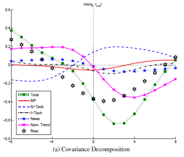
Figure A.16B: Output and Real Rates (Full Sample w/Nominal Trend) Conditional Correlations
 Note: Bandpass-filtered moments,
Figure A.17A: Output and Nominal Rates (Full Sample w/Nominal Trend) Covariance Decomposition
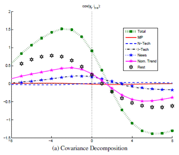
Figure A.17B: Output and Nominal Rates (Full Sample w/Nominal Trend) Conditional Correlations
 Note: Bandpass-filtered moments,
III Results for Small VARs
As a robustness check, this appendix reports decomposition results obtained from smaller, trivariate VARs, using the bare minimum of variables, which are needed to model output and the real interest rate: output growth, inflation and the nominal interest rate. As in the main paper, a common trend in inflation and nominal rate is allowed for when estimating the VAR for the Great Inflation. The trivariate VAR cannot be used to identify as many shocks as with the larger VAR used in the main paper. Attention is limited here to the identification of neutral technology shocks, as being the sole driver of the permanent component in output, as well as nominal trend shocks (when estimating the VAR for the Great Inflation). Confirming results from the main paper, the key findings from this exercise are that the real rate is pro-cyclical when conditioned on technology shocks, and counter-cyclical when conditioned on nominal trend shocks during the Great Inflation.
In the main paper, the permanent component of labor productivity is driven by neutral and investment-specific technology shocks. Since hours are assumed to be stationary, the permanent component of labor productivity is identical to the permanent component of output and the technology shocks identified here correspond to a mixture of both types of technology shocks identified in the main paper. In all three samples considered (Full, Great Moderation and Great Inflation), the real rate is pro-cyclical when conditioned on technology shocks.
For the VAR specification with stationary inflation, results are also reported for "Monetary Policy" which are simply identified by projecting the innovation of the nominal rate off the technology shocks and the innovation in inflation, which is unlikely to properly account for endogenous policy responses to variations in aggregate activity and inflation. Still, the results mirror the conditionally counter-cyclical behavior of the real rate reported in the main paper for the larger VARs.
Figure A.18A: Output and Real Rate decomposed with Small VAR (Full Sample) Covariance Decomposition
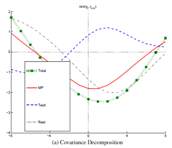
Figure A.18B: Output and Real Rate decomposed with Small VAR (Full Sample) Conditional Correlations
 Note: Bandpass-filtered moments,
Figure A.19A: Output and Real Rate decomposed with Small VAR (Great Moderation) Covariance Decomposition
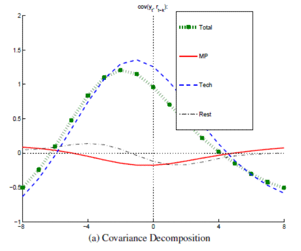
Figure A.19B: Output and Real Rate decomposed with Small VAR (Great Moderation) Conditional Correlations
 Note: Bandpass-filtered moments,
Figure A.20A: Output and Real Rate decomposed with Small VAR (Great Inflation) Covariance Decomposition
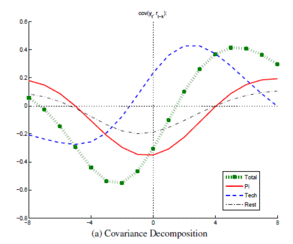
Figure A.20B: Output and Real Rate decomposed with Small VAR (Great Inflation) Conditional Correlations
 Note: Bandpass-filtered moments,