Skip to: [Printable Version (PDF)] [Bibliography] [Footnotes]

Finance and Economics Discussion Series: 2010-29 Screen Reader version ^♣

Documentation of the Estimated, Dynamic, Optimization-based (EDO) Model of the U.S. Economy: 2010 Version

Hess Chung, Michael T. Kiley, and Jean-Philippe Laforte *

Keywords: DSGE model, policy model

Abstract:

This paper provides documentation for a large-scale estimated DSGE model of the U.S. economy - the Federal Reserve Board's Estimated, Dynamic, Optimization-based (FRB/EDO) model project. The model can be used to address a wide range of practical policy questions on a routine basis. The paper discusses the model's specification, estimated parameters, and key properties.

This paper contains documentation for the large-scale estimated DSGE model of the U.S. economy currently used at the Federal Reserve Board for some forecasting and policy projects - the Estimated, Dynamic, Optimization-based (EDO) model. Section 1 provides a brief qualitative description of the model and outlines its main features for production, capital evolution, and preference technologies. Section 2 defines the equilibrium of the model. Section 3 lists the data that is used in estimating the model. Section 4 reports the model's key estimation results, which include the estimated parameter values, variance decompositions, impulse response functions, and estimated paths of the exogenous processes driving the model. The equations that characterize equilibrium in this model are contained in the appendix. Appendix A reports the equations of the symmetric and stationary model, and appendix B gives the solution to the model's steady-state. Finally, since the model contains a large number of parameter and variable names a key is given in appendices C, D, and E.

Before moving to our presentation of the model, we note that the EDO model serves as a complement to the analyses that are currently performed using existing large-scale econometric models, such as FRB/US model, as well as smaller, ad hoc models that we have found useful for more specific questions. In our experience, model-based analyses are enhanced by consideration of multiple models (and, indeed, our experience suggests that often we learn as much when models disagree than when they agree). A benefit of having multiple models is the opportunity to examine the robustness of policy strategies across models with quite different foundations, which we view as important given the significant divergences of opinion regarding the plausibility of various types of models.

In addition, the EDO model is designed to allow the straightforward consideration of factors not explicitly modeled in the baseline version of the model. For example, the baseline version assumes that investment decisions - of households and firms - are made by capital intermediaries; simple modifications of this intermediation step allow explicit consideration of the financial accelerator or financial intermediation (e.g., a banking sector), topics of ongoing research.

These advantages of the model have been demonstrated in previous research on its forecast performance (Edge, Kiley, and Laforte (2010)), its application to policy questions such as the natural rate (Edge, Kiley, and Laforte (2008)), and the analysis of the cyclical state of the economy (Kiley (2010b)).

1 Model Overview and Motivation

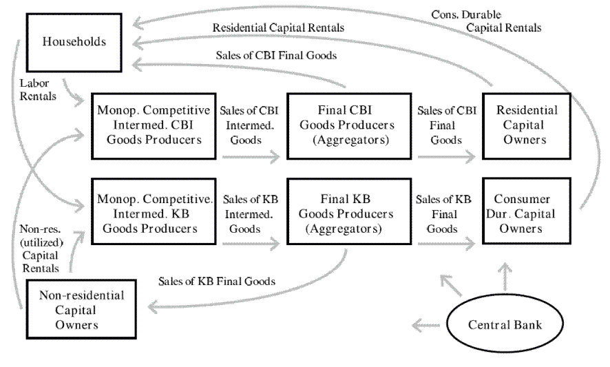
Figure 1 provides a graphical overview of the model.

The model possesses two final good sectors in order to capture key long-run growth facts and to differentiate between the cyclical properties of different categories of durable expenditure (e.g., housing, consumer durables, and nonresidential investment). For example, technological progress has been faster in the production of business capital and consumer durables (such as computers and electronics). Edge, Kiley, and Laforte (2008 and 2010) discuss this motivation in greater detail. The first sector is the slow-growing sector--called "CBI" because most of these goods are used for consumption (C) and because they are produced by the business and institutions (BI) sector--and the second is the fast-growing sector--called "KB" because these goods are used for capital (K) accumulation and are produced by the business (B) sector. The goods are produced in two stages by intermediate- and then final-goods producing firms (shown in the center of the figure). As in most new-Keynesian models, the introduction of intermediate and final goods producers facilitates the specification of nominal rigidities.

The disaggregation of production (aggregate supply) leads naturally to some disaggregation of expenditures (aggregate demand). We move beyond the typical model with just two categories of (private domestic) demand (consumption and investment) and distinguish between four categories of private demand: consumer non-durable goods and non-housing services, consumer durable goods, residential investment, and non-residential investment. The boxes surrounding the producers in the figure illustrate how we structure the sources of each demand category. Consumer non-durable goods and services are sold directly to households; consumer durable goods, residential capital goods, and non-residential capital goods are intermediated through capital-goods intermediaries (owned by the households), who then rent these capital stocks to households. Consumer non-durable goods and services and residential capital goods are purchased (by households and residential capital goods owners, respectively) from the first of economy's two final goods producing sectors, while consumer durable goods and non-residential capital goods are purchased (by consumer durable and residential capital goods owners, respectively) from the second sector. In addition to consuming the non-durable goods and services that they purchase, households supply labor to the intermediate goods-producing firms in both sectors of the economy.

This remainder of this section provides an overview of the decisions made by each of the agents in our economy. Given some of the broad similarities between our model and others, our presentation is selective.

1.1 The Final Goods Producers' Problem

The economy produces two final goods and services: slow-growing "consumption" goods and services, $X^{cbi}_{t}$ , and fast-growing "capital" goods, $X^{kb}_{t}$ . These final goods are produced by aggregating (according to a Dixit-Stiglitz technology) an infinite number of sector-specific differentiated intermediate inputs, $X_{t}^{s}(j)$ for , distributed over the unit interval. The representative firm in each of the consumption and capital goods producing sectors chooses the optimal level of each intermediate input, taking as given the prices for each of the differentiated intermediate inputs, $P_{t}^{s}(j)$ , to solve the cost-minimization problem:

$\displaystyle \min_{\left\{ X_{t}^{s}(j)\right\} _{j=0}^{1}} \int_{0}^{1}P_{t}^{s}(j)X_{t}^{s}(j)dj\mathrm{\ subject \ to \ } \left( \int_{0}^{1}\left(X_{t}^{s}(j)\right)^{\frac{\Theta^{s}_{t}-1} {% \Theta^{s}_{t}}}dj\right)^{\frac{\Theta^{s}_{t} } {\Theta^{s}_{t}-1}} \geq X^{s}_{t},\ \mathrm{for} \ s=cbi,kb.$

(1)

The term $\Theta^{s}_{t}$ is the stochastic elasticity of substitution between the differentiated intermediate goods inputs used in the production of the consumption or capital goods sectors. Letting $\theta^{s}_{t} \equiv \ln \Theta^{s}_{t}-\ln \Theta^{s}_{\ast}$ denote the log-deviation of $% \Theta^{s}_{t}$ from its steady-state value of $\Theta^{s}_{\ast}$ , we assume that

$\displaystyle \theta_{t}^{s}=\epsilon_{t}^{\theta,s},\ \mathrm{for} \ s=cbi,kb,$

(2)

where $\epsilon_{t}^{\theta,s}$ is a shock process. A stochastic elasticity of substitution introduces transitory markup shocks into the pricing decisions of intermediate-goods producers.

1.2 The Intermediate Goods Producers' Problem

The intermediate goods entering each final goods technology are produced by aggregating (according to a Dixit-Stiglitz technology) an infinite number of differentiated labor inputs, $L_{t}^{s}(j)$ for , distributed over the unit interval and combining this aggregate labor input (via a Cobb-Douglas production function) with utilized non-residential capital, $% K_{t}^{u,nr,s}$ . Each intermediate-good producing firm effectively solves three problems: two factor-input cost-minimization problems (over differentiated labor inputs and the aggregate labor and capital) and one price-setting profit-maximization problem.

In its first cost-minimization problem, an intermediate goods producing firm chooses the optimal level of each type of differential labor input, taking as given the wages for each of the differentiated types of labor, $% W_{t}^{s}(i)$ , to solve:

$\displaystyle \min_{\left\{ L^{s}_{t}(i,j)\right\} _{i=0}^{1}} \int_{0}^{1} W_{t}^{s}(i)L^{s}_{t}(i,j)di\mathrm{\ subject \ to \ } \left(\int_{0}^{1}\left(L^{s}_{t}(i,j)\right)^{\frac{\Theta^{l}_{t}-1} {% \Theta_{t}^{l}}} di\right)^{\frac{\Theta^{l}_{t}} {\Theta^{l}_{t}-1}} \geq L^{s}_{t}(j),\ \mathrm{for} \ s=cbi,kb.$

(3)

The term $\Theta^{l}_{t}$ is the stochastic elasticity of substitution between the differentiated labor inputs. Letting $\theta^{l}_{t} \equiv \ln \Theta^{l}_{t}-\ln \Theta^{l}_{\ast}$ denote the log-deviation of $% \Theta^{l}_{t}$ from its steady-state value of $\Theta^{l}_{\ast}$ , we assume that

$\displaystyle \theta_{t}^{l}=\epsilon_{t}^{\theta,l}.$

(4)

where $\epsilon_{t}^{\theta,l}$ is a shock process. A stochastic elasticity of substitution introduces transitory wage markup shocks into the wage decisions of households.

In its second cost-minimization problem, an intermediate-goods producing firm chooses the optimal levels of aggregated labor input and utilized capital, taking as given the wage, $W_{t}^{s}$ , for aggregated labor, $% L_{t}^{s}$ (which is generated by the cost function derived the previous problem), and the rental rate, $R^{nr,s}_{t}$ , on utilized capital, $% K^{u,nr,s}_{t}$ , to solve:

		$\displaystyle \min _{\left\{ L^{s}_{t}(j),K^{u,nr,s}_{t}(j)\right\} } W^{s}_{t}L^{s}_{t}(j)+R^{nr,s}_{t}K^{u,nr,s}_{t}(j)$
		$\displaystyle \mathrm{\;subject\;to \;} \left(Z^{m}_{t}Z^{s}_{t}L^{s}_{t}(j)\right)^{1-\alpha} \left(K^{u,nr,s}_{t}(j)\right)^{\alpha}\geq X^{s}_{t}(j),\;\mathrm{for}% \;s=cbi,kb, \;\mathrm{with}\;Z^{cbi}_{t}\equiv 1. \ \ \ \$	(5)

The parameter $\alpha$ is the elasticity of output with respect to capital, while the $Z_{t}$ variables denote the level of productivity. The level of productivity has two components. The first, $Z^{m}_{t}$ , is common to both sectors and thus represents the level of economy-wide technology. The second, $Z^{s}_{t}$ , is sector specific; we normalize $Z^{cbi}_{t}$ to one, while $Z^{kb}_{t}$ is not restricted.

The exogenous productivity terms contain a unit root, that is, they exhibit permanent movements in their levels. We assume that the stochastic processes $Z^{m}_{t}$ and $Z^{kb}_{t}$ evolve according to

$\displaystyle \ln Z^{n}_{t} - \ln Z^{n}_{t-1} =\ln \Gamma^{z,n}_{t} =\ln \left(\Gamma^{z,n}_{\ast} \cdot \exp[\epsilon^{z,n}_{t}] \right) =\ln \Gamma^{z,n}_{\ast} + \epsilon^{z,n}_{t},\ n = kb,m$

(6)

where $\Gamma^{z,n}_{\ast}$ and $\epsilon^{z,n}_{t}$ are the steady-state and stochastic components of $\Gamma^{z,n}_{t}$ . The stochastic component $% \epsilon^{z,n}_{t}$ is an i.i.d shock process.

The unit-root in technology in both sectors yields a non-trivial Beveridge-Nelson permanent/transitory decomposition. The presence of capital-specific technological progress allows the model to generate differential trend growth rates in the economy's two production sectors. In line with historical experience, we assume a more rapid rate of technological progress in capital goods production by calibrating $% \Gamma^{z,kb}_{\ast}>1$ , where (as is the case for all model variables) an asterisk on a variable denotes its steady-state value.

In its price-setting (or profit-maximization) problem, an intermediate goods producing firm chooses its optimal nominal price and the quantity it will supply consistent with that price. In doing so it takes as given the marginal cost, $MC^{s}_{t}(j)$ , of producing a unit of output, $X^{s}_{t}(j)$ , the aggregate price level for its sector, $P^{s}_{t}$ , and households' valuation of a unit of nominal profits income in each period, which is given by $\Lambda^{cnn}_{t}/P^{cbi}_{t}$ where $\Lambda^{cnn}_{t}$ denotes the marginal utility of non-durables and non-housing services consumption. Specifically, firms solve:

		$\displaystyle \max_{\{P^{s}_{t}(j),X^{s}_{t}(j)\}_{t=0}^{\infty}} \mathcal{E}% _{0}\sum_{t=0}^{\infty}\beta^{t} \frac{\Lambda^{cnn}_{t}}{P^{cbi}_{t}} \left\{ P^{s}_{t}(j)X^{s}_{t}(j) - MC^{s}_{t}(j) X^{s}_{t}(j) \right.$
		$\displaystyle \ \ \ \ \ \ \ \ \ \ \ \ \ \ \ \ \ \ \ \ \ \ \ \ \ \ \ \ \ \ \ \ \ \ \ \ \ \ \left. -\frac{100\cdot\chi^{p}}{2} \left(\frac{P^{s}_{t}(j)}{P^{s}_{t-1}(j)% } - \eta^{p}\Pi^{p,s}_{t-1} - (1 - \eta^{p})\Pi^{p,s}_{\ast}\right)^{2} P^{s}_{t}X^{s}_{t} \right\}$
		$\displaystyle \mathrm{subject \ to} \ X^{s}_{\tau}(j) = \left( P^{s}_{\tau}(j)/P^{s}_{\tau} \right)^{-\Theta^{s}_{\tau}}% X^{s}_{\tau} \ \mathrm{for} \ \tau=0,1,\ldots,\infty \ \mathrm{and} \ s = cbi,kb.$	(7)

The profit function reflects price-setting adjustment costs (the size which depend on the parameter $\chi^{p}$ and the lagged and steady-state inflation rate). The constraint against which the firm maximizes its profits is the demand curve it faces for its differentiated good, which derives from the final goods producing firm's cost-minimization problem. This type of price-setting decision delivers a new-Keynesian Phillips curve. Because adjustment costs potentially depend upon lagged inflation, the Phillips curve can take the "hybrid" form in which inflation is linked to its own lead and lag as well as marginal cost.

1.3 The Capital Owners' Problem

We now shift from producers' decisions to spending decisions. There exists a unit mass of non-residential capital owners (individually denoted by k, with k distributed over the unit interval) who choose investment in non-residential capital, $E^{nr}_{t}$ , the stock of non-residential capital, $K^{nr}_{t}$ (which is linked to the investment decision via the capital accumulation identity), and the amount and utilization of non-residential capital in each production sector, $K^{nr,cbi}_{t}$ , $U^{cbi}_{t}$ , $K^{nr,kb}_{t}$ , and $U^{kb}_{t}$ . (Recall, that the firm's choice variables in equation 5 is utilized capital $K^{u,nr,s}_{t}=U^{s}_{t}K^{nr,s}_{t}$ .) The mathematical representation of this decision is described by the following maximization problem (in which capital owners take as given the rental rate on non-residential capital, $R_{t}^{nr}$ , the price of non-residential capital goods, $P_{t}^{kb}$ , and households' valuation of nominal capital income in each period, $\Lambda^{cnn}_{t}/P^{cbi}_{t}$ , and the exogenous risk premium specific to non-residential investment, $A^{nr}_{\tau}$ ):

		$\displaystyle \max_{% \{E^{nr}_{t}(k),K^{nr}_{t+1}(k),K^{nr,cbi}_{t}(k),K^{nr,kb}_{t}(k) U^{cbi}_{t}(k),U^{kb}_{t}(k)\}_{t=0}^{\infty}}$
		$\displaystyle \mathcal{E}_{0}\sum_{t=0}^{\infty} \beta^{t} \frac{% \Lambda^{cnn}_{t}}{A^{nr}_{\tau}P^{cbi}_{t}} \left \{R_{t}^{nr}U^{cbi}_{t}(k)K^{nr,cbi}_{t}(k) + R_{t}^{nr}U^{kb}_{t}(k)K^{nr,kb}_{t}(k) - P^{kb}_{t}E^{nr}_{t}(k) \right.$
		$\displaystyle \ \ \ \ \ \ \ \ \ \ \ \ \ \ \ \ \ \left. -\kappa \left(\frac{% U^{cbi}_{t}(k)^{1+\psi}-1}{1+\psi} \right)Q^{nr}_{t}K^{nr,cbi}_{t} -\kappa \left(\frac{U^{kb}_{t}(k)^{1+\psi}-1}{1+\psi} \right)Q^{nr}_{t}K^{nr,kb}_{t} \right\}$
		$\displaystyle \mathrm{subject \ to}$
		$\displaystyle K^{nr}_{\tau+1}(k) = (1 - \delta^{nr})K^{nr}_{\tau}(k) + E^{nr}_{\tau}(k) - \frac{% 100 \cdot \chi^{nr}}{2} \left(\frac{E^{nr}_{\tau}(k) - E^{nr}_{% \tau-1}(k)\Gamma^{x,kb}_{t}}{K^{nr}_{\tau}} \right)^{ 2} K^{nr}_{\tau}\;% \mathrm{and}$
		$\displaystyle K^{nr,cbi}_{\tau}(k) + K^{nr,kb}_{\tau}(k) = K^{nr}_{\tau}(k) \;\mathrm{for}\;\tau=0,1,\ldots,\infty.$	(8)

The parameter $\delta^{nr}$ in the capital-accumulation constraint denotes the depreciation rate for non-residential capital, while the parameter $% \chi^{nr}$ governs how quickly investment adjustment costs increase when $% (E^{nr}_{\tau}(k)-E^{nr}_{\tau-1}(k)\Gamma^{x,kb}_{t})$ rises above zero; note that these adjustment costs include a term for the stochastic growth rate of the trend in the level of the output in sector KB, $\Gamma^{x,kb}_{t}$ equal to $\Gamma^{z,m}_{t}\Gamma^{z,kb}_{t}$ . The variable $A^{nr}_{t}$ is a stochastic element reflecting a risk premium on non-residential investment. Letting $a_{t}^{nr}\equiv\ln A_{t}^{nr}$ denote the log-deviation of $A^{nr}_{t}$ from its steady-state value of unity, we assume that:

$\displaystyle a_{t}^{nr}=\rho^{nr}a_{t-1}^{nr}+\epsilon_{t}^{a,nr}.$

(9)

Higher rates of utilization incur a cost (reflected in the last two terms in the capital owner's profit function). We assume that utilization is unity in the steady-state, implying $\kappa=R^{nr}_{% \ast}/Q^{nr}_{\ast}$ .

The time-variation in utilization, along with the imperfect competition in product and labor markets, implies that direct measurement of total factor productivity may not provide an accurate estimate of technology; as a result, the EDO model can deliver smoother estimates of technology that might be implied by a real-business-cycle model.

The problems solved by the consumer durables and residential capital owners are slightly simpler than the non-residential capital owner's problems. Since utilization rates are not variable for these types of capital, their owners make only investment and capital accumulation decisions. Taking as given the rental rate on consumer durables capital, $R_{t}^{cd}$ , the price of consumer-durable goods, $P_{t}^{kb}$ , and households' valuation of nominal capital income, $\Lambda^{cnn}_{t}/P^{cbi}_{t}$ , and the exogenous risk premia specific to consumer durables investment, $A^{cd}_{\tau}$ , the capital owner chooses investment in consumer durables, $I^{cd}_{t}$ , and its implied capital stock, $K^{cd}_{t}$ , to solve:

		$\displaystyle \max_{\{E^{cd}_{t}(k),K^{cd}_{t+1}(k)\}_{t=0}^{\infty}\}} \mathcal{E}_{0}\sum_{t=0}^{\infty} \beta^{t} \frac{\Lambda^{cnn}_{t}% }{A^{cd}_{\tau}P^{cbi}_{t}} \left \{R^{cd}_{t}K^{cd}_{t}(k)-P^{kb}_{t}E^{cd}_{t}(k) \right\}$
		$\displaystyle \mathrm{subject\;to}\;$
		$\displaystyle K^{cd}_{\tau+1}(k) = (1 - \delta^{cd})K^{cd}_{\tau}(k) + E^{cd}_{\tau}(k) - \frac{% 100\cdot\chi^{cd}}{2} \left(\frac{E^{cd}_{\tau}(k) - E^{cd}_{\tau-1}(k)% \Gamma^{x,kb}_{\tau}} {K^{cd}_{\tau}}\right)^{ 2} K^{cd}_{\tau}$
		$\displaystyle \mathrm{for} \ \tau=0,1,\ldots,\infty.$	(10)

The residential capital owner's decision is analogous:

		$\displaystyle \max_{\{E^{r}_{t}(k),K^{r}_{t+1}(k)\}_{t=0}^{\infty}\}} \mathcal{E}_{0}\sum_{t=0}^{\infty} \beta^{t} \frac{\Lambda^{cnn}_{t}% }{A^{r}_{\tau}P^{cbi}_{t}} \left \{R^{r}_{t}K^{r}_{t}(k)-P^{cbi}_{t}E^{r}_{t}(k) \right\}$
		$\displaystyle \mathrm{subject\;to}\;$
		$\displaystyle K^{r}_{\tau+1}(k) = (1 - \delta^{r})K^{r}_{\tau}(k) + E^{r}_{\tau}(k) - \frac{% 100\cdot\chi^{r}}{2} \left(\frac{E^{r}_{\tau}(k) - E^{r}_{\tau-1}(k)% \Gamma^{x,cbi}_{\tau}} {K^{cd}_{\tau}}\right)^{ 2} K^{cd}_{\tau} \ \ \ \ \ \ \ \ \ \ \ \$
		$\displaystyle \mathrm{for} \ \tau=0,1,\ldots,\infty.$	(11)

The notation for the consumer durables and residential capital stock problems parallels that of non-residential capital. In particular, the asset-specific risk premia shocks, $A^{cd}_{t}$ and $A^{r}_{t}$ , follow an autoregressive process similar to that given in equation (9).

1.4 The Households' Problem

The final group of private agents in the model are households who make both expenditure and labor-supply decisions. Households derive utility from four sources: their purchases of the consumer non-durable goods and non-housing services, the flow of services from their rental of consumer-durable capital, the flow of services from their rental of residential capital, and their leisure time, which is equal to what remains of their time endowment after labor is supplied to the market. Preferences are separable over all arguments of the utility function. The utility that households derive from the three components of goods and services consumption is influenced by the habit stock for each of these consumption components, a feature that has been shown to be important for consumption dynamics in similar models. A household's habit stock for its consumption of non-durable goods and non-housing services is equal to a factor multiplied by its consumption last period $E^{cnn}_{t-1}$ . Its habit stock for the other components of consumption is defined similarly.

Each household chooses its purchases of consumer non-durable goods and services, $E^{cnn}_{t}$ , the quantities of residential and consumer durable capital it wishes to rent, $K^{r}_{t}$ and $K^{cd}_{t}$ , its holdings of bonds, $B_{t}$ , its wage for each sector, $W^{cbi}_{t}$ and $W^{kb}_{t}$ , and the supply of labor consistent with each wage, $L^{cbi}_{t}$ and $L^{kb}_{t}$ . This decision is made subject to the household's budget constraint, which reflects the costs of adjusting wages and the mix of labor supplied to each sector, as well as the demand curve the household faces for its differentiated labor. Specifically, the th household solves:

		$\displaystyle \max_{\left\{E^{cnn}_{t}(i),K^{cd}_{t}(i),K^{r}_{t}(i),% \{W^{s}_{t}(i),L^{s}_{t}(i)\}_{s=cbi,kb}, B_{t+1}(i)\right\}_{t=0}^{\infty}}$
		$\displaystyle \mathcal{E}_{0} \sum_{t=0}^{\infty} \beta^{t} \left\{\varsigma^{cnn}\ln(E^{cnn}_{t}(i) - h E^{cnn}_{t-1}(i)) + \varsigma^{cd}\ln(K^{cd}_{t}(i) - h K^{cd}_{t-1}(i)) \right.$
		$\displaystyle \ \ \ \ \ \ \ \ \ \ \ \ \ \ \ \ \ \ \ \ \ \ \ \ \ \ \ \ \ \ \ \ \ \ \left. +\varsigma^{r}\ln(K^{r}_{t}(i) - h K^{r}_{t-1}(i)) \ - \varsigma^{l} \frac{(L^{cbi}_{t}(i) + L^{kb}_{t}(i))^{1+\nu}}{1+\nu} \right\} .$
		$\displaystyle \mathrm{subject \ to}$
		$\displaystyle \frac{B_{\tau+1}(i)}{R_{\tau}\Omega_{\tau}} = B_{\tau}(i)+ \sum_{s=cbi,kb} W^{s}_{\tau}(i)L^{s}_{\tau}(i) + {% \mathit{Capital and Profits Income}}_{\tau}(i) - P^{cbi}_{\tau}E^{cnn}_{\tau}(i)$
		$\displaystyle -R^{cd}_{\tau}K^{cd}_{\tau}(i)-R^{r}_{\tau}K^{r}_{\tau}(i) - \sum_{s=cbi,kb}\frac{100\cdot\chi^{w}}{2} \left(\frac{W^{s}_{\tau}(j)}{% W^{s}_{\tau-1}(j)} - \eta^{w}\Pi^{w,s}_{\tau-1} - (1 - \eta^{w})\Pi^{w}_{\ast}\right)^{2} W^{s}_{\tau}L^{s}_{\tau}$
		$\displaystyle -\frac{100\cdot\chi^{l}}{2} \left(\frac{L^{cbi}_{\ast}\cdot W^{cbi}_{\tau}% }{L^{cbi}_{\ast}+L^{kb}_{\ast}} +\frac{L^{kb}_{\ast}\cdot W^{kb}_{\tau}}{% L^{cbi}_{\ast}+L^{kb}_{\ast}} \right) \left(\frac{L^{cbi}_{\tau}(i)}{% L^{kb}_{\tau}(i)} -\frac{L^{cbi}_{\tau-1}}{L^{kb}_{\tau-1}} \right)^{2} % \frac{L^{kb}_{\tau}}{L^{cbi}_{\tau}}.$
		$\displaystyle L^{cbi}_{\tau}(i) = \left(W^{cbi}_{\tau}(i)/W^{cbi}_{\tau}\right)^{ -\Theta_{t}^{l}} L^{cbi}_{\tau}, \;{\text{and}}\; L^{kb}_{\tau}(i) = \left(W^{kb}_{\tau}(i)/W^{kb}_{\tau}\right)^{ -\Theta_{t}^{l}} L^{kb}_{\tau},$
		$\displaystyle \;\mathrm{for}\;\tau=0,1,\ldots,\infty. \ \ \ \$	(12)

In the utility function the parameter $\beta$ is the household's discount factor, $\nu$ denotes its inverse labor supply elasticity, while $% \varsigma^{cnn}$ , $\varsigma^{cd}$ , $\varsigma^{r}$ , and $\varsigma^{l}$ are scale parameter that tie down the ratios between the household's consumption components.

The stationary, unit-mean, stochastic variable $\Omega_{t}$ represents an aggregate risk-premium shock that drives a wedge between the policy short-term interest rate and the return to bonds received by a household. Letting $\omega_{t} \equiv \ln \Omega_{t}-\ln \Omega_{\ast}$ denote the log-deviation of $\Omega_{t}$ from its steady-state value of $\Omega_{\ast}$ , we assume that

$\displaystyle \omega_{t}=\rho^{\omega} \omega_{t-1}+\epsilon_{t}^{\omega}.$

(13)

The variable $\epsilon_{t}^{\omega}$ is a shock process, and $% \rho^{\omega}$ represents the persistence of $\Omega_{t}$ .

The household's budget constraint reflects wage setting adjustment costs, which depend on the parameter $\chi^{w}$ and the lagged and steady-state wage inflation rate, and the costs in changing the mix of labor supplied to each sector, which depend on the parameter $\chi^{l}$ . The costs incurred by households when the mix of labor input across sectors changes may be important for sectoral comovements.

1.5 Gross Domestic Product

The demand and production aspects of the model are closed through the exogenous process for demand other than private domestic demand and the GDP identity. $\widetilde{X}^{HG}_{t}$ represents exogenous demand (i.e., GDP other than private domestic demand, the aggregate of $E^{cnn}_{t}$ , $% E^{cd}_{t}$ , $E^{r}_{t}$ , and $E^{nr}_{t}$ ). Exogenous demand is assumed to follow the process:

$\displaystyle \ln \widetilde{X}^{HG}_{t}-\ln \widetilde{X}^{HG}_{\ast} =\rho^{HG}\left(\ln \widetilde{X}^{HG}_{t}-\ln \widetilde{X}^{HG}_{\ast} \right) +\epsilon^{HG}_{t}.$

We assume that the exogenous demand impinges on each sector symmetrically, and specifically that the percent deviation of exogenous demand proportionally affects demand for each sector's (

) output via the share of exogenous demand in total demand, $\omega_{HG}$ . (In this formulation, $\widetilde{X}^{HG}_{t}$ represents the level of expenditure relative to the stochastic long-run trend, i.e., the model assumes balanced growth, so exogenous demand for each sector fluctuates around its long-run trend; for example, the long-run trend for sector KB is given by $Z^{m}_{t}Z^{kb}_{t}$ ).

The rate of change of Gross Domestic Product (real GDP) equals the Divisia (share-weighted) aggregate of production in the two sectors (and of final spending across each expenditures category), as given by the identity:

$\displaystyle H^{gdp}_{t} = \left(\left(\frac{X^{cbi}_{t}}{X^{cbi}_{t-1}}% \right)^{P^{cbi}_{\ast}X^{cbi}_{\ast}} \left(\frac{X^{kb}_{t}}{X^{kb}_{t-1}}% \right)^{P^{kb}_{\ast}X^{kb}_{\ast}} \right)^{\frac{1}{P^{cbi}_{% \ast}X^{cbi}_{\ast}+P^{kb}_{\ast}X^{kb}_{\ast}}}.$

(14)

1.6 Monetary Authority

We now turn to the last important agent in our model, the monetary authority. It sets monetary policy in accordance with an Taylor-type interest-rate feedback rule. Policymakers smoothly adjust the actual interest rate $R_{t}$ to its target level $\bar{R}_{t}$

$\displaystyle R_{t} = \left( R_{t-1}\right)^{\phi^{r}} \left( \bar{R}_{t} \right)^{1-\phi^{r}} \exp \left[ \epsilon^{r}_{t} \right],$

(15)

where the parameter $\phi^{r}$ reflects the degree of interest rate smoothing, while $\epsilon_{t}^{r}$ represents a monetary policy shock. The central bank's target nominal interest rate, $\bar{R}_{t}$ depends the deviation of output from its stochastic trend ( $\tilde{X}^{bn}$ , the output gap as defined by Beveridge and Nelson (1981))

$\displaystyle \tilde{X}_{t}^{bn} = \mathcal{E}_{t} \left[ \sum_{\tau=- \infty}^{t} H^{gdp}_{\tau} - \sum_{\tau=- \infty}^{\infty} H^{gdp}_{\tau} \right].$

(16)

In equation 16, the deterministic, or steady-state, levels of growth are suppressed. Consumer price inflation and the change in the output gap also enter the target. The target equation is:

$\displaystyle \bar{R}_{t} = \left( \tilde{X_{t}}^{bn} \right)^{\phi^{y}} \left( \tilde{% X_{t}}^{bn} / \tilde{X}^{bn}_{t-1} \right)^{\phi^{\Delta y}} \left(\frac{% \Pi^{c}_{t}}{\Pi^{c}_{\ast}} \right)^{\phi^{\pi}} R_{\ast}.$

(17)

In equation (17), $R_{\ast}$ denotes the economy's steady-state nominal interest rate and $\phi^{y}$ , $\phi^{\Delta y}$ , and $\phi^{\pi}$ denote the weights in the feedback rule. Consumer price inflation, $\Pi^{c}_{t}$ , is the weighted average of inflation in the nominal prices of the goods produced in each sector, $\Pi^{p,cbi}_{t}$ and $% \Pi^{p,kb}_{t}$ :

$\displaystyle \Pi^{c}_{t} = (\Pi^{p,cbi}_{t})^{1-w_{cd}}(\Pi^{p,kb}_{t})^{w_{cd}}.$

(18)

The parameter $w^{cd}$ is the share of the durable goods in nominal consumption expenditures.

1.7 Summary of Model Specification

Our brief presentation of the model highlights several important points. First, although our model considers production and expenditure decisions in a bit more detail, it shares many similar features with other DSGE models in the literature, such as imperfect competition, nominal price and wage rigidities, and real frictions like adjustment costs and habit-persistence. The rich specification of structural shocks (to aggregate and investment-specific productivity, aggregate and sector-specific risk premiums, and mark-ups) and adjustment costs allows our model to be brought to the data with some chance of finding empirical validation.

Within EDO, fluctuations in all economic variables are driven by eleven structural shocks. It is most convenient to summarize these shocks into four broad categories:

Permanent technology shocks: This category consists of shocks to aggregate and investment-specific (or fast-growing sector) technology.
Financial, or intertemporal, shocks: This category consists of shocks to risk premia. In EDO, variation in risk premia - both the premium households' receive relative to the federal funds rate on nominal bond holdings and the additional variation in discount rates applied to the investment decisions of capital intermediaries - are purely exogenous. Nonetheless, the specification captures important aspects of related models with more explicit financial sectors (e.g., Bernanke, Gertler, and Gilchrist (1999)), as we discuss in our presentation of the model's properties below.
Markup shocks: This category includes the price and wage markup shocks.
Other demand shocks: This category includes the shock to autonomous demand and a monetary policy shock.

1.8 Market Clearing

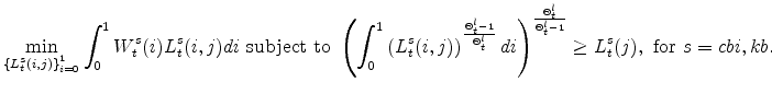
There are a number of market clearing conditions that must be satisfied in our model. Market clearing in the slow-growing "consumption" goods and fast-growing "capital" goods sectors, given price- and wage-adjustment costs and variable utilization costs, implies that

$\displaystyle X^{cbi}_{t}$	$\displaystyle =$	$\displaystyle \int_{0}^{1} E^{cnn}_{t}(i)di + \int_{0}^{1} E^{r}_{t}(k)dk + \widetilde{X}^{HG}_{t}Z^{m}_{t}\left(Z^{kb}_{t}\right)^{\alpha}$
	$\displaystyle +$	$\displaystyle \frac{100\cdot\chi^{p}}{2} \left(\Pi^{p,kb}_{t} - \eta^{p}\Pi^{p,cbi}_{t-1} - (1 - \eta^{p})\Pi^{p,cbi}_{\ast}\right)^{2} P^{cbi}_{t}X^{cbi}_{t}$
	$\displaystyle +$	$\displaystyle \frac{100 \cdot \chi^{w}}{2} \left(\Pi^{w,cbi}_{t} % - \eta^{w}\Pi^{w,cbi}_{t-1} - (1 - \eta^{w})\Pi^{w,cbi}_{\ast}\right)^{2} % W^{cbi}_{t}L^{cbi}_{t} - \kappa\left(\frac{U^{cbi}_{t}(k)^{1+\psi} -% 1}{1+\psi} \right) P^{cbi}_{t}K^{nr,cbi}_{t}$	(19)

and

$\displaystyle X^{kb}_{t}$	$\displaystyle =$	$\displaystyle \int_{0}^{1} E^{cd}_{t}(k)dk + \int_{0}^{1} E^{nr}_{t}(k)dk + \widetilde{X}^{HG}_{t}Z^{m}_{t}Z^{kb}_{t}$
	$\displaystyle +$	$\displaystyle +\frac{100\cdot\chi^{p}}{2} \left(\Pi^{p,kb}_{t} - \eta^{p}\Pi^{p,kb}_{t-1} - (1 - \eta^{p})\Pi^{p,kb}_{\ast}\right)^{2} P^{kb}_{t}X^{kb}_{t}$
	$\displaystyle +$	$\displaystyle \frac{100 \cdot \chi^{w}}{2} \left(\Pi^{w,kb}_{t} % - \eta^{w}\Pi^{w,kb}_{t-1} - (1 - \eta^{w})\Pi^{w,kb}_{\ast}\right)^{2} W^{kb}_{t}L^{kb}_{t} - \kappa\left(\frac{U^{kb}_{t}(k)^{1+\psi} - 1}{1+\psi} \right) P^{kb}_{t}K^{nr,kb}_{t} . \ \ \ \ \ \ \ \$	(20)

The market clearing conditions for the labor and non-residential capital supplied and demanded in sector are given by

$\displaystyle L^{s}_{t}(i)= \int_{0}^{1} L^{s}_{t}(i,j)dj \ {\mathrm{and}}\ \int_{0}^{1} U(k)^{s}_{t}K^{nr,s}_{t}(k)dk= \int_{0}^{1} K^{u,nr,s}_{t}(j)dj \ \forall \ i \in [0,1]\ {\mathrm{and\ for}}\ s=cbi,kb.$

(21)

The market clearing conditions for consumer durables and residential capital are

$\displaystyle \int_{0}^{1} K^{cd}_{t}(k)dk= \int_{0}^{1} K^{cd}_{t}(i)di \ {\mathrm{and}}\ \int_{0}^{1} K^{r}_{t}(k)dk= \int_{0}^{1} K^{r}_{t}(i)di.$

(22)

1.9 Inflation

The identities for inflation include:

$\displaystyle W^{s}_{t}(i)= \Pi^{w,s}_{t}(i)W^{s}_{t-1}(i) \$	$\displaystyle {\mathrm{and}}%$	$\displaystyle \ W^{s}_{t}= \Pi^{w,s}_{t}W^{s}_{t-1} \ \forall \ i \in [0,1]\ {% \mathrm{and \ for}}\ s=cbi,kb, \ {\mathrm{and}}\ \ \ \ \ \$	(23)
$\displaystyle P^{s}_{t}(j)= \Pi^{p,s}_{t}(j)P^{s}_{t-1}(j) \ \ \$	$\displaystyle {\mathrm{and}}%$	$\displaystyle \ P^{s}_{t}= \Pi^{p,s}_{t}P^{s}_{t-1} \ \ \ \forall \ j \in [0,1]\ {% \mathrm{and \ for}}\ s=cbi,kb.\ \$	(24)

2 Equilibrium

Before characterizing equilibrium in this model, we define three additional variables: The price of installed non-residential capital $Q^{nr}_{t}(k)$ ; the price of installed consumer durables capital $Q^{cd}_{t}(k)$ ; and the price of installed residential capital $Q^{r}_{t}(k)$ . These variables are the lagrange multiplier on the capital evolution equations that would be implied by the th capital owner's profit-maximization problems.

Equilibrium in our model is an allocation:

		$\displaystyle \left\{H^{gdp}_{t} , X^{cbi}_{t} ,\{X^{cbi}_{t}(j)\}_{j=0}^{1}, X^{kb}_{t} ,\{X^{kb}_{t}(j)\}_{j=0}^{1}, \{E^{nr}_{t}(k)\}_{k=0}^{1},\{E^{r}_{t}(k)\}_{k=0}^{1},\{E^{cd}_{t}(k)% \}_{k=0}^{1}, \right. \ \ \ \$
		$\displaystyle \{E^{cnn}_{t}(i)\}_{i=0}^{1}, \{\Lambda^{r}_{t}(i)\}_{i=0}^{1}, \{\Lambda^{cd}_{t}(i)\}_{i=0}^{1},\{\Lambda^{cnn}_{t}(i)\}_{i=0}^{1}, \{\Lambda^{l,cbi}_{t}(i)\}_{i=0}^{1},\{\Lambda^{l,kb}_{t}(i)\}_{i=0}^{1},$
		$\displaystyle \{L^{cbi}_{t}(i)\}_{i=0}^{1},\{\{L^{cbi}_{t}(i,j)\}_{i=0}^{1}\}_{j=0}^{1}, \{L^{kb}_{t}(i)\}_{i=0}^{1},\{\{L^{kb}_{t}(i,j)\}_{i=0}^{1}\}_{j=0}^{1}, \{U^{cbi}_{t}(j)\}_{j=0}^{1},\{U^{kb}_{t}(j)\}_{j=0}^{1},$
		$\displaystyle \{K^{u,nr,cbi}_{t}(j)\}_{j=0}^{1},\{K^{u,nr,kb}_{t}(j)\}_{j=0}^{1}, \{K^{nr,cbi}_{t}(k)\}_{k=0}^{1},\{K^{nr,kb}_{t}(k)\}_{k=0}^{1},% \{K^{nr}_{t+1}(k)\}_{k=0}^{1},$
		$\displaystyle \ \ \ \ \ \ \ \ \ \ \ \ \ \ \ \ \ \ \ \ \ \ \ \ \ \ \ \ \ \ \ \ \ \ \ \ \ \ \ \ \left. \{K^{r}_{t+1}(k)\}_{k=0}^{1},\{K^{r}_{t+1}(i)\}_{i=0}^{1}, \{K^{cd}_{t+1}(k)\}_{k=0}^{1},\{K^{cd}_{t+1}(i)\}_{i=0}^{1} \right\}_{t=0}^{\infty}$

and a sequence of values

		$\displaystyle \left\{\Pi^{c}_{t} , \Pi^{p,cbi}_{t} ,\{\Pi^{p,cbi}_{t}(j)\}_{j=0}^{1}, \Pi^{p,kb}_{t} ,\{\Pi^{p,kb}_{t}(j)\}_{j=0}^{1}, \Pi^{w,cbi}_{t} ,\{\Pi^{w,cbi}_{t}(i)\}_{j=0}^{1}, \Pi^{w,kb}_{t} ,\{\Pi^{w,kb}_{t}(i)\}_{j=0}^{1}, \right.$
		$\displaystyle \frac{P^{kb}_{t}}{P^{cbi}_{t}},\left\{\frac{P^{kb}_{t}(j)}{% P^{cbi}_{t}}\right\}_{j=0}^{1} , \frac{W^{cbi}_{t}}{P^{cbi}_{t}},\left\{% \frac{W^{cbi}_{t}(i)}{P^{cbi}_{t}}\right\}_{i=0}^{1} , \frac{W^{kb}_{t}}{% P^{cbi}_{t}},\left\{\frac{W^{kb}_{t}(i)}{P^{cbi}_{t}}\right\}_{i=0}^{1} , \frac{R^{nr,cbi}_{t}}{P^{cbi}_{t}},\frac{R^{nr,kb}_{t}}{P^{cbi}_{t}}, \frac{% R^{nr}_{t}}{P^{cbi}_{t}},$
		$\displaystyle \left. \frac{R^{r}_{t}}{P^{cbi}_{t}}, \frac{R^{cd}_{t}}{% P^{cbi}_{t}}, \left\{\frac{MC^{cbi}_{t}(j)}{P^{cbi}_{t}}\right\}_{j=0}^{1} % , \left\{\frac{MC^{kb}_{t}(j)}{P^{cbi}_{t}}\right\}_{j=0}^{1} , \left\{% \frac{Q^{nr}_{t}(k)}{P^{cbi}_{t}}\right\}_{k=0}^{1} , \left\{\frac{% Q^{r}_{t}(k)}{P^{cbi}_{t}}\right\}_{k=0}^{1} , \left\{\frac{Q^{cd}_{t}(k)% }{P^{cbi}_{t}}\right\}_{k=0}^{1} ,R_{t} \right\}_{t=0}^{\infty}$

that satisfy the following conditions:

The model's two representative final-good producing firms solve (1) for and ;
All intermediate-good producers $j \in [0,1]$ solve (3), (5), and (7) for and ;
All capital owners $k \in [0,1]$ solve (8), (10), and (11);
All households $i \in [0,1]$ solve (12);
The two final goods markets clear as in (19) and (20);
All intermediate goods markets clear;
The labor and non-residential capital markets clear as in (21);
The consumer durable and residential capital rental markets clear as in (22);
The identities given in (23) hold;
The identities given in (24) hold;
The monetary authority follows (15) and (17).

In solving these problems agents take as given the initial values of all (lagged) endogenous state variables (e.g., capital stocks, etc.) and the sequence of exogenous variables

$\displaystyle \left\{ \Gamma^{z,kb}_{t} ,\Gamma^{z,m}_{t} , \Theta^{cbi}_{t} ,\Theta^{kb}_{t} , \Theta^{l}_{t} , A^{nr}_{t} ,A^{r}_{t},A^{cd}_{t} ,\Omega_{t} , X^{HG}_{t} \right\}_{t=0}^{\infty}$

implied by the sequence of shocks

$\displaystyle \left\{ \epsilon^{z,kb}_{t} ,\epsilon^{z,m}_{t} , \epsilon^{\theta,cbi}_{t} ,\epsilon^{\theta,kb}_{t} , \epsilon^{\theta,l}_{t} , \epsilon^{a,nr}_{t} ,\epsilon^{a,r}_{t} ,\epsilon^{a,cd}_{t} , \epsilon^{\omega}_{t} , \epsilon^{HG}_{t} , \epsilon^{r}_{t} \right\}_{t=0}^{\infty}.$

We estimate the log-linearized, symmetric and stationary version of the model described above. Equilibrium in the symmetric and stationary version of the model is defined in appendix A. The log-linearization of our model equations is performed symbolically by the software that we use to parse the model into its estimable form. The steady-state solution to the symmetric and stationary version of the model is an input into the model's estimation and is presented in appendix B.

3 Estimation

3.1 Data

The empirical implementation of the model takes a log-linear approximation to the first-order conditions and constraints that describe the economy's equilibrium, casts this resulting system in its state-space representation for the set of (in our case 11) observable variables, uses the Kalman filter to evaluate the likelihood of the observed variables, and forms the posterior distribution of the parameters of interest by combining the likelihood function with a joint density characterizing some prior beliefs. Since we do not have a closed-form solution of the posterior, we rely on Markov-Chain Monte Carlo (MCMC) methods.

The model is estimated using 11 data series over the sample period from 1984:Q4 to 2008:Q4. The series are:

The growth rate of real gross domestic product;
The growth rate of real consumption expenditure on non-durables and services excluding housing services;
The growth rate of real consumption expenditure on durables;
The growth rate of real residential investment expenditure;
The growth rate of real business investment expenditure;
Consumer price inflation, as measured by the growth rate of the Personal Consumption Expenditure (PCE) price index;
Consumer price inflation, as measured by the growth rate of the PCE price index excluding food and energy prices;
Inflation for consumer durable goods, as measured by the growth rate of the PCE price index for durable goods;
Hours, which equals hours of all persons in the non-farm business sector from the Bureau of Labor Statistics;¹
The growth rate of real wages, as given by compensation per hour in the non-farm business sector from the Bureau of Labor Statistics divided by the GDP price index;
The federal funds rate.

Our implementation adds measurement error processes to the likelihood implied by the model for all of the observed series used in estimation except the nominal interest rate series.

3.2 Model Parameters

The model' calibrated parameters are presented in Table 1, while the estimated parameters are presented in Tables 3 and 4. We based out decision on several considerations. First, some important determinants of steady-state behavior were calibrated to yields growth rates of GDP and associated price indexes that corresponded to "conventional" wisdom in policy circles, even though slight deviations from such values would have been preferred (in a "statistically significant" way) to our calibrated values. In other cases, parameters were calibrated based on how informative the data were likely to be on the parameter and/or identification and overparameterization issues. Finally, the standard deviations of the measurement error assumed in the observables was chosen to ensure a moderate contribution of such errors to the variability in the data (according to our model) while also preserving desirable forecast properties; we present the observables and the role of measurment error in the results below.

The first three columns of Table 3 and 4 outline our assumptions about the prior distributions of the estimated parameters, the remaining columns describe the parameters' posterior distributions, which we now proceed to discuss.

We consider first the parameters related to household and business spending decisions. The habit-persistence parameter is moderate, near 0.6.²Investment adjustment costs are large for residential investment but small for business investment. This finding highlights once advantage of our disaggregated approach. In addition, this result is importantly driven by the inclusion of inventory investment in business investment; this is a very cyclically important component of GDP and was an important element in early investigations of dynamic general equilbrium models (e.g., Kydland and Prescott (1982)), but is typically ignored in similar DSGE models.

The estimated value of the inverse of the labor supply elasticity implies quite elastic labor supply. We also find a role for the sectoral adjustment costs to labor: In our multisector setup, shocks to productivity or preferences in one sector of the economy result in strong shifts of labor towards that sector, which conflicts with the high degree of sectoral co-movement in the data.

Finally, adjustment costs to prices and wages are both estimated to be important. Our estimate of the price adjustment cost is equivalent to a Calvo pricing setting where a bit more than half of the firms cannot update their prices each period. The estimated quadratic costs in wages imply a slightly larger frequency of adjustments for the suppliers of labor. We also find only a modest role for lagged inflation in our adjustment cost specification (around 1/4), equivalent to modest indexation to lagged inflation in other sticky-price specifications. This differs from some other estimates, perhaps because of the focus on a more recent post-1983 sample (similar to results in [Kiley (2007)] and [Laforte (2007)]).

3.3 Variance Decompositions

Tables 5 and 6 present forecast error variance decompositions at various (quarterly) horizons at the posterior mode of the parameter estimates for key variables and shocks. We run through the key results here.

Volatility in aggregate GDP growth is accounted for primarily by the technology shocks in each sector, although the economy-wide risk premium shock contributes non-negligibly to the unconditional variance of GDP growth.

Volatility in hours per capita is accounted for primarily by the economy-wide risk premium and business investment risk premium shocks at horizons between one and sixteen quarters. Technology shocks in each sector contribute appreciably to the unconditional variance. The large role for risk premia shocks in the forecast error decomposition at business cycle horizons illustrates the importance of this type of "demand" shock for volatility in the labor market. This result is notable, as hours per capita is the series most like a "gap" variable in the model - that is, house per capita shows persistent cyclical fluctuations about its trend value.

Volatility in core inflation is accounted for primarily by the markup shocks in the short run and technology shocks in the long run.

Volatility in the federal funds rate is accounted for primarily by the economywide risk premium.

Volatility in expenditures on consumer non-durables and non-housing services is, in the near horizon, accounted for predominantly by economy-wide and non-residential investment specific risk-premia shocks. In the far horizon, volatility is accounted for primarily by capital-specific and economy-wide technology shocks.

Volatilities in expenditures on consumer durables, residential investment, and non-residential investment are, in the near horizon, accounted for predominantly by their own sector specific risk-premium shocks. At farther horizons, their volatilities are accounted for by capital-specific technology shocks.

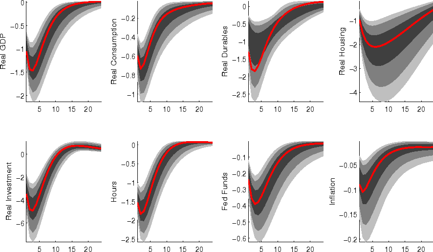
3.4 Impulse Responses

We now turn to the impulse responses of some of the key observable variables to the exogenous shocks that drive fluctuations in the model. In each case we consider unit shocks; the reader is referred to the reported estimates of the standard deviation of the shocks for information that will scale these responses to units consistent with a standard deviation shock. Expenditure variables are reported as percent deviations from initial values (in natural log points); inflation variables and the federal funds rate are reported at quarterly (not annual) rates.

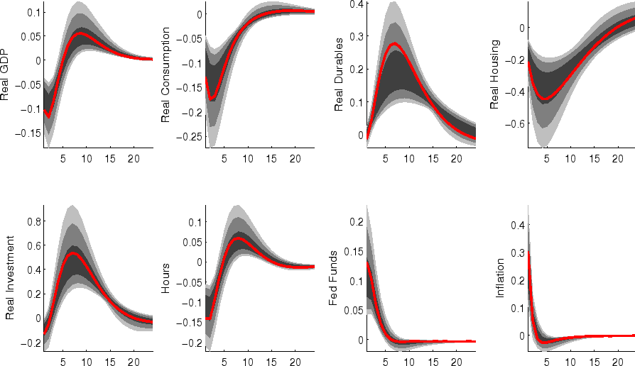
The impulse responses to a monetary policy innovation (shown in figure 5) captures the conventional wisdom regarding the effects of such shocks. In particular, both household and business expenditures on durables (consumer durables, residential investment, and nonresidential investment) respond strongly (and with a hump-shape) to a contractionary policy shock, with more muted responses by nondurables and services consumption; each measure of inflation responds gradually, albeit more quickly than in some analyses based on vector autoregressions (VARs). (This difference between VAR-based and DSGE-model based impulse responses has been highlighted elsewhere - for example, in the survey of Boivin, Kiley, and Mishkin (2010)).

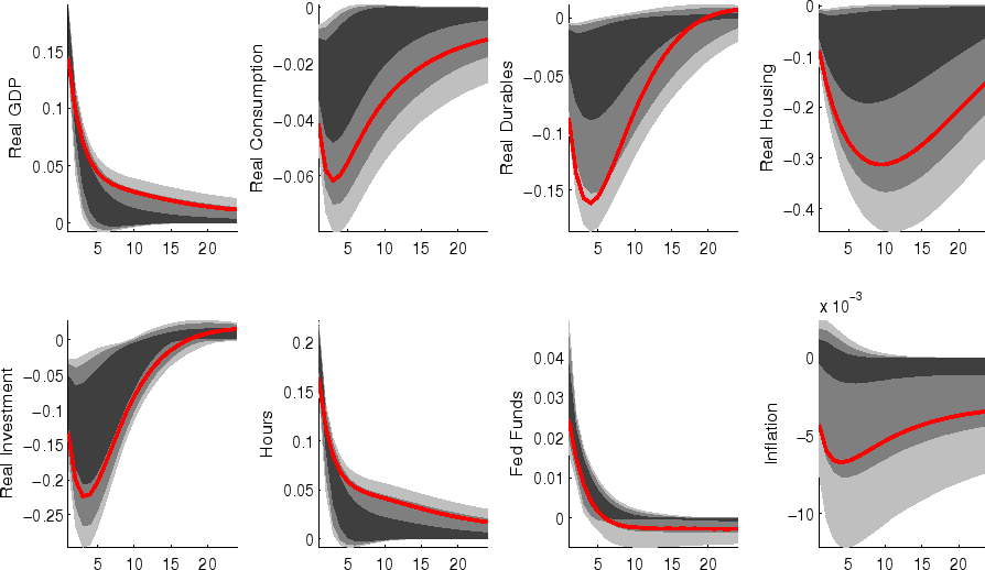
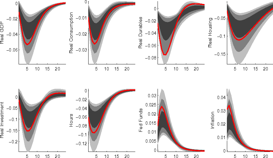
Figures 2 to 7 present the impulse responses of key variables to the model's four risk premia shocks ( $\Omega_{t}$ , $A^{nr}_{t}$ , $A^{cd}_{t}$ , and $A^{r}_{t}$ ), the autonomous spending shock ( $X^{HG}$ ), price and wage mark-up shocks ( $\Theta^{cbi}_{t}$ , $\Theta^{cbi}_{t}$ , and $\Theta^{l}_{t}$ ), and technology shocks ( $\Gamma^{z,m}_{t}$ and $% \Gamma^{z,kb}_{t}$ ).

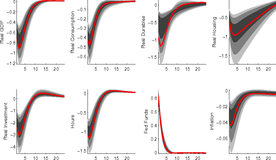
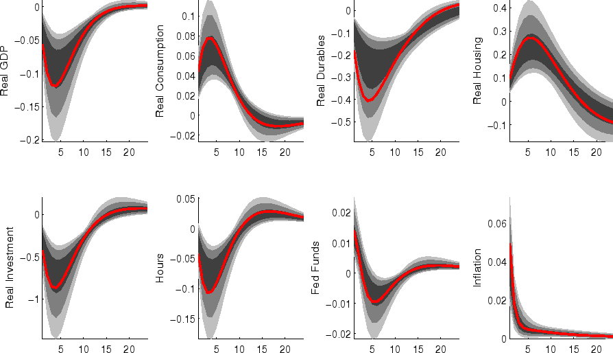
The aggregate risk premium shock (figure 2) depresses spending across the board, lowering hours appreciably; inflation and the federal funds rate fall in response. (As in the model of Smets and Wouters (2007), the aggregate risk premium drives down the flexible-price nominal interest rate one-for-one, and hence the downward move in the nominal funds rate facilitates moving the economy toward its flexible price outcome).

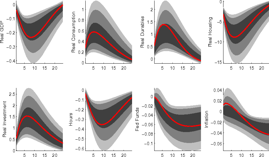
Shocks to sectoral risk premia (figures 10, 11 and 12) principally depress spending in the associated category of expenditure, with offsetting positive effects on other spending (which is "crowded in").

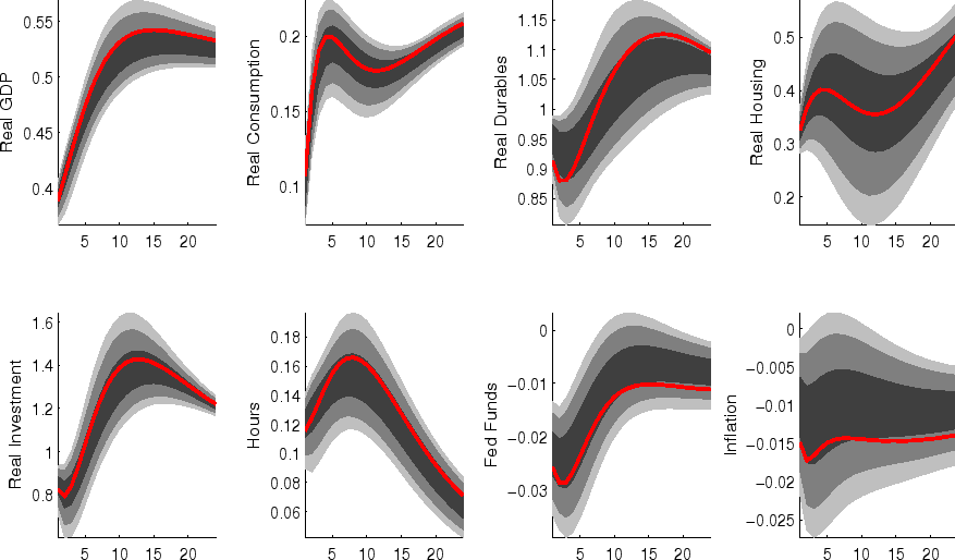
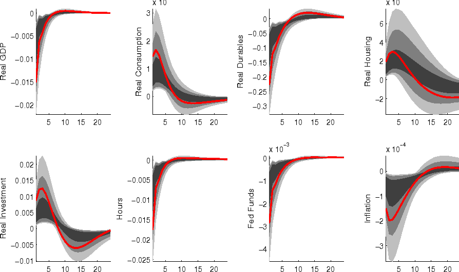
The impulse responses to a capital-specific technology shock (shown in figure 6) are a touch more gradual, as the embodied component of this type of technological progress implies a need for nonresidential capital accumulation. (In addition, the long-run responses of nonresidential investment and consumer durables are much larger than those of other spending, reflecting the biased nature of this technology shock).

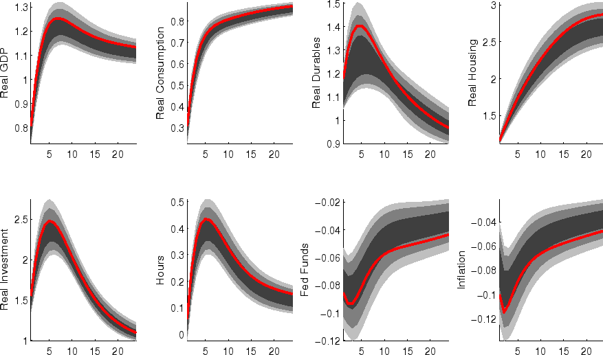
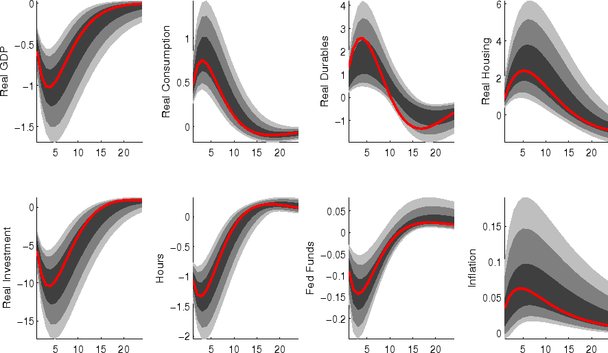
Following an economy-wide technology shock (figure 7), output rises gradually to its long-run level; hours respond relatively little to the shock (in comparison to, for example, output, reflecting both the influence of stick prices and wages and the offsetting income and substitution effects of such a shock on households willingness to supply labor.

3.5 Implied Paths

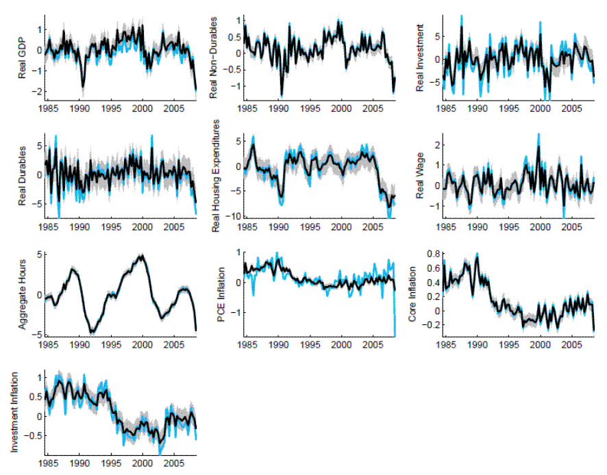
Figure 13 presents the observed data (in blue) and the observable data net of the model's estimated measurement error (in black), along 95 percent confidence intervals. For series other than overall PCE price inflation, measurement error is a moderate portion of movements in the series. The larger role for measurement error in accounting for the path of PCE price inflation reflects the absence of separate sectors for food and energy in the model.

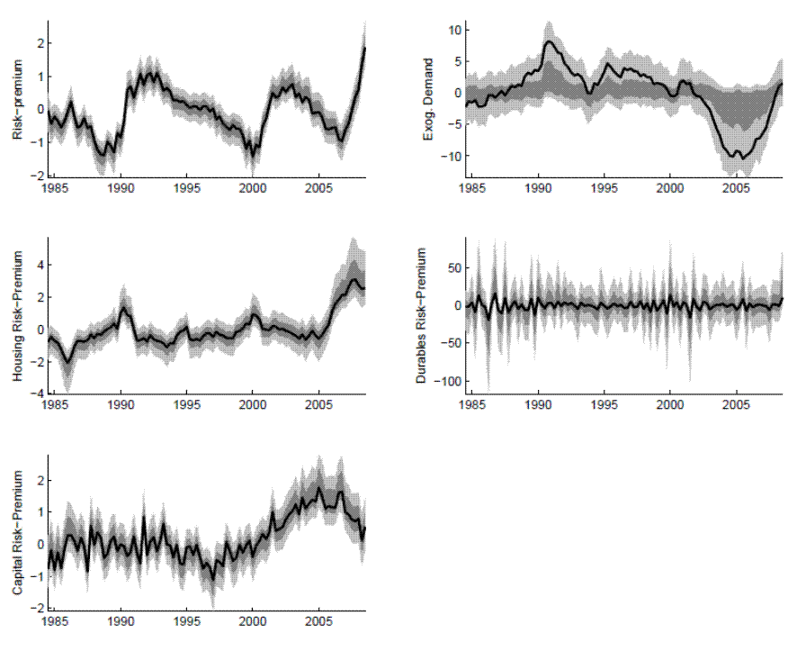
Figures 14 and 15 report modal estimates of the model's structural shocks and the persistent exogenous drivers (i.e., risk premia and autonomous demand). These series have recognizable patterns for those familiar with U.S. economic fluctuations. For example, the risk premia jump at the end of the sample, reflecting the financial crisis and the model's identification of risk premia, both economy-wide and for housing, as key drivers. In addition, the large negative value for autonomous demand around 2005 reflects the widening of the current account deficit: While this factor is absent from our closed-economy model, the use of economywide data picks up the drag from demand other than demand for U.S. produced goods and services.³

Of course, these stories from a glance at the exogenous drivers yield applications for alternative versions of the EDO model and future model enhancements. For example, the exogenous risk premia can easily be made to have an endogenous component following the approach of Bernanke, Gertler, and Gilchrist (1999) (and indeed we have considered models of that type). At this point we view incorporation of such mechanisms in our baseline approach as premature, pending ongoing research on financial frictions, banking, and intermediation in dynamic general equilibrium models. Nonetheless, the EDO model captured the key financial disturbances during the last several years in its current specification, and examining the endogenous factors that explain these developments will be a topic of further study.

4 Summing up

This paper has presented documentation for the large-scale estimated EDO model of the U.S. economy used for projections and policy analysis at the Federal Reserve Board. Cyclical dynamics are mostly accounted for by shocks to risk premia (e.g., see the discussion of output gaps in Kiley (2010b)). The integration of business cycle and growth facts in a two-sector model with investment-specific technological progress also allows consideration of key drivers of productivity and long-run growth. Ongoing research examines a range of issues related to the sources of economic fluctuations, financial frictions, and the design of monetary and fiscal policy (e.g., at the zero lower bound).

Bibliography

Bernanke, B., M. Gertler, and S. Gilchrist., 1999.

The financial accelerator in a quantitative business cycle framework, In: John B. Taylor and Michael Woodford, Editor(s), Handbook of Macroeconomics, Elsevier, 1999, Volume 1, Part 3, Pages 1341-1393.

Beveridge, S. and C.R. Nelson., 1981.

A new approach to the decomposition of economic time series into permanent and transitory components with particular attention to measurement of the business cycle, Journal of Monetary Economics 7, 151-174.

Boivin, J., M. Kiley, and F.S. Mishkin., 2010.

How Has the Monetary Transmission Mechanism Evolved Over Time? Forthcoming in B. Friedman and M. Woodford, eds., The Handbook of Monetary Economics, Elsevier.

Edge, R., Kiley, M., Laforte, J.P., 2008.

Natural rate measures in an estimated DSGE model of the U.S. economy. Journal of Economic Dynamics and Control 32:2512â€“2535.

Edge, R., Kiley, M., Laforte, J.P., 2010.

A comparison of forecast performance between Federal Reserve staff forecasts, simple reduced-form models, and a DSGE model. Forthcoming in Journal of Applied Econometrics.

Kiley, M., 2007.

A Quantitative Comparison of Sticky-Price and Sticky-Information Models of Price Setting. Journal of Money, Credit, and Banking 39, 101-25.

Kiley, M., 2010a.

Habit Persistence, Non-separability between Consumption and Leisure, or Rule-of-Thumb Consumers: Which Accounts for the Predictability of Consumption Growth? Forthcoming in The Review of Economics and Statistics.

Kiley, M., 2010b.

Output Gaps. Forthcoming in Federal Reserve Board Finance and Economics Discussion Series (FEDS).

Kydland, Finn and Prescott, Edward., 1982.

Time-to-build and Aggregate Fluctuations. Econometrica, 50, 6,1345 - 1370.

Laforte, J., 2007.

Pricing Models: A Bayesian DSGE Approach to the U.S. Economy. Journal of Money, Credit, and Banking 39, 127-54.

Smets, F., Wouters, R., 2007.

Shocks and Frictions in the US Busines Cycles: A Bayesian DSGE Approach. American Economic Review, American Economic Association, vol. 97(3), pages 586-606, June.

A. Equilibrium in the Symmetric and Stationary Model

The symmetric equilibrium is an allocation:

		$\displaystyle \left\{H^{gdp}_{t}, \widetilde{X}^{cbi}_{t},\widetilde{X}% ^{kb}_{t}, \widetilde{E}^{nr}_{t},\widetilde{E}^{r}_{t}, \widetilde{E}% ^{cd}_{t}, \widetilde{E}^{cnn}_{t}, \widetilde{\Lambda}^{r}_{t},\widetilde{% \Lambda}^{cd}_{t},\widetilde{\Lambda}^{cnn}_{t}, \Lambda^{l,cbi}_{t},\Lambda^{l,kb}_{t}, \right.$
		$\displaystyle \ \ \ \ \ \ \ \ \ \ \ \ \left. L^{cbi}_{t},L^{kb}_{t},U^{cbi}_{t},U^{kb}_{t}, \widetilde{K}^{u,nr,cbi}_{t},% \widetilde{K}^{u,nr,kb}_{t}, \widetilde{K}^{nr,cbi}_{t},\widetilde{K}% ^{nr,kb}_{t},\widetilde{K}^{nr}_{t+1}, \widetilde{K}^{r}_{t+1},\widetilde{K}% ^{cd}_{t+1} \right\}_{t=0}^{\infty}$

and a sequence of values

		$\displaystyle \left\{\Pi^{c}_{t}, \Pi^{p,cbi}_{t},\Pi^{p,kb}_{t}, \Pi^{w,cbi}_{t},\Pi^{w,kb}_{t}, \widetilde{P}% ^{kb}_{t},\widetilde{W}^{cbi}_{t},\widetilde{W}^{kb}_{t}, \right.$
		$\displaystyle \ \ \ \ \ \ \ \ \left. \widetilde{R}^{nr,cbi}_{t},\widetilde{R}% ^{nr,kb}_{t}, \widetilde{R}^{nr}_{t},\widetilde{R}^{r}_{t}, \widetilde{R}% ^{cd}_{t},\widetilde{MC}^{cbi}_{t},\widetilde{MC}^{kb}_{t}, \widetilde{Q}% ^{nr}_{t},\widetilde{Q}^{r}_{t},\widetilde{Q}^{cd}_{t},R_{t} \right\}_{t=0}^{\infty}$

that satisfy the symmetric and stationary versions of the first-order conditions implied by the decisions problems of firms and households outlined in the main text, taking as given the initial values of the endogenous states and the sequence of exogenous variables

$\displaystyle \left\{ \Gamma^{z,kb}_{t} ,\Gamma^{z,m}_{t} , \Theta^{cbi}_{t} ,\Theta^{kb}_{t} ,\Theta^{l}_{t}, A^{nr}_{t} ,A^{r}_{t},A^{cd}_{t} ,\Omega_t ,\widetilde{X}^{HG}_{t} \right\}_{t=0}^{\infty}$

implied by the sequence of shocks

$\displaystyle \left\{ \epsilon^{z,kb}_{t} ,\epsilon^{z,m}_{t} , \epsilon^{\theta,cbi}_{t} ,\epsilon^{\theta,kb}_{t} ,\epsilon^{\theta,l}_{t} , \epsilon^{a,nr}_{t} ,\epsilon^{a,r}_{t} ,\epsilon^{a,cd}_{t} ,\epsilon^{\omega}_{t} \epsilon^{HG}_{t} ,\epsilon^{R}_{t} \right\}_{t=0}^{\infty}.$

The stationary versions of the model's key equations are presented in this section. Note also that definitions for all of the model's stationary variables can be found in appendix F.

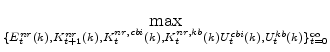
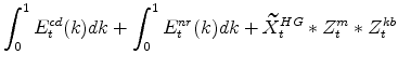
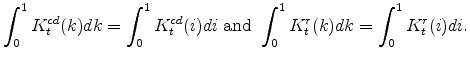
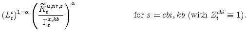
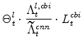
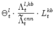
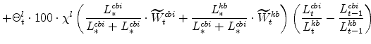
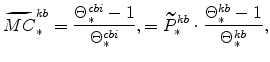
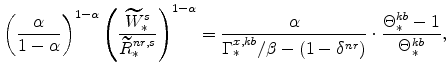
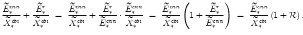
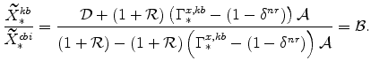
The symmetric and stationary first-order conditions implied by the second step of the intermediate-goods producing firms' cost minimization problems (equation 5) are:

$\displaystyle L^{s}_{t}$	$\displaystyle =$	$\displaystyle \left(1-\alpha\right) \cdot \widetilde{X}% ^{s}_{t} \cdot \frac{\widetilde{MC}^{s}_{t}}{\widetilde{W}^{s}_{t}} \ \ \ \ \ \ \ \ \ \ \ \ \ \ \ \ \ \ \ \ \ \ \ \ \ \ \ \ \mathrm{for} \ s=cbi,kb$	(25)
$\displaystyle \frac{\widetilde{K}^{u,nr,s}_{t}}{\Gamma^{x,kb}_{t}}$	$\displaystyle =$	$\displaystyle \alpha \cdot \widetilde{X}^{s}_{t} \cdot \frac{\widetilde{MC}^{s}_{t}}{% \widetilde{R}^{nr,s}_{t}} \ \ \ \ \ \ \ \ \ \ \ \ \ \ \ \ \ \ \ \ \ \ \ \ \ \ \ \ \ \ \ \ \ \ \ \ \mathrm{for} \ s=cbi,kb.$	(26)
$\displaystyle \widetilde{X}^{s}_{t}$	$\displaystyle =$	$\displaystyle \left(L^{s}_{t}\right)^{1-\alpha} \left(\frac{\widetilde{K}^{u,nr,s}_{t}}{\Gamma^{x,kb}_{t}}\right)^{\alpha} \ \ \ \ \ \ \ \ \ \ \ \ \ \ \ \ \ \ \ \ \mathrm{for} \ s=cbi,kb\ (% \mathrm{with} \ Z^{cbi}_{t}\equiv 1).$	(27)

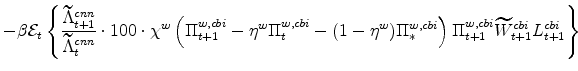
The stationary price Phillips curves that are implied by the intermediate-goods producing firms' profit maximization problems (equation7) are

$\displaystyle \Theta^{cbi}_{t}\widetilde{MC}^{cbi}_{t}\widetilde{X}^{cbi}_{t}$	$\displaystyle =$	$\displaystyle \left(\Theta^{cbi}_{t}-1\right)\widetilde{X}% ^{cbi}_{t}$
	$\displaystyle +$	$\displaystyle 100\cdot\chi^{p} \left(\Pi^{p,cbi}_{t} - \eta^{p}\Pi^{p,cbi}_{t-1} - (1 - \eta^{p})\Pi^{p,cbi}_{\ast}\right) \Pi^{p,cbi}_{t}\widetilde{X}% ^{cbi}_{t}$
	$\displaystyle -$	$\displaystyle \beta \mathcal{E}_{t} \left\{\frac{\widetilde{\Lambda}% ^{cnn}_{t+1}}{\widetilde{\Lambda}^{cnn}_{t}}\cdot 100 \cdot \chi^{p} \left(\Pi^{p,cbi}_{t+1} - \eta^{p}\Pi^{p,cbi}_{t} - (1 - \eta^{p})\Pi^{p,cbi}_{\ast}\right) \Pi^{p,cbi}_{t+1}\widetilde{X}% ^{cbi}_{t+1} \right\} \ \ \ \ \ \$	(28)
$\displaystyle \Theta^{kb}_{t}\widetilde{MC}^{kb}_{t}\widetilde{X}^{kb}_{t}$	$\displaystyle =$	$\displaystyle \left(\Theta^{kb}_{t}-1\right)\widetilde{P}% ^{kb}_{t}\widetilde{X}^{kb}_{t}$
	$\displaystyle +$	$\displaystyle 100\cdot\chi^{p}\left(\Pi^{p,kb}_{t} - \eta^{p}\Pi^{p,kb}_{t-1} - (1 - \eta^{p})\Pi^{p,kb}_{\ast}\right) \Pi^{p,kb}_{t}\widetilde{P}% ^{kb}_{t} \widetilde{X}^{kb}_{t}$
	$\displaystyle -$	$\displaystyle \beta \mathcal{E}_{t} \left\{\frac{\widetilde{\Lambda}% ^{cnn}_{t+1}}{\widetilde{\Lambda}^{cnn}_{t}}\cdot 100 \cdot \chi^{p} \left(\Pi^{p,kb}_{t+1} - \eta^{p}\Pi^{p,kb}_{t} - (1 - \eta^{p})\Pi^{p,kb}_{\ast}\right) \Pi^{p,kb}_{t+1}\widetilde{P}% ^{kb}_{t+1}\widetilde{X}^{kb}_{t+1} \right\} \ \ \ \ \ \$	(29)

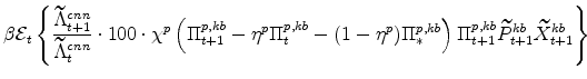
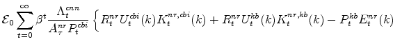
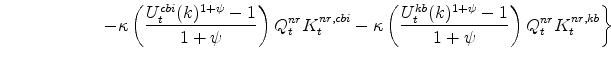
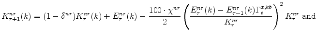
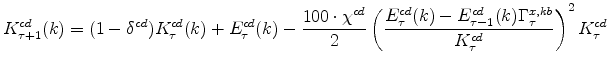
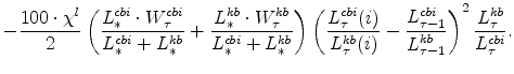
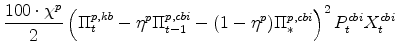
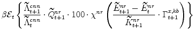
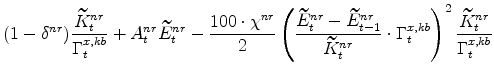
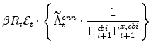
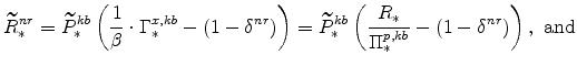
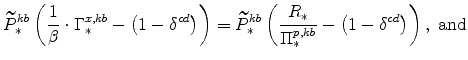
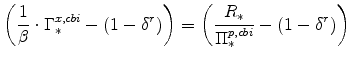
The symmetric and stationary first-order conditions implied by the non-residential part of the capital owners' profit-maximization problem (equation 8) are:

$\displaystyle \widetilde{Q}^{nr}_{t}$

$\displaystyle =$

$\displaystyle \beta \mathcal{E}_{t} \left\{\frac{% \widetilde{\Lambda}^{cnn}_{t+1}}{\widetilde{\Lambda}^{cnn}_{t}} \cdot\frac{1}{\Gamma^{x,kb}_{t+1}} \left(\widetilde{R}^{nr}_{t+1}+(1-\delta^{nr})% \widetilde{Q}^{nr}_{t+1} \right)\right\}$

(30)

$\displaystyle \widetilde{R}^{nr,s}_{t}$	$\displaystyle =$	$\displaystyle \frac{\widetilde{R}^{nr}_{t}}{% U^{s}_{t}} \ \ \ \ \ \ \ \ \ \ \ \ \ \ \ \ \ \ \ \ \ \ \ \ \ \ \ \ \ \ \ \ \ \ \ \ \ \ \ \ \ \ \ \ \ \ \ \ \ \ \ \ \ \ \ \ \ \ \ \ \ \ \ \ \ \mathrm{for} \ s=cbi,kb$	(31)
$\displaystyle U^{s}_{t}$	$\displaystyle =$	$\displaystyle \left(\frac{1}{\kappa}\cdot\frac{\widetilde{R}% ^{nr,s}_{t}}{\widetilde{Q}^{nr}_{t}}\right)^{\frac{1}{\psi}} \ \ \ \ \ \ \ \ \ \ \ \ \ \ \ \ \ \ \ \ \ \ \ \ \ \ \ \ \ \ \ \ \ \ \ \ \ \ \ \ \ \ \ \ \ \ \ \ \ \ \ \ \mathrm{for} \ s=cbi,kb$	(32)
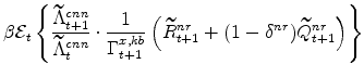
$\displaystyle \widetilde{P}^{kb}_{t}$	$\displaystyle =$	$\displaystyle \widetilde{Q}^{nr}_{t} \left[% A^{nr}_{t}-100\cdot\chi^{nr} \left(\frac{\widetilde{E}^{nr}_{t} - \widetilde{E}^{nr}_{t-1}} {\widetilde{K}^{nr}_{t}}\cdot \Gamma^{x,kb}_{t}\right) \right]$
	$\displaystyle +$	$\displaystyle \beta \mathcal{E}_{t} \left\{ \frac{\widetilde{\Lambda }^{cnn}_{t+1}}{\widetilde{\Lambda}^{cnn}_{t}}\cdot \widetilde{Q}% ^{nr}_{t+1} \cdot 100 \cdot \chi^{nr} \left(\frac{\widetilde{E}% ^{nr}_{t+1} - \widetilde{E}^{nr}_{t}} {\widetilde{K}^{nr}_{t+1}}% \cdot\Gamma^{x,kb}_{t+1}\right)\right\}$	(33)
$\displaystyle \widetilde{K}^{nr}_{t+1}$	$\displaystyle =$	$\displaystyle (1 - \delta^{nr})\frac{% \widetilde{K}^{nr}_{t}}{\Gamma^{x,kb}_{t}} + A^{nr}_{t}\widetilde{E}% ^{nr}_{t} - \frac{100\cdot\chi^{nr}}{2} \left(\frac{\widetilde{E}% ^{nr}_{t} - \widetilde{E}^{nr}_{t-1}}{\widetilde{K}^{nr}_{t}} \cdot\Gamma^{x,kb}_{t}\right)^{2} \frac{\widetilde{K}^{nr}_{t}}{% \Gamma^{x,kb}_{t}}$	(34)
$\displaystyle \widetilde{K}^{nr,cbi}_{t}$	$\displaystyle +$	$\displaystyle \widetilde{K}^{nr,kb}_{t} = % \widetilde{K}^{nr}_{t}$	(35)

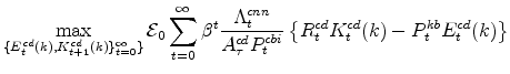
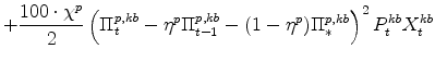
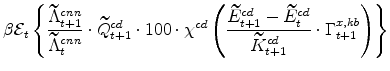
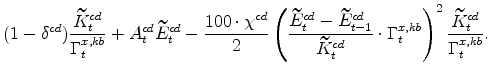
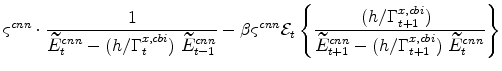
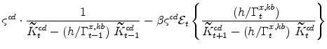
The symmetric and stationary first-order conditions implied by the consumer durables part of the capital owners'profit-maximization problem (equation 10) are:

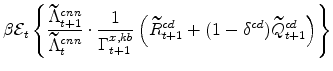
$\displaystyle \widetilde{Q}^{cd}_{t}$	$\displaystyle =$	$\displaystyle \beta \mathcal{E}_{t} \left\{\frac{% \widetilde{\Lambda}^{cnn}_{t+1}}{\widetilde{\Lambda}^{cnn}_{t}} \cdot\frac{1}{\Gamma^{x,kb}_{t+1}} \left(\widetilde{R}^{cd}_{t+1}+(1-\delta^{cd})% \widetilde{Q}^{cd}_{t+1} \right)\right\}$	(36)
$\displaystyle \widetilde{P}^{kb}_{t}$	$\displaystyle =$	$\displaystyle \widetilde{Q}^{cd}_{t} \left[% A^{cd}_{t}-100\cdot\chi^{cd} \left(\frac{\widetilde{E}^{cd}_{t} - \widetilde{E}^{cd}_{t-1}}{\widetilde{K}^{cd}_{t}}\cdot \Gamma^{x,kb}_{t}\right) \right]$
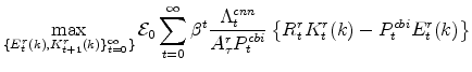
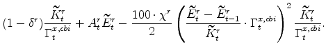
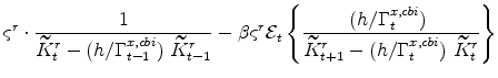
	$\displaystyle +$	$\displaystyle \beta \mathcal{E}_{t} \left\{ \frac{\widetilde{\Lambda }^{cnn}_{t+1}}{\widetilde{\Lambda}^{cnn}_{t}} \cdot \widetilde{Q}% ^{cd}_{t+1} \cdot 100 \cdot \chi^{cd} \left(\frac{\widetilde{E}% ^{cd}_{t+1} - \widetilde{E}^{cd}_{t}}{\widetilde{K}^{cd}_{t+1}}\cdot \Gamma^{x,kb}_{t+1}\right) \right\}$	(37)
$\displaystyle \widetilde{K}^{cd}_{t+1}$	$\displaystyle =$	$\displaystyle (1-\delta^{cd})\frac{\widetilde{% K}^{cd}_{t}}{\Gamma^{x,kb}_{t}} + A^{cd}_{t}\widetilde{E}^{cd}_{t} -\frac{% 100\cdot\chi^{cd}}{2} \left(\frac{\widetilde{E}^{cd}_{t} - \widetilde{E}% ^{cd}_{t-1}}{\widetilde{K}^{cd}_{t}} \cdot \Gamma^{x,kb}_{t}\right)^{2} % \frac{\widetilde{K}^{cd}_{t}}{\Gamma^{x,kb}_{t}}.$	(38)

The symmetric and stationary first-order conditions implied by the residential part of the capital owners' profit-maximization problem (equation 11) are:

$\displaystyle \widetilde{Q}^{r}_{t}$	$\displaystyle =$	$\displaystyle \beta \mathcal{E}_{t} \left\{\frac{% \widetilde{\Lambda}^{cnn}_{t+1}}{\widetilde{\Lambda}^{cnn}_{t}} \cdot\frac{1}{\Gamma^{x,cbi}_{t+1}} \left(\widetilde{R}^{r}_{t+1}+(1-\delta^{r})% \widetilde{Q}^{r}_{t+1} \right)\right\}$	(39)
$\displaystyle 1$	$\displaystyle =$	$\displaystyle \widetilde{Q}^{r}_{t} \left[A^{r}_{t}-100\cdot\chi^{r} \left(\frac{\widetilde{E}^{r}_{t} - \widetilde{E}^{r}_{t-1}}{\widetilde{K}% ^{r}_{t}}\cdot \Gamma^{x,cbi}_{t}\right) \right]$
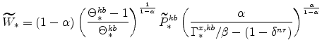
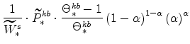
	$\displaystyle +$	$\displaystyle \beta \mathcal{E}_{t} \left\{ \frac{\widetilde{\Lambda }^{cnn}_{t+1}}{\widetilde{\Lambda}^{cnn}_{t}} \cdot \widetilde{Q}% ^{r}_{t+1} \cdot 100 \cdot \chi^{r} \left(\frac{% \widetilde{E}^{r}_{t+1} - \widetilde{E}^{r}_{t}}{\widetilde{K}^{r}_{t+1}}% \cdot \Gamma^{x,cbi}_{t+1}\right) \right\}$	(40)
$\displaystyle \widetilde{K}^{r}_{t+1}$	$\displaystyle =$	$\displaystyle (1-\delta^{r})\frac{\widetilde{K}% ^{r}_{t}}{\Gamma^{x,cbi}_{t}} + A^{r}_{t}\widetilde{E}^{r}_{t} -\frac{% 100\cdot\chi^{r}}{2} \left(\frac{\widetilde{E}^{r}_{t} - \widetilde{E}% ^{r}_{t-1}}{\widetilde{K}^{r}_{t}} \cdot \Gamma^{x,cbi}_{t}\right)^{2} % \frac{\widetilde{K}^{r}_{t}}{\Gamma^{x,cbi}_{t}}.$	(41)

The symmetric and stationary (expenditure-related) first-order conditions implied by the households' utility-maximization problem are: (equation 12) are:

$\displaystyle \widetilde{\Lambda}^{cnn}_{t}$	$\displaystyle =$	$\displaystyle \beta R_{t} \mathcal{E}% _{t}\cdot \left\{\widetilde{\Lambda}^{cnn}_{t}\cdot \frac{1}{% \Pi^{cbi}_{t+1}\Gamma^{x,cbi}_{t+1}} \right\}$	(42)
$\displaystyle \widetilde{\Lambda}^{cnn}_{t}$	$\displaystyle =$	$\displaystyle \widetilde{\Lambda}% ^{cd}_{t}\cdot\frac{1}{\widetilde{R}^{cd}_{t}}$	(43)
$\displaystyle \widetilde{\Lambda}^{cnn}_{t}$	$\displaystyle =$	$\displaystyle \widetilde{\Lambda}% ^{r}_{t}\cdot\frac{1}{\widetilde{R}^{r}_{t}}$	(44)
$\displaystyle \widetilde{\Lambda}^{cnn}_{t}$	$\displaystyle =$	$\displaystyle \varsigma^{cnn} \cdot\frac{% 1} {\widetilde{E}^{cnn}_{t}-(h/\Gamma^{x,cbi}_{t})\ \widetilde{E}^{cnn}_{t-1}} -\beta \varsigma^{cnn} \mathcal{E}_{t}\left\{% \frac{(h/\Gamma^{x,cbi}_{t+1}) \ } {\widetilde{E}% ^{cnn}_{t+1} -(h/\Gamma^{x,cbi}_{t+1})\ \widetilde{E}^{cnn}_{t}}% \right\}$	(45)
$\displaystyle \frac{\widetilde{\Lambda}^{cd}_{t}}{\Gamma^{x,kb}_{t}}$	$\displaystyle =$	$\displaystyle % \varsigma^{cd} \cdot\frac{1} {\widetilde{K}^{cd}_{t}-(h/% \Gamma^{x,kb}_{t-1})\ \widetilde{K}^{cd}_{t-1}} -\beta \varsigma^{cd} \mathcal{E}_{t}\left\{\frac{(h/\Gamma^{x,kb}_{t}) \ } {% \widetilde{K}^{cd}_{t+1}-(h/\Gamma^{x,kb}_{t})\ \widetilde{K}^{cd}_{t}}% \right\}$	(46)
$\displaystyle \frac{\widetilde{\Lambda}^{r}_{t}}{\Gamma^{x,cbi}_{t}}$	$\displaystyle =$	$\displaystyle % \varsigma^{r} \cdot\frac{1} {\widetilde{K}^{r}_{t}-(h/% \Gamma^{x,cbi}_{t-1})\ \widetilde{K}^{r}_{t-1}} -\beta \varsigma^{r} \mathcal{E}_{t}\left\{\frac{(h/\Gamma^{x,cbi}_{t})\ } {% \widetilde{K}^{r}_{t+1}-(h/\Gamma^{x,cbi}_{t})\ \widetilde{K}^{r}_{t}}% \right\}$	(47)

The key equations from the households' labor-supply decision are the wage Phillips curves

		$\displaystyle \Theta^{l}_{t}\cdot \frac{\Lambda^{l,cbi}_{t}}{\widetilde{% \Lambda}^{cnn}_{t}}\cdot L^{cbi}_{t}$
		$\displaystyle = \left(\Theta^{l}_{t}-1\right)\widetilde{W}^{cbi}_{t}L^{cbi}_{t}$
		$\displaystyle - \Theta^{l}_{t} \cdot 100\cdot\chi^{l} \left(\frac{% L^{cbi}_{\ast}}{L^{cbi}_{\ast}+L^{cbi}_{\ast}}\cdot \widetilde{W}^{cbi}_{t} +% \frac{L^{kb}_{\ast}}{L^{cbi}_{\ast}+L^{cbi}_{\ast}}\cdot \widetilde{W}% ^{kb}_{t} \right) \left(\frac{L^{cbi}_{t}}{L^{kb}_{t}} - \frac{% L^{cbi}_{t-1}}{L^{kb}_{t-1}}\right)$
		$\displaystyle + 100\cdot\chi^{w}\left(\Pi^{w,cbi}_{t} - \eta^{w}\Pi^{w,cbi}_{t-1} - (1 - \eta^{w})\Pi^{w,cbi}_{\ast}\right) \Pi^{w,cbi}_{t}\widetilde{W}% ^{cbi}_{t} L^{cbi}_{t}$
		$\displaystyle -\beta \mathcal{E}_{t} \left\{\frac{\widetilde{\Lambda}^{cnn}_{t+1}% }{\widetilde{\Lambda}^{cnn}_{t}} \cdot 100 \cdot \chi^{w} \left(\Pi^{w,cbi}_{t+1} - \eta^{w}\Pi^{w,cbi}_{t} - (1 - \eta^{w})\Pi^{w,cbi}_{\ast}\right) \Pi^{w,cbi}_{t+1}\widetilde{W}% ^{cbi}_{t+1}L^{cbi}_{t+1} \right\} \ \ \ \ \ \ \ \$	(48)
		$\displaystyle \Theta^{l}_{t}\cdot \frac{\Lambda^{l,kb}_{t}}{\widetilde{% \Lambda}^{cnn}_{t}}\cdot L^{kb}_{t}$
		$\displaystyle = \left(\Theta^{l}_{t}-1\right)\widetilde{W}^{kb}_{t}L^{kb}_{t}$
		$\displaystyle + \Theta^{l}_{t} \cdot 100\cdot\chi^{l} \left(\frac{% L^{cbi}_{\ast}}{L^{cbi}_{\ast}+L^{cbi}_{\ast}}\cdot \widetilde{W}^{cbi}_{t} +% \frac{L^{kb}_{\ast}}{L^{cbi}_{\ast}+L^{cbi}_{\ast}}\cdot \widetilde{W}% ^{kb}_{t} \right) \left(\frac{L^{cbi}_{t}}{L^{kb}_{t}} - \frac{% L^{cbi}_{t-1}}{L^{kb}_{t-1}} \right)$
		$\displaystyle + 100\cdot\chi^{w}\left(\Pi^{w,kb}_{t} - \eta^{w}\Pi^{w,kb}_{t-1} - (1 - \eta^{w})\Pi^{w,kb}_{\ast}\right) \Pi^{w,kb}_{t}\widetilde{W}% ^{kb}_{t} L^{kb}_{t}$
		$\displaystyle -\beta \mathcal{E}_{t} \left\{\frac{\widetilde{\Lambda}^{cnn}_{t+1}% }{\widetilde{\Lambda}^{cnn}_{t}} \cdot 100 \cdot \chi^{w} \left(\Pi^{w,kb}_{t+1} - \eta^{w}\Pi^{w,kb}_{t} - (1 - \eta^{w})\Pi^{w,kb}_{\ast}\right) \Pi^{w,kb}_{t+1}\widetilde{W}% ^{kb}_{t+1}L^{kb}_{t+1} \right\} \ \ \ \ \ \ \ \$	(49)

The model's other conditions for equilibrium, listed in appendix A for the non-stationary model, are transformed as follows in the stationary model:

The model's market clearing conditions become:

$\displaystyle \widetilde{X}^{cbi}_{t}=\widetilde{E}^{cnn}_{t}+\widetilde{E}^{r}_{t}+\widetilde{X}^{HG}_{t},\ \widetilde{X}^{kb}_{t}=\widetilde{E}^{cd}_{t}+\widetilde{E}^{nr}_{t}+\widetilde{X}^{HG}_{t}, \ \widetilde{K}^{u,nr,cbi}_{t}=U^{cbi}_{t}\widetilde{K}^{nr,cbi}_{t}, \ \mathrm{and} \ \widetilde{K}^{u,nr,kb}_{t}=U^{kb}_{t}\widetilde{K}% ^{nr,kb}_{t}.$
The identities between real wages, relative prices, and wage and price inflation rates become:

$\displaystyle \widetilde{P}^{kb}_{t} =\frac{\Pi^{p,kb}_{t}}{\Pi^{p,cbi}_{t}}\cdot\frac{% \Gamma^{x,kb}_{t}}{\Gamma^{x,cbi}_{t}}\cdot\widetilde{P}^{kb}_{t-1},\ \widetilde{P}^{ch}_{t} =\frac{\Pi^{p,ch}_{t}}{\Pi^{p,cbi}_{t}}\cdot \widetilde{P}^{kb}_{t-1} \ \ \mathrm{and} \ \ \widetilde{W}^{s}_{t} =\frac{% \Pi^{w,s}_{t}}{\Pi^{p,cbi}_{t}}\cdot\frac{1}{\Gamma^{x,cbi}_{t}}\cdot \widetilde{W}^{s}_{t-1}\ \ {\mathrm{for}}\ s=cbi,kb$
Equations (15) and (17) that describe the behavior of monetary policy are already described in terms of stationary variables;

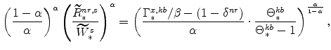
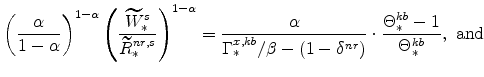
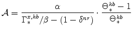
B. The Steady-state Solution to the Symmetric and Stationary Model

The steady-state growth rates in the fast- and slow-growing sectors of the economy are, respectively,

$\displaystyle \Gamma^{x,kb}_{\ast}$	$\displaystyle =$	$\displaystyle \Gamma^{z,{m}}_{\ast} \Gamma^{z,kb}_{\ast}\ \ \ \mathrm{and}$	(50)
$\displaystyle \Gamma^{x,cbi}_{\ast}$	$\displaystyle =$	$\displaystyle \Gamma^{z,{m}}_{\ast} ( \Gamma^{z,kb}_{\ast} )^{\alpha}.$	(51)

From the steady-state version of the Euler equation (equation 42), we know that the steady-state nominal interest rate is given by:

$\displaystyle R_{\ast}=\frac{1}{\beta}\cdot\Gamma^{x,cbi}_{\ast} \Pi^{p,cbi}_{\ast} =\frac{% 1}{\beta}\cdot\Gamma^{x,kb}_{\ast} \Pi^{k}_{\ast}$

(52)

while the real interest rates relevant to consumers, capital owners, and producers respectively are:

$\displaystyle \frac{R_{\ast}}{\Pi^{p,cbi}_{\ast}}$	$\displaystyle =$	$\displaystyle \frac{1}{\beta}% \cdot\Gamma^{x,cbi}_{\ast} \ \ \ \mathrm{and}$	(53)
$\displaystyle \frac{R_{\ast}}{\Pi^{p,kb}_{\ast}}$	$\displaystyle =$	$\displaystyle \frac{1}{\beta}% \cdot\Gamma^{x,kb}_{\ast} = \frac{1}{\beta}\cdot\Gamma^{x,cbi}_{\ast} \cdot\frac{\Pi^{p,cbi}_{\ast}}{\Pi^{p,kb}_{\ast}}.$	(54)

The steady-state values of the relative prices of fast-growing goods ( $% \widetilde{P}^{kb}_{t}$ ), installed non-residential capital goods ( $% \widetilde{Q}^{nr}_{t}$ ) and installed consumer durables ( $\widetilde{Q}% ^{cd}_{t}$ ) is equal to the steady-state relative mark-ups in the two sectors. Since we assume that $\Theta^{cbi}_{\ast}=\Theta^{kb}_{\ast}$ , these relative prices are all unity in the steady-state. The relative price of installed residential capital goods ( $\widetilde{Q}^{r}_{t}$ ) is also unity. Specifically,

$\displaystyle \widetilde{P}^{kb}_{\ast} =\widetilde{Q}^{cd}_{\ast} =\widetilde{Q}% ^{nr}_{\ast} =\frac{\Theta^{kb}_{\ast}}{\Theta^{kb}_{\ast}-1} \cdot \frac{\Theta^{cbi}_{\ast}-1}{\Theta^{cbi}_{\ast}}=1 \ {\mathrm{and}} \ \widetilde{Q}^{r}_{\ast}=1.$

The steady-state values of real marginal cost, the real rental rate, and the real wage can be calculated from the steady-state versions of equations (25), (26), (27), (28), (29), and (30). These are

$\displaystyle \widetilde{MC}^{cbi}_{\ast}$	$\displaystyle =$	$\displaystyle \widetilde{MC}^{kb}_{\ast}=% \frac{\Theta^{cbi}_{\ast}-1}{\Theta^{cbi}_{\ast}}, =\widetilde{P}% ^{kb}_{\ast}\cdot\frac{\Theta^{kb}_{\ast}-1}{\Theta^{kb}_{\ast}},$	(55)
$\displaystyle \widetilde{R}^{nr,s}_{\ast}$	$\displaystyle =$	$\displaystyle \widetilde{R}^{nr}_{\ast}= \widetilde{P}^{kb}_{\ast} \left(\frac{1}{\beta}\cdot\Gamma^{x,kb}_{\ast}-% \left(1-\delta^{nr} \right)\right) = \widetilde{P}^{kb}_{\ast} \left(% \frac{R_{\ast}}{\Pi^{p,kb}_{\ast}}-\left(1-\delta^{nr} \right) \right), \ \mathrm{and}$	(56)
$\displaystyle \widetilde{W}^{s}_{\ast}$	$\displaystyle =$	$\displaystyle \widetilde{W}_{\ast} =\left(1-\alpha \right) \left( \frac{\Theta^{kb}_{\ast}-1}{% \Theta^{kb}_{\ast}} \right)^{\frac{1}{1-\alpha}} \widetilde{P}^{kb}_{\ast} \left( \frac{\alpha}{\Gamma^{x,kb}_{\ast}/\beta -\left(1-\delta^{nr} \right)} \right)^{\frac{\alpha}{1-\alpha}}$	(57)

From our calibration of $\kappa$ , the parameter in the non-residential capital owners utilization function, we know from equation (32) that $U^{cbi}_{\ast}=U^{kb}_{\ast}=1$ . It is useful to note from the above equations that:

$\displaystyle \left(\frac{\widetilde{W}^{s}_{\ast}}{\widetilde{R}^{nr,s}_{\ast}}% \right)^{1-\alpha}$	$\displaystyle =$	$\displaystyle \frac{1}{\widetilde{R}% ^{nr,s}_{\ast}}\cdot \widetilde{P}^{k}_{\ast}\cdot\frac{\Theta^{kb}_{% \ast}-1}{\Theta^{kb}_{\ast}} \left(1-\alpha \right)^{1-\alpha} \left(\alpha \right)^{\alpha}$
$\displaystyle \left(\frac{\widetilde{R}^{nr,s}_{\ast}}{\widetilde{W}^{s}_{\ast}}% \right)^{\alpha}$	$\displaystyle =$	$\displaystyle \frac{1}{\widetilde{W}^{s}_{\ast}}\cdot \widetilde{P}^{kb}_{\ast}\cdot\frac{\Theta^{kb}_{\ast}-1}{% \Theta^{kb}_{\ast}} \left(1-\alpha \right)^{1-\alpha} \left(\alpha \right)^{\alpha}$

From equations (36) and (39) note also that:

$\displaystyle \widetilde{R}^{cd}_{\ast}$	$\displaystyle =$	$\displaystyle \widetilde{P}^{kb}_{\ast} \left(\frac{1}{\beta}\cdot\Gamma^{x,kb}_{\ast}-\left(1-\delta^{cd} \right)\right) = \widetilde{P}^{kb}_{\ast} \left(\frac{R_{\ast}}{% \Pi^{p,kb}_{\ast}}-\left(1-\delta^{cd} \right) \right), \ \mathrm{and}$	(58)
$\displaystyle \widetilde{R}^{r}_{\ast}$	$\displaystyle =$	$\displaystyle \left(\frac{1}{\beta}% \cdot\Gamma^{x,cbi}_{\ast}-\left(1-\delta^{r} \right)\right) = \left(% \frac{R_{\ast}}{\Pi^{p,cbi}_{\ast}}-\left(1-\delta^{r} \right) \right)$	(59)

The steady-state inflation rates of capital prices and of nominal wages are given by:

$\displaystyle \Pi^{p,kb}_{\ast}$	$\displaystyle =$	$\displaystyle \Pi^{p,cbi}_{\ast}(\Gamma^{x,cbi}_{\ast}/\Gamma^{x,kb}_{% \ast}) = \Pi^{p,cbi}_{\ast}( 1/\Gamma^{z,kb}_{\ast} )^{1-\alpha},\ \mathrm{and}$	(60)
$\displaystyle \Pi^{w,{s}}_{\ast}$	$\displaystyle =$	$\displaystyle \Pi^{w}_{\ast} =\Pi^{p,cbi}_{\ast} \Gamma^{x,cbi}_{\ast} =\Pi^{p,cbi}_{\ast} \Gamma^{z,m}_{\ast} (\Gamma^{z,kb}_{\ast} )^{\alpha} , \ \ \mathrm{for} \ s=cbi,kb,$	(61)

where the steady-state inflation rate of consumption prices $% \Pi^{p,cbi}_{\ast}$ is set by the preferences of the central bank.

The steady-state ratios $L^{cbi}_{\ast}/\widetilde{Y}^{cbi}_{\ast}$ , $% \widetilde{K}^{nr,cbi}_{\ast}/\widetilde{X}^{cbi}_{\ast}$ , $L^{kb}_{\ast}/% \widetilde{Y}^{kb}_{\ast}$ , and $\widetilde{K}^{nr,kb}_{\ast}/\widetilde{X}% ^{kb}_{\ast}$ , which are calculated from the factor demand schedules (equations 25 and 26), are

$\displaystyle \frac{\widetilde{K}^{nr,cbi}_{\ast}}{\widetilde{X}^{cbi}_{\ast}}\cdot \frac{1}{\Gamma^{x,kb}_{\ast}}$	$\displaystyle =$	$\displaystyle \left(\frac{\alpha}{1-\alpha}% \right)^{1-\alpha} \left(\frac{\widetilde{W}^{s}_{\ast}}{\widetilde{R}% ^{nr,s}_{\ast}}\right)^{1-\alpha} =\frac{\alpha}{\Gamma^{x,kb}_{\ast}/% \beta-(1-\delta^{nr})} \cdot \frac{\Theta^{kb}_{\ast}-1}{% \Theta^{kb}_{\ast}},$	(62)
$\displaystyle \frac{L^{cbi}_{\ast}}{\widetilde{X}^{cbi}_{\ast}}$	$\displaystyle =$	$\displaystyle \left(% \frac{1-\alpha}{\alpha}\right)^{\alpha} \left(\frac{\widetilde{R}% ^{nr,s}_{\ast}}{\widetilde{W}^{s}_{\ast}}\right)^{\alpha} =\left(\frac{% \Gamma^{x,kb}_{\ast}/\beta-(1-\delta^{nr})} {\alpha} \cdot \frac{% \Theta^{kb}_{\ast}}{\Theta^{kb}_{\ast}-1} \right)^{\frac{\alpha}{1-\alpha }},$	(63)
$\displaystyle \frac{\widetilde{K}^{nr,kb}_{\ast}}{\widetilde{X}^{kb}_{\ast}}\cdot \frac{1}{% \Gamma^{x,kb}_{\ast}}$	$\displaystyle =$	$\displaystyle \left(\frac{\alpha}{1-\alpha}% \right)^{1-\alpha} \left(\frac{\widetilde{W}^{s}_{\ast}}{\widetilde{R}% ^{nr,s}_{\ast}}\right)^{1-\alpha} =\frac{\alpha}{\Gamma^{x,kb}_{\ast}/% \beta-(1-\delta^{nr})} \cdot \frac{\Theta^{kb}_{\ast}-1}{% \Theta^{kb}_{\ast}}, \ \mathrm{and} \ \ \ \ \ \ \$	(64)
$\displaystyle \frac{L^{kb}_{\ast}}{\widetilde{X}^{kb}_{\ast}}$	$\displaystyle =$	$\displaystyle \left(% \frac{1-\alpha}{\alpha}\right)^{\alpha} \left(\frac{\widetilde{R}% ^{nr,s}_{\ast}}{\widetilde{W}^{s}_{\ast}}\right)^{\alpha} =\left(\frac{% \Gamma^{x,kb}_{\ast}/\beta-(1-\delta^{nr})} {\alpha} \cdot \frac{% \Theta^{kb}_{\ast}}{\Theta^{kb}_{\ast}-1} \right)^{\frac{\alpha}{1-\alpha }}.$	(65)

We can write these as

$\displaystyle \frac{\widetilde{K}^{nr,cbi}_{\ast}}{\widetilde{X}^{cbi}_{\ast}}\cdot\frac{1}{\Gamma^{x,kb}_{\ast}} =\mathcal{A}, \ \ \ \ \frac{\widetilde{L}% ^{cbi}_{\ast}}{\widetilde{X}^{cbi}_{\ast}}=(\mathcal{A})^{-\frac{\alpha}{% 1-\alpha}}, \ \ \ \ \frac{\widetilde{K}^{nr,kb}_{\ast}}{\widetilde{X}% ^{kb}_{\ast}}\cdot\frac{1}{\Gamma^{x,kb}_{\ast}} =\mathcal{A}, \ \ \ \ {% \mathrm{and}}\ \ \ \ \frac{\widetilde{L}^{kb}_{\ast}}{\widetilde{X}% ^{kb}_{\ast}}=(\mathcal{A})^{-\frac{\alpha}{1-\alpha}},$

(66)

where

$\displaystyle {\mathcal{A}}= \frac{\alpha}{\Gamma^{x,kb}_{\ast}/\beta-(1-\delta^{nr})} \cdot \frac{\Theta^{kb}_{\ast}-1}{\Theta^{kb}_{\ast}}$

We calibrate aggregate labor input, $L_{\ast }^{cbi}+L_{\ast }^{kb}$ , to 0.25. To solve for $L_{\ast }^{cbi}$ , $\widetilde{K}_{\ast }^{cbi}$ , $% L_{\ast }^{kb}$ , and $\widetilde{K}_{\ast }^{kb}$ by themselves we need to solve first for $\widetilde{X}_{\ast }^{cbi}$ and $\widetilde{X}_{\ast }^{kb}$ . This takes a few steps. The first step is to derive the ratio of $\widetilde{X}_{\ast }^{kb}/\widetilde{X}_{\ast }^{cbi}$ ; as we have assumed that autonomous demand enters symmetrically, its presence has no effect on this steady-state ratio, so we suppress this portion of demand in the following.

As part of this exercise we must turn to considering the expenditure side of the model, and in particular the model's expenditure ratios. The normalizing factors $% \varsigma ^{cd}$ and $\varsigma^{r}$ are calibrated so that the ratios $% \frac{\widetilde{E}_{\ast }^{cd}}{\widetilde{E}_{\ast }^{cnn}}$ and $\frac{% \widetilde{E}_{\ast }^{r}}{\widetilde{E}_{\ast }^{cnn}}$ are 0.1682 and 0.2094 respectively.

To calculate the model's expenditure ratios, we start with what we know about the ratios between the inputs to the optimizing household's utility function, that is $E_{\ast }^{cnn}$ , $K_{\ast }^{cd}$ , and $K_{\ast }^{r}$ . We know from equations (43) to (47) that

$\displaystyle \frac{\widetilde{K}_{\ast }^{cd}}{\widetilde{E}_{\ast }^{cnn}}$	$\displaystyle =$	$\displaystyle \frac{\varsigma ^{cd}}{\varsigma ^{cnn}}\cdot \frac{1-\beta h/\Gamma ^{x,kb}}{1-\beta h/\Gamma ^{x,cbi}}\cdot \frac{% 1-h/\Gamma ^{x,cbi}}{1-h/\Gamma ^{x,kb}}\cdot \frac{1}{\widetilde{% R}_{\ast }^{cd}},\ \mathrm{and}$
$\displaystyle \frac{\widetilde{K}_{\ast }^{r}}{\widetilde{E}_{\ast }^{cnn}}$	$\displaystyle =$	$\displaystyle \frac{\varsigma ^{r}}{\varsigma ^{cnn}}\cdot \frac{1-\beta h/\Gamma ^{x,cbi}}{1-\beta h/\Gamma ^{x,cbi}}\cdot \frac{% 1-h/\Gamma ^{x,cbi}}{1-h/\Gamma ^{x,cbi}}\cdot \frac{1}{\widetilde{% R}_{\ast }^{r}}$

We have expressions for $\widetilde{R}_{\ast }^{cd}$ and $\widetilde{R}% _{\ast }^{r}$ in equations (58) and (59) and we know from the steady-state versions of equations (38) and (41) that

$\displaystyle \frac{\widetilde{E}_{\ast }^{cd}}{\widetilde{K}_{\ast }^{cd}}=\left( \frac{% \Gamma _{\ast }^{x,kb}-(1-\delta ^{cd})}{\Gamma _{\ast }^{x,kb}}\right) \ \ \ \mathrm{and}\ \ \ \ \frac{\widetilde{E}_{\ast }^{r}}{\widetilde{K}_{\ast }^{r}}=\left( \frac{\Gamma _{\ast }^{x,cbi}-(1-\delta ^{r})}{\Gamma _{\ast }^{x,cbi}}\right).$

(67)

These equations imply that the ratios of expenditures implied by the optimizing agents of the model are

$\displaystyle \frac{\widetilde{E}_{\ast }^{cd}}{\widetilde{E}_{\ast }^{cnn}}$	$\displaystyle =$	$\displaystyle \frac{\varsigma ^{cd}}{\varsigma ^{cnn}}\cdot \frac{1 - \beta h/\Gamma ^{x,kb}}{1 - \beta h/\Gamma ^{x,cbi}}\cdot \frac{% 1 - h/\Gamma ^{x,cbi}}{1 -h/\Gamma ^{x,kb}}\cdot \frac{% \Gamma _{\ast }^{x,kb} - (1 - \delta ^{cd})}{\Gamma _{\ast }^{x,kb}}% \cdot \frac{1}{\widetilde{P}_{\ast }^{kb}}\cdot \frac{\beta }{\Gamma _{\ast }^{x,kb} - \beta (1 - \delta ^{cd})} = \mathcal{D}$
			(68)
$\displaystyle \frac{\widetilde{E}_{\ast }^{r}}{\widetilde{E}_{\ast }^{cnn}}$	$\displaystyle =$	$\displaystyle \frac{\varsigma ^{r}}{\varsigma ^{cnn}}\cdot \frac{1 - \beta h/\Gamma ^{x,cbi}}{1 - \beta h/\Gamma ^{x,cbi}}\cdot \frac{% 1 - h/\Gamma ^{x,cbi}}{1 - h/\Gamma ^{x,cbi}}\cdot \frac{% \Gamma _{\ast }^{x,cbi} - (1 - \delta ^{r})}{\Gamma _{\ast }^{x,cbi}}% \cdot \frac{\beta }{\Gamma _{\ast }^{x,cbi} - \beta (1 - \delta ^{r})}% = \mathcal{R}\ \ \ \ \ \ \ \$	(69)

We can now consider expenditures as shares of their sector's outputs. Recall from the equilibrium conditions listed in appendix A that

$\displaystyle E_{\ast }^{cnn}+E_{\ast }^{r} = X_{\ast }^{cbi}\ \ \mathrm{and}\ \ E_{\ast }^{cd}+E_{\ast }^{nr} = X_{\ast }^{kb},$

Consider first the market clearing condition for the slow growing sector. Since all aggregates in this equation grow at the same rate we can re-write the steady-state expression for $X_{t}^{cbi}$ as shown below (as well as in appendix B) and with some manipulations

$\displaystyle \widetilde{X}_{\ast }^{cbi}$	$\displaystyle =$	$\displaystyle \widetilde{E}_{\ast }^{cnn}+% \widetilde{E}_{\ast }^{r}\ \mathrm{implies}$
$\displaystyle 1$	$\displaystyle =$	$\displaystyle \frac{\widetilde{E}_{\ast }^{cnn}}{\widetilde{X}_{\ast }^{cbi}}+\frac{\widetilde{E}_{\ast }^{r}}{\widetilde{X}_{\ast }^{cbi}}\ =\ \frac{\widetilde{E}_{\ast }^{cnn}}{\widetilde{X}_{\ast }^{cbi}}+\frac{% \widetilde{E}_{\ast }^{r}}{\widetilde{E}_{\ast }^{cnn}}\cdot \frac{% \widetilde{E}_{\ast }^{cnn}}{\widetilde{X}_{\ast }^{cbi}}\ =\ \frac{% \widetilde{E}_{\ast }^{cnn}}{\widetilde{X}_{\ast }^{cbi}}\left( 1+\frac{% \widetilde{E}_{\ast }^{r}}{\widetilde{E}_{\ast }^{cnn}}\right) \ =\ \frac{% \widetilde{E}_{\ast }^{cnn}}{\widetilde{X}_{\ast }^{cbi}}\left( 1+\mathcal{R}% \right).$

This then allows us to write:

$\displaystyle \frac{\widetilde{E}_{\ast }^{cnn}}{\widetilde{X}_{\ast }^{cbi}} = \frac{% \widetilde{E}_{\ast }^{cnn}}{\widetilde{E}_{\ast }^{cnn} + \widetilde{E}% _{\ast }^{r}} = \frac{1}{1 + \widetilde{E}_{\ast }^{r}/\widetilde{E}% _{\ast }^{cnn}} = \frac{1}{1 + \mathcal{R}}\ \ \mathrm{and}\ \ \frac{% \widetilde{E}_{\ast }^{r}}{\widetilde{X}_{\ast }^{cbi}} = 1 - \frac{% \widetilde{E}_{\ast }^{cnn}}{\widetilde{X}_{\ast }^{cbi}} = 1 - \frac{1}{% 1 + \mathcal{R}} = \frac{\mathcal{R}}{1 + \mathcal{R}},$

(70)

where $\mathcal{R}$ was defined in equation (69). For the fast-growing sector, we can re-write the market clearing condition (as in appendix B) as:

$\displaystyle \widetilde{X}_{\ast }^{kb} = \widetilde{E}_{\ast }^{cd}+\widetilde{E}% _{\ast }^{nr}.$

and make similar tranformations as before. A useful relationship for these transformations is from equations (34) and (35), that is,

$\displaystyle \widetilde{E}_{\ast }^{nr}=\left( \frac{\Gamma _{\ast }^{x,kb}-(1-\delta ^{nr})}{\Gamma _{\ast }^{x,kb}}\right) \widetilde{K}_{\ast }^{nr}=\left( \frac{\Gamma _{\ast }^{x,kb}-(1-\delta ^{nr})}{\Gamma _{\ast }^{x,kb}}% \right) \left( \widetilde{K}_{\ast }^{nr,cbi}+\widetilde{K}_{\ast }^{nr,kb}\right).$

The fast growing sector's market clearing condition can also be manipulated; specifically,

$\displaystyle \widetilde{X}_{\ast }^{kb}$	$\displaystyle =$	$\displaystyle \widetilde{E}_{\ast }^{cd}+% \widetilde{E}_{\ast }^{nr}\ \mathrm{implies}$
$\displaystyle 1$	$\displaystyle =$	$\displaystyle \frac{\widetilde{E}_{\ast }^{cd}}{\widetilde{X}_{\ast }^{kb}}+\fr... ...b}} + % \frac{\widetilde{K}_{\ast }^{nr,kb}}{\widetilde{X}_{\ast }^{kb}}\right)$

We have expressions for $\frac{\widetilde{E}_{\ast }^{cd}}{\widetilde{E}% _{\ast }^{cnn}}$ , $\frac{\widetilde{E}_{\ast }^{cnn}}{\widetilde{X}_{\ast }^{cbi}}$ , $\frac{\widetilde{K}_{\ast }^{nr,cbi}}{\widetilde{X}_{\ast }^{cbi}% }$ , and $\frac{\widetilde{K}_{\ast }^{nr,kb}}{\widetilde{X}_{\ast }^{kb}}$ . Substituting in these expressions yields

$\displaystyle 1 = \mathcal{D}\left( \frac{1}{1+\mathcal{R}}\right) \cdot \frac{\widetilde{X}_{\ast }^{cbi}}{\widetilde{X}_{\ast }^{kb}}+\left( \frac{% \Gamma _{\ast }^{x,kb}-(1-\delta ^{nr})}{\Gamma _{\ast }^{x,kb}}\right) \mathcal{A}\cdot \Gamma _{\ast }^{x,kb}\left( \frac{\widetilde{X}_{\ast }^{cbi}}{\widetilde{X}_{\ast }^{kb}}+1\right) ,$

which can be re-arranged to

$\displaystyle \frac{\widetilde{X}_{\ast }^{kb}}{\widetilde{X}_{\ast }^{cbi}}=\frac{% \mathcal{D}+\left( 1+\mathcal{R}\right) \left( \Gamma _{\ast }^{x,kb}-(1-\delta ^{nr})\right) \mathcal{A}}{\left( 1+\mathcal{R}\right) -\left( 1+\mathcal{R}\right) \left( \Gamma _{\ast }^{x,kb}-(1-\delta ^{nr})\right) \mathcal{A}}=\mathcal{B}.$

(71)

This then allows us to write:

$\displaystyle \frac{\widetilde{E}_{\ast }^{nr}}{\widetilde{X}_{\ast }^{kb}}=\left( \frac{% \Gamma _{\ast }^{x,kb} - (1 - \delta ^{nr})}{\Gamma _{\ast }^{x,kb}}% \right) \left( \frac{\widetilde{K}_{\ast }^{nr,cbi}}{\widetilde{X}_{\ast }^{cbi}}\cdot \frac{\widetilde{X}_{\ast }^{cbi}}{\widetilde{X}_{\ast }^{kb}}% + \frac{\widetilde{K}_{\ast }^{nr,kb}}{\widetilde{X}_{\ast }^{kb}}\right) =\left( \frac{\Gamma _{\ast }^{x,kb} - (1 - \delta ^{nr})}{\Gamma _{\ast }^{x,kb}}\right) \mathcal{A}\cdot \frac{1 + \mathcal{B}}{\mathcal{B}},$

(72)

so that

$\displaystyle \frac{\widetilde{E}_{\ast }^{cd}}{\widetilde{X}_{\ast }^{kb}}=1-\frac{% \widetilde{E}_{\ast }^{nr}}{\widetilde{X}_{\ast }^{kb}}=1-\left( \frac{% \Gamma _{\ast }^{x,kb} - (1 - \delta ^{nr})}{\Gamma _{\ast }^{x,kb}}% \right) \mathcal{A}\cdot \frac{1 + \mathcal{B}}{\mathcal{B}}.$

Since the right-hand sides of equations (63) and (65) are identical, $\widetilde{L}_{\ast }^{cbi}/\widetilde{X}_{\ast }^{cbi}=% \widetilde{L}_{\ast }^{kb}/\widetilde{X}_{\ast }^{kb}$ . As a result, $% \widetilde{X}_{\ast }^{kb}/\widetilde{X}_{\ast }^{cbi}=\mathcal{B}$ implies that $L_{\ast }^{kb}/L_{\ast }^{cbi}=\mathcal{B}$ , which means then that:

$\displaystyle L_{\ast }^{cbi}=\frac{1}{1+\mathcal{B}}\cdot \mathcal{L}\ \ \ \mathrm{and}\ \ \ L_{\ast }^{kb}=\frac{\mathcal{B}}{1+\mathcal{B}}\cdot \mathcal{L}.$

where $\mathcal{L}=L_{\ast }^{cbi}+L_{\ast }^{kb}$ is 0.25. Solving for $% L_{\ast }^{cbi}$ and $L_{\ast }^{kb}$ allows us to find the steady-state solutions for all of the other production, factor, and expenditure variables of the model. Specifically:

$L^{cbi}_{\ast}$ and $L^{cbi}_{\ast}/\widetilde{X}% ^{cbi}_{\ast}$ (defined in equation 63) imply $\widetilde{X}% ^{cbi}_{\ast}$ ;
$L^{kb}_{\ast}$ and $L^{kb}_{\ast}/\widetilde{X}% ^{kb}_{\ast}$ (defined in equation 65) imply $\widetilde{X}% ^{kb}_{\ast}$ ;
$\widetilde{X}^{cbi}_{\ast}$ and $\widetilde{K}% ^{nr,cbi}_{\ast}/\widetilde{X}^{cbi}_{\ast}$ (defined in equation 62) imply $\widetilde{K}^{nr,cbi}_{\ast}$ and (since $U^{cbi}_{\ast}=1$ ) $\widetilde{K}^{u,nr,cbi}_{\ast}$ ;
$\widetilde{X}^{kb}_{\ast}$ and $\widetilde{K}% ^{nr,kb}_{\ast}/\widetilde{X}^{kb}_{\ast}$ (defined in equation 64) imply $\widetilde{K}^{nr,kb}_{\ast}$ and (since $U^{kb}_{\ast}=1$ ) $% \widetilde{K}^{u,nr,kb}_{\ast}$ ;
$\widetilde{K}^{nr,cbi}_{\ast}$ , $\widetilde{K}% ^{nr,kb}_{\ast}$ , and the non-residential capital market clearing condition imply $\widetilde{K}^{nr}_{\ast}$ ;
$\widetilde{X}^{cbi}_{\ast}$ and $\widetilde{E}% ^{cnn}_{\ast}/\widetilde{X}^{cbi}_{\ast}$ and $\widetilde{E}^{r}_{\ast}/% \widetilde{X}^{cbi}_{\ast}$ (both defined in equation 70) imply $\widetilde{E}^{cnn}_{\ast}$ and $\widetilde{E}^{r}_{\ast}$ ;
$\widetilde{X}^{kb}_{\ast}$ and $\widetilde{E}% ^{cd}_{\ast}/\widetilde{X}^{kb}_{\ast}$ and $\widetilde{E}^{nr}_{\ast}/% \widetilde{X}^{kb}_{\ast}$ (defined in equations 72 and B) imply $\widetilde{E}^{cd}_{\ast}$ and $\widetilde{E}^{nr}_{\ast}$ ;
$\widetilde{E}^{cd}_{\ast}$ and $\widetilde{E}% ^{r}_{\ast}$ , and $\widetilde{E}^{cd}_{\ast}/\widetilde{K}^{cd}_{\ast}$ and $% \widetilde{E}^{r}_{\ast}/\widetilde{K}^{r}_{\ast}$ (both defined in equation 67) imply $\widetilde{K}^{cd}_{\ast}$ and $\widetilde{K}^{r}_{\ast}$ ; and,
$\widetilde{\Lambda}^{cnn}_{\ast}$ , $\widetilde{% \Lambda}^{cd}_{\ast}$ , and $\widetilde{\Lambda}^{r}_{\ast}$ are then implied by the steady-state versions of equations (45) to (47).

The reader can verify that we have in this section presented a steady-state value for all of the model variables that defined equilibrium in appendix A.

C. List of Model Parameters

Habit-persistence parameter for the consumption of non-durable goods and non-housing services.

$\alpha=$ The elasticity of output with respect to capital.

$\beta=$ The household's discount factor.

$\delta^{cd}=$ The quarterly depreciation rate of consumer durables.

$\delta^{nr}=$ The quarterly depreciation rate of non-residential capital.

$\delta^{r}=$ The quarterly depreciation rate of residential capital.

$\eta^{p}=$ Parameter reflecting the relative importance of lagged price inflation in the adjustment cost function for prices.

$\eta^{w}=$ Parameter reflecting the relative importance of lagged wage inflation in the adjustment cost function for wages.

$\kappa=$ Variable capacity utilization scaling parameter.

$\nu=$ Inverse labor supply elasticity.

$\rho^{a,nr}=$ Persistence parameter in the AR(1) process describing the evolution of $A^{nr}_{t}$ .

$\rho^{a,cd}=$ Persistence parameter in the AR(1) process describing the evolution of $A^{cd}_{t}$ .

$\rho^{a,r}=$ Persistence parameter in the AR(1) process describing the evolution of $A^{r}_{t}$ .

$\rho^{\omega}=$ Persistence parameter in the AR(1) process describing the evolution of $\Omega_{t}$ .

$\varsigma^{cnn}=$ Co-efficient on the consumer non-durable goods and non-housing serives component of the utility function.

$\varsigma^{cd}=$ Co-efficient on the consumer durable goods component of the utility function.

$\varsigma^{r}=$ Co-efficient on the consumer housing serives component of the utility function.

$\varsigma^{l}=$ Co-efficient on the labor supply components of the utility function.

$\phi^{Y}=$ Co-efficient on GDP gap in the monetary policy reaction function.

$\phi^{\Delta Y}=$ Co-efficient on change in the GDP gap in the monetary policy reaction function.

$\phi^{\pi}=$ Co-efficient on GDP price inflation in the monetary policy reaction function.

$\phi^{r}=$ Co-efficient on lagged nominal interest rates in the monetary policy reaction function.

$\chi^{cd}=$ Investment adjustment costs in the consumer durables evolution equation.

$\chi^{nr}=$ Investment adjustment costs in the non-residential capital evolution equation.

$\chi^{r}=$ Investment adjustment costs in the residential capital evolution equation.

$\chi^{l}=$ Parameter reflecting the size of adjustment costs in the labor sectoral adjustment cost function.

$\chi^{p}=$ Parameter reflecting the size of adjustment costs in re-setting prices.

$\chi^{w}=$ Parameter reflecting the size of adjustment costs in re-setting wages.

$\psi=$ Elasticity of utilization costs.

D. List of Endogenous and Exogenous Model Variables

$\Omega_{t}=$ Aggregate risk premium.

$A^{nr}_{t}=$ Non-residential sector risk premium.

$A^{r}_{t}=$ Residential sector risk premium.

$A^{cd}_{t}=$ Consumer durables sector risk premium.

$E^{nr}_{t}=$ Expenditures on goods in the fast-growing "capital" goods sector for use in non-residential investment.

$E^{r}_{t}=$ Expenditures on goods in the slow-growing "consumption" goods sector for use in residential investment.

$E^{cd}_{t}=$ Expenditures on goods in the fast-growing "capital" goods sector for use in consumer durables investment.

$E^{cnn}_{t}=$ Expenditures on goods in the slow-growing "consumption" goods sector for use in consumer non-durable goods and non-housing services.

$\widetilde{X}^{HG}_{t}=$ Exogenous expenditure (by the government and foreign sector).

$H^{gdp}_{t}=$ Growth rate of real (chain-weighted) GDP.

$K^{u,nr,cbi}_{t}=$ The amount of utilized non-residential capital used in the slow-growing "consumption"goods sector.

$K^{u,nr,kb}_{t}=$ The amount of utilized non-residential capital used in the fast-growing "capital" goods sector.

$K^{nr,cbi}_{t}=$ The physical amount of non-residential capital used in the slow-growing "consumption" goods sector.

$K^{nr,kb}_{t}=$ The physical amount of non-residential capital used in the fast-growing "capital" goods sector.

$K^{nr}_{t}=$ The aggregate non-residential capital stock.

$K^{r}_{t}=$ The residential capital stock.

$K^{cd}_{t}=$ The consumer durables capital stock.

$L^{cbi}_{t}=$ Labor used in the slow-growing "consumption" goods sector.

$L^{kb}_{t}=$ Labor used in the fast-growing "capital" goods sector.

$MC^{cbi}_{t}=$ Marginal cost in the slow-growing "consumption" goods sector.

$MC^{kb}_{t}=$ Marginal cost in the fast-growing "capital" goods sector.

$P^{cbi}_{t}=$ Price level in the slow-growing "consumption" goods sector.

$P^{kb}_{t}=$ Price level in the fast-growing "capital" goods sector.

$Q^{nr}_{t}=$ Price of installed non-residential capital.

$Q^{r}_{t}=$ Price of installed residential capital.

$Q^{cd}_{t}=$ Price of installed consumer durables capital.

$R_{t}=$ Nominal interest rate.

$R^{nr,cbi}_{t}=$ The nominal rental rate on non-residential capital used in the slow-growing "consumption" goods sector.

$R^{nr,kb}_{t}=$ The nominal rental rate on non-residential capital used in the fast-growing "capital" goods sector.

$R^{nr}_{t}=$ The aggregate nominal rental rate on non-residential capital.

$R^{r}_{t}=$ The nominal rental rate on residential capital.

$R^{cd}_{t}=$ The nominal rental rate on consumer durables capital.

$U^{cbi}_{t}=$ The utilization rate of non-residential capital used in the slow-growing "consumption" goods sector.

$U^{kb}_{t}=$ The utilization rate of non-residential capital used in the fast-growing "capital" goods sector.

$W^{cbi}_{t}=$ The nominal wage in the slow-growing "consumption" goods sector.

$W^{kb}_{t}=$ The nominal wage in the fast-growing "capital" goods sector.

$X^{cbi}_{t}=$ Production in the slow-growing "consumption" goods sector.

$X^{kb}_{t}=$ Production in the fast-growing "capital" goods sector.

$(Z^{kb}_{t})^{1-\alpha}=$ Level of capital-specific technology.

$(Z^{m}_{t})^{1-\alpha}=$ Level of economy-wide technology.

$\Gamma^{x,cbi}_{t}=$ Growth rate of output in the consumption (slow growth) sector consistent with the growth rate of technology. (Note $% \Gamma^{x,cbi}_{t}$ is not in general equal to $% \ln(X^{cbi}_{t}/X^{cbi}_{t-1})$ . Rather it is equal to $\Gamma^{z,m}_{t}(% \Gamma^{z,kb}_{t})^\alpha$ .)

$\Gamma^{x,kb}_{t}=$ Growth rate of output in the consumption (slow growth) sector consistent with the growth rate of technology. (Note $% \Gamma^{x,kb}_{t}$ is not in general equal to $% \ln(X^{kb}_{t}/X^{kb}_{t-1})$ . Rather it is equal to $\Gamma^{z,m}_{t}% \Gamma^{z,kb}_{t}$ .)

$(1-\alpha)\Gamma^{z,kb}_{t}=$ The growth rate of the level of capital-specific technology.

$(1-\alpha)\Gamma^{z,m}_{t}=$ The growth rate of the level of economy-wide technology.

$\Theta^{l}_{t}=$ The elasticity of subsitution between the differentiated labor inputs into production.

$\Theta^{cbi}_{t}=$ The elasticity of subsitution between the differentiated intermediate inputs in the slow-growing "consumption" goods sector.

$\Theta^{kb}_{t}=$ The elasticity of subsitution between the differentiated intermediate inputs in the fast-growing "capital" goods sector.

$\Lambda^{r}_{t}=$ The marginal utility of residential capital.

$\Lambda^{cd}_{t}=$ The marginal utility of durable goods.

$\Lambda^{cnn}_{t}=$ The marginal utility of non-durable goods and non-housing services consumption.

$\Lambda^{l,cbi}_{t}=$ The marginal dis-utility of supplying labor in the slow-growing "consumption" goods sector.

$\Lambda^{l,kb}_{t}=$ The marginal dis-utility of supplying labor in the fast-growing "capital" goods sector.

$\Pi^{c}_{t}=$ The inflation rate of the PCE deflator.

$\Pi^{p,cbi}_{t}=$ The inflation rate for prices in the slow-growing "consumption" goods sector.

$\Pi^{p,kb}_{t}=$ The inflation rate for prices in the fast-growing "capital" goods sector.

$\Pi^{w,cbi}_{t}=$ The inflation rate of nominal wages in the slow-growing "consumption" goods sector.

$\Pi^{w,kb}_{t}=$ The inflation rate of nominal wages in the fast-growing "capital" goods sector.

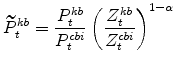
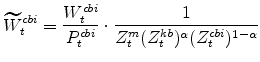
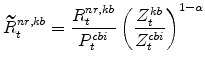
E. Definitions of Stationary Model Variables

In this section we provide definitions for all of the variables of the model that must be transformed in order to render them stationary. Note that in going through our list of model variables we leave out those that are already stationary.

The model's output variables in stationary form are:

		$\displaystyle \widetilde{X}^{cbi}_{t} =\frac{X^{cbi}_{t}}{Z^{m}_{t}(Z^{kb}_{t})^{% \alpha}(Z^{cbi}_{t})^{1-\alpha}}$
		$\displaystyle \widetilde{X}^{kb}_{t}=\frac{X^{kb}_{t}}{Z^{m}_{t}Z^{kb}_{t}}$

The model's expenditure variables in stationary form are:

		$\displaystyle \widetilde{E}^{nr}_{t} =\frac{E^{nr}_{t}}{Z^{m}_{t}Z^{kb}_{t}}$
		$\displaystyle \widetilde{E}^{r}_{t} =\frac{E^{r}_{t}}{Z^{m}_{t}(Z^{kb}_{t})^{% \alpha}(Z^{cbi}_{t})^{1-\alpha}}$
		$\displaystyle \widetilde{E}^{cd}_{t} =\frac{E^{cd}_{t}}{Z^{m}_{t}Z^{kb}_{t}}$
		$\displaystyle \widetilde{E}^{cnn}_{t}=\frac{E^{cc}_{t}}{Z^{m}_{t}(Z^{kb}_{t})^{% \alpha}(Z^{cbi}_{t})^{1-\alpha}}$

The model's marginal utility variables in stationary form are:

		$\displaystyle \widetilde{\Lambda}^{r}_{t} =\Lambda^{r}_{t}Z^{m}_{t}(Z^{kb}_{t})^{\alpha}(Z^{cbi}_{t})^{1-\alpha}$
		$\displaystyle \widetilde{\Lambda}^{cd}_{t} =\Lambda^{cd}_{t}Z^{m}_{t}Z^{kb}_{t}$
		$\displaystyle \widetilde{\Lambda}^{cnn}_{t} =\Lambda^{cnn}_{t}Z^{m}_{t}(Z^{kb}_{t})^{\alpha}(Z^{cbi}_{t})^{1-\alpha}$

The model's capital stock variables in stationary form are:

		$\displaystyle \widetilde{K}^{u,nr,cbi}_{t}=\frac{K^{u,nr,cbi}_{t}}{Z^{m}_{t}Z^{kb}_{t}}$
		$\displaystyle \widetilde{K}^{u,nr,kb}_{t}=\frac{K^{u,nr,kb}_{t}}{Z^{m}_{t}Z^{kb}_{t}}$
		$\displaystyle \widetilde{K}^{nr,cbi}_{t}=\frac{K^{nr,cbi}_{t}}{Z^{m}_{t}Z^{kb}_{t}}$
		$\displaystyle \widetilde{K}^{nr,kb}_{t}=\frac{K^{nr,kb}_{t}}{Z^{m}_{t}Z^{kb}_{t}}$
		$\displaystyle \widetilde{K}^{nr}_{t+1}=\frac{K^{nr}_{t}}{Z^{m}_{t}Z^{kb}_{t}}$
		$\displaystyle \widetilde{K}^{r}_{t+1}=\frac{K^{r}_{t}}{Z^{m}_{t}(Z^{kb}_{t})^{% \alpha}(Z^{cbi}_{t})^{1-\alpha}}$
		$\displaystyle \widetilde{K}^{cd}_{t+1}=\frac{K^{cd}_{t}}{Z^{m}_{t}Z^{kb}_{t}}$

The model's relative (KB) output price variable in stationary form is:

$\displaystyle \widetilde{P}^{kb}_{t}=\frac{P^{kb}_{t}}{P^{cbi}_{t}} \left(\frac{Z^{kb}_{t}% }{Z^{cbi}_{t}}\right)^{1-\alpha}$

The model's real wage variables are:

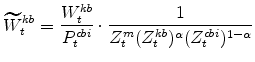		$\displaystyle \widetilde{W}^{cbi}_{t}=\frac{W^{cbi}_{t}}{P^{cbi}_{t}} \cdot \frac{1}{% Z^{m}_{t}(Z^{kb}_{t})^{\alpha}(Z^{cbi}_{t})^{1-\alpha}}$
		$\displaystyle \widetilde{W}^{kb}_{t}=\frac{W^{kb}_{t}}{P^{cbi}_{t}} \cdot \frac{1}{% Z^{m}_{t}(Z^{kb}_{t})^{\alpha}(Z^{cbi}_{t})^{1-\alpha}}$

The model's real rental rate variables in stationary form are:

		$\displaystyle \widetilde{R}^{nr,cbi}_{t}=\frac{R^{nr,cbi}_{t}}{P^{cbi}_{t}}\left(\frac{% Z^{kb}_{t}}{Z^{cbi}_{t}}\right)^{1-\alpha}$
		$\displaystyle \widetilde{R}^{nr,kb}_{t}=\frac{R^{nr,kb}_{t}}{P^{cbi}_{t}}\left(\frac{% Z^{kb}_{t}}{Z^{cbi}_{t}}\right)^{1-\alpha}$
		$\displaystyle \widetilde{R}^{nr}_{t}=\frac{R^{nr}_{t}}{P^{cbi}_{t}}\left(\frac{Z^{kb}_{t}% }{Z^{cbi}_{t}}\right)^{1-\alpha}$
		$\displaystyle \widetilde{R}^{r}_{t}=\frac{R^{r}_{t}}{P^{cbi}_{t}}$
		$\displaystyle \widetilde{R}^{cd}_{t}=\frac{R^{cd}_{t}}{P^{cbi}_{t}} \left(\frac{% Z^{kb}_{t}}{Z^{cbi}_{t}}\right)^{1-\alpha}$

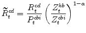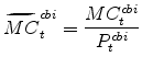
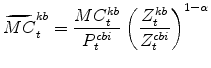
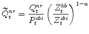
The model's real marginal cost variables in stationary form are:

		$\displaystyle \widetilde{MC}^{cbi}_{t}=\frac{MC^{cbi}_{t}}{P^{cbi}_{t}}$
		$\displaystyle \widetilde{MC}^{kb}_{t}=\frac{MC^{kb}_{t}}{P^{cbi}_{t}} \left(\frac{% Z^{kb}_{t}}{Z^{cbi}_{t}}\right)^{1-\alpha}$

The model's relative price of installed capital variables in stationary form are:

		$\displaystyle \widetilde{Q}^{nr}_{t}=\frac{Q^{nr}_{t}}{P^{cbi}_{t}} \left(\frac{% Z^{kb}_{t}}{Z^{cbi}_{t}}\right)^{1-\alpha}$
		$\displaystyle \widetilde{Q}^{r}_{t}=\frac{Q^{r}_{t}}{P^{cbi}_{t}}$
		$\displaystyle \widetilde{Q}^{cd}_{t}=\frac{Q^{cd}_{t}}{P^{cbi}_{t}} \left(\frac{% Z^{kb}_{t}}{Z^{cbi}_{t}}\right)^{1-\alpha}$

Table 1: Calibrated Parameters
$\beta$	$\alpha$	$\psi$	$\delta^{nr}$	$\delta^{cd}$	$\delta^{r}$	$\Theta^{cbi}_{\ast}$ , $\Theta^{kb}_{\ast}$ , $\Theta^{l}_{\ast}$	$\Gamma^{z,m}_{\ast}$	$\Gamma^{z,kb}_{\ast}$	$\omega_{HG}$	$\Pi^{c}_{\ast}$
0.990	0.260	1	0.030	0.055	0.004	7.000	1.000	1.011	0.20	1.005

Table 2: (part 1) Measurement Errors on Observable Variables
$ME_{\Delta gdp}$	$ME_{\Delta cns}$	$ME_{\Delta cd}$	$ME_{\Delta res}$	$ME_{\Delta bi}$
0.3	0.1	1.5	1.5	1.5

Table 2: (part 2) Measurement Errors on Observable Variables
$ME_{\Delta p_{pce}}$	$ME_{\Delta p_{corepce}}$	$ME_{\Delta p_{cd}}$	$ME_{h}$	$ME_{rw}$
0.5	0.05	0.2	0.3	0.3

Table 3: Prior and Posterior Distributions of the Behavioral and Policy Parameters
Parameter	Prior Distribution: Type	Prior Distribution: Mean	Prior Distribution: S.D.	Posterior Distribution: Mode	Posterior Distribution: S.D.	Posterior Distribution: 10th perc.	Posterior Distribution: 50th perc.	Posterior Distribution: 90th perc.
	N	0.000	0.3300	0.6024	0.0350	0.5917	0.6392	0.6807
$\nu$	G	2.000	1.0000	0.1918	0.2514	0.1409	0.3860	0.7701
$\chi^{p}$	G	4.000	1.0000	2.5028	1.0797	2.2321	3.2782	4.8710
$\chi^{l}$	G	4.000	1.0000	3.8424	1.9715	1.9764	3.9778	6.8915
$\chi^{w}$	G	4.000	1.0000	2.1868	1.0576	2.1997	3.3348	4.8769
$\chi^{nr}$	G	4.000	1.0000	0.2411	0.0911	0.2239	0.3180	0.4504
$\chi^{cd}$	G	4.000	1.0000	0.3702	0.5521	0.4485	0.9534	1.8840
$\chi^{r}$	G	4.000	1.0000	8.6694	2.3585	7.4588	9.9908	13.3231
$\eta^{p}$	N	0.000	0.5000	0.3006	0.1343	0.2325	0.4056	0.5779
$\eta^{w}$	N	0.000	0.5000	0.2542	0.1318	0.0823	0.2505	0.4207
$\phi_{\pi}$	N	1.500	0.0625	1.4562	0.0606	1.3776	1.4548	1.5331
$\phi_y$	N	0.250	0.1250	0.2096	0.0283	0.1769	0.2101	0.2486
$\phi_{\triangle{y}}$	N	0.000	0.1250	0.3310	0.0936	0.2104	0.3273	0.4488
$\phi^{r}$	N	0.500	0.2500	0.6593	0.0453	0.5949	0.6559	0.7116

Table 4: Prior and Posterior Distributions of the Parameters corresponding to the Exogenous Processes
Parameter	Prior Distribution: Type	Prior Distribution: Mean	Prior Distribution: S.D.	Posterior Distribution: Mode	Posterior Distribution: S.D.	Posterior Distribution: 10th perc.	Posterior Distribution: 50th perc.	Posterior Distribution: 90th perc.
$\rho^{\omega}$	N	0.000	0.3300	0.7930	0.0364	0.7579	0.8070	0.8502
$\rho^{nr}$	N	0.000	0.3300	0.8297	0.0302	0.8076	0.8496	0.8836
$\rho^{cd}$	N	0.000	0.3300	-0.2110	0.1422	-0.4099	-0.2412	-0.0469
$\rho^{HG}$	B	0.500	0.0150	0.9173	0.1637	0.4577	0.6821	0.8969
$\rho^{r}$	N	0.000	0.3300	0.8328	0.0285	0.7914	0.8324	0.8637
$\sigma_{\omega}$	I	1.000	2.0000	0.3742	0.0597	0.3234	0.3881	0.4737
$\sigma_{HG}$	I	1.000	2.0000	1.4573	0.3374	0.5267	0.7994	1.3940
$\sigma_{\theta,l}$	I	1.000	2.0000	1.5877	0.7145	1.6168	2.4055	3.4337
$\sigma_{r}$	I	0.200	2.0000	0.1572	0.0134	0.1437	0.1595	0.1778
$\sigma_{z,k}$	I	0.250	2.0000	0.8771	0.1321	0.7181	0.8748	1.0533
$\sigma_{z,m}$	I	0.250	2.0000	0.4036	0.0663	0.3751	0.4551	0.5437
$\sigma_{\theta,cbi}$	I	0.200	2.0000	0.3125	0.1576	0.2845	0.4296	0.6678
$\sigma_{\theta,kb}$	I	0.200	2.0000	0.4621	0.2747	0.3926	0.6584	1.0556
$\sigma_{a,r}$	I	1.000	2.0000	0.4921	0.1562	0.4102	0.5433	0.7742
$\sigma_{a,cd}$	I	1.000	2.0000	7.2703	11.9676	8.8443	18.8741	38.5473
$\sigma_{a,nr}$	I	1.000	2.0000	0.4788	0.0866	0.3984	0.4922	0.6190

Table 5: Variance Decompositions for Real GDP, Hours, Inflation and the Federal Funds Rate
Shocks, Horizon	Real GDP	Hours	Inflation (core)	Federal Funds Rate
$\epsilon^{\omega}$ : 1	(0.24,0.27,0.30)	(0.42,0.46,0.50)	(0.04,0.06,0.08)	(0.17,0.20,0.24)
$\epsilon^{\omega}$ : 4	(0.24,0.27,0.31)	(0.41,0.45,0.49)	(0.10,0.13,0.17)	(0.46,0.50,0.55)
$\epsilon^{\omega}$ : 16	(0.26,0.29,0.33)	(0.34,0.38,0.42)	(0.09,0.12,0.16)	(0.53,0.58,0.63)
$\epsilon^{\omega}$ : $\infty$	(0.26,0.29,0.33)	(0.31,0.36,0.39)	(0.07,0.09,0.13)	(0.46,0.51,0.56)
$\epsilon^{HG}$ : 1	(0.03,0.04,0.06)	(0.03,0.04,0.06)	(0.00,0.00,0.00)	(0.01,0.02,0.03)
$\epsilon^{HG}$ : 4	(0.03,0.04,0.06)	(0.01,0.01,0.02)	(0.00,0.00,0.00)	(0.00,0.01,0.01)
$\epsilon^{HG}$ : 16	(0.03,0.04,0.06)	(0.00,0.01,0.01)	(0.00,0.00,0.00)	(0.00,0.00,0.01)
$\epsilon^{HG}$ : $\infty$	(0.03,0.04,0.06)	(0.00,0.01,0.01)	(0.00,0.00,0.00)	(0.00,0.00,0.01)
$\epsilon^{\theta,l}$ : 1	(0.00,0.00,0.00)	(0.01,0.01,0.02)	(0.09,0.12,0.16)	(0.01,0.01,0.01)
$\epsilon^{\theta,l}$ : 4	(0.00,0.00,0.00)	(0.02,0.02,0.03)	(0.19,0.23,0.28)	(0.03,0.03,0.05)
$\epsilon^{\theta,l}$ : 16	(0.00,0.00,0.00)	(0.02,0.03,0.04)	(0.14,0.18,0.22)	(0.03,0.03,0.05)
$\epsilon^{\theta,l}$ : $\infty$	(0.00,0.00,0.00)	(0.02,0.03,0.03)	(0.09,0.12,0.16)	(0.02,0.03,0.04)
$\epsilon^r$ : 1	(0.01,0.02,0.02)	(0.03,0.03,0.04)	(0.00,0.00,0.00)	(0.52,0.58,0.63)
$\epsilon^r$ : 4	(0.01,0.02,0.02)	(0.02,0.02,0.03)	(0.00,0.00,0.00)	(0.17,0.21,0.25)
$\epsilon^r$ : 16	(0.01,0.02,0.02)	(0.01,0.02,0.02)	(0.00,0.00,0.00)	(0.10,0.12,0.14)
$\epsilon^r$ : $\infty$	(0.01,0.02,0.02)	(0.01,0.01,0.02)	(0.00,0.00,0.00)	(0.08,0.10,0.12)
$\epsilon^{z,k}$ : 1	(0.19,0.23,0.28)	(0.01,0.02,0.02)	(0.00,0.00,0.01)	(0.01,0.01,0.02)
$\epsilon^{z,k}$ : 4	(0.16,0.20,0.24)	(0.01,0.02,0.02)	(0.01,0.01,0.02)	(0.01,0.01,0.02)
$\epsilon^{z,k}$ : 16	(0.15,0.19,0.23)	(0.03,0.04,0.05)	(0.01,0.02,0.04)	(0.01,0.01,0.02)
$\epsilon^{z,k}$ : $\infty$	(0.15,0.19,0.23)	(0.04,0.05,0.06)	(0.03,0.05,0.06)	(0.01,0.02,0.03)
$\epsilon^{z,m}$ : 1	(0.20,0.25,0.29)	(0.00,0.00,0.00)	(0.05,0.08,0.10)	(0.03,0.04,0.05)
$\epsilon^{z,m}$ : 4	(0.18,0.23,0.27)	(0.01,0.02,0.02)	(0.14,0.18,0.22)	(0.03,0.04,0.05)
$\epsilon^{z,m}$ : 16	(0.17,0.21,0.26)	(0.04,0.05,0.06)	(0.19,0.23,0.29)	(0.04,0.05,0.07)
$\epsilon^{z,m}$ : $\infty$	(0.17,0.21,0.25)	(0.05,0.06,0.08)	(0.20,0.25,0.31)	(0.05,0.07,0.09)
$\epsilon^{\theta,cbi}$ : 1	(0.00,0.00,0.00)	(0.00,0.00,0.00)	(0.59,0.67,0.73)	(0.05,0.06,0.07)
$\epsilon^{\theta,cbi}$ : 4	(0.00,0.00,0.00)	(0.00,0.00,0.00)	(0.25,0.31,0.36)	(0.02,0.03,0.04)
$\epsilon^{\theta,cbi}$ : 16	(0.00,0.00,0.00)	(0.00,0.00,0.00)	(0.15,0.18,0.22)	(0.01,0.02,0.02)
$\epsilon^{\theta,cbi}$ : $\infty$	(0.00,0.00,0.00)	(0.00,0.00,0.00)	(0.10,0.13,0.15)	(0.01,0.02,0.02)
$\epsilon^{\theta,kb}$ : 1	(0.00,0.00,0.00)	(0.00,0.00,0.00)	(0.03,0.04,0.05)	(0.00,0.00,0.00)
$\epsilon^{\theta,kb}$ : 4	(0.00,0.00,0.00)	(0.00,0.00,0.00)	(0.02,0.02,0.03)	(0.00,0.00,0.00)
$\epsilon^{\theta,kb}$ : 16	(0.00,0.00,0.00)	(0.00,0.00,0.00)	(0.01,0.01,0.02)	(0.00,0.00,0.00)
$\epsilon^{\theta,kb}$ : $\infty$	(0.00,0.00,0.00)	(0.00,0.00,0.00)	(0.01,0.01,0.01)	(0.00,0.00,0.00)
$\epsilon^{a,r}$ : 1	(0.00,0.00,0.00)	(0.00,0.00,0.00)	(0.00,0.00,0.00)	(0.00,0.00,0.00)
$\epsilon^{a,r}$ : 4	(0.00,0.00,0.00)	(0.00,0.01,0.01)	(0.00,0.00,0.00)	(0.00,0.00,0.01)
$\epsilon^{a,r}$ : 16	(0.00,0.00,0.01)	(0.04,0.05,0.06)	(0.01,0.02,0.02)	(0.03,0.04,0.05)
$\epsilon^{a,r}$ : $\infty$	(0.00,0.00,0.01)	(0.05,0.06,0.08)	(0.11,0.15,0.19)	(0.09,0.11,0.14)
$\epsilon^{a,cd}$ : 1	(0.02,0.03,0.03)	(0.02,0.03,0.03)	(0.00,0.00,0.00)	(0.01,0.01,0.02)
$\epsilon^{a,cd}$ : 4	(0.03,0.03,0.04)	(0.01,0.01,0.01)	(0.00,0.00,0.00)	(0.00,0.01,0.01)
$\epsilon^{a,cd}$ : 16	(0.02,0.03,0.04)	(0.00,0.00,0.01)	(0.00,0.00,0.00)	(0.00,0.00,0.00)
$\epsilon^{a,cd}$ : $\infty$	(0.02,0.03,0.04)	(0.00,0.00,0.00)	(0.00,0.00,0.00)	(0.00,0.00,0.00)
$\epsilon^{a,nr}$ : 1	(0.11,0.14,0.17)	(0.35,0.40,0.44)	(0.00,0.01,0.02)	(0.03,0.05,0.07)
$\epsilon^{a,nr}$ : 4	(0.14,0.17,0.20)	(0.39,0.43,0.47)	(0.03,0.06,0.11)	(0.09,0.12,0.15)
$\epsilon^{a,nr}$ : 16	(0.15,0.18,0.21)	(0.37,0.41,0.45)	(0.11,0.17,0.25)	(0.08,0.11,0.15)
$\epsilon^{a,nr}$ : $\infty$	(0.15,0.18,0.21)	(0.36,0.40,0.44)	(0.09,0.14,0.21)	(0.08,0.11,0.14)

Table 6: Variance Decompositions for Selected GDP Components
Shocks, Horizon	Consumption	Cons. Dur.	Res. Inv.	Non-Res. Inv.
$\epsilon^{\omega}$ : 1	(0.28,0.32,0.36)	(0.01,0.02,0.03)	(0.04,0.05,0.06)	(0.13,0.15,0.18)
$\epsilon^{\omega}$ : 4	(0.23,0.27,0.31)	(0.01,0.02,0.03)	(0.03,0.04,0.05)	(0.11,0.13,0.16)
$\epsilon^{\omega}$ : 16	(0.22,0.26,0.30)	(0.01,0.02,0.03)	(0.03,0.04,0.05)	(0.11,0.14,0.16)
$\epsilon^{\omega}$ : $\infty$	(0.22,0.26,0.30)	(0.01,0.02,0.03)	(0.03,0.04,0.05)	(0.11,0.14,0.16)
$\epsilon^{HG}$ : 1	(0.00,0.00,0.00)	(0.00,0.00,0.00)	(0.00,0.00,0.00)	(0.00,0.00,0.00)
$\epsilon^{HG}$ : 4	(0.00,0.00,0.00)	(0.00,0.00,0.00)	(0.00,0.00,0.00)	(0.00,0.00,0.00)
$\epsilon^{HG}$ : 16	(0.00,0.00,0.00)	(0.00,0.00,0.00)	(0.00,0.00,0.00)	(0.00,0.00,0.00)
$\epsilon^{HG}$ : $\infty$	(0.00,0.00,0.00)	(0.00,0.00,0.00)	(0.00,0.00,0.00)	(0.00,0.00,0.00)
$\epsilon^{\theta,l}$ : 1	(0.00,0.00,0.00)	(0.00,0.00,0.00)	(0.00,0.00,0.00)	(0.00,0.00,0.00)
$\epsilon^{\theta,l}$ : 4	(0.00,0.00,0.00)	(0.00,0.00,0.00)	(0.00,0.00,0.00)	(0.00,0.00,0.00)
$\epsilon^{\theta,l}$ : 16	(0.00,0.00,0.00)	(0.00,0.00,0.00)	(0.00,0.00,0.00)	(0.00,0.00,0.00)
$\epsilon^{\theta,l}$ : $\infty$	(0.00,0.00,0.00)	(0.00,0.00,0.00)	(0.00,0.00,0.00)	(0.00,0.00,0.00)
$\epsilon^r$ : 1	(0.02,0.02,0.03)	(0.00,0.00,0.00)	(0.00,0.00,0.00)	(0.01,0.01,0.01)
$\epsilon^r$ : 4	(0.02,0.02,0.02)	(0.00,0.00,0.00)	(0.00,0.00,0.00)	(0.01,0.01,0.01)
$\epsilon^r$ : 16	(0.02,0.02,0.02)	(0.00,0.00,0.00)	(0.00,0.00,0.00)	(0.01,0.01,0.01)
$\epsilon^r$ : $\infty$	(0.01,0.02,0.02)	(0.00,0.00,0.00)	(0.00,0.00,0.00)	(0.01,0.01,0.01)
$\epsilon^{z,k}$ : 1	(0.04,0.05,0.06)	(0.13,0.16,0.20)	(0.02,0.03,0.03)	(0.04,0.06,0.07)
$\epsilon^{z,k}$ : 4	(0.04,0.05,0.06)	(0.11,0.13,0.17)	(0.01,0.02,0.02)	(0.03,0.04,0.05)
$\epsilon^{z,k}$ : 16	(0.04,0.05,0.06)	(0.10,0.12,0.16)	(0.01,0.01,0.02)	(0.03,0.04,0.05)
$\epsilon^{z,k}$ : $\infty$	(0.04,0.05,0.06)	(0.10,0.12,0.16)	(0.01,0.01,0.02)	(0.03,0.04,0.05)
$\epsilon^{z,m}$ : 1	(0.08,0.10,0.13)	(0.05,0.06,0.07)	(0.07,0.09,0.11)	(0.04,0.05,0.06)
$\epsilon^{z,m}$ : 4	(0.11,0.13,0.16)	(0.04,0.05,0.06)	(0.04,0.05,0.06)	(0.03,0.04,0.05)
$\epsilon^{z,m}$ : 16	(0.09,0.12,0.14)	(0.04,0.05,0.06)	(0.04,0.05,0.06)	(0.02,0.03,0.04)
$\epsilon^{z,m}$ : $\infty$	(0.09,0.12,0.14)	(0.04,0.05,0.06)	(0.03,0.04,0.06)	(0.02,0.03,0.04)
$\epsilon^{\theta,cbi}$ : 1	(0.01,0.01,0.01)	(0.00,0.00,0.00)	(0.00,0.00,0.00)	(0.00,0.00,0.00)
$\epsilon^{\theta,cbi}$ : 4	(0.01,0.01,0.01)	(0.00,0.00,0.00)	(0.00,0.00,0.00)	(0.00,0.00,0.00)
$\epsilon^{\theta,cbi}$ : 16	(0.01,0.01,0.01)	(0.00,0.00,0.00)	(0.00,0.00,0.00)	(0.00,0.00,0.00)
$\epsilon^{\theta,cbi}$ : $\infty$	(0.01,0.01,0.01)	(0.00,0.00,0.00)	(0.00,0.00,0.00)	(0.00,0.00,0.00)
$\epsilon^{\theta,kb}$ : 1	(0.00,0.00,0.00)	(0.00,0.00,0.00)	(0.00,0.00,0.00)	(0.00,0.00,0.01)
$\epsilon^{\theta,kb}$ : 4	(0.00,0.00,0.01)	(0.00,0.00,0.00)	(0.00,0.00,0.00)	(0.00,0.01,0.01)
$\epsilon^{\theta,kb}$ : 16	(0.00,0.00,0.01)	(0.00,0.00,0.00)	(0.00,0.00,0.00)	(0.00,0.01,0.01)
$\epsilon^{\theta,kb}$ : $\infty$	(0.00,0.00,0.01)	(0.00,0.00,0.00)	(0.00,0.00,0.00)	(0.00,0.01,0.01)
$\epsilon^{a,r}$ : 1	(0.09,0.11,0.14)	(0.00,0.01,0.01)	(0.71,0.74,0.78)	(0.01,0.01,0.01)
$\epsilon^{a,r}$ : 4	(0.11,0.13,0.16)	(0.01,0.01,0.02)	(0.76,0.79,0.83)	(0.01,0.01,0.01)
$\epsilon^{a,r}$ : 16	(0.10,0.13,0.16)	(0.01,0.01,0.02)	(0.75,0.79,0.83)	(0.01,0.01,0.01)
$\epsilon^{a,r}$ : $\infty$	(0.11,0.13,0.17)	(0.01,0.02,0.02)	(0.76,0.79,0.83)	(0.01,0.01,0.01)
$\epsilon^{a,cd}$ : 1	(0.00,0.00,0.00)	(0.66,0.70,0.75)	(0.00,0.00,0.00)	(0.00,0.00,0.00)
$\epsilon^{a,cd}$ : 4	(0.00,0.00,0.00)	(0.67,0.72,0.77)	(0.00,0.00,0.00)	(0.00,0.00,0.00)
$\epsilon^{a,cd}$ : 16	(0.00,0.00,0.00)	(0.65,0.70,0.76)	(0.00,0.00,0.00)	(0.00,0.00,0.00)
$\epsilon^{a,cd}$ : $\infty$	(0.00,0.00,0.00)	(0.64,0.70,0.75)	(0.00,0.00,0.00)	(0.00,0.00,0.00)
$\epsilon^{a,nr}$ : 1	(0.31,0.36,0.40)	(0.02,0.03,0.06)	(0.06,0.08,0.10)	(0.69,0.72,0.74)
$\epsilon^{a,nr}$ : 4	(0.31,0.35,0.40)	(0.02,0.04,0.07)	(0.06,0.09,0.12)	(0.72,0.75,0.78)
$\epsilon^{a,nr}$ : 16	(0.34,0.39,0.43)	(0.04,0.07,0.11)	(0.07,0.10,0.13)	(0.73,0.76,0.79)
$\epsilon^{a,nr}$ : $\infty$	(0.34,0.38,0.43)	(0.04,0.07,0.11)	(0.07,0.10,0.13)	(0.73,0.76,0.79)

Footnotes

* Hess Chung ([email protected]), Michael T. Kiley ([email protected]), and Jean-Philippe Laforte ([email protected]) are affiliated with the Division of Research and Statistics of the Federal Reserve Board. The views expressed in the paper are those of the authors alone and should not be attributed to the Board of Governors of the Federal Reserve System or any other members of its staff. Return to Text

1. We remove a low-frequency trend from hours via the Hodrick-Prescott filter with a smoothing parameter of 64000; our model is not designed to capture low frequency trends in population growth or labor force participation. Return to Text

2. See Kiley (2010a) for a discussion of issues related to identification of the habit parameter using frequentist techniques. Return to Text

3. Modal and median estimates for this driver diverge because modal estimates of the driver's persistence and variance are substantially greater than the median values. This feature of the distribution, in turn, reflects a high, but imprecise, estimate of persistence for this driver. Return to Text

^♣ This version is optimized for use by screen readers. Descriptions for all mathematical expressions are provided in LaTex format. A printable pdf version is available. Return to Text

Documentation of the Estimated, Dynamic, Optimization-based (EDO) Model of the U.S. Economy: 2010 Version

Figure 1: Model Overview

Figure 2: Impulse Responses: Risk-premium

Figure 3: Impulse Responses: Exog. Demand

Figure 4: Impulse Responses: Wage Markup

Figure 5: Impulse Responses: Funds Rate

Figure 6: Impulse Responses: Capital Goods Technology

Figure 7: Impulse Responses: Overall TFP

Figure 8: Impulse Responses: Non-Invest. Price Markup

Figure 9: Impulse Responses: Invest. Price Markup

Figure 10: Impulse Responses: Housing Risk-Premium

Figure 11: Impulse Responses: Durables Risk-Premium

Figure 12: Impulse Responses: Capital Risk-Premium

Figure 13: Smoothed Observables and Data

Figure 14: Innovations to Exogenous Processes

Figure 15: Exogenous Drivers