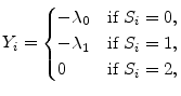
Granularity Adjustment for Mark-to-Market Credit Risk Models*
Keywords: Granularity adjustment, idiosyncratic risk, portfolio credit risk, value-at-risk, expected shortfall
Abstract:
In the portfolio risk-factor frameworks that underpin both industry models of credit value-at-risk (VaR) and the Internal Ratings-Based (IRB) risk weights of Basel II, credit risk in a portfolio arises from two sources, systematic and idiosyncratic. Systematic factors represent the effect of unexpected changes in macroeconomic and financial market conditions on the performance of borrowers. Borrowers may differ in their degree of sensitivity to systematic risk, but few firms are completely insulated from the wider economic conditions in which they operate. Therefore, the systematic component of portfolio risk is unavoidable and only partly diversifiable. Idiosyncratic factors represent the risks that are particular to individual borrowers. As a portfolio becomes more fine-grained, in the sense that the largest individual exposures account for a vanishing share of total portfolio exposure, idiosyncratic risk is diversified away at the portfolio level.
In some settings, including the IRB approach of Basel II, the computation of VaR is dramatically simplified if it is assumed that bank portfolios are perfectly fine-grained, that is, that idiosyncratic risk has been fully diversified away, so that portfolio loss depends only on systematic risk. Real-world portfolios are not, of course, perfectly fine-grained. When there are material name concentrations of exposure, there will be a residual of undiversified idiosyncratic risk in the portfolio. The impact of undiversified idiosyncratic risk on VaR can be approximated analytically via a methodology known as granularity adjustment. In principle, the granularity adjustment (GA) can be applied to any risk-factor model of portfolio credit risk. Thus far, however, analytical results have been derived only for simple models of actuarial loss, i.e., credit loss due to default. The implicit view appears to be that the GA would be tedious to derive, or perhaps even intractable, for the more complicated models of mark-to-market credit loss. Large banks typically model credit loss in market value terms, and even the model underpinning the IRB approach of Basel II is in this advanced class.1 In this paper, we demonstrate that the GA is in fact entirely tractable for a large class of models that includes single-factor versions of all the commonly used mark-to-market approaches. If notation is chosen judiciously, the resulting derivations and calculations are concise and straightforward.
In Section 1, we review the established results in the literature on granularity adjustment and introduce the basic notation. Our general solution for mark-to-market models is given in Section 2. This solution covers both finite ratings-based models and models with a continuum of obligor states. In Section 3, we apply our methodology to CreditMetrics and KMV Portfolio Manager as these are the benchmark models for the finite and continuous classes, respectively. Comparative statics with respect to model parameters are explored in Section 4. Some of the comparative statics appear counterintuitive at first glance, so in Section 5 we explain these results with a stylized model of portfolio risk.
1 Granularity adjustment
For simplicity in exposition, we first consider risk-measurement for a portfolio of ![]() homogeneous positions. We wish to model the portfolio loss rate,
homogeneous positions. We wish to model the portfolio loss rate, ![]() , at a fixed horizon
, at a fixed horizon ![]() with current time normalized to
with current time normalized to ![]() . Let
. Let ![]() denote the loss at the horizon on position
denote the loss at the horizon on position ![]() (expressed as a percentage of current value), so that the portfolio loss rate is simply
(expressed as a percentage of current value), so that the portfolio loss rate is simply
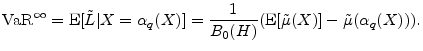
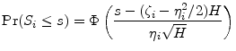
For a given target solvency probability
In terms of this more general notation, VaR is
Let ![]() denote the set of systematic risk factors that are realized at the horizon. A critical assumption of all risk-factor portfolio models is that all dependence in loss across positions
is due to common dependence on
denote the set of systematic risk factors that are realized at the horizon. A critical assumption of all risk-factor portfolio models is that all dependence in loss across positions
is due to common dependence on ![]() , so that
, so that ![]() is independent of
is independent of ![]() when conditioned on
when conditioned on ![]() . As
. As ![]() grows to infinity, all idiosyncratic sources of risk vanish, so
grows to infinity, all idiosyncratic sources of risk vanish, so
![]() , almost surely. This implies that
, almost surely. This implies that
![]() as
as
![]() . This result is especially useful when
. This result is especially useful when ![]() is univariate and
conditional expected loss is increasing in
is univariate and
conditional expected loss is increasing in ![]() , and we henceforth impose these assumptions. Subject to mild restrictions,
, and we henceforth impose these assumptions. Subject to mild restrictions,
![]() is equal to
is equal to
![]() , which is easily calculated in analytical form.
, which is easily calculated in analytical form.
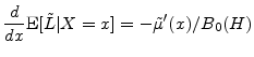
The difference
![]() represents the effect of undiversified idiosyncratic risk in the portfolio. This
difference cannot be obtained in analytical form, but we can construct an asymptotic approximation in orders of
represents the effect of undiversified idiosyncratic risk in the portfolio. This
difference cannot be obtained in analytical form, but we can construct an asymptotic approximation in orders of ![]() .
.
where
The GA extends naturally to heterogeneous portfolios. Let ![]() be the current size of exposure
be the current size of exposure ![]() . This is the face value of the instrument in an actuarial setting, and is the current market value in a mark-to-market setting. Let
. This is the face value of the instrument in an actuarial setting, and is the current market value in a mark-to-market setting. Let
![]() be the portfolio weights. Imposing minor restrictions on the sequence
be the portfolio weights. Imposing minor restrictions on the sequence
![]() so that the
so that the
![]() as
as
![]() (see Assumption (
(see Assumption (
![]() ) in Gordy, 2003), we have
) in Gordy, 2003), we have
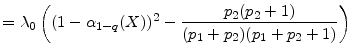
This form of the GA was first suggested by Wilde (2001). Martin and Wilde (2002) gave a more rigorous derivation of Wilde's formula based on theoretical work by Gouriéroux, Laurent, and Scaillet (2000). Gordy (2004) presents a survey of these developments and a primer on the mathematical derivation.2
The GA of equation (4) applies under either accounting paradigm for loss.3 Under an actuarial definition, loss ![]() on position
on position ![]() is the product of a default indicator for
is the product of a default indicator for ![]() and the loss given default (LGD) suffered on that position. LGD is expressed as a percentage of exposure and may itself be stochastic. Heretofore, all applications of the GA to portfolio credit risk have been in an actuarial
setting. Wilde (2001) provides analytical solutions to equation (4) for the CreditRisk
and the loss given default (LGD) suffered on that position. LGD is expressed as a percentage of exposure and may itself be stochastic. Heretofore, all applications of the GA to portfolio credit risk have been in an actuarial
setting. Wilde (2001) provides analytical solutions to equation (4) for the CreditRisk![]() model and for an actuarial version of
the CreditMetrics model. Analysis of CreditMetrics is developed further by Emmer and Tasche (2005). Even for the special case of a homogeneous portfolio and zero recovery on defaulted loans, the Emmer and Tasche solution suggests some complexity. Expressed in the
notation to be introduced below, we have
model and for an actuarial version of
the CreditMetrics model. Analysis of CreditMetrics is developed further by Emmer and Tasche (2005). Even for the special case of a homogeneous portfolio and zero recovery on defaulted loans, the Emmer and Tasche solution suggests some complexity. Expressed in the
notation to be introduced below, we have

The original result, in Emmer and Tasche (2005, Remark 2.3), incorrectly has a minus sign in place of the second plus sign on the second line of equation (5). The same sign error is found in the more general result in Proposition 2.2 of that paper. The obscurity of this error, which we believe has not been noticed until now, perhaps reflects the opacity of the formulae.
In a mark-to-market setting, "loss" is an ambiguous concept. One needs to choose a reference point (i.e., the value of the instrument that counts as zero loss) and a convention for discounting to the present. A typical definition is the difference between expected return and realized return,
discounted back to today at the riskfree rate. Return is defined as the ratio of market value at the horizon (inclusive of cashflows received during the period ![]() , accrued to the horizon
at the riskfree rate) to the current market value. We adopt this convention, but note that it is generally trivial to modify our results to accommodate other definitions.
, accrued to the horizon
at the riskfree rate) to the current market value. We adopt this convention, but note that it is generally trivial to modify our results to accommodate other definitions.
To formalize, let ![]() be the money market fund, i.e.,
be the money market fund, i.e., ![]() is the value at
is the value at
![]() of a unit of currency invested at date
of a unit of currency invested at date ![]() in a riskless continuously compounded
money market fund. We can write this as
in a riskless continuously compounded
money market fund. We can write this as
Let
![]() denote the conditional expected return
denote the conditional expected return
![]() as a function of
as a function of ![]() ,
and similarly define
,
and similarly define

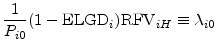
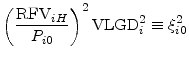
This is the form in which we will calculate the GA.
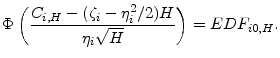
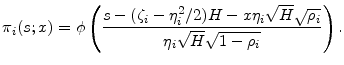
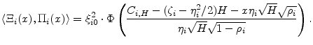
In many commonly-used models, the distribution of ![]() is such that
is such that
![]() takes a simple form. This is most notably the case when
takes a simple form. This is most notably the case when ![]() is normally
distributed (as in the models considered in Section 3), for which we have
is normally
distributed (as in the models considered in Section 3), for which we have
![]() . Here it can be convenient to apply the product rule to the derivative in the GA formula, and arrive at
. Here it can be convenient to apply the product rule to the derivative in the GA formula, and arrive at
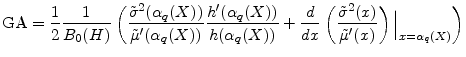
We have thus far assumed that value-at-risk is the risk-measure of interest. A popular alternative to VaR is expected shortfall (ES). When portfolio loss has continuous distribution, this is defined as
Martin and Tasche (2007) and Gordy (2004) show that the granularity adjustment for ES is
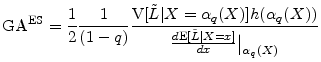
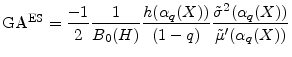
The computations needed for this expression are a subset of the computations needed for equation (7), so it is clear that the ES GA can readily be calculated whenever the VaR GA can be calculated.
Finally, in some models conditional expected loss is monotonically decreasing in ![]() . The above results continue to hold, but with
. The above results continue to hold, but with
![]() everywhere replaced by
everywhere replaced by
![]() and the sign on
and the sign on
![]() reversed.
reversed.
2 Conditional expected return and variance functions
To implement the GA, we require tractable expressions for the conditional expected return and conditional variance of return as functions of the realization of ![]() . We consider first the
class of credit risk models in which the condition of obligors at the horizon is represented by a finite state space. This includes the important class of ratings-based models, for which the "state" is the obligor's rating at the horizon.
. We consider first the
class of credit risk models in which the condition of obligors at the horizon is represented by a finite state space. This includes the important class of ratings-based models, for which the "state" is the obligor's rating at the horizon.
Let
![]() be the set of possible obligor states at the horizon. These states are enumerated as
be the set of possible obligor states at the horizon. These states are enumerated as
![]() . Let
. Let
![]() be the state for obligor
be the state for obligor ![]() at the
horizon. When the states are S&P rating grades, for example, the obligor has defaulted if
at the
horizon. When the states are S&P rating grades, for example, the obligor has defaulted if
![]() , migrated to CCC if
, migrated to CCC if
![]() , and so on up to
, and so on up to
![]() for migration to AAA.
for migration to AAA.
In all ratings-based models, the return
![]() depends on the horizon rating
depends on the horizon rating
![]() . More generally, we might expect
. More generally, we might expect
![]() to be influenced by the systematic factor
to be influenced by the systematic factor ![]() , as prevailing
spreads for a given rating grade typically increase during a credit market downturn. There may also be idiosyncratic influences on the value at the horizon. Many current models allow for idiosyncratic recovery risk (i.e., random LGD) in the default state, and the models could (in principle) easily
be extended to allow for idiosyncratic spread risk in non-default states. In our framework, we allow for all three sources of risk.
, as prevailing
spreads for a given rating grade typically increase during a credit market downturn. There may also be idiosyncratic influences on the value at the horizon. Many current models allow for idiosyncratic recovery risk (i.e., random LGD) in the default state, and the models could (in principle) easily
be extended to allow for idiosyncratic spread risk in non-default states. In our framework, we allow for all three sources of risk.
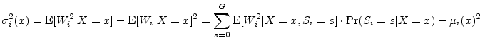
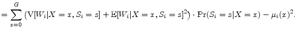
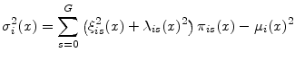
We decompose the conditional expected value by further conditioning on horizon state:
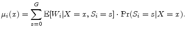
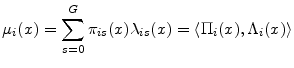
where
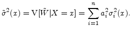
We proceed similarly for the conditional variance:
|
|
 |
Letting
where
We now turn to the class of credit risk models in which the obligor state at the horizon can take on a continuum of values. This includes structural approaches based on the Merton (1974) model in which obligor credit risk can be measured by the standardized distance between the obligor's asset value and default threshold. In industry practice, KMV Portfolio Manager is the most widely-used implementation of this approach.
As before,
![]() is the set of possible obligor states at the horizon. Typically we would have
is the set of possible obligor states at the horizon. Typically we would have
![]() , but that is not strictly necessary for our purposes. Adapting our earlier notation, let
, but that is not strictly necessary for our purposes. Adapting our earlier notation, let
![]() be the conditional probability density function for
be the conditional probability density function for
![]() , and let
, and let
When working with this class of models, let
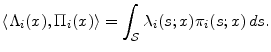
In both the discrete and continuous state space cases, the derivative of the inner product is given by the usual product rule, e.g.,
3 Application
To apply the results of the previous section to a given model, we need to have tractable and differentiable expressions for the
![]() ,
,
![]() and
and
![]() functions. For the models most widely-used in practice, these functions are indeed easily obtained and even more easily differentiated. We demonstrate with application
to CreditMetrics and KMV Portfolio Manager, as these are the benchmark models for the finite and continuous classes, respectively.
functions. For the models most widely-used in practice, these functions are indeed easily obtained and even more easily differentiated. We demonstrate with application
to CreditMetrics and KMV Portfolio Manager, as these are the benchmark models for the finite and continuous classes, respectively.
3.1 CreditMetrics
CreditMetrics is perhaps the most widely-known industry model of portfolio credit risk.4 The model is loosely styled on the classic structural model of
Merton (1974), but is calibrated to credit ratings rather than equity price and balance sheet information. Obligor rating is taken as a sufficient statistic of the term-structure of firm default risk on a single-name basis, and rating transitions are assumed to follow a
time-homogeneous Markov chain. This implies that the unconditional distribution over horizon rating depends only on current rating. We write
![]() for the probability of transition from current grade
for the probability of transition from current grade ![]() to
grade
to
grade ![]() at the horizon.
at the horizon.
Associated with obligor ![]() is a latent "asset return" variable
is a latent "asset return" variable
![]() , which is assumed to be distributed
, which is assumed to be distributed
![]() . The real line is partitioned into "bins" corresponding to the possible state outcomes in
. The real line is partitioned into "bins" corresponding to the possible state outcomes in
![]() . Given current rating
. Given current rating ![]() , the obligor defaults if
, the obligor defaults if
![]() , transitions to CCC if
, transitions to CCC if
![]() , and so on, for fixed bin threshold values
, and so on, for fixed bin threshold values
To induce dependence across obligors, we decompose the asset returns as
The systematic factor
Exploiting the relationship
Relative to the general framework of Section 2, CreditMetrics imposes simplifying assumptions on the distribution of return in each state. Market credit spreads at the horizon are taken as deterministic functions of rating grade. In the case of default, there is only idiosyncratic risk in recovery. Therefore, for all horizon states,
The return in the default state is affine in the recovery rate
![]() . For example, say we have a loan with biannual coupons of
. For example, say we have a loan with biannual coupons of ![]() ,
face value of 1, and current value
,
face value of 1, and current value ![]() . If we assume that default occurs just before the horizon of
. If we assume that default occurs just before the horizon of ![]() year, then the first coupon is received and the second is accrued into the claim. The return in the default state is therefore
year, then the first coupon is received and the second is accrued into the claim. The return in the default state is therefore
![]() . In the CreditMetrics model, it is assumed that
. In the CreditMetrics model, it is assumed that
![]() is drawn as an independent beta-distributed random variable with specified mean
is drawn as an independent beta-distributed random variable with specified mean
![]() and variance
and variance
![]() , which implies that
, which implies that
![]() is affine in
is affine in
![]() and
and
![]() is affine in
is affine in
![]() . For parsimony in data requirements, it is usually assumed that
. For parsimony in data requirements, it is usually assumed that
for fixed volatility parameter
At this point in the analysis, only the state returns
![]() remain to be calculated. In the original version of CreditMetrics, as documented by Gupton et al. (1997), pricing at the horizon followed
a discounted contractual cashflow approach. For greater internal consistency, later versions of CreditMetrics adopted a modified version of the Hull and White (2000) methodology. In this approach, the term-structures of risk-neutral default probabilities for each grade
are backed out from the observed term-structures of ratings-based credit spreads. It is then trivial to obtain prices for each obligor rating at the horizon by summing the discounted expected cashflows. For our purposes in this paper, either methodology (or, indeed, any number of other pricing
methodologies) can be used. One must be able to calculate the return in each obligor state in order to implement CreditMetrics, so the calculation of the
remain to be calculated. In the original version of CreditMetrics, as documented by Gupton et al. (1997), pricing at the horizon followed
a discounted contractual cashflow approach. For greater internal consistency, later versions of CreditMetrics adopted a modified version of the Hull and White (2000) methodology. In this approach, the term-structures of risk-neutral default probabilities for each grade
are backed out from the observed term-structures of ratings-based credit spreads. It is then trivial to obtain prices for each obligor rating at the horizon by summing the discounted expected cashflows. For our purposes in this paper, either methodology (or, indeed, any number of other pricing
methodologies) can be used. One must be able to calculate the return in each obligor state in order to implement CreditMetrics, so the calculation of the
![]() imposes no burden that is peculiar to granularity adjustment.
imposes no burden that is peculiar to granularity adjustment.
Finally, we note that the GA for the actuarial version of CreditMetrics can be obtained as a special case with our general framework. To calculate the actuarial GA, fix
![]() for all non-default
for all non-default ![]() ,
,
![]() and
and
![]() , and fix both the coupon rate and the riskfree rate to zero. The GA formula of Emmer and Tasche (2005)
is a special case of our formula in which ELGD is fixed to 1 and VLGD to zero.
, and fix both the coupon rate and the riskfree rate to zero. The GA formula of Emmer and Tasche (2005)
is a special case of our formula in which ELGD is fixed to 1 and VLGD to zero.
3.2 KMV Portfolio Manager
Like CreditMetrics, Moody's KMV model is based on the classic structural model of Merton (1974). Whereas CreditMetrics takes a stylized approach to the model, KMV is firmly grounded in the substance of the structural relationship between firm asset value and debt performance. The model can be divided into two components. Default prediction (i.e., estimation of the term-structure of firm default probabilities, or "EDFs") is provided by KMV Credit Monitor (Crosbie and Bohn, 2003; Kealhofer, 2003a). Portfolio risk is assessed by KMV Portfolio Manager (Kealhofer and Bohn, 2001). We develop the GA for version 1.4 of KMV Portfolio Manager, and note that the current version of the model may differ in important respects.
The portfolio model takes as input the term-structure of EDFs for each obligor in the portfolio, and we do the same here. Specifically, for each firm ![]() , we take as input parameters the
probability of default at or before the horizon (
, we take as input parameters the
probability of default at or before the horizon (
![]() ) and the probability of default at or before loan maturity (
) and the probability of default at or before loan maturity (
![]() ).
).
In the structural approach, default occurs when asset value falls short of the fixed liabilities of the firm at ![]() . We take as the obligor state variable the log return on firm assets. The
asset value is assumed to follow a geometric Brownian motion with drift under the physical measure, so that
. We take as the obligor state variable the log return on firm assets. The
asset value is assumed to follow a geometric Brownian motion with drift under the physical measure, so that
where
where the systematic factor
The domain of possible states at the horizon is the real line. Because the shocks are normally distributed, it is easily seen that the cdf of
![]() is
is
The default threshold
The conditional distribution of
![]() is also Gaussian. It is easily seen that the conditional density is
is also Gaussian. It is easily seen that the conditional density is
The KMV pricing algorithm differs from that of CreditMetrics, but shares the important assumptions that market value at the horizon is a deterministic function of obligor state for surviving obligors, and that, in the case of default, there is only idiosyncratic risk in recovery. Therefore, for all horizon states,
The KMV pricing methodology separates future contractual cashflows into riskless and risky components. If recovery were deterministic, we would write for the price ![]() of a loan at time
of a loan at time
![]()
where
In the event of default at or before the horizon, the value at the horizon is
![]() . While this recovery value is stochastic, it is invariant with respect to
. While this recovery value is stochastic, it is invariant with respect to
![]() , so we can write
, so we can write
 |
|||
 |
for all
In the event of survival, the return is
![]() . We write
. We write ![]() as a function of horizon state because of
the dependence of
as a function of horizon state because of
the dependence of
![]() on
on
![]() . The calculation of
. The calculation of
![]() is detailed in Gordy, Heitfield, and Jones (in progress). As we have noted in the context of the CreditMetrics model, one must be
able to calculate the return in each obligor state in order to implement the portfolio model, so the calculation of the
is detailed in Gordy, Heitfield, and Jones (in progress). As we have noted in the context of the CreditMetrics model, one must be
able to calculate the return in each obligor state in order to implement the portfolio model, so the calculation of the
![]() imposes no burden that is peculiar to granularity adjustment.
imposes no burden that is peculiar to granularity adjustment.
4 Comparative Statics
In this section, we explore the comparative statics of the granularity adjustment with special emphasis on the parameters that do not appear under the actuarial paradigm. For the sake of clarity, we adopt the CreditMetrics model in a stylized setting with two non-default rating grades
(![]() ). We consider a portfolio that is homogeneous in all respects other than initial credit rating, i.e., all loans are of equal size and have the same
). We consider a portfolio that is homogeneous in all respects other than initial credit rating, i.e., all loans are of equal size and have the same
![]() and
and
![]() , and all obligors have the same asset correlation
, and all obligors have the same asset correlation ![]() .
If all obligors were of the same initial rating as well, then we know from equation (3) that the GA can be written as
.
If all obligors were of the same initial rating as well, then we know from equation (3) that the GA can be written as ![]() for
for ![]() that depends on model parameters but not on
that depends on model parameters but not on ![]() . When obligors are not of the same initial
rating, the GA can still be written as
. When obligors are not of the same initial
rating, the GA can still be written as ![]() if we fix the share of each rating grade in the portfolio. We present the comparative statics in terms of
if we fix the share of each rating grade in the portfolio. We present the comparative statics in terms of ![]() to avoid dependence on the choice of
to avoid dependence on the choice of ![]() .
.
We parameterize the matrix of unconditional transition probabilities (under the physical measure) as in Table 1. Default probabilities are
![]() and
and
![]() . In our baseline parameterization, we set
. In our baseline parameterization, we set
![]() to 15 basis points (bp) and
to 15 basis points (bp) and
![]() to 300bp, so that grades A and B represent the investment and speculative grades, respectively. Conditional on survival, the probability of remaining in the initial grade
is
to 300bp, so that grades A and B represent the investment and speculative grades, respectively. Conditional on survival, the probability of remaining in the initial grade
is
![]() . Agency ratings are known to be "sticky" (Löffler, 2004;
Altman and Rijken, 2004), so we set
. Agency ratings are known to be "sticky" (Löffler, 2004;
Altman and Rijken, 2004), so we set
![]() .
.
Our baseline portfolio is composed of equal numbers of grade A and grade B loans. Each loan has face value 1, ELGD of 50%, and maturity of 3 years. Coupons are paid biannually. In the event of default, it is assumed that the first coupon is received in full, and the second coupon is accrued into
the legal claim in bankruptcy. Asset correlation is fixed at ![]() . The riskfree rate is a constant
. The riskfree rate is a constant ![]() and the variance parameter for LGD is
and the variance parameter for LGD is
![]() . The horizon is
. The horizon is ![]() year and the target solvency
probability is
year and the target solvency
probability is ![]() .
.
For consistency with the current generation of CreditMetrics, we use the pricing approach of Hull and White (2000). This requires that we have for each obligor the term-structure of risk-neutral cumulative default probabilities, which in practical application is
extracted from the observed term-structure of credit spreads. For our purposes, a parametric approach is preferable, so we obtain the risk-neutral term structure of default probabilities by adding a parameterized risk-premium to the term structure of default probabilities under the physical
measure. Since the CreditMetrics model assumes that ratings follow a time-homogeneous Markov process, we can take powers of the transition matrix in Table 1 to obtain the physical cumulative default probability at any horizon. Let
![]() denote the physical probability of default between time
denote the physical probability of default between time ![]() and time
and time ![]() for an obligor in grade
for an obligor in grade ![]() at time
at time ![]() . The Markovian structure of the model implies that
. The Markovian structure of the model implies that
![]() . We convert to risk-neutral probabilities
. We convert to risk-neutral probabilities
![]() as in the KMV model:
as in the KMV model:
Our comparative statics are total derivatives. As parameter values change, the par coupon for the loans will change as well. To take the total derivative of ![]() with respect to,
say,
with respect to,
say,
![]() , we maintain the initial par value of each loan by changing the coupon to its par value for each value of
, we maintain the initial par value of each loan by changing the coupon to its par value for each value of
![]() . This approach is most consistent with economic intuition.
. This approach is most consistent with economic intuition.
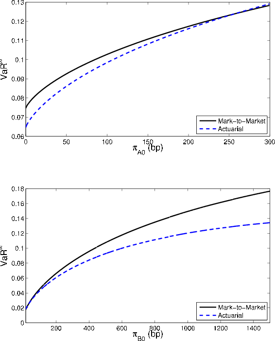
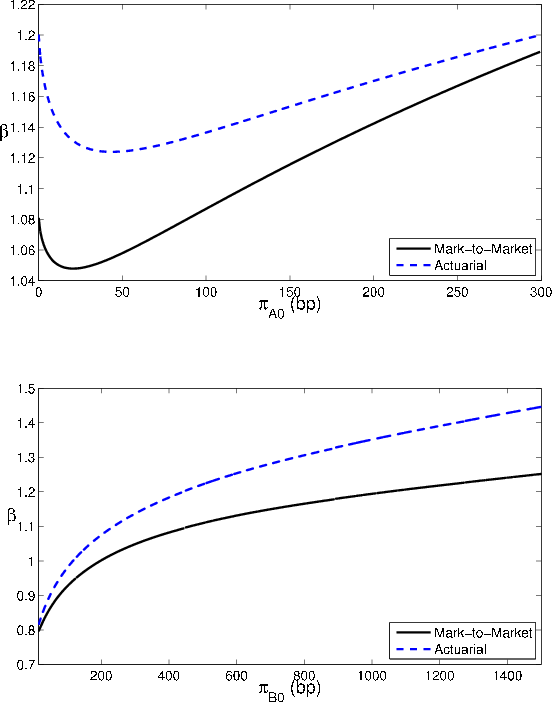
We first explore sensitivity of asymptotic VaR and the GA to parameters that appear in both the MtM and actuarial models, starting with default probabilities
![]() . In the upper panel of Figure 1, we vary
. In the upper panel of Figure 1, we vary
![]() from zero to 300bp while holding
from zero to 300bp while holding
![]() fixed to its baseline value of 300bp. In the lower panel, we vary
fixed to its baseline value of 300bp. In the lower panel, we vary
![]() from 15bp to 1500bp while holding
from 15bp to 1500bp while holding
![]() fixed to its baseline value of 15bp. As we should expect, asymptotic VaR, denoted
fixed to its baseline value of 15bp. As we should expect, asymptotic VaR, denoted
![]() and defined as
and defined as
![]() , is increasing monotonically with both default probabilities under both actuarial and MtM paradigms.5 VaR is larger in the MtM setting because it captures migration risk and loss of coupon income in the event of default. When
, is increasing monotonically with both default probabilities under both actuarial and MtM paradigms.5 VaR is larger in the MtM setting because it captures migration risk and loss of coupon income in the event of default. When
![]() , migration risk is eliminated, so the two views of risk are nearly equivalent.
, migration risk is eliminated, so the two views of risk are nearly equivalent.
Comparative statics for the GA are displayed in Figure 1. Except at low values of
![]() , the GA increases in the default probabilities. The intuition, which we will develop in greater detail in Section 5, is that extreme losses in
the finite portfolio case are most likely to be generated by a combination of unfavorable systematic and idiosyncratic draws, rather than by systematic risk alone. Default events induce larger loss than downgrades, so the idiosyncratic effect will manifest as a higher than conditionally expected
default rate. This implies that VaR is more sensitive to default risk than asymptotic
, the GA increases in the default probabilities. The intuition, which we will develop in greater detail in Section 5, is that extreme losses in
the finite portfolio case are most likely to be generated by a combination of unfavorable systematic and idiosyncratic draws, rather than by systematic risk alone. Default events induce larger loss than downgrades, so the idiosyncratic effect will manifest as a higher than conditionally expected
default rate. This implies that VaR is more sensitive to default risk than asymptotic
![]() , and therefore that the gap between them should increase with
, and therefore that the gap between them should increase with
![]() .
.
This intuition breaks down when the grade A default probability is very low. For small
![]() , it takes a large (and therefore unlikely) idiosyncratic shock to cause a grade A firm to default even when
, it takes a large (and therefore unlikely) idiosyncratic shock to cause a grade A firm to default even when
![]() . Consequently, for any given realization of the set of idiosyncratic shocks (i.e., the
. Consequently, for any given realization of the set of idiosyncratic shocks (i.e., the
![]() of equation (12)), portfolio loss is largest for permutations that disproportionately assign negative shocks to grade B firms. As the
scenarios associated with VaR in the finite portfolio case will be disproportionately driven by grade B defaults, VaR must be less sensitive to
of equation (12)), portfolio loss is largest for permutations that disproportionately assign negative shocks to grade B firms. As the
scenarios associated with VaR in the finite portfolio case will be disproportionately driven by grade B defaults, VaR must be less sensitive to
![]() than asymptotic
than asymptotic
![]() . For this counterintuitive effect to be observed, we must have positive portfolio shares in at least two non-default grades. If we have only a single
non-default grade, then
. For this counterintuitive effect to be observed, we must have positive portfolio shares in at least two non-default grades. If we have only a single
non-default grade, then ![]() is strictly increasing with the unconditional default probability.
is strictly increasing with the unconditional default probability.
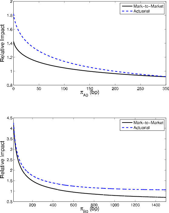
The relative impact of the GA is plotted in Figure 1. For a portfolio of ![]() , define the relative impact as the ratio of the GA to VaR, where the portfolio
VaR is approximated as the sum of asymptotic
, define the relative impact as the ratio of the GA to VaR, where the portfolio
VaR is approximated as the sum of asymptotic
![]() and the GA, i.e.,
and the GA, i.e.,
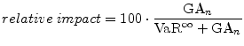
The lower the default probabilities, the greater the relative importance of sampling variation on portfolio risk, so the larger is the GA as a share of VaR.
The effect of portfolio quality on asymptotic
![]() and the GA is consistent with the comparative statics for default probabilities. We find that
and the GA is consistent with the comparative statics for default probabilities. We find that
![]() and the GA both fall with the share of grade A in the portfolio. The MtM
and the GA both fall with the share of grade A in the portfolio. The MtM
![]() exceeds the actuarial
exceeds the actuarial
![]() at all values of the investment-grade share, but the actuarial GA exceeds the MtM GA. On a relative impact basis, we find that the size of the GA is increasing
with the share of grade A.
at all values of the investment-grade share, but the actuarial GA exceeds the MtM GA. On a relative impact basis, we find that the size of the GA is increasing
with the share of grade A.
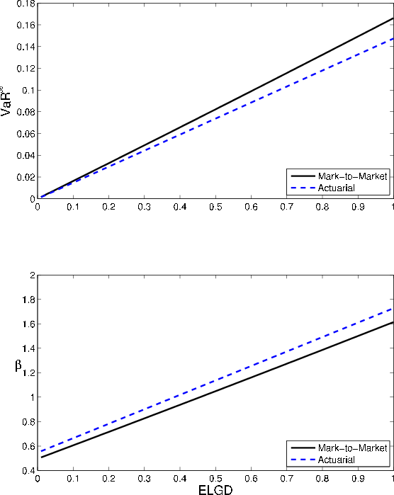
Comparative statics for recovery rates, shown in Figure 2, are also similar to those for default probabilities. Both asymptotic
![]() and the GA increase with ELGD. The relationships are exactly linear in the actuarial setting, and nearly non-linear in the MtM case (i.e., there is a slight
non-linearity due to the effect of ELGD on par spread). The GA increases with ELGD because ELGD controls the magnitude of loss in the default state and, as we have just observed, the finite-portfolio VaR is more sensitive than the asymptotic
and the GA increase with ELGD. The relationships are exactly linear in the actuarial setting, and nearly non-linear in the MtM case (i.e., there is a slight
non-linearity due to the effect of ELGD on par spread). The GA increases with ELGD because ELGD controls the magnitude of loss in the default state and, as we have just observed, the finite-portfolio VaR is more sensitive than the asymptotic
![]() to default risk.
to default risk.
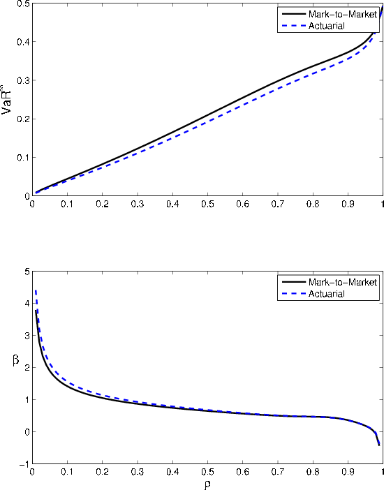
Comparative statics for asset correlation are relatively straightforward. As shown in the upper panel of Figure 3, asymptotic VaR is strictly increasing in ![]() . At
. At ![]() , all risk is diversifiable, so
, all risk is diversifiable, so
![]() is zero. At
is zero. At ![]() , asset returns are comonotonic.
So long as
, asset returns are comonotonic.
So long as
![]() , all borrowers default in the state
, all borrowers default in the state
![]() , and
, and
![]() is determined primarily by
is determined primarily by
![]() . Between these two extremes,
. Between these two extremes,
![]() increases monotonically.
increases monotonically.
The effect of asset correlation on the GA runs in the opposite direction, as seen in the bottom panel of Figure 3. The greater is ![]() , the smaller the
impact of idiosyncratic risk on asset returns, so the smaller the contribution of idiosyncratic risk to VaR. As
, the smaller the
impact of idiosyncratic risk on asset returns, so the smaller the contribution of idiosyncratic risk to VaR. As ![]() falls to zero, one can show analytically that
falls to zero, one can show analytically that ![]() tends to infinity. As
tends to infinity. As ![]() increases to one,
increases to one, ![]() can tend to negative infinity (when
can tend to negative infinity (when
![]() and
and
![]() ) or to zero (when
) or to zero (when
![]() or when
or when
![]() ), or even to positive infinity (in a subset of the remaining cases). At these endpoints, the asymptotic series underpinning equation (3) diverges, so the first-order GA becomes an unreliable measure of the gap between VaR and asymptotic
), or even to positive infinity (in a subset of the remaining cases). At these endpoints, the asymptotic series underpinning equation (3) diverges, so the first-order GA becomes an unreliable measure of the gap between VaR and asymptotic
![]() .6 Nonetheless,
negative values for
.6 Nonetheless,
negative values for ![]() are not just an artifact. When
are not just an artifact. When ![]() is near one, the
density of the loss distribution becomes multimodal, and in this circumstance asymptotic
is near one, the
density of the loss distribution becomes multimodal, and in this circumstance asymptotic
![]() can exceed VaR. Martin and Tasche (2007) explain this phenomenon as a concomitant of the failure of sub-additivity in VaR and prove
that the granularity adjustment for expected shortfall is always positive.
can exceed VaR. Martin and Tasche (2007) explain this phenomenon as a concomitant of the failure of sub-additivity in VaR and prove
that the granularity adjustment for expected shortfall is always positive.
We can assess the impact of recovery risk through the comparative static with respect to
![]() . Asymptotic VaR is invariant with respect to idiosyncratic recovery risk, so is invariant with respect to
. Asymptotic VaR is invariant with respect to idiosyncratic recovery risk, so is invariant with respect to
![]() . The GA is linear and increasing in
. The GA is linear and increasing in
![]() , so also is linear and increasing in
, so also is linear and increasing in
![]() . The effect is generally large. In our baseline example, the slope
. The effect is generally large. In our baseline example, the slope
![]() is 1.004 for the MtM model and 1.092 for the actuarial model.
is 1.004 for the MtM model and 1.092 for the actuarial model.
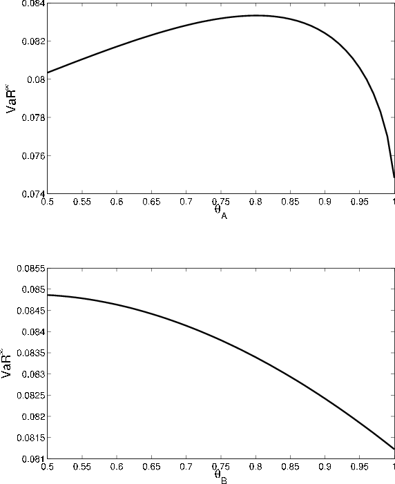
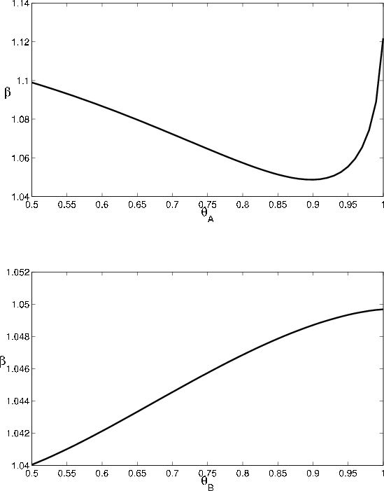
We now turn to the parameters that influence risk under the mark-to-market paradigm, but not the actuarial model. The parameter ![]() controls the degree of stickiness in ratings,
conditional on survival to the horizon. In an actuarial setting, asymptotic
controls the degree of stickiness in ratings,
conditional on survival to the horizon. In an actuarial setting, asymptotic
![]() and the GA are invariant with respect to non-default transition likelihood. The comparative statics in the MtM setting are somewhat complicated and perhaps
surprising. Consider first the effect of varying
and the GA are invariant with respect to non-default transition likelihood. The comparative statics in the MtM setting are somewhat complicated and perhaps
surprising. Consider first the effect of varying ![]() on asymptotic
on asymptotic
![]() . As
. As ![]() increases, the conditional and
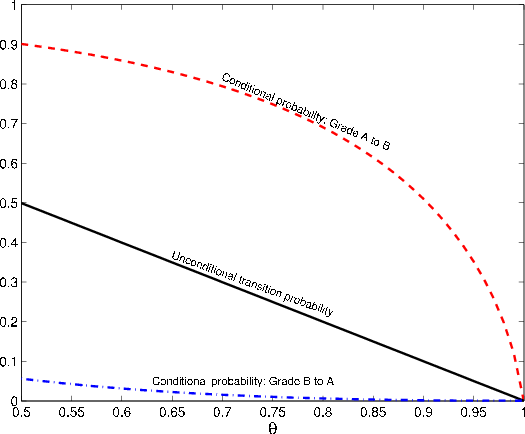
unconditional probabilities of transition from B to A both fall towards zero. Because the conditional probability is already low (i.e., one expects few upgrades when conditioning on a bad systematic draw), the unconditional probability falls by more than the conditional probability, as seen in
Figure 4. This closes the gap between
increases, the conditional and
unconditional probabilities of transition from B to A both fall towards zero. Because the conditional probability is already low (i.e., one expects few upgrades when conditioning on a bad systematic draw), the unconditional probability falls by more than the conditional probability, as seen in
Figure 4. This closes the gap between
![]() and
and
![]() , so reduces
, so reduces
![]() (lower panel of Figure 5).
(lower panel of Figure 5).
For ![]() , the story is somewhat more complicated. As seen in Figure 4, the gap between the conditional and unconditional probability of transition from A
to B is fairly constant over
, the story is somewhat more complicated. As seen in Figure 4, the gap between the conditional and unconditional probability of transition from A
to B is fairly constant over
![]() and then converges rapidly to zero as
and then converges rapidly to zero as ![]() increases
towards one. In the lower range, the effect on
increases
towards one. In the lower range, the effect on
![]() is dominated by the indirect effect on par coupon rates: as
is dominated by the indirect effect on par coupon rates: as ![]() increases, the par coupon for grade A falls, so the return
increases, the par coupon for grade A falls, so the return
![]() associated with downgrade to B is reduced.7 The probability weight on
associated with downgrade to B is reduced.7 The probability weight on
![]() is greater under the conditional distribution than the unconditional, so the gap between
is greater under the conditional distribution than the unconditional, so the gap between
![]() and
and
![]() widens. However, in the upper range of
widens. However, in the upper range of ![]() values, the rapid convergence of
values, the rapid convergence of
![]() towards
towards
![]() dominates, and this causes
dominates, and this causes
![]() to decrease with
to decrease with ![]() . This non-monotonic
behavior is observed in the upper panel of Figure 5.
. This non-monotonic
behavior is observed in the upper panel of Figure 5.
The comparative statics for the GA as a function of ![]() , displayed in Figure 5, are the mirror image of the comparative statics for VaR. The intuition
is similar to the explanation for the comparative statics with respect to the
, displayed in Figure 5, are the mirror image of the comparative statics for VaR. The intuition
is similar to the explanation for the comparative statics with respect to the
![]() . Relative to asymptotic
. Relative to asymptotic
![]() , finite portfolio VaR is more sensitive to default risk and less sensitive to migration risk. This implies that the GA will increase (decrease) with
, finite portfolio VaR is more sensitive to default risk and less sensitive to migration risk. This implies that the GA will increase (decrease) with
![]() whenever
whenever
![]() decreases (increases) with
decreases (increases) with ![]() .
.
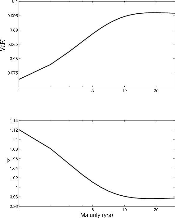
Loan maturity increases the sensitivity of returns to rating migration, so asymptotic
![]() increases with maturity. At long maturities, the return distribution reflects the long-run steady-state of the rating process, so the relationship becomes flat.
This is seen in Figure 6, where we plot VaR against maturity (log-scale) in the upper panel. Similar to the phenomenom observed in the comparative statics for
increases with maturity. At long maturities, the return distribution reflects the long-run steady-state of the rating process, so the relationship becomes flat.
This is seen in Figure 6, where we plot VaR against maturity (log-scale) in the upper panel. Similar to the phenomenom observed in the comparative statics for ![]() , and indeed for the very same reason, the comparative statics for GA (lower panel) with respect to maturity are the mirror image of the comparative statics for asymptotic
, and indeed for the very same reason, the comparative statics for GA (lower panel) with respect to maturity are the mirror image of the comparative statics for asymptotic
![]() .
.
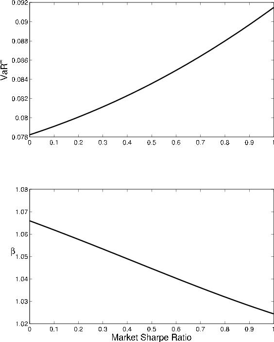
Comparative statics with respect to the market Sharpe ratio parameter follow the same logic. The higher the risk premium
![]() , the larger the loss associated with downward migration, so the higher the asymptotic
, the larger the loss associated with downward migration, so the higher the asymptotic
![]() (upper panel of Figure 7). Parallel to the pattern observed for
(upper panel of Figure 7). Parallel to the pattern observed for ![]() and maturity, the comparative statics for the GA with respect to
and maturity, the comparative statics for the GA with respect to
![]() are the mirror image of the comparative statics for
are the mirror image of the comparative statics for
![]() (lower panel).
(lower panel).
Finally, comparative statics for the riskfree rate are quite straightforward. Both VaR and the GA decline in near linear fashion with the money market return ![]() , because the riskfree
rate has a minimal effect on valuation at the horizon.
, because the riskfree
rate has a minimal effect on valuation at the horizon.
5 A beta-trinomial model of portfolio risk
For parameters governing migration risk in CreditMetrics, we have observed a curious "mirror image" pattern, whereby the comparative static for the GA is of opposite sign to the comparative static for asymptotic
![]() . For parameters governing default risk, by contrast, both
. For parameters governing default risk, by contrast, both
![]() and the GA are increasing (except in one corner of the parameter space). In this section, we shed light on these phenomena using a stylized model of portfolio
risk. The comparative statics of this simple model lack the complexity and nuance of the patterns in CreditMetrics, but the most salient characteristics are preserved.
and the GA are increasing (except in one corner of the parameter space). In this section, we shed light on these phenomena using a stylized model of portfolio
risk. The comparative statics of this simple model lack the complexity and nuance of the patterns in CreditMetrics, but the most salient characteristics are preserved.
We assume a homogeneous portfolio of ![]() positions and specify the return on position
positions and specify the return on position ![]() as
as
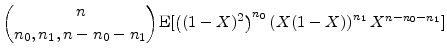
Let the risk factor ![]() be distributed Beta
be distributed Beta
![]() on the unit interval. Conditional on
on the unit interval. Conditional on ![]() , the
state probabilities for
, the
state probabilities for
![]() are
are
![]() . The
. The
![]() are assumed to be mutually independent and independent of
are assumed to be mutually independent and independent of ![]() and
all other risks. Conditional on
and
all other risks. Conditional on
![]() ,
,
![]() is the only source of uncertainty, so
is the only source of uncertainty, so
![]() .
.
If we assume for parsimony that investors are risk-neutral, then in equilibrium the constant ![]() is chosen so that
is chosen so that
![]() . This is solved analytically as
. This is solved analytically as
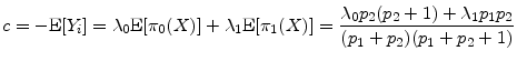
where the last equality follows from the moments of the beta distribution. When we impose this choice of
Besides the portfolio size ![]() , the model has only five parameters:
, the model has only five parameters:
![]() . The parameter of greatest interest is
. The parameter of greatest interest is
![]() , because it determines the magnitude of loss in the downgrade state (
, because it determines the magnitude of loss in the downgrade state (
![]() ). Parameter
). Parameter
![]() determines the magnitude of loss in the default state (
determines the magnitude of loss in the default state (
![]() ), and corresponds most directly to ELGD in CreditMetrics. We restrict
), and corresponds most directly to ELGD in CreditMetrics. We restrict
![]() , so that default induces larger loss than downgrade. Parameters
, so that default induces larger loss than downgrade. Parameters
![]() jointly control the distribution of systematic risk. The higher is
jointly control the distribution of systematic risk. The higher is
![]() relative to
relative to
![]() , the higher the probability of the "good state,"
, the higher the probability of the "good state,"
![]() . Increasing both parameters in proportion leaves the expected value of
. Increasing both parameters in proportion leaves the expected value of ![]() unchanged but shrinks its variance. In our examples below, we fix
unchanged but shrinks its variance. In our examples below, we fix
![]() and take
and take
![]() as our baseline value. The final parameter has the narrow purpose of smoothing the return distribution. We aim to choose the smallest value that will be sufficient to
eliminate humps in the density function. In our examples below, we fix
as our baseline value. The final parameter has the narrow purpose of smoothing the return distribution. We aim to choose the smallest value that will be sufficient to
eliminate humps in the density function. In our examples below, we fix
![]() .
.
The model yields analytical solutions for the GA and for the moments, density and cdf of the return distribution. It is already clear that we have simple expressions for the conditional mean
![]() and variance
and variance
![]() and for the derivatives of these functions. For the beta density for
and for the derivatives of these functions. For the beta density for ![]() , we have
, we have
 |
|||
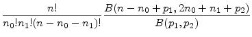 |
where
 |
(22) |
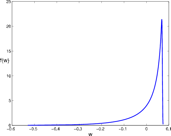
The density of
In Figure 8, we plot the density of the return distribution under our baseline parameter assumptions. The coefficients of skewness and kurtosis are -2.3 and 10.1, respectively, which is qualitatively suitable for the distribution of log-return in a credit
portfolio.8 If we decrease
![]() or increase
or increase
![]() , the distribution would flatten out and become less asymmetric.
, the distribution would flatten out and become less asymmetric.
Asymptotic VaR for this model is easily obtained:
 |
|
 |
(23) |
where in the last equality we substitute the equilibrium value for
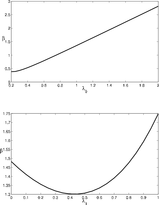
Comparative statics for the GA are depicted in Figure 9.9 As shown in the upper panel, ![]() is increasing with
is increasing with
![]() . The relationship for
. The relationship for
![]() , shown in the lower panel, is non-monotonic. The slope
, shown in the lower panel, is non-monotonic. The slope ![]() is decreasing with
is decreasing with
![]() at low values of
at low values of
![]() and increasing at higher values of
and increasing at higher values of
![]() . In practical application,
. In practical application,
![]() takes on low values (less than the baseline value of 0.2) because loss due to downgrade is generally much smaller than loss due to default.10 Thus, as observed for CreditMetrics, the GA in this model can increase with default loss and decrease with migration loss while asymptotic
takes on low values (less than the baseline value of 0.2) because loss due to downgrade is generally much smaller than loss due to default.10 Thus, as observed for CreditMetrics, the GA in this model can increase with default loss and decrease with migration loss while asymptotic
![]() is increasing in both parameters.
is increasing in both parameters.
The GA is decreasing in
![]() because migration risk has a smaller impact on VaR for the finite portfolio than it does for the asymptotic portfolio. To see this, consider first the probability of
downgrade,
because migration risk has a smaller impact on VaR for the finite portfolio than it does for the asymptotic portfolio. To see this, consider first the probability of
downgrade,
![]() , conditional on a given level of portfolio loss, i.e.,
, conditional on a given level of portfolio loss, i.e.,
![]() . For the finite portfolio case,
. For the finite portfolio case,
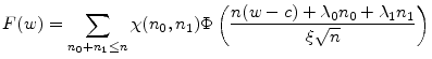
where the last equality is easily derived using Bayes' rule. A similar expression can be derived for the conditional default probability,
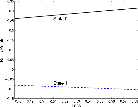
Under baseline parameter values, we have that
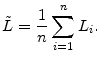
in the tail of the loss distribution. The gaps between finite portfolio and asymptotic conditional probabilities of default and migration are plotted in Figure 10 in the neighborhood of the asymptotic
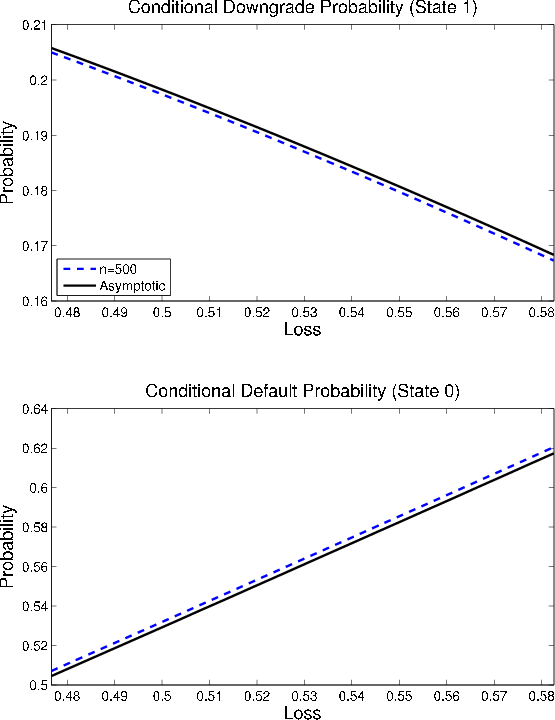
Now consider that the conditional downgrade probability is decreasing in ![]() in the tail of the loss distribution, as we see in the upper panel of Figure 11. As noted earlier, this is because the conditional default probability (plotted in the lower panel) "steals" mass from the conditional downgrade probability at extreme levels of loss. Thus, we have
in the tail of the loss distribution, as we see in the upper panel of Figure 11. As noted earlier, this is because the conditional default probability (plotted in the lower panel) "steals" mass from the conditional downgrade probability at extreme levels of loss. Thus, we have
Conclusion
Granularity adjustment is useful as a gauge of how well a bank has diversified idiosyncratic risk. The results of this paper ease the way for application of the GA methodology to the mark-to-market models that are favored by more sophisticated financial institutions. We have demonstrated that the GA is analytically tractable for a large class of mark-to-market models of portfolio credit risk. This class is restrictive in imposing a single systematic factor, but in other respects is much more general than the models observed in practical application. In particular, we allow in our analysis for spreads at the horizon to depend on the realization of the systematic factor.
We derive explicit expressions for the GA for CreditMetrics and KMV Portfolio Manager. As an application, we explore the comparative statics of the GA in CreditMetrics, and find relationships that are sometimes non-monotonic and sometimes counterintuitive. In particular, we observe that the
comparative statics for the GA with respect to transition probabilities, maturity, and the market risk premium are essentially mirror images of the corresponding comparative statics for asymptotic
![]() . We have argued that this phenomenon has a single explanation: The presence of idiosyncratic risk in the finite portfolio implies that a tail loss event need
not be ascribed exclusively to an unfavorable tail realization of
. We have argued that this phenomenon has a single explanation: The presence of idiosyncratic risk in the finite portfolio implies that a tail loss event need
not be ascribed exclusively to an unfavorable tail realization of ![]() . Rather, extreme losses in the finite portfolio case are most likely to be generated by a combination of unfavorable
systematic and idiosyncratic draws. Default events induce larger loss than downgrades, so the idiosyncratic effect will manifest as a higher than conditionally expected default rate. This implies that VaR is more sensitive to default risk and less sensitive to migration risk than asymptotic
. Rather, extreme losses in the finite portfolio case are most likely to be generated by a combination of unfavorable
systematic and idiosyncratic draws. Default events induce larger loss than downgrades, so the idiosyncratic effect will manifest as a higher than conditionally expected default rate. This implies that VaR is more sensitive to default risk and less sensitive to migration risk than asymptotic
![]() . As the GA is the difference between VaR and
. As the GA is the difference between VaR and
![]() , the comparative statics for the GA with respect to migration risk parameters must be opposite in sign to the corresponding comparative statics for asymptotic
, the comparative statics for the GA with respect to migration risk parameters must be opposite in sign to the corresponding comparative statics for asymptotic
![]() .
.
In the absence of an analytical expression for the GA, this phenomenon would have been difficult to uncover. Estimation of the GA by simulation is difficult enough, because simulation noise tends to swamp the small gap between VaR and asymptotic
![]() . Clean simulation-based estimates of the comparative statics would have been even more challenging.
. Clean simulation-based estimates of the comparative statics would have been even more challenging.
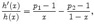
A. Parameter restrictions in the beta-trinomial model
In this appendix, we obtain parameter restrictions sufficient to guarantee that asymptotic
![]() will increase with the state return parameters. The necessary and sufficient condition for
will increase with the state return parameters. The necessary and sufficient condition for
![]() to increase with
to increase with
![]() is
is
For
For the downgrade state (![]() ), the left and right hand sides of condition (24) are non-monotonic, i.e.,
), the left and right hand sides of condition (24) are non-monotonic, i.e.,
 |
 |
 |
 |