The Housing Crisis and State and Local Government Tax Revenue: Five Channels
Keywords: Property tax, sales tax, state income tax, transfer tax, housing market
Abstract:
This paper was reposted in October 2010 to update values in table 3.
JEL Codes: R1; R21; R50; H20; H71
I. Introduction
The housing market contraction of the past four years was the largest since the Great Depression, and it arguably played an important role in the ensuing downturn in economic activity. State and local tax revenues have suffered considerably during this episode. In this paper we seek to disentangle the impact of the housing market downturn on state and local tax revenues from the broader impact of the economic recession.
The housing market influences state and local tax revenues in many ways. We focus on five channels that we argue are the most important. The first two channels, the property tax and the real estate transfer tax, are a direct function of the value of real estate and the volume of real estate transactions. The third and fourth channels involve the sales tax. Sales of materials used in new construction and the renovation of existing structures directly affect sales tax revenues. We also consider an indirect effect on sales tax revenues related to general household expenditures: if changes in housing wealth affect homeowners' consumption, then a large drop in real estate values can reduce the sales tax revenues from all types of goods and services. Finally, personal income tax revenues will be affected by the reduction in employment related to construction and real estate activity. A few of these channels incorporate commercial as well as residential real estate, but in most cases data limitations prevent us from examining the commercial real estate market directly.
Our main purpose is to provide national estimates of the impact of each channel by aggregating across all states and localities. State and local governments exhibit significant heterogeneity in their tax systems, so the impact of each channel will clearly vary across locations (e.g. for a given fall in home sales, a state with a greater reliance on real estate transfer tax revenues will see a larger fall in total tax revenue than a less reliant state). Nevertheless, it is informative to estimate the overall national impact of each of the five channels because it reveals the effect on the average state or local government. Moreover, aggregate data on tax revenues are available on a much more-timely basis than detailed tax data for individual state and local governments, allowing for a better assessment of the current condition of tax revenues. The national estimates also provide a baseline from which to view the experiences of individual states and localities. This baseline is particularly useful in preventing the natural tendency to extrapolate from the most visible-typically the most negative - experiences to the nation as a whole. After presenting our national estimates, we examine the heterogeneity across governments by performing simulations for each state, based on the national estimates and the individual parameters of each state's tax system.
Our analysis can be broken into two primary components. The first component focuses on the property tax channel, which is the primary source of tax revenue in most localities. Perhaps surprisingly, property tax receipts continued to grow at a robust pace through the end of 2009, even though house values had plunged in the previous three years. We ask why the property tax has been so resilient to these house price declines, and examine whether this resilience is likely to continue. We conclude that the resilience to date is a function of significant lags in the effect of changes in the market value of property on changes in taxable assessments, as well as of the propensity of local policy makers to offset declines in property values by increasing the property tax rate. Analysis of historical data and case studies of the current situation in individual states suggest that, on average, it is unlikely that property tax revenues will fall sharply in the near future.
The second component of the analysis seeks to assess the extent to which the housing market downturn has contributed to the plunge in state revenues through the four other channels. Revenues from some of these sources have contracted sharply in the past several years, but the contributions to
the decline in total state tax revenues are relatively modest. We estimate that the four channels reduced total state tax revenues by only $15 billion (in year 2005 dollars) from 2005 to 2009, a relatively small fraction of the $650 billion in state tax revenues in (fiscal year) 2005. Although a
net decline of this magnitude is by no means trivial, it is only
![]() of the standard deviation of changes in annual total state tax revenues from 1990 to 2005, and it
was spread out over four years. However, the drop in revenue was more severe in some states. For example, we estimate that total state tax revenues in Florida were reduced by $5.6 billion, or 14 percent of its 2005 tax revenues. By contrast, housing-related revenues in a number of states did not
fall much at all between 2005 and 2009. Much of the drop in housing related revenues from 2005 to 2009 is due to the transfer tax and sales tax channels.
of the standard deviation of changes in annual total state tax revenues from 1990 to 2005, and it
was spread out over four years. However, the drop in revenue was more severe in some states. For example, we estimate that total state tax revenues in Florida were reduced by $5.6 billion, or 14 percent of its 2005 tax revenues. By contrast, housing-related revenues in a number of states did not
fall much at all between 2005 and 2009. Much of the drop in housing related revenues from 2005 to 2009 is due to the transfer tax and sales tax channels.
Because 2005 marked the peak of a strong housing market boom, comparing 2009 to 2005 might exaggerate the negative effect on tax revenues. Therefore, we also compare state tax revenues in 2009 to their predicted level had housing market variables continued to increase at their 1995-2002 trends, instead of first booming and then contracting. We estimate that state tax revenues in 2009 were $31 billion lower than predicted, which is equivalent to 5 percent of the actual state tax revenues in 2009. In this case, all four channels make notable contributions to the deficit between actual and predicted revenues.
While our intent is to quantify the main channels through which the housing market affects state and local tax revenues, it is important to point out that our methods do not identify the causal effect of exogenous house price declines on state and local tax revenues. We attribute all fluctuations in economic activity in housing-related sectors to the housing market, even though the recession likely intensified the depth of the housing market downturn. Furthermore, our methods do not capture effects that occur through the housing market's impact on other sectors, such as on employment in non-housing industries (e.g. retail sales workers at Home Depot). Despite these issues, this is the first paper to provide a rough sense of the overall magnitude and importance of the housing-related components of state and local tax revenues.
II. Background Information
Housing Market
According to many different measures, the housing market expansion and contraction of the past eight years has been the most severe in the post-War period. House prices rose by 64 percent in the four years prior to their peak in 2006:Q1 and then plunged by nearly 30 percent in the subsequent four years. Existing home sales rose by 34 percent in the four years prior to their peak (in 2005:Q3) and then fell by 36 percent. The supply of housing also exhibited large swings: the number of new housing starts rose 24 percent in the four years prior to their peak before falling by 75 percent since then.
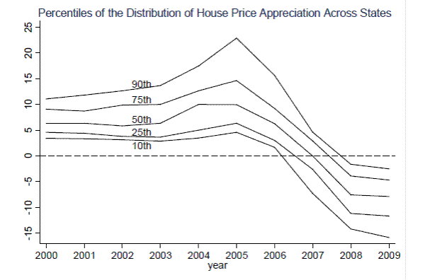
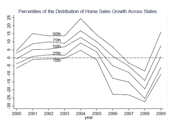
Although the severity of the housing market cycle varied across locations, most states experienced a noticeable swing. The top panel of Figure 1 shows the 10![]() , 25
, 25![]() , 50
, 50![]() , 75
, 75![]() and 90
and 90![]() percentiles of distribution of annual changes in house prices across states (the source of the data will be discussed later). House price
appreciation increased from 2002 to 2005 even at the 10
percentiles of distribution of annual changes in house prices across states (the source of the data will be discussed later). House price
appreciation increased from 2002 to 2005 even at the 10![]() percentile, and house prices fell in all but a few states in 2008 and 2009. The bottom panel shows a similar chart for the
distribution of changes in existing home sales across states.
percentile, and house prices fell in all but a few states in 2008 and 2009. The bottom panel shows a similar chart for the
distribution of changes in existing home sales across states.
State and Local Tax Revenue
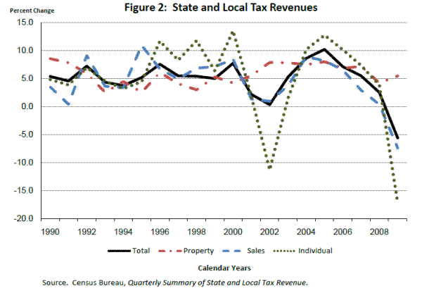
Total state and local tax revenues have been hit hard during the recession.2 As shown in Figure 2, nominal state and local tax revenues fell by almost 5
![]() percent in 2009 after slowing markedly in 2008. 2009 marked the first year that state and local tax
revenues had fallen in nominal terms since the Great Depression, and only the third year since then that revenues did not increase by at least 2 percent (the other two years were 2002 and 2008). The decline in 2009 is attributable to two primary state taxes-the personal income tax and the sales
tax. Income tax revenue plunged 17 percent in 2009, reflecting falling wage and salary income as well as a decline in capital gains realizations. Sales tax revenue fell by 7
percent in 2009 after slowing markedly in 2008. 2009 marked the first year that state and local tax
revenues had fallen in nominal terms since the Great Depression, and only the third year since then that revenues did not increase by at least 2 percent (the other two years were 2002 and 2008). The decline in 2009 is attributable to two primary state taxes-the personal income tax and the sales
tax. Income tax revenue plunged 17 percent in 2009, reflecting falling wage and salary income as well as a decline in capital gains realizations. Sales tax revenue fell by 7
![]() percent due to a decline in retail sales.
percent due to a decline in retail sales.
In contrast, property tax receipts-the primary source of local tax revenues-have held up remarkably well as they grew about 5 percent in both 2008 and 2009. Property tax receipts were the sole source of strength in state and local tax revenue in 2008 and 2009 and have significantly buffered the
decline in other tax sources: Had property taxes been flat in 2009, the decline in overall tax revenue would have been 7
![]() percent instead of 5
percent instead of 5
![]() -a 30 percent more severe tax revenue slump.
-a 30 percent more severe tax revenue slump.
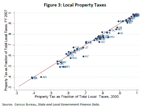
As is visible in Figure 2, property tax revenues generally tend to be less volatile than other forms of tax revenue. The stability of the property tax can also be seen in Figure 3 which plots the local government property tax share-the percent of total local taxes accounted for by the property tax-in 2000 against the share in 2007 (the last available year) by state. The points are clustered along the 45-degree line, illustrating that despite the historic increase in house prices, the property tax share held essentially constant in all states. This stability has long been seen as one of the primary virtues of the property tax (Brunori 2003; Giertz 2006). The magnitude of the collapse in the housing market, however, raises the possibility that property tax revenues might fall. In the analysis below we explain why revenues had not yet fallen through the end of 2009 and we assess the likelihood that they will fall in the near future.
III. Results: Property Tax
This section examines the resilience of the property tax in the face of the steep home price declines of the last several years. First, drawing on Lutz (2008) we discuss the relationship between house price changes and property tax revenues. The discussion is important because Lutz's results motivate the analytic approach taken in this paper. Second, we assess the impact of house price declines on property tax collections using state-level panel data. Finally, because the historical data may have limited relevance for the current extraordinary situation in the housing market, we conduct case studies of recent changes in property tax revenues in eight states, including states such as Arizona, California, Florida, and Nevada that experienced unusually large declines in house prices.
The Historical Relationship between Real Estate Prices and Property Tax Collections
Property taxes are by far the most important tax at the local level, accounting for around three-fourths of local government tax revenue. The tax is assessed on the value of residential real property (i.e. personal real estate), commercial, business and farm real property, and personal property (e.g. automobiles). Residential real property accounts for approximately 60 percent of taxable assessments and is the largest component of the tax base by a significant margin; commercial, industrial and farm property account for around 30 percent and personal property accounts for less than 10 percent.3
Abstracting from the significant heterogeneity across jurisdictions, property tax revenue can be defined as being equal to the effective tax rate times the market value of property
where
| (2) | ||||
| mechanical | policy offset |
Lutz (2008) explores two aspects of this relationship. First, he assesses the magnitude of the change in property tax revenues produced by a change in house prices. This analysis sheds light on the average magnitude of the policy offset. If there is no policy offset, then the elasticity of property tax revenue with respect to house prices will equal 1, and if there is complete policy offset, the elasticity will equal 0. Second, he examines the timing of the relationship between house price appreciation and property tax revenue.
Using both time-series data and micro-level panel data from individual governments, Lutz (2008) concludes that the elasticity of property tax revenue with respect to home prices equals 0.4, indicating that policy makers tend to offset 60 percent of house price changes by moving the effective tax rate in the opposite direction of the house price change. The effect of house price changes on property taxes does not occur on average until three years following the change in house prices. This extensive lag likely reflects three institutional features of the property tax. First, the property tax is assessed in a backward looking manner, as the current year's taxes are based on the assessed value of property in the previous year. Second, assessed values often lag market values. In some cases this lag is by design or legal mandate and in others it is due to "poor" administration. Poor administration may sometimes be intentional, particularly in jurisdictions which elect their tax assessor.5 Third, most states have some form of cap and/or limit on increases in property tax rates, tax revenues or taxable assessments. During periods of rapid house price growth, these limits will prevent assessments or revenues from growing at the same pace as market values. Thus, a `stock' of untaxed appreciation will develop. Assessments will catch-up to market values only when house price growth slows below the limit and the `stock' of untaxed appreciation is incorporated into taxable assessments.
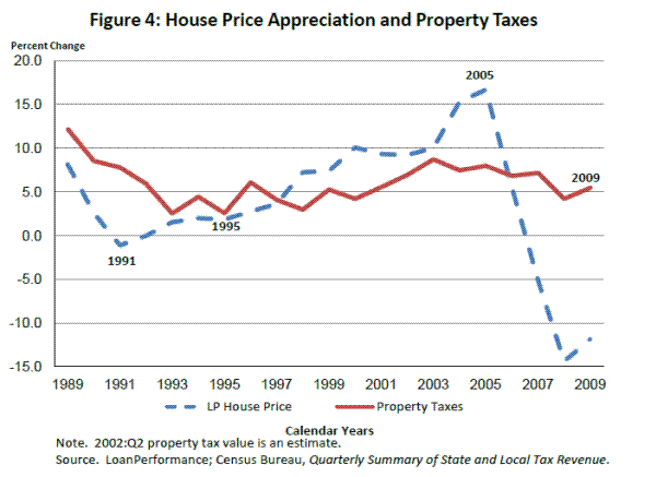
Both aspects of the relationship-the elasticity and the lag-are visible in Figure 4, which displays the annual growth rate of property tax revenue and house values from 1989 to 2009. Focusing first on the lag, the growth rate of both series declined in the early 1990s. Although house price appreciation reached a trough in 1991, property tax revenue growth did not bottom out until 1995, implying that property taxes track real estate prices with a considerable lag. Similarly, in the more recent period, house price appreciation collapsed from 2006 to 2008, but the growth in property taxes barely slowed. Turning to the elasticity, the growth rate of property tax revenues increased at a much slower pace than that of house price appreciation from the mid-1990s to 2005. This observation is consistent with the notion that policy makers tend to offset changes in house prices by adjusting tax rates.
Most relevant for this paper, Lutz (2008) estimates a much smaller relationship between house price declines (as opposed to the typical change in house prices, which is positive) and property taxes. These estimates have limitations in regards to assessing the current situation because the typical house price decline in the sample used in Lutz (2008) is quite small relative to the declines which have occurred over the last several years. Nevertheless, the results strongly suggest that policy makers buffer negative house price shocks by raising property tax rates. Although the magnitude of the response varies greatly from specification to specification, in most cases it is not possible to reject the hypothesis that house price declines have no effect on property tax revenues. Updated results from Lutz (2008) (unreported) that add several more years of data to the sample produce no substantive change in the conclusions.
State-level Panel Data Evidence
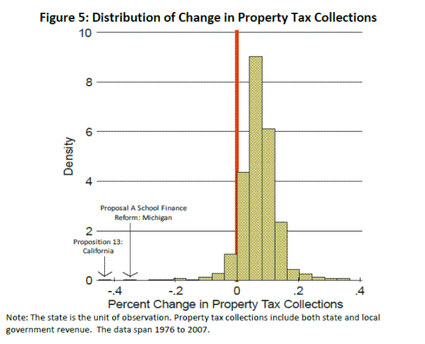
Since the standard econometric approach used in Lutz (2008) failed to find an effect of house price declines on property taxes, we present an analysis that focuses explicitly on episodes of falling house prices using annual state-level panel data on total property tax collections from 1976 to 2007 (including both state and local government collections).6 Figure 5 displays the distribution of the annual percent change in property tax receipts over this period. Declines in property tax collections are rare-only 7 percent of the distribution falls below 0. Furthermore, large declines are extremely rare. Only half of one percent of the annual changes in property tax collections since 1976 exceed negative 15 percent. Many of these extremely large declines are associated with policy changes, such as Proposition 13 in California, that are not directly related to fluctuations in home values. Less than one percent of the declines exceed 10 percent and less than two percent exceed 5 percent.
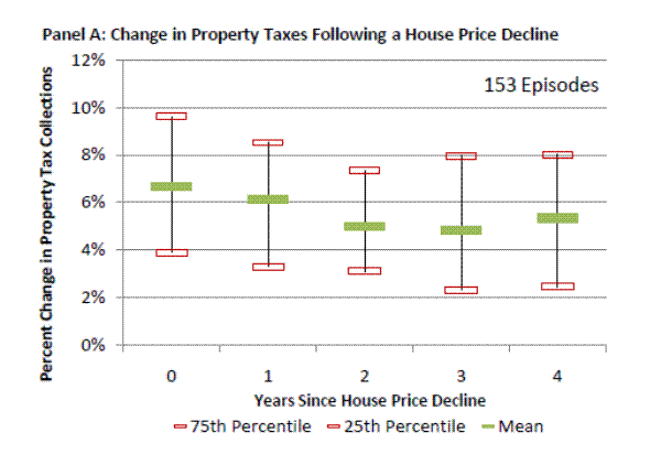
Using an event study framework, Figure 6 plots the distribution of changes in property tax revenues in the year of a decrease in home prices and the four subsequent years. We restrict the sample to the state-year combinations for which property tax data are available for all five years displayed. This restriction ensures that the evolution of the distribution of price changes does not reflect changes in the sample composition. We measure house prices using repeat-sales indexes computed by LoanPerformance, a division of First American CoreLogic. These indexes are similar to those published by the Federal Housing Finance Agency (FHFA), but unlike the FHFA they include homes financed with non-conforming loans and cash. The indexes are based on transactions of single-family homes, condos, coops, foreclosed properties, and short sales. We take annual averages of the monthly index for each state.
We view this analysis as heavily tilted toward finding an effect of house price declines on property tax revenues. Most episodes of house price declines are associated with events that would tend to depress demand for public goods, and hence for tax collections, independently of the change in home prices. For instance, an adverse shock to an industry with a major presence in a state would reduce incomes and cause out-migration, simultaneously reducing the demand for public spending and house prices. We do not account for this omitted variable bias, which should cause us to overstate the positive correlation between house prices and tax revenues. Furthermore, the sample size is quite small. As a result, we do not compute standard errors around the moments of the distribution.
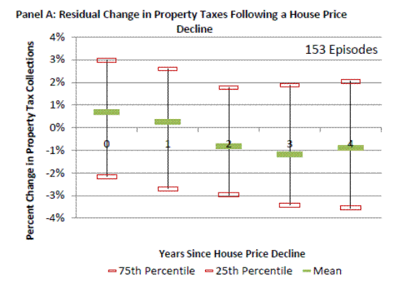
Panel A of Figure 6 displays the event study results using all episodes of house price declines in the sample (of which there are 153 with a mean decline of around 3 percent). The horizontal axis indexes the year relative to the house price decline. For example, year 0 denotes the year of the
decline and year 1 denotes the year following the decline.7 The vertical axis displays the average, 25![]() percentile and 75
percentile and 75![]() percentile of the percent change in property tax revenues in that year. In the year of a house price decline,
property taxes rose by an average of 6
percentile of the percent change in property tax revenues in that year. In the year of a house price decline,
property taxes rose by an average of 6
![]() percent- quite close to the mean change for the sample as a whole (i.e. including years in which
houses prices both increase and decrease). The pace of growth slows only slightly in the two years following the house price decrease and then stabilizes by the third year at around 5 percent. States at the 25
percent- quite close to the mean change for the sample as a whole (i.e. including years in which
houses prices both increase and decrease). The pace of growth slows only slightly in the two years following the house price decrease and then stabilizes by the third year at around 5 percent. States at the 25![]() percentile experienced an increase in property taxes of around 2
percentile experienced an increase in property taxes of around 2
![]() percent, and even the 10
percent, and even the 10![]() percentile (not shown) is greater than zero. House price decreases may slow the pace of property tax growth a bit, but the magnitude of the impact is small and there is absolutely no evidence that house price declines produce a fall in property tax receipts.
These results are especially striking given the positive correlation between house prices and tax revenues that should exist for other reasons (discussed above).
percentile (not shown) is greater than zero. House price decreases may slow the pace of property tax growth a bit, but the magnitude of the impact is small and there is absolutely no evidence that house price declines produce a fall in property tax receipts.
These results are especially striking given the positive correlation between house prices and tax revenues that should exist for other reasons (discussed above).
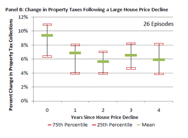
Panel B performs the same exercise, but limits the sample to episodes where house prices fell by more than 5 percent. The sample becomes somewhat thin, as there are only 26 cases when house prices declined by this amount (the mean decline in this subsample is 7.2 percent). In the year of a large house price decline, property tax collections rose by a robust 10%. This strong increase may reflect rapid house price appreciation in the years preceding large declines in prices. Although property tax growth fell by roughly 3 percentage points in the year following the house price decline, tax collections continued to expand at the healthy pace of around 6 percent.
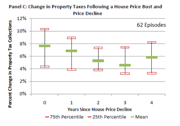
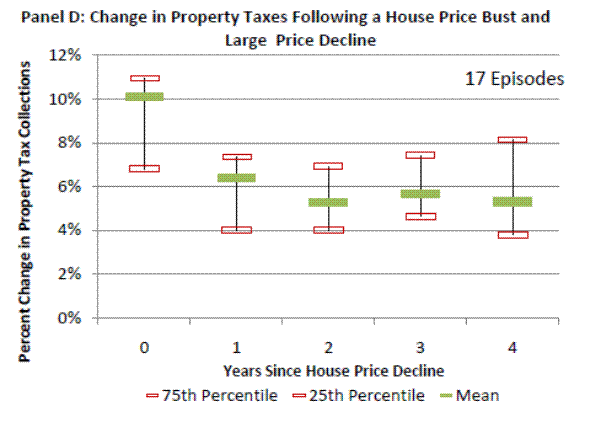
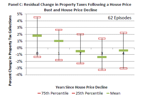
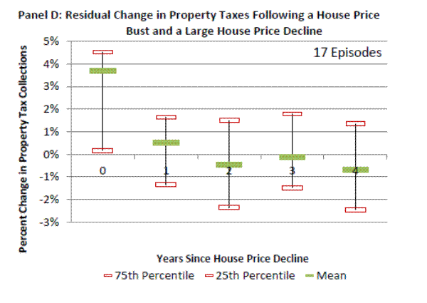
Panel C limits the sample to episodes of house price declines which can be categorized as "busts." Carlson (2010) defines a housing bust as a period in which the change in house prices is significantly below what would be predicted by fundamentals such as personal income, the unemployment rate, and mortgage rates for five consecutive quarters.8 The sample contains 62 such "busts" that also involved a decline in house prices (a bust may occur when prices continue to rise, but at a slower pace than predicted by fundamentals). These bust episodes are arguably more relevant to current housing market conditions than typical house price declines. The pace at which property tax receipts grow tails off somewhat following house price busts, but the magnitude of this deceleration is not large and receipts continue to rise at a reasonably-rapid pace. Since some "busts" occur even when house prices fall only modestly, Panel D restricts the sample to busts in which house prices fell in excess of 10 percent. These busts are associated with a drop in the growth of tax collections of around 4 percentage points, but growth remains relatively strong.
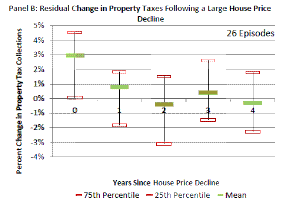
Figure 7 is similar to Figure 6 but attempts to control for a few things that are correlated with house prices and property tax revenues. First we regress growth in property tax collections on a state-specific constant and contemporaneous and lagged population growth. The state-specific constant controls for long-term differences in the rate at which tax revenues increase across states, while population growth is a very rough control for the demand for public goods. The regression is estimated over the entire sample (i.e. not just the portion of the sample with house price decreases). Then we plot the residuals in the years following house price declines and/or busts. The sample mean of the residual is 0 by construction.
The residuals provide even less evidence that house price declines significantly reduce property tax collections. House price declines are associated with an eventual slowing in the residual growth rate of tax collections, but the magnitudes are quite small, typically 1 percentage point or less. Although residual declines of 2 to 3 percent are not uncommon, these magnitudes are still smaller than average growth in property tax collections. Calculating the residuals based on a larger set of covariates (results unreported) tends to further reduce the magnitude of the effect.
Contemporaneous Case Studies
Case studies of individual states in recent years provide direct evidence on why property tax collections have held up so well through the end of 2009. This analysis is also useful because the historical data used in the prior two sections may be of limited relevance to the current situation. Furthermore, it provides insight into the possibility that property taxes may start falling in the near future in a very delayed response to the drop in house prices. The case studies use data collected from individual state sources such as departments of taxation.9
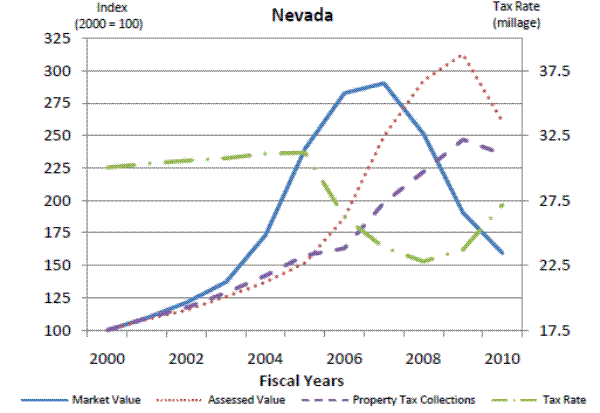
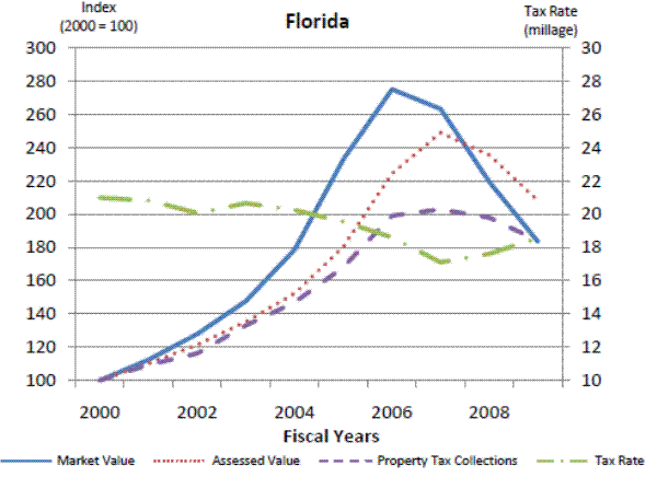
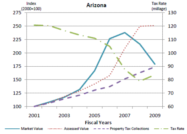
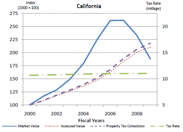
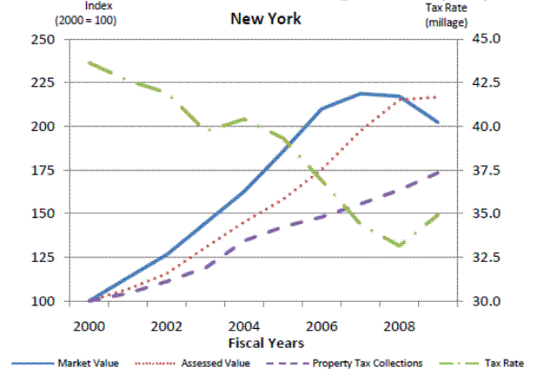
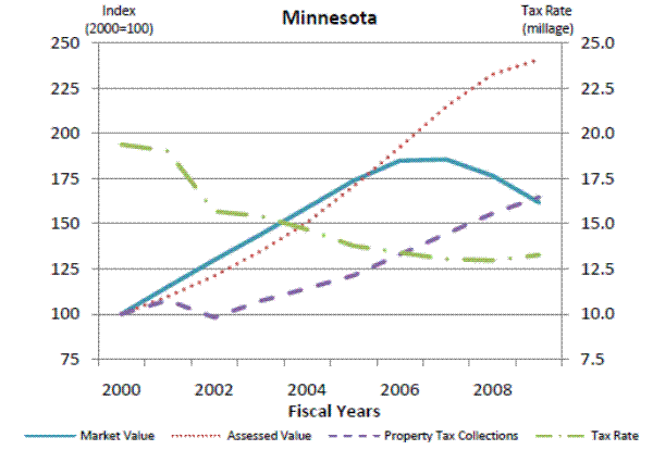
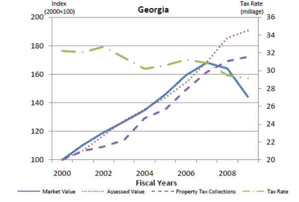
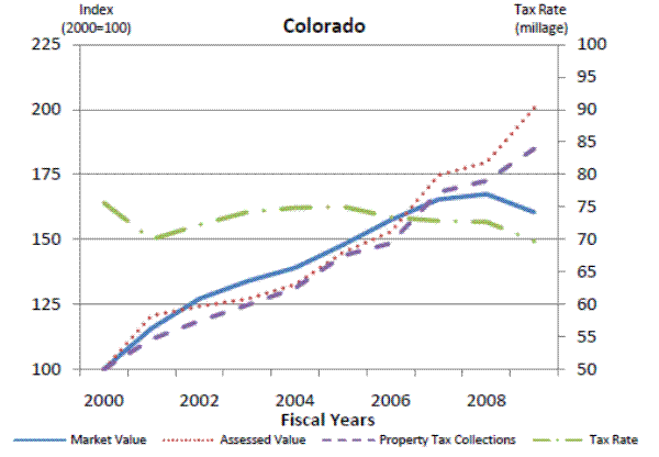
Figure 8 presents the cases studies graphically. For each state there are four time-series, the first three of which are indexed to equal 100 in 2000. The first series is the market value of residential real estate based on the Loan Performance house price indexes and, to account for changes in the stock of housing, on the Census Bureau's housing unit estimates. The second series is the assessed value of all real estate, collected from individual state sources. To the extent possible, this value captures the aggregate taxable value of real estate (e.g. the value of exemptions is removed from the total). The third series is total property tax collections, also from state sources. The final series is the property tax rate, defined as total collections divided by aggregate assessed value (right axis). We call this tax rate the "average assessed tax rate" to avoid confusion with the "effective tax rate," which we define as based on market values rather than assessed values. All series are shown for fiscal years with the specific years displayed for a given state reflecting data availability.
Our first four case studies examine the four states with the most extreme housing market cycles. Starting with Nevada, the market value of real estate soared from 2000 to 2006 and fell sharply starting in 2008.![]() Assessed values appear to lag market values by at least two years and only began to turn down in 2010. The assessed tax rate held roughly steady until 2006 when it began to fall with the introduction of a tax abatement program. It then reversed course in 2009 as
the growth in assessed values slowed and turned sharply upward in 2010 as assessed values began to plunge. Combining the evolution of assessed values and tax rates, property tax revenues rose by 6 percent from 2008 to 2010 even though the market value of real estate collapsed by almost 40 percent
during this period. Thus, the lags in assessed values and offsetting movements in the tax rate substantially muted the impact of the housing downturn on tax revenues in Nevada. Although tax revenues did fall by 4
Assessed values appear to lag market values by at least two years and only began to turn down in 2010. The assessed tax rate held roughly steady until 2006 when it began to fall with the introduction of a tax abatement program. It then reversed course in 2009 as
the growth in assessed values slowed and turned sharply upward in 2010 as assessed values began to plunge. Combining the evolution of assessed values and tax rates, property tax revenues rose by 6 percent from 2008 to 2010 even though the market value of real estate collapsed by almost 40 percent
during this period. Thus, the lags in assessed values and offsetting movements in the tax rate substantially muted the impact of the housing downturn on tax revenues in Nevada. Although tax revenues did fall by 4
![]() percent in 2010, it seems that the willingness of policy makers to adjust tax rates will make the
ultimate effect of the housing downturn on tax revenues much smaller than suggested by a straight read of the decline in the market price of housing.
percent in 2010, it seems that the willingness of policy makers to adjust tax rates will make the
ultimate effect of the housing downturn on tax revenues much smaller than suggested by a straight read of the decline in the market price of housing.
Our next two case studies examine Florida and Arizona. In Florida, house prices more than doubled from 2000 to 2006. Assessed values did not increase as fast as house prices and the assessed tax rate declined during this period, which caused property tax revenues to rise at a much slower pace than house prices. The assessed tax rate began increasing in 2008 as assessed values began falling, again working to blunt the impact of the housing market contraction on tax collections. Arizona displays trends broadly similar to Nevada and Florida. House prices soared and then collapsed, with assessed values lagging the movement in market values. The assessed tax rate moved upward with the decline in market values in 2009, buffering the impact of the housing market on tax collections.
The next case study is California. Although the trajectory of housing prices is similar to Arizona, Florida, and Nevada, local governments in California face a different set of challenges because of Proposition 13. Approved by voters in the late 1970s, Proposition 13 dictates that assessed values cannot grow by more than 2 percent per year or the inflation rate, whichever is smaller, unless the house is sold and the assessed value is reset to the market value. Proposition 13 also limits property taxes not to exceed 1 percent of the assessed value. As expected, Figure 8 shows that the assessed tax rate held constant at about 1 percent. Due to this constant rate, growth in property tax collections mirrors that of assessed values, which continued to climb even after house prices fell sharply after 2007. Because Proposition 13 has created a large wedge between market values and assessed values, it will likely take a very long time for assessed values to catch up with market values. If that does occur, the legislated cap on the tax rate would cause property tax revenues to fall.
Our next four case studies consider states with less pronounced movements in the housing market than Arizona, California, Florida, and Nevada. New York is the first; it is a more typical state than the previous case studies because it experienced a housing cycle similar to the national average and it does not have stringent property tax limitations. Figure 8 shows that assessed values lagged house prices, as they continued to rise through 2008 and only flattened out in 2009. Property tax revenues rose more slowly than assessed values over the decade because the assessed tax rate trended down. In 2009, the assessed tax rate increased notably which contributed to an increase in property tax revenues of 6 percent.
Our final three cases studies consider Minnesota, Georgia, and Colorado, which are meant to reflect other types of housing market experiences. Unlike the previous case studies, assessed values and market values rose at the same pace during the upswing in the housing market in these states. Once the downturn took hold, though, assessed and market values diverged sharply, with assessed values continuing to rise even as market values fell. Thus, in these states as well property tax revenues to-date have been buffered from the drop in house values. Although assessed tax rates did not increase in these states, an apparent lag between assessed and market values has likely allowed property tax revenues to diverge from the market value of housing.
Taken together, the cases studies shown in Figure 8 reveal a number of facts about the impact of the current housing downturn on state and local property tax revenues. First, there is a significant amount of heterogeneity across states in their experience of the housing cycle, the institutional features of their property tax assessment and collection practice, and their responses to the housing downturn. Second, assessed values lag market values in many states, which helps to support property tax revenues when house prices fall. This support is particularly useful because state and local governments usually face sharp declines in other tax revenues when house prices fall (due to deteriorating economic conditions). Third, when assessed values do catch up with market values, local officials appear to be willing to at least partially offset the decreases in assessed values with increases in tax rates. However, continuing to offset price declines by raising tax rates may eventually become politically impossible (Bennett and Perry 2009, Wiseman 2010). Overall, though, we read the evidence from the historical data and the case studies as suggesting it is quite unlikely that property tax collections will fall steeply in the next few years. Even if property taxes do decline by a large amount, the significant lag between this event and the housing market downturn will have provided the state and local government sector time to at least partially recover from the plunge in other revenue sources (Figure 2).
IV. Results: Four Non-Property Tax Channels
Simulation Approach for Remaining Four Channels
In the remainder of the paper, we assess the impact of the housing market downturn on other forms of tax revenue: transfer taxes, sales taxes on construction materials, sales taxes on other goods and services, and personal income taxes. For each channel we quantify the effect in two ways. First, we calculate the drop in tax revenue in real terms from 2005-the peak of the housing market-to 2009.10 Specifically, we calculate the change in the relevant housing-related tax base from 2005 to 2009 for each state (e.g. for the transfer tax effect the tax base is the number of real estate transactions). We then estimate the implied change in tax revenue arising from the change in the base using state-specific tax rates. We call this effect the "peak year" method because it uses revenues at the (aggregate) housing market peak as a starting point. It could be argued that in 2005 the housing market was out of equilibrium and that quantifying revenue losses relative to such unsustainable levels is problematic. Therefore, we also quantify the effect of the housing market on state revenues relative to state-specific trends, which we call the "trend growth" method. This method involves extrapolating each housing-related tax base using its average growth rate from 1995 to 2002. By comparing the implied counterfactual level of taxes in 2009 to actual tax collections in 2009, we gauge the level of revenue in 2009 relative to a world in which the housing market grew at trend instead of experiencing a boom-bust cycle.
Transfer Taxes
The real estate transfer tax, sometimes referred to as a deed recordation tax or a realty conveyance tax, is collected when real estate changes hands and is typically based on the value of the real property being transferred (Behrens and Gravelle 2004). The tax rate is generally the same for all transfers, although in some instances it is progressive in the sense that the tax rate rises with the value of the transfer. Currently, 37 states and the District of Columbia assess the tax. In 24 states the tax is collected only by the state, in 11 states it is collected by both state and local governments, and in 2 states it is purely a local tax. In 2007, roughly two-thirds of total collections occurred at the state level.
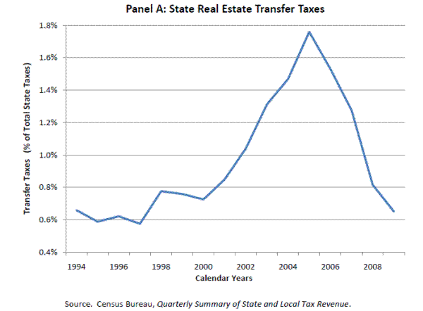
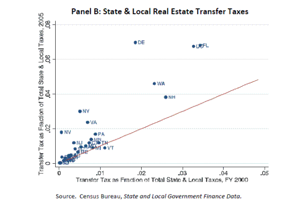
Transfer taxes have typically comprised a negligible share of total state tax revenues. As can be seen in Panel A of Figure 9, transfer taxes were less than 1 percent of total state revenues from 1994 through 2000.11 As the housing market boom got underway, however, the transfer tax share began to grow sharply, reaching a peak of nearly 1.8 percent in 2005 before falling back to around 0.7 percent by 2009. Panel B shows the run-up in the transfer tax share from 2000 to 2005 on a state-by-state basis. The horizontal axis displays the transfer tax as a share of state and local government taxes in fiscal year 2000 and the vertical axis displays the share as in fiscal year 2005 (near the peak of transfer tax collections). Almost all of the states are above the 45 degree line, indicating that the transfer tax grew in importance over this period. The growth was particularly notable in New York, Delaware, Washington state, Washington DC and Florida.
Transfer tax revenues,
T![]() , can be separated into two components: the tax rate,
, can be separated into two components: the tax rate,
![]() , times the value of real estate transactions,
V
, times the value of real estate transactions,
V![]() (which is itself equal to the number of real estate transactions,
N
(which is itself equal to the number of real estate transactions,
N![]() , times the average sales price,
, times the average sales price,
![]() ):
):
| T |
(3) |
Taking logs and first-differencing yields:
| (4) |
| (5) |
Equation (4) makes clear that the elasticity of transfer tax revenues with respect to the value of real estate transactions equals 1:
![]() . Similarly, equation (5) shows that the elasticity of transfer tax revenues with respect to the number of
real estate transaction and the average value of real estate transactions both equal 1:
. Similarly, equation (5) shows that the elasticity of transfer tax revenues with respect to the number of
real estate transaction and the average value of real estate transactions both equal 1:
 |
(6) |
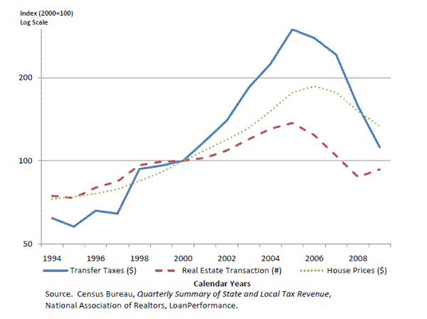
The relationship between transfer tax receipts and the housing market is visible in the aggregate time-series data shown in Figure 10. (The series are indexed to equal 100 in 2000 and a log scale is used) As both the volume of real estate transactions and home prices surged in the first half of the decade, transfer taxes rose 200 percent. Tax receipts then turned downward in 2006 when the volume of real estate transactions began falling. The decrease in collections intensified in 2008 as housing prices began to slide
We estimate the elasticities of transfer tax revenues to real estate transactions and house prices using state-level panel data on annual state government tax collections from 1999 to 2009 and the empirical analogue to equations (4) and (5)
| (7) |
| (8) |
where s indexes states and t indexes year. We measure home sales by taking annual averages of quarterly data published by the National Association of Realtors. These sales include sales of existing single-family homes and condos, but exclude sales of new homes.12 The house price data are the LoanPerformance indexes described above. The transfer tax data are from the Census Bureau's Quarterly Summary of State and Local Government Tax Revenue.
Empirical estimates of each elasticity may fail to equal 1 for a number of reasons. First, in some states the tax rate is progressive, leading to estimates of
![]() greater than 1: as the average value of real estate transactions grows, more transactions will fall into higher tax brackets leading to a higher average
tax rate. Second, the error term in equation (6),
greater than 1: as the average value of real estate transactions grows, more transactions will fall into higher tax brackets leading to a higher average
tax rate. Second, the error term in equation (6),
![]() , incorporates any changes in transfer tax rates,
, incorporates any changes in transfer tax rates,
![]() log
log![]() . If the propensity to change tax rates is correlated with real estate
transaction volumes or prices, the
. If the propensity to change tax rates is correlated with real estate
transaction volumes or prices, the
![]() s will be biased. The sign of the bias will depend upon whether such tax changes work to intensify or dampen the influence of changes in the real estate market on transfer tax
receipts (e.g. if policy makers reduce rates when receipts are growing strongly, there will be a downward bias). Third, although the transfer tax typically applies to both residential and commercial real estate transactions, the housing market measures used here pertain only to the residential side
of the market (commercial measures at the state-level are unavailable). If movements in the commercial market are positively correlated with movements in the residential market, there will be an upward bias. Finally, the state-level real estate variables are almost certainly measured with error
leading to downward attenuation bias.
s will be biased. The sign of the bias will depend upon whether such tax changes work to intensify or dampen the influence of changes in the real estate market on transfer tax
receipts (e.g. if policy makers reduce rates when receipts are growing strongly, there will be a downward bias). Third, although the transfer tax typically applies to both residential and commercial real estate transactions, the housing market measures used here pertain only to the residential side
of the market (commercial measures at the state-level are unavailable). If movements in the commercial market are positively correlated with movements in the residential market, there will be an upward bias. Finally, the state-level real estate variables are almost certainly measured with error
leading to downward attenuation bias.
The estimation results are presented on Table 1. Column (1) reports estimates from equation (6), which constrains the coefficients on real estate volumes and prices to be equal and column (2) presents the results of equation (7), which relaxes this constraint. The coefficient on the value of real estate transactions is close to the expected value of 1 and the 95% confidence interval easily encompasses 1 (column 1). However, the coefficients on the two components of the value of transactions are significantly different from 1 (column 2). The house price coefficient is equal to 1.6, while the home sales volume coefficient is equal to 0.7. It is possible that the house price measure is greater than one because it is correlated with movements in the commercial real estate market.13 At the same time, measurement error in the home sales measure arising from the inability to measure new home sales may reduce the estimated effect of transaction volumes, thereby raising the estimated effect of house prices on transfer taxes. Column (3) drops from the sample the 8 states with progressive transfer tax schedules. As expected, the house price coefficient falls somewhat (although the home sales coefficient falls as well). Finally, column (4) also drops the 12 states that increased their tax rates between 1999 and 2009 (no state reduced its tax rate over this period). The restriction has little impact on the results, suggesting that tax rate changes are not significantly biasing the results.
Using the "peak year" approach, the elasticity estimates from column (4) combined with the state-level home price and sales volume data suggest that total state government transfer tax revenue should have declined by $6
![]() billion (real 2005 dollars) from 2005 to 2009, equal to 53 percent of the 2005 peak in this form of
revenue. The estimate is close to the actual decline of almost $8 billion Using the trend growth approach, we estimate that transfer tax receipts in 2009 were $4
billion (real 2005 dollars) from 2005 to 2009, equal to 53 percent of the 2005 peak in this form of
revenue. The estimate is close to the actual decline of almost $8 billion Using the trend growth approach, we estimate that transfer tax receipts in 2009 were $4
![]() billion lower than they would have been if house prices and transactions volumes had continued to
expand at their 1995-2002 average growth rates
billion lower than they would have been if house prices and transactions volumes had continued to
expand at their 1995-2002 average growth rates
Direct Sales Tax Channel
Builders typically pay either sales tax on construction materials that they purchase or the equivalent use tax if the materials are purchased out of state. When the construction sector shrinks, states lose sales tax revenue from numerous construction inputs ranging from lumber and concrete to durable goods like washing machines. To estimate the sales tax revenue generated by the residential construction industry, we consider sales of materials that are used in new construction and renovation. We estimate the materials input cost of new construction by multiplying the number of new housing units built in each state by the cost of construction materials in that state. Single-family and multifamily housing estimates are calculated separately. We use the number of building permits issued for new housing units (reported by the Census Bureau) to proxy for the number of newly-constructed housing units in each state, and we estimate the cost of construction materials as the cost per square foot of construction materials multiplied by the average square footage of new housing units from the "Characteristics of New Housing" report of the Census Bureau. The square footage data are reported annually for the four Census regions (and separately for single-family and multifamily structures).
We obtain data on single-family materials costs from Residential Cost Data, a publication by R.S. Means, which is a well-known construction cost estimator. For each census region, we determine the cost in 2009 of materials used in an average-quality 2-story house with square footage equal to the average square footage of new housing units in that region. Then we multiply this cost by the average cost index for each state and year, which generates variation both across states and over time.14 R.S. Means does not separate multifamily construction costs into materials and labor costs, so for the multifamily sector we assume that materials are 50 percent of the reported cost of materials and installation.15 The cost of materials and installation is based on the estimated cost of a 3-4 story apartment building, which was the typical height of new multi-family buildings in all 4 census regions in the American Housing Survey.16 As with the single-family costs, we multiply the 2009 cost estimate by the cost indexes for each state and year. Finally, we multiply the state-level estimates of materials costs for new single-family and multifamily units by state-level sales tax rates to obtain sales tax revenues.
Data on residential renovation do not exist annually at the state level. Therefore, we estimate state-level renovation expenditures by multiplying the total number of building permits (for new housing units) issued in the state by the national ratio of spending on residential improvements relative to the aggregate number of building permits. The residential improvement data are nominal expenditures on owner-occupied and rental units based on a combination of estimates from the Census Bureau and the BEA.17 We assume that materials inputs are 1/3 of improvement expenditures in each state.18 As with the materials costs for new construction, we multiply the state-level estimates of renovation materials costs by state-level sales tax rates to obtain sales tax revenues.
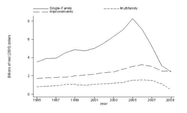
Figure 11 shows our estimates of real sales tax revenues from the materials used in new single-family construction, new multifamily construction, and improvements. The largest component is single-family, which peaked at $8.2 billion in 2005 and had plunged 71 percent by 2009. Multifamily materials inputs show a similarly-large percentage drop during this period, although they make up a much smaller share of total construction materials spending. Our estimates suggest that revenues related to materials used in residential renovation only declined by 17 percent in real terms from 2005 to 2009. Adding these three pieces together and using the peak year method, total state revenues from sales of construction materials fell by 58 percent ($7.4 billion) from 2005 to 2009. Although this decrease is large in percentage terms, it is only 3 percent of the $222 billion dollars in general sales tax revenues generated in 2005.
To evaluate the level of sales tax revenues in 2009 using the trend growth method, we estimate trend expenditures on construction materials for each of the three components (single-family, multi-family, and improvements) assuming that after 2002 the real level of spending continued to increase at its 1995-2002 average growth rate. Then we apply the actual sales tax rate in each state and year to obtain trend sales tax revenues. Summing across all three categories, aggregate sales tax revenues were 68 percent lower ($11.3 billion) in 2009 than they would have been had spending continued at its 1995-2002 trend. Even this seemingly-large gap was only 6 percent of total state sales tax revenues in 2009.
Indirect Sales Tax Channel
Housing is the most important component of wealth for many households. According to the 2007 Survey of Consumer Finances (SCF), housing value accounted for at least half of total assets for 47 percent of households. Booms and busts in the housing market can induce increases and decreases in personal consumption through two channels. The first channel is the conventional wealth effect. Similar to financial assets, increases in house values can raise consumption by increasing the amount of resources available for households. The second channel is through providing collateral against which liquidity-constrained households can borrow. If the current housing downturn has reduced consumption through either of these two channels, it will have reduced the sales tax revenues of state and local governments.
A large number of studies have examined the size of the housing wealth effect using macro and micro data, and the estimates vary significantly from study to study. For example, Case, Quigley, and Shiller (2005) find a large effect of housing wealth on household consumption, but Attanasio, Blow, Hamilton, and Leicester (2009) argue that changes in house prices do not directly influence the spending of homeowners. Cooper (2009) examines the 1996-2005 wave of the Panel Study of Income Dynamics (PSID) and finds a marginal propensity to consume (MPC) of 3.5 cents per dollar increase in housing wealth. Mian and Sufi (2009) use credit report data and estimate a MPC of 25 to 30 cents. Dynan (2010) examines data from the Consumer Expenditure Survey (CE) and finds no link between growth in house prices and growth in homeowners' consumption of nondurable goods. In this paper, we choose a middle ground and assume a MPC of 3 cents for every dollar increase in housing wealth. We allow the housing wealth effect to phase-in over three years: 60 percent in the first year, 90 percent in the second year, and 100 percent in the third year.
To estimate the housing wealth effect on state tax revenues, we assemble data on house prices, housing units, state sales tax rates, state sales tax exemptions of grocery food and clothes, and expenditure fractions of grocery food and clothes. We obtain 1995-2009 state-level total housing wealth by inflating the aggregate value of housing in each state from the 2000 Census with the real house price appreciation rate suggested by the Loan Performance house price indexes and the change in the Census Bureau's estimates of the number of housing units in each state. The 1995-2009 state sales tax rate data are from the State Tax Handbook. In many states, grocery food and clothes are exempt from sales taxes. As a result, the changes in the consumption of grocery food and clothes will not affect sales tax revenues in these states. We obtain data on whether each state exempts grocery food or clothes from the 2008 State Tax Handbook and we estimate that on average grocery food and clothes account for 7.4 and 3.6 percent of total consumption, respectively, using the 2008 CE data. We calculate the housing wealth effect by multiplying the aggregate value of housing in a state by the MPC out of housing wealth, adjusting the resulting consumption estimates for grocery food and clothing expenditures in states where these expenditures are not taxed, and then multiplying the result by the state sales tax rate.
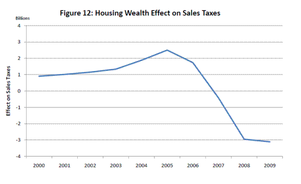
Figure 12 shows our estimates of the housing wealth effect on state sales tax revenues from 2000 to 2009. House prices and construction activity increased in the late 1990s and early 2000s, boosting state sales taxes through the housing wealth effect. As the housing boom accelerated from 2003 to 2005, our estimate of the indirect sales tax effect also surged (from about $1.3 billion to $2.5 billion). House prices began to decline in 2006. However, aggregate housing wealth continued to expand due to continued inflows from new construction. Housing wealth started to fall in 2007, and we estimate that housing wealth-related sales tax revenues fell significantly in 2008 and 2009.
We estimate that sales tax revenue generated by housing wealth declined by $4.8 billion from 2005 to 2009. To carry out the "trend growth" simulation, we predict real house prices and the number of housing units based on their average growth rates from 1995 to 2002. In this counterfactual, state sales tax revenues induced by housing wealth continue to grow steadily from 2003 to 2009. Actual housing wealth-related sales tax revenues in 2009 were $6.1 billion lower than revenues predicted by these trends.
Personal Income Tax Channel
The housing downturn has reduced labor income in housing-related industries. We assess the impact of these declines on personal income tax receipts at the state level by focusing on two housing-related industries: construction (NAICS 23000) and real estate (NAICS 53100). The construction industry includes residential and nonresidential construction of buildings, heavy and civil engineering construction, and specialty trade contractors.19 The real estate industry includes real estate agents and brokers, lessors of real estate, property managers, and appraisers. It does not include mortgage brokers, who cannot be separated out from the other workers in the credit intermediation category in the state-level data.
For each sector, we calculate the average wage per job by state from the BEA's Regional Economic Accounts. Both full-time and part-time workers are included in these estimates. Wage and salary disbursements include commissions, tips, bonuses, and voluntary contributions to deferred compensation plans, but do not include the employers' contributions to pension and insurance funds or to social insurance. They are based primarily on state unemployment insurance records. The 2009 data are not yet available, so we assume that the growth rate of the average wage from 2008 to 2009 is the same as the growth rate of average weekly earnings in that industry from the BLS's Current Employment Statistics.20 Using the NBER's Taxsim module, we estimate the total state income tax payments that would be paid by an individual earning the average wage in that state and industry. We assume that the individual has no non-wage income, is married, has two children, and that the spouse's labor income is 70 percent of construction workers' income and 80 percent of real estate workers' income.21
Total personal income tax revenues attributable to labor income from each industry are equal to the income tax per worker times the total number of employees in each industry. We use estimates of total employment by state and industry from the BEA's Regional Economic Accounts, which include both employees and self-employed workers. Since the 2009 data are not yet available, we assume that the growth rate in employment from 2008 to 2009 is the same as the growth rate in the number of employees from the BLS's Current Employment Statistics.22
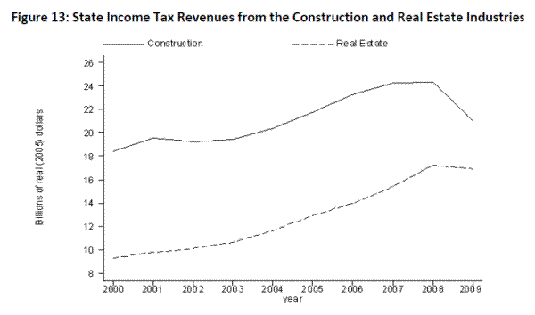
Figure 13 shows total income tax revenues attributable to labor income from the construction and real estate industries aggregated across all states. Income tax revenues from the construction industry peaked at $24 billion in 2008 and stepped down to $21 billion in 2009. This time series is largely driven by changes in employment, which fell from 11 million in 2008 to 9 million in 2009. By contrast, average tax payments per job in the construction industry continued to increase in real terms through 2009. One reason why the drop in housing-related income tax revenues was not more severe is that construction employment was supported in 2007 and 2008 by the nonresidential sector, which peaked several years after the residential sector. In addition, the drop in residential construction employment has been larger than that in the nonresidential sector. Consequently, if we were able to disaggregate the state-level data into these two components, we would likely find that the contraction in income tax revenues from residential construction began earlier and was more severe than that of the nonresidential sector.
In the smaller real estate industry, income tax revenues peaked at $17.2 billion in 2008 and edged down to $16.9 billion in 2009. The decline in employment was less pronounced in the real estate industry than in the construction industry, likely because it includes categories like lessors of real estate and property managers, which are less-closely tied to owner-occupied real estate values.
Adding the two industries together and using the peak year method, income tax revenues from housing-related industries were 9 percent ($3.3 billion) higher in 2009 than they had been in 2005 at the peak of the housing market boom. As mentioned above and illustrated in the figure, income tax revenues from these industries continued to increase even as the housing market contracted. They did not start to fall until 2009, when they dropped by 9 percent ($3.6 billion).
Turning to the trend growth simulation, we assume that real average wages and employment in each industry increased at their 1995-2002 trends and use Taxsim to calculate the implied counterfactual personal income tax revenue in 2009 attributable to each industry. The counterfactual level of collections is $46.8 billion-23 percent ($8.8 billion) higher than our estimates of actual 2009 tax revenues. Although this gap seems large, aggregate real state income tax revenues were $216 billion in 2009. Thus, aggregate income tax revenues would only have been about 4 percent higher had revenues from housing-related industries increased at trend through 2009.
V. Combining the Channels
In this section, we combine the estimated effects of each channel to obtain a total effect on all forms of revenue. Because property tax revenues appear to be unresponsive to declines in house prices (at least through the end of 2009), we focus on changes in state revenues due to the other four channels.
Table 2 reports the change in housing-related revenues from 2005 to 2009 (the peak method). Focusing first on the national estimates (final row), the transfer tax, the direct sales tax, and the indirect sales tax effects reduce total revenue by about $6 billion, $7 billion, and $5 billion, respectively. The income tax effect is a net positive in this calculation, because in most states construction employment increased from 2005 to 2009. The sum of these effects reduced state revenues by $15 billion. Columns 6 through 10 of the table compare these estimates to total 2005 tax revenues from each source. The transfer tax fell by 53 percent during this period. The large magnitude of this percentage effect is not surprising because residential housing comprises a large portion of the transfer tax base. By contrast, the other effects are more modest. The direct sales tax channel reduced sales tax revenues by 3 percent from 2005 to 2009, and the indirect sales tax effect reduced sales tax revenue by 2 percent. Adding the components together, total tax revenues (including corporate income and other taxes not included in our analysis) were reduced by 2 percent from 2005 to 2009. Although a reduction in total revenue of this magnitude is not insignificant, the decline occurred over several years which likely reduced the impact on state governments. For comparison, total revenues fell by 5 percent in 2009, likely as the result of the broader economic recession.
The table also reveals considerable heterogeneity across states. Not surprisingly, Florida, Nevada, and Arizona suffered the largest losses in percentage terms. Tax revenues in California also decreased substantially (the 2![]() largest drop in billions of dollars), but this decrease was only the 11
largest drop in billions of dollars), but this decrease was only the 11![]() largest as a percent of total tax revenues. Other states that experienced
relatively large declines are Virginia, Minnesota, and Michigan. On the other hand, a large number of states have not experienced any notable drop in tax revenue. We estimate that the housing channels either boosted total tax revenues or reduced them by less than 1 percent in 26 states.
largest as a percent of total tax revenues. Other states that experienced
relatively large declines are Virginia, Minnesota, and Michigan. On the other hand, a large number of states have not experienced any notable drop in tax revenue. We estimate that the housing channels either boosted total tax revenues or reduced them by less than 1 percent in 26 states.
Table 3 reports similar results for the "trend growth" simulation method. Total tax revenues in 2009 were $31 billion lower than predicted by trend. All four channels contribute noticeably to this deficit, although the direct sales tax and personal income tax effects are larger than the other two channels. To estimate the percentage effect of this deficit, we predict what total tax revenues would have been had the housing components expanded at trend. We find that total state tax revenues in 2009 were 5 percent lower than they would have been had the housing market continued at its 1995-2002 trend.
V. Conclusions
State and local tax revenues have suffered a sharp downturn in the past several years, at the same time as the housing market contracted appreciably. In this paper we attempt to disentangle the direct impact of the housing market downturn on state and local tax receipts from the impact of the general economic recession. We come to two primary conclusions. First, we find that property tax collections have been surprisingly resilient due to both the long lags between changes in the market value of property and changes in taxable assessments and the tendency of policy makers to insulate revenues from housing price declines by raising tax rates. This propensity makes it unlikely that property tax revenues will fall sharply in coming years. Second, although the housing market downturn has reduced states' collections of transfer taxes, sales taxes and personal income taxes, the magnitude of this effect is relatively modest, particularly when viewed against the recent plunge in aggregate tax receipts. Thus, the downturn in state and local tax revenues was likely driven by the economic recession rather than the direct influence of the housing market downturn.
References
Attanasio, Orazio, Laura Blow, Robert Hamilton, and Andrew Leicester. "Booms and Busts: Consumption, House Prices and Expectations." Economica, Vol. 76, Issue 201, (February 2009): 20-50.
Behrens, John and Jane Gravelle. "Transfer Taxes, Real Estate" in The Encyclopedia of Taxation and Tax Policy, eds. Joseph Cordes, Robert Ebel and Jane Gravelle, Urban Institute Press, 2004.
Bennett, D.L. and John Perry, "Why Your're Paying Too Much in Property Taxes", Atlanta Journal-Constitution, Metro Section, December 7, 2009.
Brunori, David. Local Tax Policy: A Federalist Perspective. Washington D.C.: Urban Institute Press, 2003.
Carlson, Mark. "Some Findings Regarding Monetary Policy and the Ending of House Price Bubbles", mimeo, Federal Reserve Board, 2010.
Case, Karl E, John M. Quigley, and Robert J. Shiller. "Comparing Wealth Effects: The Stock Market versus the Housing Market." The B.E. Journal of Macroeconomics, advances. 5, issue 1, number 1, 2005.
Cooper, Daniel. "Impending U.S. Spending Bust? The Role of Housing Wealth as Borrowing Collateral." Federal Reserve Bank of Boston Public Policy Discussion Paper Series, No. 09-9, 2009.
Dynan, Karen. "Wealth Effects and the Changing Economy," mimeo, Brookings Institution, 2010.
Dye, Richard and Andrew Reschovsky. "Property Tax Responses to State Aid Cuts in the Recent Fiscal Crisis." Public Budgeting & Finance, Vol. 28, Issue 2, (Summer, 2008): 87-111.
Giertz, J. Fred. "The Property Tax Bound." National Tax Journal 59 No. 3 (September, 2006): 695-705.
Lutz, Byron. "The Connection Between House Price Appreciation and Property Tax Revenues", National Tax Journal, Vol. LXI, No. 3, September 2008.
Mian, Atif R. and Amir Sufi. "House Prices, Home Equity-Based Borrowing, and the U.S. Household Leverage Crisis." Chicago Booth Research Paper No. 09-20, 2009.
Wiseman, Paul, "Homeowners Balk as Property Tax Bills Stay High", USA Today, Money Section, March 20, 2010.
| (1) |
(2) |
(3) |
(4) |
|
| 0.86
(0.10) |
||||
| 0.71
(0.09) |
0.62
(0.09) |
0.58
(0.64) |
||
| 1.59
(0.19) |
1.49
(0.11) |
1.44
(0.11) |
||
| Exclude States with "Progressive" Tax Structures | X | X | ||
| Exclude States with a Tax Rate Increase Between 1999 and 2009 | X | |||
| Number of Observations | 307 | 307 | 228 | 168 |
| State | (1) transfer ($millions) | (2) direct sales ($millions) | (3) indirect sales ($millions) | (4) income ($millions) | (5) total ($millions) | (6) transfer (%) | (7) direct sales (%) | (8) indirect sales (%) | (9) income (%) | (10) total (%) |
| AL | -13 | -46 | -1 | 63 | 3 | -26 | -2 | 0 | 2 | 0 |
| AK | 0 | 0 | 0 | 0 | 0 | . | . | . | . | 0 |
| AZ | 0 | -471 | -130 | -63 | -664 | . | -9 | -3 | -2 | -6 |
| AR | -7 | -47 | -5 | 62 | 2 | -17 | -2 | 0 | 3 | 0 |
| CA | 0 | -1,016 | -1,905 | 772 | -2,150 | . | -3 | -6 | 2 | -2 |
| CO | 0 | -106 | -31 | -20 | -156 | . | -5 | -1 | -1 | -2 |
| CT | -110 | -41 | -78 | -11 | -240 | -51 | -1 | -2 | 0 | -2 |
| DE | -44 | 0 | 0 | 11 | -33 | -32 | . | . | 1 | -1 |
| DC | -114 | -5 | -6 | -19 | -144 | -32 | -1 | -1 | -1 | -3 |
| FL | -3,564 | -1,476 | -535 | 0 | -5,575 | -72 | -7 | -3 | . | -14 |
| GA | 0 | -369 | -69 | 168 | -270 | . | -7 | -1 | 2 | -2 |
| HI | -15 | -25 | 3 | 33 | -3 | -37 | -1 | 0 | 2 | 0 |
| ID | 0 | -96 | -8 | 35 | -69 | . | -9 | -1 | 3 | -2 |
| IL | -57 | -329 | -210 | 145 | -450 | -50 | -4 | -3 | 2 | -2 |
| IN | 0 | -108 | -65 | 50 | -123 | . | -2 | -1 | 1 | -1 |
| IA | -3 | -13 | -9 | 71 | 46 | -19 | -1 | -1 | 3 | 1 |
| KS | 0 | -24 | -14 | 109 | 72 | . | -1 | -1 | 5 | 1 |
| KY | -1 | -67 | -19 | 80 | -6 | -24 | -2 | -1 | 3 | 0 |
| LA | 0 | -16 | 3 | 280 | 268 | . | -1 | 0 | 13 | 3 |
| ME | -10 | -24 | -7 | 12 | -29 | -27 | -2 | -1 | 1 | -1 |
| MD | -136 | -53 | -86 | 15 | -260 | -51 | -2 | -3 | 0 | -2 |
| MA | -141 | -63 | -182 | 117 | -268 | -53 | -2 | -5 | 1 | -1 |
| MI | -212 | -238 | -334 | -55 | -839 | -67 | -3 | -4 | -1 | -3 |
| MN | -150 | -158 | -127 | -166 | -601 | -47 | -4 | -3 | -3 | -4 |
| MS | 0 | -22 | -11 | 83 | 51 | . | -1 | 0 | 7 | 1 |
| MO | -4 | -82 | -47 | 111 | -22 | -32 | -3 | -2 | 3 | 0 |
| MT | 0 | 0 | 0 | 10 | 10 | . | . | . | 1 | 1 |
| NE | -2 | -11 | -8 | 3 | -18 | -19 | -1 | -1 | 0 | 0 |
| NV | -105 | -264 | -119 | 0 | -487 | -61 | -9 | -4 | . | -8 |
| NH | -66 | 0 | 0 | 0 | -66 | -39 | . | . | 0 | -3 |
| NJ | -281 | -101 | -191 | 169 | -404 | -47 | -2 | -3 | 2 | -2 |
| NM | 0 | -41 | 0 | 39 | -1 | . | -3 | 0 | 5 | 0 |
| NY | -349 | -126 | -76 | 866 | 315 | -29 | -1 | -1 | 3 | 1 |
| NC | -15 | -224 | 0 | 150 | -89 | -22 | -5 | 0 | 2 | 0 |
| ND | 0 | 5 | 1 | 13 | 19 | . | 1 | 0 | 5 | 1 |
| OH | 0 | -191 | -143 | -159 | -493 | . | -2 | -2 | -2 | -2 |
| OK | -1 | -25 | 0 | 19 | -8 | -9 | -1 | 0 | 1 | 0 |
| OR | -3 | 0 | 0 | 48 | 45 | -33 | . | . | 1 | 1 |
| PA | -149 | -113 | -17 | 48 | -231 | -25 | -1 | 0 | 1 | -1 |
| RI | -9 | -10 | -42 | -7 | -68 | -62 | -1 | -5 | -1 | -3 |
| SC | -27 | -138 | -17 | 60 | -122 | -33 | -5 | -1 | 2 | -2 |
| SD | 0 | 0 | 0 | 0 | -1 | 0 | 0 | 0 | . | 0 |
| TN | -54 | -192 | -12 | 0 | -258 | -26 | -3 | 0 | 0 | -2 |
| TX | 0 | -541 | -81 | 0 | -622 | . | -3 | 0 | . | -2 |
| UT | 0 | -72 | 7 | 138 | 74 | . | -4 | 0 | 7 | 1 |
| VT | -7 | -6 | -4 | 2 | -14 | -31 | -2 | -1 | 0 | -1 |
| VA | -405 | -120 | -138 | -118 | -780 | -58 | -4 | -4 | -1 | -5 |
| WA | -328 | -197 | 26 | 0 | -499 | -34 | -2 | 0 | . | -3 |
| WV | -6 | -18 | -21 | 75 | 29 | -48 | -2 | -2 | 6 | 1 |
| WI | -30 | -97 | -44 | 6 | -165 | -37 | -2 | -1 | 0 | -1 |
| WY | 0 | -2 | -1 | 0 | -3 | . | 0 | 0 | . | 0 |
| TOTAL | -6,416 | -7,375 | -4,753 | 3,246 | -15,297 | -53 | -3 | -2 | 1 | -2 |
| State | (1) transfer, 2009 housing - predicted 2009 housing ($millions) |
(2) direct sales, 2009 housing - predicted 2009 housing ($millions) |
(3) indirect sales, 2009 housing - predicted 2009 housing ($millions) |
(4) income, 2009 housing - predicted 2009 housing ($millions) |
(5) total, 2009 housing - predicted 2009 housing ($millions) |
(6) transfer, (2009 housing - predicted 2009 housing)/ (2009 total) (%) |
(7) direct sales, (2009 housing - predicted 2009 housing)/ (2009 total) (%) |
(8) indirect sales, (2009 housing - predicted 2009 housing)/ (2009 total) (%) |
(9) income, (2009 housing - predicted 2009 housing)/ (2009 total) (%) |
(10) total, (2009 housing - predicted 2009 housing)/ (2009 total) (%) |
| AL | -13 | -14 | -13 | 8 | -32 | -38 | -1 | -1 | 0 | 0 |
| AK | 0 | 0 | 0 | 0 | 0 | . | . | . | . | 0 |
| AZ | 0 | -517 | -92 | -142 | -751 | . | -11 | -2 | -7 | -8 |
| AR | -7 | -29 | -13 | -20 | -69 | -32 | -1 | -1 | -1 | -1 |
| CA | 0 | -2060 | -1,923 | -955 | -4,938 | . | -7 | -7 | -2 | -5 |
| CO | 0 | -184 | -125 | -645 | -954 | . | -10 | -7 | -17 | -13 |
| CT | -75 | -48 | -107 | -310 | -540 | -97 | -2 | -4 | -5 | -5 |
| DE | 2 | 0 | 0 | -27 | -25 | 3 | . | . | -3 | -1 |
| DC | -284 | -5 | -14 | -44 | -347 | -187 | -1 | -2 | -4 | -8 |
| FL | -1,800 | -1573 | -358 | 0 | -3,731 | -161 | -10 | -2 | . | -13 |
| GA | 0 | -559 | -155 | -263 | -977 | . | -10 | -3 | -4 | -7 |
| HI | 2 | -16 | 49 | 164 | 200 | 7 | -1 | 2 | 14 | 5 |
| ID | 0 | -88 | 1 | 27 | -60 | . | -9 | 0 | 3 | -2 |
| IL | -49 | -498 | -353 | -329 | -1,229 | -158 | -8 | -6 | -4 | -5 |
| IN | 0 | -246 | -92 | -86 | -424 | . | -5 | -2 | -2 | -3 |
| IA | -4 | -66 | -22 | 0 | -93 | -41 | -4 | -1 | 0 | -2 |
| KS | 0 | -38 | -30 | -1 | -69 | . | -2 | -1 | 0 | -1 |
| KY | -1 | -106 | -40 | -77 | -224 | -51 | -4 | -2 | -3 | -3 |
| LA | 0 | -33 | -21 | 118 | 63 | . | -1 | -1 | 4 | 1 |
| ME | -16 | -58 | -16 | -81 | -171 | -99 | -7 | -2 | -7 | -6 |
| MD | -63 | -134 | 2 | -173 | -368 | -61 | -4 | 0 | -3 | -3 |
| MA | -239 | -50 | -412 | -741 | -1,442 | -193 | -1 | -11 | -8 | -8 |
| MI | -394 | -348 | -591 | -820 | -2,153 | -343 | -4 | -7 | -15 | -10 |
| MN | -358 | -392 | -281 | -774 | -1,805 | -235 | -10 | -7 | -13 | -12 |
| MS | 0 | -35 | -3 | -2 | -40 | . | -1 | 0 | 0 | -1 |
| MO | -6 | -113 | -81 | -151 | -351 | -76 | -4 | -3 | -4 | -4 |
| MT | 0 | 0 | 0 | 2 | 2 | . | . | . | 0 | 0 |
| NE | -4 | -33 | -21 | -63 | -120 | -39 | -3 | -2 | -4 | -3 |
| NV | -3 | -285 | -51 | 0 | -339 | -5 | -12 | -2 | . | -6 |
| NH | -112 | 0 | 0 | 0 | -112 | -158 | . | . | 0 | -6 |
| NJ | -94 | -261 | -232 | -541 | -1,128 | -36 | -4 | -3 | -6 | -5 |
| NM | 0 | -54 | 14 | 33 | -8 | . | -3 | 1 | 5 | 0 |
| NY | -323 | -301 | -190 | -949 | -1,763 | -62 | -3 | -2 | -3 | -3 |
| NC | -19 | -326 | -44 | -296 | -685 | -66 | -7 | -1 | -3 | -4 |
| ND | 0 | 5 | -4 | 9 | 10 | . | 1 | -1 | 3 | 1 |
| OH | 0 | -308 | -229 | -385 | -921 | . | -5 | -3 | -5 | -4 |
| OK | -4 | -38 | -16 | 31 | -27 | -36 | -2 | -1 | 1 | 0 |
| OR | -1 | 0 | 0 | -168 | -169 | -14 | . | . | -4 | -3 |
| PA | -12 | -275 | 24 | -251 | -514 | -4 | -4 | 0 | -3 | -2 |
| RI | -5 | -21 | -38 | -110 | -174 | -82 | -3 | -5 | -13 | -7 |
| SC | -26 | -217 | -56 | -75 | -374 | -120 | -9 | -2 | -4 | -6 |
| SD | 0 | -13 | -3 | 0 | -17 | -31 | -2 | -1 | . | -1 |
| TN | -87 | -137 | -72 | 0 | -296 | -74 | -2 | -1 | 0 | -3 |
| TX | 0 | -1165 | -315 | 0 | -1,480 | . | -6 | -2 | . | -4 |
| UT | 0 | -45 | 4 | 77 | 36 | . | -3 | 0 | 4 | 1 |
| VT | -5 | -20 | -7 | -10 | -41 | -71 | -7 | -2 | -2 | -2 |
| VA | -162 | -248 | -84 | -483 | -977 | -57 | -8 | -3 | -6 | -7 |
| WA | -321 | -182 | -26 | 0 | -529 | -94 | -2 | 0 | . | -4 |
| WV | -2 | -33 | -12 | 57 | 10 | -25 | -3 | -1 | 4 | 0 |
| WI | -40 | -192 | -88 | -376 | -696 | -128 | -5 | -2 | -7 | -5 |
| WY | 0 | 1 | -2 | 0 | 0 | . | 0 | 0 | . | 0 |
| TOTAL | -4,525 | -11,359 | -6,137 | -8,822 | -30,844 | -110 | -6 | -3 | -4 | -5 |
