Skip to: [Printable Version (PDF)] [Bibliography] [Footnotes]

Finance and Economics Discussion Series: 2011-19 Screen Reader version ^♣

Dynamic Factor Value-at-Risk for Large,
Heteroskedastic Portfolios*

Sirio Aramonte

Federal Reserve Board

Marius del Giudice Rodriguez

Federal Reserve Board

Jason J. Wu**

Federal Reserve Board

Keywords: Value-at-Risk, dynamic factor models, stock portfolios

Abstract:

Trading portfolios at financial institutions are typically driven by a large number of financial variables. These variables are often correlated with each other and exhibit by time-varying volatilities. We propose a computationally efficient Value-at-Risk (VaR) methodology based on Dynamic Factor Models (DFM) that can be applied to portfolios with time-varying weights, and that, unlike the popular Historical Simulation (HS) and Filtered Historical Simulation (FHS) methodologies, can handle time-varying volatilities and correlations for a large set of financial variables. We test the DFM-VaR on three stock portfolios that cover the 2007-2009 financial crisis, and find that it reduces the number and average size of back-testing breaches relative to HS-VaR and FHS-VaR. DFM-VaR also outperforms HS-VaR when applied risk measurement of individual stocks that are exposed to systematic risk.

JEL Classification: C1, C22, C22.

1 Introduction

As described in Berkowitz & O'Brien (2002) and Berkowitz & O'Brien (2006), trading portfolios at large financial institutions exhibit two key characteristics: they are driven by a large number of financial variables, such as stock returns, credit spreads, or yield curves, and these variable have time-varying volatilities and correlations. To accurately capture risks in such portfolios, it is important for risk managers to select Value-at-Risk (VaR) methodologies that adequately handle these two characteristics. This paper presents one such VaR methodology that is based on Dynamic Factor Models (DFM, see for instance Stock & Watson (2002)).

When a trading portfolio is driven by a large number of financial variables, Historical Simulation (HS-VaR) is the standard industry practice for computing VaR measures (see, among others, Perignon & Smith (2010) and Berkowitz et al. (2009)). HS-VaR treats past realizations of the financial variables as scenarios for future realizations. Although the HS-VaR is easy to compute, it is not well-suited to capture the time-varying volatilities in financial variables (Pritsker (2006)). Barone-Adesi et al. (1999) and Hull & White (1998) introduced Filtered Historical Simulation (FHS-VaR) as a way of handling time-varying volatility in VaR estimation. In cases where the VaR depends on multiple financial variables, Barone-Adesi et al. (1999) and Pritsker (2006) suggest filtering each variable independently. Univariate filtering imposes a high computational burden, because filtering must be done one variable at a time.¹ In addition, FHS-VaR does not explicitly capture time-varying correlations among the financial variables, which may be important particularly during times of financial stress.

We introduce DFM-VaR as a means of capturing the time-varying volatilities and correlations of a large number of financial variables in a VaR estimation. Our main assumption is that the large panel of variables are driven by a smaller set of latent factors. By modeling financial variables through a DFM with time-varying volatilities and correlations among the latent factors, the number of volatilities and correlations to be estimated is greatly reduced, resulting in computational efficiency.

To evaluate whether the DFM-VaR accurately captures risks in financial markets, we combine the DFM with the Dynamic Conditional Correlation (DCC) model of Engle (2002) to estimate VaRs for three stock portfolios: one equally-weighted portfolio of large US stocks, one portfolio with time-varying weights based on momentum, and one portfolio with time-varying weights based on the slope of option implied volatility smile. Several DFM-VaRs with different specifications are compared to the HS-VaR and the FHS-VaR based on univariate filtering. We find that the DFM-VaRs perform better than HS-VaR and FHS-VaR in terms of back-testing breaches and average breach-size in most cases. As expected, the DFM-VaRs were much more efficient to estimate than the FHS-VaR.

We would like to emphasize that our innovation is to use DFM as a way to model VaR in an environment where a large panel of financial variables exhibit time-varying volatilities. The general idea of combining latent factors with GARCH was proposed by Alexander (2001) and Alexander (2002), while theoretical properties of DFM-DCC models were explored by Alessi et al. (2009). These studies provide a platform for this paper to demonstrate how the DFM can be applied effectively in portfolio risk management.

The remainder of the paper is organized as follows. Section 2 describes the general framework for VaR estimation. Section 3 further describes the HS-VaR and FHS-VaR approaches to which we compare the DFM-VaR methodology. Section 4 details the estimation of the DFM-VaR. Section 5 introduces the data and the three test portfolios we use in the empirical analysis. Performances of the VaRs and the associated statistical tests are documented in Section 6. In Section 7, we provide robustness tests to show how the DFM-VaR measures risk for individual stocks which are sensitive to systematic shocks. The last section contains concluding remarks and thoughts for future research. Tables and figures can be found in the Appendix.

2 Economic Problem

Focusing on a one period holding horizon for a trading portfolio,² the objective is to calculate the VaR of a portfolio of traded assets, conditional on the information available at time .³

Let $P\&L_{T+1}$ be the profit-and-loss of the portfolio at , and $\mathcal{I}_{T}$ the information set up to time . The definition of VaR at level $\alpha\in (0,1)$ is:

$\displaystyle VaR_{T+1}^{\alpha}=sup\{l\in\mathcal{R}:P(P\&L_{T+1}<l\vert\mathcal{I}_{T})\le 1-\alpha\}$

(2.1)

Assume that $P\&L_{t}$ can be calculated as:

$\displaystyle P\&L_{t}=g(\mathbf{X}_{t},\theta_{t})$

(2.2)

where $\mathbf{X}_{t}$ is a $N\times 1$ vector of financial variables, where

is large, and $\theta_{t}$ is a vector of possibly time-varying parameters, like portfolio weights or parameters from pricing models. For example, the profit-and-loss at time

of the S&P 500 can be represented as:

$\displaystyle g(\mathbf{X}_{t},\theta_{t})=\theta^{'}_{t}\mathbf{X}_{t}$

(2.3)

where $\mathbf{X}_{t}$ is a $500\times 1$ vector of returns of each S&P component, $\theta_{t}$ is a $500\times 1$ vector with each element equal to 0.2%, and the initial investment was assume to be 1.

When using (2.2) to calculate VaR conditional on $\mathcal{I}_{T}$ , we assume that $\theta_{T+1}$ is known at .⁴ The goal is to estimate the conditional distribution of $P\&L_{T+1}\vert\mathcal{I}_{T}$ and choose its $(1-\alpha)^{th}$ quantile as the VaR estimate, as in (2.1). Under the assumption that $\theta_{T+1}$ is known, the problem reduces to the estimation of the conditional distribution $\mathbf{X}_{T+1}\vert\mathcal{I}_{T}$ . For this purpose, the risk manager can obtain either parametric or nonparametric estimates of the distribution of $\mathbf{X}_{T+1}$ . He then either obtains a closed form solution for the conditional distribution of $P\&L_{T+1}$ , or makes draws to obtain scenarios for that distribution. The latter case is usually referred to as the simulation approach to VaR.

3 Historical and Filtered Historical Simulation

Deriving the distribution of $\mathbf{X}_{T+1}$ becomes difficult when its dimension is large. In such cases, the standard practice is to use HS-VaR, where past realizations of $\mathbf{X}_{t}$ are used to build the distribution of $\mathbf{X}_{T+1}$ . The only choice the risk manager faces is the length of the data window. For instance, it is popoular in the industry to use realizations of $\mathbf{X}_{t+1}$ in the past 250 trading days as the empirical distribution of $\mathbf{X}_{T+1}$ .

Given that HS-VaR is not well suited to handling time-varying volatilities in $\mathbf{X}_{t}$ (Pritsker (2006)), researchers have embraced FHS-VaR. FHS-VaR first "filters" each variable in $\mathbf{X}_{t}$ using an appropriate volatility model (typically GARCH), then uses the estimated volatility models to forecast the volatilities of the variables at , and finally assigns the volatility forecasts to scenarios of filtered variables (i.e., variables divided by the estimated volatilities) to generate scenarios for $\mathbf{X}_{T+1}$ .⁵

Implementation of FHS-VaR runs into two issues when is large. First, because each variable in $\mathbf{X}_{t}$ is modeled individually, FHS-VaR does not capture correlations between time-varying volatilities - only unconditional correlations among the filtered variables are captured (Pritsker (2006)). Second, estimating a separate time-varying volatility model for each variable typically requires a significant computational effort.

An obvious alternative to univariate filtering is to construct FHS-VaR using multivariate time-varying volatility models, as in Engle & Kroner (1995) or Engle (2002). These methods have the potential to capture correlations, but do not lighten the computational burden, because the number of parameters to be estimated is typically in proportion to . Recent papers such as Engle & Kelly (2009), Engle (2007) and Engle et al. (2007) have proposed solutions to modeling multivariate time-varying volatilities based on various dimension reduction techniques. The DFM-VaR that we introduce also operates by reducing the dimensionality of the problem. The appealing feature of the DFM framework is that it relates closely to the factor model analysis of asset returns (e.g., Fama & French (1996)).

4 DFM-VaR Methodology

The applications and properties of DFMs have been documented by, among others, Stock & Watson (2002), Bai & Ng (2007), Bai (2003), and Bai & Ng (2006). Our proposal is to model $\mathbf{X}_{t}$ as a DFM with time-varying volatility. Various implementations of this type of model have been discussed by Alexander (2001), Alexander (2002) and Alessi et al. (2009). The model we adopt for VaR estimation follows closely to that of Alessi et al. (2009). In particular, we use the DCC volatility model of Engle (2002). While possible alternative specifications include square root processes (Cox et al. (1985)), or jumps in addition to stochastic volatility, we focus on the set of GARCH models because the theoretical properties of the DFM-GARCH has already been analyzed by Alessi et al. (2009).

Let the financial variables $\mathbf{X}_{t}$ be a vector stationary process with mean zero. The DFM model posits that $\mathbf{X}_{t}$ can be decomposed into a systematic component, driven by a $k\times 1$ vector of latent factors $f_{t}$ , and an idiosyncratic component $\varepsilon_{t}$ . The key is that , so that the variation of a large number of variables can be explained with a small set of systematic factors:

$\displaystyle \mathbf{X}_{t}$	$\displaystyle =$	$\displaystyle \lambda(L)f_{t}+\varepsilon_{t}$	(4.1)
$\displaystyle \Phi(L)f_{t}$	$\displaystyle =$	$\displaystyle hu_{t}$	(4.2)

where $\lambda(L)$ is an $N\times k$ lag polynomial of order $p_{X}$ (the factor loadings), and $\Phi(L)$ is a $k\times k$ lag polynomial of order $p_{f}$ . Notice that (4.2) states that the factors $f_{t}$ have a $p_{f}$ order Vector Auto-Regressive (VAR) representation, with a $k\times 1$ vector of common shocks $u_{t}$ . Time-varying volatilities in $\mathbf{X}_{t}$ is modeled via time-varying volatilities in the common shocks process $u_{t}$ , such that

$\displaystyle u_{t}$

$\displaystyle =$

$\displaystyle Q_{t}^{1/2}z_{t}$

(4.3)

Following Engle (2002) and Engle & Sheppard (2008), $Q_{t}$ is modeled with a DCC specification:

$\displaystyle Q_{t}$	$\displaystyle =$	$\displaystyle D_{t}W_{t}D_{t}$
$\displaystyle D_{t}$	$\displaystyle =$	diagonal matrix with $q_{it}$ on the diagonals, for
$\displaystyle q_{it}$	$\displaystyle =$	$\displaystyle \omega_{i}+\sum_{j=1}^{m_{i}}\alpha_{ij}u_{i,t-j}^{2}+\sum_{j=1}^{n_{i}}\beta_{ij}q_{i,t-j}$
$\displaystyle W_{t}$	$\displaystyle =$	$\displaystyle C^{-1}_{t}C_{t}C^{-1}_{t}$	(4.4)
$\displaystyle C_{t}$	$\displaystyle =$	$\displaystyle (1-\sum_{j=1}^{m}\alpha_{j}^{c}-\sum_{j=1}^{n}\beta_{j}^{c})\bar{C}+\sum_{j=1}^{m}\alpha_{j}^{c}(\tilde{u}_{t-j}\tilde{u}^{'}_{t-j})+\sum_{j=1}^{n}\beta_{j}^{c}C_{t-j}$
$\displaystyle C^{*}$	$\displaystyle =$	$\displaystyle diag(C_{t})^{1/2}$
$\displaystyle \tilde{u}_{t}$	$\displaystyle =$	$\displaystyle D_{t}^{-1}u_{t}\nonumber$

and $\bar{C}$ is the unconditional covariance of $\tilde{u}_{t}$ . In this model, correlations between the volatilities of the elements in $\mathbf{X}_{t}$ are captured by the dynamic factors.

In addition, to facilitate the computation of VaR, we impose that the error vector $(z_{t}^{'},\varepsilon_{t}^{'})'$ is IID across time. This assumption does not rule out contemporaneous cross-sectional correlation between elements of the error vector.

If $p_{X}=p_{f}\equiv p$ , we can re-write the above model in a State Space (SS) representation with a single lag,⁶

$\displaystyle \mathbf{X}_{t}$	$\displaystyle =$	$\displaystyle \Lambda F_{t}+\varepsilon_{t}$	(4.5)
$\displaystyle F_{t}$	$\displaystyle =$	$\displaystyle A F_{t-1}+Hu_{t}$	(4.6)

where $F_{t}=(f_{t}^{'},...,f_{t-p}^{'})'$ is an $r\equiv(p+1)\times k$ vector of static factors, $\Lambda$ is a $N\times r$ loadings matrix whose elements are a function of the loading coefficients in $\lambda(L)$ and of the coefficients in lag polynomial $\Phi(L)$ , and

is a matrix of zeros except the first $k\times k$ block, which is

Let $\mathcal{I}_{T}$ be information up to and including time . Then, to obtain the forecast distribution of $\mathbf{X}_{T+1}$ conditional on $\mathcal{I}_{T}$ , we can use the SS representation as follows:

$\displaystyle \mathbf{X}_{T+1}$	$\displaystyle =$	$\displaystyle \Lambda F_{T+1}+\varepsilon_{T+1}$
$\displaystyle F_{T+1}$	$\displaystyle =$	$\displaystyle AF_{T}+HQ^{1/2}_{T+1}z_{T+1}.$

Note, to get a forecast distribution of $\mathbf{X}_{T+1}$ , we need forecasts of the conditional variance $Q_{T+1}$ given $\mathcal{I}_{T}$ , and of the conditional distribution of $(z_{T+1}^{'},\varepsilon_{T+1}^{'})'$ given $\mathcal{I}_{T}$ . But since $(z_{t}^{'},\varepsilon_{t}^{'})'$ are assumed to be IID across

, the conditional distribution is the same as the unconditional distribution. In finite samples, one can use the observed data $\{\mathbf{X}_{t}\}_{t=1}^{T}$ to estimate the factors $\widehat{F}_{1},...,\widehat{F}_{T}$ , the various coefficient matrices, and the shocks process $\{(z_{t}^{'},\varepsilon_{t}^{'})^{'}\}_{t=1}^{T}$ . Assuming that

and

are known⁷, VaR estimation based on DFM-DCC can be implemented with the following steps:

Step 1.

Using the Principal Components (PC) methods of Stock & Watson (2002), Bai (2003) and Bai & Ng (2006), obtain the following estimates for $\Lambda$ , $\{F_{t}\}_{t=1}^{T}$ , and $\{\varepsilon_{t}\}_{t=1}^{T}$ :

$\displaystyle \widehat{\Lambda}$	$\displaystyle =$	eigen-vectors of $\frac{1}{T}\sum_{t=1}^{T}\mathbf{X}_{t}\mathbf{X}_{t}'$ corresponding to the largest eigenvalues
$\displaystyle \widehat{F}_{t}$	$\displaystyle =$	$\displaystyle \widehat{\Lambda}^{'}\mathbf{X}_{t}$ , for
$\displaystyle \widehat{\varepsilon}_{t+1}$	$\displaystyle =$	$\displaystyle \mathbf{X}_{t}-\widehat{\Lambda}\widehat{F}_{t}$

Step 2.

With the estimated static factors $\{\widehat{F}_{t}\}_{t=1}^{T}$ , run the vector autoregression in (4.6), obtain coefficient estimates $\widehat{A}$ , and VAR residuals $\widehat{Hu_{t}}$ . Following Alessi et al. (2009), estimate

using

$\displaystyle \widehat{H}=$ first

eigen-vectors of $\displaystyle \frac{1}{T}\sum_{t=1}^{T}\widehat{Hu_{t}}\widehat{Hu_{t}}^{'}$

Then, estimate $u_{t}$ by $\widehat{u}_{t}=\widehat{H}^{'}\widehat{Hu_{t}}$ .

Step 3.

Use $\{\widehat{u}_{t}\}_{t=1}^{T}$ to estimate the DCC model in (4.5), obtain estimates of the DCC parameters, $\{\widehat{Q}_{t}\}_{t=1}^{T}$ and $\{\widehat{z}_{t}\}_{t=1}^{T}$ . Using these, build the $k\times k$ conditional variance-covariance matrix forecast $\widehat{Q}_{T+1}$ .⁸

Step 4.

Finally, build scenarios for $\mathbf{X}_{T+1}$ using $\mathbf{X}^{*}_{T+1}=\widehat{\Lambda}(\widehat{A}\widehat{F}_{T}+\widehat{H}\widehat{Q}_{T+1}^{1/2}z^{*}_{T+1})+\varepsilon^{*}_{T+1}$ , where $(z_{T+1}^{*'},\varepsilon_{T+1}^{*'})^{'}$ are drawn from $(\widehat{z}_{1}^{'},\widehat{\varepsilon}_{1}^{'})',....,(\widehat{z}_{T}^{'},\widehat{\varepsilon}_{T}^{'})'$ . One can then build scenarios for $P\&L_{T+1}$ as $P\&L^{*}_{T+1}=g(\mathbf{X}_{T+1}^{*},\theta_{T+1})$ , and choose the appropriate percentile as the VaR estimate ${VaR}^{\alpha}_{T+1}$ .

Drawing an arbitrarily large number of times from the

scenarios will yield the same results as using each of the

scenarios once. Therefore, there is no need to use each of the

scenarios more than once. In other words, ${VaR}_{T+1}^{\alpha }$ will be the appropriate quantile chosen out of the

ordered $P\&L^{*}_{T+1}$ scenarios.

Finally, using PCs to estimate DFMs will yield factors and loadings that are identified up to a unitary transformation. However, the common component $\Lambda F$ and the idiosyncratic shocks $\varepsilon$ are exactly identified. It follows from the results of Alessi et al. (2009) that, if one imposes the additional restriction that $\vert\vert\widehat{u}_{t}-u_{t}\vert\vert=o_{p}(1)$ , the scenarios of $\mathbf{X}^{*}_{T+1}$ form a distribution that consistently estimates the true conditional distribution of $\mathbf{X}_{T+1}\vert\mathcal{I}_{T}$ as $T\rightarrow\infty$ .

5 Data and Portfolio Construction

We collect daily returns on the stocks in CRSP (share codes 10 and 11) that commonly trade on the NYSE, AMEX, and NASDAQ. We use only stocks that have non-missing returns on almost all trading days from 2007 to 2009. Our final data set contains daily returns on 3,376 stocks across 750 trading days. All VaRs (DFM-VaR, HS-VaR and FHS-VaR) are estimated using this data set, after returns of each stock are winsorized at the 0.25% and 99.75% quantiles of the returns time series distribution.

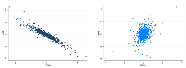
To get a flavor of the nature of the factors used to construct DFM-VaR extracted from this panel of stock returns, Table 8.1 in the Appendix reports the correlations between the first two principal components of $\frac{1}{T}\sum_{t=1}^{T}\mathbf{X}_{t}\mathbf{X}_{t}^{'}$ , $f_{1t}$ and $f_{2t}$ , and a set of asset pricing factors that includes the Fama-French and momentum factors, as well as the changes on the CBOE's VIX index and returns on the CBOE's PUT index. The VIX and the PUT indices are created to track volatility and downside risk, respectively. The results show a -95.5% correlation between $f_{1t}$ and the market, and a moderate correlation between $f_{2t}$ and both smb (35.4%) and hml (21.5%) (see Figure 8.2 in the appendix).

The high correlation between $f_{1t}$ and the market is to be expected, because much of the common variation in the returns of a large set of stocks is by definition captured by the returns on a broad equity index. The negative, rather than positive, sign is potentially due to the fact that the common factors are identified up to a unitary transformation. $f_{1t}$ is also highly correlated with several other factors, like dPut and dVix, a fact driven by the well-established correlation of the market with the same factors. The moderate but significant correlations of $f_{2t}$ with smb and hml follows from the relevance of the two factors in explaining the cross-section of stock returns (as in Fama & French (1996)). Table 8.2 reports the correlations at the height of the 2008 financial crisis (9/2008-12/2008), and it suggests that $f_{2t}$ can also capture downside and volatility risk: the correlation between $f_{2t}$ and dPut increased in magnitude to -34.4% (from -14.8% over the whole sample). The correlation with dVix also increased, from 16.3% to 35.6%. These correlation numbers are not surprising if one inspects Figure 8.1, which shows that $f_{2t}$ generally has little variation, with the exception of a cluster of large volatility and of several spikes in late 2008.

We form three test portfolios with the stock returns data: one that replicates a broad market index, one based on the momentum effect, and one that includes stocks more likely to experience large swings in prices, as proxied by the slope of the option implied volatility smile.

The first portfolio (S&P 500) is the equally-weighted average return on the S&P 500 constituents as of the end of June 2008, with weights that remain constant throughout the sample period. The second portfolio (Momentum) is the 6-6 overlapping momentum portfolio of Jegadeesh & Titman (1993). The portfolio is designed to go long/short in the stocks with the highest/lowest returns over the past six months, and is rebalanced every six months. The overlapping feature of the portfolio means that weights typically change every month. The third portfolio (Money) is based on the slope of the implied volatility smile of equity options.⁹ We define the Money portfolio as the equally-weighted average return of the stocks with the lowest regression slope coefficients (bottom 30% of the distribution in ), where the slopes are estimated in a manner similar to Bakshi et al. (2003) by regressing the log-implied volatility on the log-moneyness ( $\frac{K}{S}$ ). We focus on daily regressions, consider both in-the-money and out-of-the-money prices, and require a minimum of three observations with maturity between 20 and 40 calendar days. While our approach is more prone to picking noise in the variation of implied volatility slopes, it does provide portfolio weights that change at a higher frequency.¹⁰

Table 8.3 in the appendix presents summary statistics for the observed returns of the three portfolios. We point out that the S&P 500 portfolio has the highest mean return while the Money portfolio shows the highest volatility. We also note that the Momentum portfolio has a large negative skew, consistent with a financial crisis period.

6 VaR Estimations and Results

We compare the DFM-VaR, HS-VaR and FHS-VaR along three dimensions: the number of VaR breaches, the average size of the breaches, and computational time. The number of breaches is the primary indicator of VaR performance used in the literature as well as in bank regulation.¹¹ If the VaR model is good, we would expect that the 99% VaR, for instance, to be breached by realized portfolio 1% of the time. Average breach size is an indicator of how severe the breaches are, and a decent VaR model is expected to experience reasonablely-sized breaches. Finally, computation time of each VaR measures how efficiently the VaRs can be calculated, which is a very important practical consideration for large financial institutions.

In order to statistically assess the performance of the VaRs, numerous tests have been proposed by the literature, such as the ones in Kupiec (1995), Christoffersen & Pelletier (2004), Engle & Manganelli (2004) and Gaglianone et al. (2011). The majority of these tests are based on statistical properties of the frequency at which breaches occur. As we will describe in details, we perform two tests that are popular in the literature for all VaRs that we calculate. While an evaluation of performances of these tests are out of the scope of this paper, we remind the reader to interpret the results of these tests with caution, particularly because two of our three test portfolios changes over time.¹²

Formally, a "breach" variable can be defined as:

$\displaystyle B_{t}^{\alpha} =\left\{ \begin{array}[c]{cc} 1 & \text{if } P\&L_{t} <VaR_{t}^{\alpha}\\ 0 & \text{if } P\&L_{t} \geqslant VaR_{t}^{\alpha}\\ \end{array} \right.$

(6.1)

Therefore breaches form a sequence of zeros and ones. If the VaR model is correctly specified, the conditional probability of a VaR breach would be

$\displaystyle P(B_{t}^{\alpha}=1\vert\mathcal{I}_{t-1})= 1-\alpha\$

(6.2)

for every

. The first statistical test we use is a conditional coverage test, which is based on the that if the VaR model is correctly specified, no information available to the risk manager at the time the VaR is calculated should be helpful in forecasting the probability that the VaR will be breached.¹³ Among the set of tests belonging to this class is the one proposed in Engle & Manganelli (2004) and is usually referred to as the CaViaR (Conditional Autoregressive Value-At-Risk) test. As presented in Berkowitz et al. (2009), the test is based on the following regression

$\displaystyle B_{t}^{\alpha}=\theta+\sum_{j=1}^{n}\beta_{1j}B_{t-j}^{\alpha}+\sum_{j=1}^{n}\beta_{2j}g(B_{t-j}^{\alpha},B_{t-j-1}^{\alpha},...,P\&L_{t-j},P\&L_{t-j-1},...)+v_{t}$

(6.3)

and we set $g(B_{t-k}^{\alpha},B_{t-j-1}^{\alpha},...,P\&L_{t-j},P\&L_{t-j-1},...)=VaR_{t-j-1}^{\alpha}$ and

as in Berkowitz et al. (2009).

As suggested by the same authors, we assume that the error term $v_{t}$ has a logistic distribution and we estimate a logit model. We test the null that the $\beta$ coefficients are zero and $P(B_{t}^{\alpha}=1)=1-\alpha$ . Inference is based on a likelihood ratio test, using Monte Carlo critical values of Dufour (2006) to alleviate nuisance parameter and power concerns. Large p-values indicate that one cannot reject the null that the breaches are independent and the number of unconditional breaches is at the desired confidence level.

The CaViaR test relies heavily on the number of breaches. Since breaches are considered rare events, this test may suffer from the lack of power. Building on this reasoning, Gaglianone et al. (2011) propose a new approach which does not rely solely on binary breach variables. This is the second test we use. The idea behind the test is a quantile regression to test the null hypothesis that the VaR estimate is also the correct estimate of the quantile of the conditional distribution of portfolio returns. This framework should be viewed as a Mincer & Zarnowitz (1969)-type regression framework for a conditional quantile model, and, as such, we refer to it as the Quantile test. The test is based on the comparison of a Wald statistic to a Chi-squared distribution, and a large p-value indicates that one cannot reject the null that the VaR is indeed the correct estimate of the conditional quantile. The Quantile test makes use of more information since it does not solely depend on binary variables, and therefore, as argued by Gaglianone et al. (2011), has better power properties.

6.1 Results

We estimate one day ahead, out-of-sample HS-VaR, FHS-VaR, and three DFM-VaRs for 500 trading days in 2008 - 2009, using a rolling historical window of 250 trading days. For DFM-VaR, we consider three cases: the first two cases set , but , while the third case sets and . We note that the cases where are more in line with the established fact that stock returns, in general, do not display auto-correlation in first moments at a daily frequency. In the DCC component of DFM-VaR, we set and $m_{i}=n_{i}=1$ for all . We compute FHS-VaR by univariate filtering. We run a GARCH(1,1) on each of the stocks, forecast the conditional volatilities of each risk factor at , and construct scenarios of $\mathbf{X}_{T+1}$ based on these volatility forecasts. For all models, we estimate VaR at two different confidence levels, 99% and 95%.¹⁴ The VaRs are compared to portfolio returns calculated from the raw, unwinsorized data. In our opinion, this comparison is more interesting in that it acknowledges that the winsorization process as part of the modeling technique, and should not necessarily receive credit in the model performance assessment.

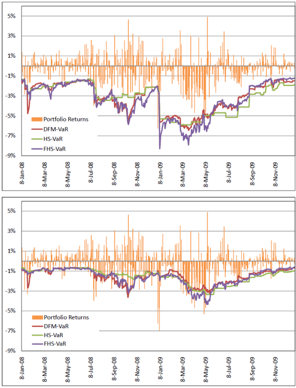
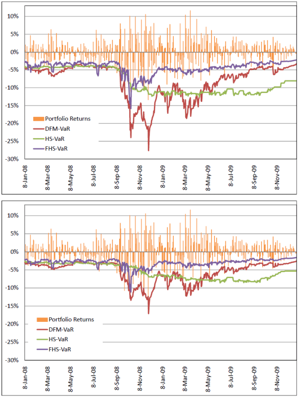
6.1.1 Descriptive Figures

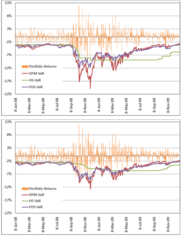
We begin the discussion of results by commenting on the time series plots of portfolio returns and VaR estimates in Figures 8.3 - 8.5. All DFM-VaRs in the figures are based on the case .¹⁵ The top panel in each figure displays the returns alongside the 99% VaRs, while the bottom panel displays returns alongside 95% VaRs. Figure 8.3 displays the return series and VaR estimates for the S&P 500 portfolio. Figure 8.4 displays the return series and VaR estimates for the Momentum portfolio. Figure 8.5 displays the return series and VaR estimates for the Money portfolio.

We first note that, as expected, across all model specifications and portfolios, the VaR associated with a higher confidence level is greater in absolute value and more volatile. We also observe that in general, the DFM-VaR is more responsive than the HS-VaR, and it is large in absolute values during periods of high market volatility.

As argued in Pritsker (2006), HS-VaR is often very stale and outdated, even static. As is evidenced in the figures, the estimates move to a different level only when a significant negative shock occurs and remain there until the shock passes through the sample time frame. A careful comparison of the graphs shows that the portfolio with most composition variation (Money) produces a more dynamic HS-VaR, compared to the S&P 500 and Momentum portfolios. Still, this level of variability is not sufficient to prevent the HS-VaR from being overly conservative for certain periods, and insufficiently conservative for others.

The FHS-VaR is more responsive than the HS-VaR, and it generally moves in the same direction as the DFM-VaR. In fact, for the S&P 500 and Momentum portfolios, FHS-VaR is quite similar to the DFM-VaR. However, for the Money portfolio, FHS-VaR displays levels that lead to frequent breaches. We argue that since the FHS ignores the correlation across risk factors it tends to underestimate risk for the Money portfolio, which exhibits high levels of negative skewness and volatility.

6.1.2 VaR Evaluation Tests

In support of the descriptive figures, we now provide more formal evaluations of all VaRs. To briefly summarize the results to follow, the DFM-VaRs perform well, particularly when compared to HS-VaR, and they are also computationally efficient. The FHS-VaR also has reasonable performance for two out of three portfolios, but it is very computationally burdensome.

Table 8.4 displays the properties and results from statistical tests for all VaR methodologies at the 99% confidence level. The three panels in the table correspond to the three test portfolios. In Panel A, we observe that for the S&P 500 portfolio the DFM-VaRs display very reasonable VaR breaches (1.4% for all three DFM-VaRs, when 1% is expected), while the HS-VaR displays the most (2.8%). FHS-VaR also performs well in terms of VaR breaches, but the size of the breaches are on average substantially higher. (1.03%, compared to 0.66% - 0.75% for DFM-VaRs).

The last two rows in each of the panels display the p-values associated with the the CaViaR and Quantile tests. For the S&P 500 portfolio, the CaViaR test suggests that the null that VaR breaches are independent across time and occurs 1% of the time unconditionally cannot be rejected at a 10% significance level for DFM-VaR with

. The null also cannot be rejected for FHS-VaR. Not surprisingly, the null is rejected for HS-VaR quite definitively. Turning to the Quantile test, we cannot reject the null that the VaR is the correct estimate of the conditional quantile, for all VaRs we consider.

Panel B presents the results for the Momentum portfolio. For this portfolio all VaRs experience too many breaches. FHS-VaR appears to perform the best in terms of breaches and average breach size, and two of the DFM-VaRs ( and ) experience similar performance as the FHS-VaR. The DFM-VaR when performs quite poorly, indicating that the modeling of serial correlation in the factors may not be appropriate for this portfolio. The CaViaR test suggests that all the VaR models are incorrectly specified. With the exception of the FHS-VaR, the Quantile test also suggests that all VaR estimates fail to capture the true conditional quantile. One could interpret these results as a challenge most methodologies face when dealing with strategies whose associated returns feature excessive negative skewness (see Table 8.3).

Recall that the Money portfolio exhibits the largest standard deviation compared to the other two portfolios. In Panel C, we see that the FHS-VaR has the most breaches and the HS-VaR has the large average breach sizes. It is somewhat surprising that the FHS-VaR performs so poorly for this portfolio, given the Money portfolio's similarities to the S&P 500 portfolio. The CaViaR test suggests that only the DFM-VaR when displays an acceptable performance at a 10% level, while it rejects all other VaRs at 10%, with particularly strong evidence of rejection for the FHS-VaR. Given its poor performance, it is not surprising that the FHS-VaR is the only VaR being rejected by the Quantile test at the 10% level.

Table 8.5 exhibits the performances of 95% VaRs. The table is structured in the same way as Table 8.4. At this confidence level, the number of breaches is higher for all VaRs as expected (ideally, a VaR should be breached 5% of the time), while the average breach size is typically lower, due to the fact there are many more smaller breaches compared to the 99% VaRs, which tend to be breached only by quite extreme returns. The rankings of the different VaR models at the 95% level are similar to those at the 99% level: the DFM-VaRs generally work well; the FHS-VaR has similar performances as the DFM-VaRs except for the Money portfolio; all VaRs perform relatively poorly for the Momentum portfolio; and the HS-VaR unambiguously performs the worst for the S&P 500 and Money portfolios.

Finally, Table 8.6 compares the average time required by each VaR model to compute one out-of-sample VaR.¹⁶ Not surprisingly, HS-VaR is the most computationally efficient, because it requires virtually no modeling. Compared to the FHS-VaR, the DFM-VaRs are highly efficient: while the FHS-VaR takes more than 17 minutes to calculate each VaR, due to the univariate GARCH filtering applied to the 3,376 stocks, the DFM-VaR has average computation time ranging from only 7 to 10 seconds per VaR. From a practical perspective, DFM-VaRs are highly efficient.

7 DFM-VaR for Individual Stocks

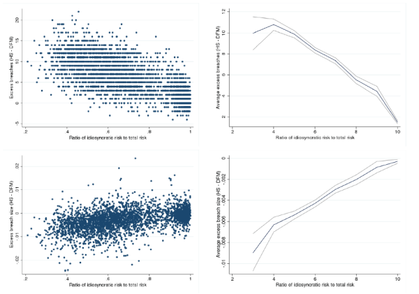
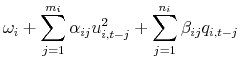
To the extent that large swings in individual stock prices are generated by systematic shocks, it appears that the DFM-VaR will be able to capture such movements through the extraction of systematic latent factors. Hence, we test whether the DFM-VaR produces better VaR estimates for stocks that have a higher proportion of systematic risk relative to total risk. Indeed, we find that the DFM-VaR generates fewer breaches for stocks with less idiosyncratic risk, relative to HS-VaR.

For each stock, we measure total risk as the variance of daily excess returns, and idiosyncratic risk as the variance of the residuals obtained by regressing daily excess returns on the following four factors: market, smb, hml, and momentum.¹⁷ The top panels of Figure 8.6 shows the number of breaches of the HS-VaR in excess of the DFM-VaR (when and ), both for individual stocks (top-left panel) and for portfolios of stocks with similar proportions of idiosyncratic risk (top-right panel). The average cumulative difference in the number of breaches (over 2008-2009) monotonically declines in statistically and economically significant terms with the proportion of idiosyncratic risk. In fact, for stocks with little systematic risk, there is little difference between the HS-VaR and DFM-VaR estimates.

The bottom panels of Figure 8.6 study the size of the VaR breaches against the proportion of idiosyncratic risk. The results show that for stocks that are more exposed to systematic risk, the difference between the average breach size of the DFM-VaR and HS-VaR is small. Careful inspection of the data shows that this happens because for such stocks, the HS-VaR is subjected to many more breaches than the DFM-VaR (see the top two panels of Figure 8.6), and many of these breaches are small in size. These small breaches bring down the average breach size. As we move to stocks that are less exposed to systematic risk, this difference disappears because the DFM-VaR and HS-VaR are subjected to more breaches common to both VaRs.

8 Conclusions

This paper introduces a VaR methodology suitable for trading portfolios that are driven by a large number of financial variables with time-varying volatilities. The use of Dynamic Factor Models (DFM) in VaR allows the risk manager to accurately account for time-varying volatilities and correlations with relatively small computational burden. We test the method on three stock portfolios and show that DFM-VaR compares favorably to VaRs based on Historical Simulation (HS-VaR) and Univariate Filtered Historical Simulation (FHS-VaR) in terms of back-testing breaches and average breach sizes. In addition, DFM-VaRs are shown to be computationally efficient.

We construct three test portfolios to test the DFM-VaR: one that replicates a broad market index, one based on the momentum effect with portfolio weights that change every month, and one that includes stocks more likely to experience large swings in prices, as proxied by the slope of the options implied volatility smile, with portfolio weights that change every day. The three test portfolios differ in terms of the features of their returns distributions. Our descriptive figures illustrate some of the well-known deficiencies of the commonly-used HS-VaR approach, most notably its inability to capture time-varying volatility. On the other hand, the DFM-VaR and FHS-VaR perform reasonably well in general, but the DFM-VaR clearly out-performs the FHS-VaR in one portfolio.

We use two statistical tests to evaluate the proposed DFM-VaR. These tests are based on Engle & Manganelli (2004) and Gaglianone et al. (2011). For the equally-weighted, time-invariant S&P 500 portfolio and the daily re-balancing Money portfolios, the evaluation tests suggest that the proposed DFM-VaR performs well. Because the Momentum portfolio is characterized by a high level of negative skewness, none of the models was able to estimate the VaR very accurately. Still, the DFM-VaR provides reasonable estimates for that portfolio.

To the extent that large swings in individual stock prices are generated by systematic shocks, it is possible that the DFM-VaR will able to capture such movements through the systematic latent factors extracted in the proposed procedure. Hence, as a robustness check, we test whether the DFM-VaR produces better VaR estimates for individual stocks that have a higher proportion of systematic risk relative to total risk. As expected, we find that the DFM-VaR generates fewer breaches for stocks with less idiosyncratic risk than HS-VaR.

In future work, we plan to investigate how DFM-VaR may be able model financial variables with richer time series dynamics, like price jumps. Such an extension would be useful when modeling portfolios of assets with non-linear payoffs, like options, or assets of a different class than stocks, such as tranched credit derivatives or interest rate swaptions.

Bibliography

L. Alessi, et al. (2009).

`Estimation and Forecasting in Large Datasets with Conditionally Heteroskedastic Dynamic Common Factors'.
ECB Working Paper.

C. Alexander (ed.) (2001).

Mastering Risk, vol. 2, chap. Orthogonal GARCH.
Financial Times - Prentice Hall.

C. Alexander (2002).

`Principal Component Models for Generating Large Covariance Matrices'.
Review of Banking, Finance and Monetary Economics, Economic Notes 31(2):337-359.

J. Bai (2003).

`Inferential Theory for Factor Models of Large Dimensions'.
Econometrica 71(1):135-171.

J. Bai & S. Ng (2006).

`Confidence Intervals for Diffusion Index Forecast and Inference with Factor-Augmented Regressions'.
Econometrica 74(3):1133-1150.

J. Bai & S. Ng (2007).

`Determining the Number of Primitive Shocks in Factor Models'.
Journal of Business and Economic Statistics 25(1):52-60.

G. Bakshi, et al. (2003).

`Stock Return Characteristics, Skew Laws, and the Differential Pricing of Individual Equity Options'.
The Review of Financial Studies 16(1):101-143.

G. Barone-Adesi, et al. (1999).

`VaR without Correlations for Nonlinear Portfolios'.
Journal of Futures Markets 19:583-602.

J. Berkowitz (2001).

`Testing Density Forecasts, With Applications to Risk Management'.
Journal of Business and Economic Statistics 14(4):465-474.

J. Berkowitz, et al. (2009).

`Evaluating Value-at-Risk Models with Desk-Level Data'.
Management Science, pp. 1-15.

J. Berkowitz & J. O'Brien (2002).

`How Accurate Are Value-at-Risk Models at Commercial Banks?'.
The Journal of Finance LVII(3):1093-1111.

J. Berkowitz & J. O'Brien (2006).

Risks of Financial Institutions, chap. Estimating Bank Trading Risk: A Factor Model Approach.
NBER.

P. F. Christoffersen & D. Pelletier (2004).

`Backtesting Value-at-Risk: A Duration Approach'.
Journal of Financial Economterics 2(1):84-108.

J. C. Cox, et al. (1985).

`A Theory of the Term Structure of Interest Rates'.
Econometrica 53(2):385-407.

J.-M. Dufour (2006).

`Monte Carlo Tests with Nuissance Parameters: A General Approach to Finite-Sample Inference and Nonstandard Asymptotics'.
Journal of Econometrics 133(2):433-477.

R. F. Engle (2002).

`Dynamic Conditional Correlation: A Simple Class of Multivariate Generalized Autoregressive Conditional Heteroskedasticity Models'.
Journal of Business and Economic Statistics 20(3):339-350.

R. F. Engle (2007).

`High Dimension Dynamic Correlations'.
Prepared for a Festchrift for David Hendry.

R. F. Engle & B. T. Kelly (2009).

`Dynamic Equicorrelation'.
NYU Working Paper.

R. F. Engle & K. Kroner (1995).

`Multivariate Simultaneous GARCH'.
Econometric Theory 11(5):122-150.

R. F. Engle & S. Manganelli (2004).

`CAViaR: Conditional Autoregresive Value at Risk by Regression Quantiles'.
Journal of Business and Economic Statistics 22(4):367-381.

R. F. Engle, et al. (2007).

`Fitting and Testing Vast Dimensional Time-Varying Covariance Models'.
NYU Working Paper.

R. F. Engle & K. Sheppard (2008).

`Evaluating the Specification of Covariance Models for Large Portfolios'.
NYU Working Paper.

E. F. Fama & K. R. French (1996).

`Multifactor Explanations of Asset Pricing Anomalies'.
Journal of Finance 51:55-84.

W. P. Gaglianone, et al. (2011).

`Evaluating Value-at-Risk Models via Quantile Regression'.
Journal of Business and Economic Statistics 29(1):150-160.

J. Hull & A. White (1998).

`Incorporating Volatility Updating into the Historical Simulation Method for VaR'.
Journal of Risk 1:5-19.

N. Jegadeesh & S. Titman (1993).

`Returns to Buying Winners and Selling Loosers: Implications for stock Market Efficiency'.
The Journal of Finance 48(1):65-91.

J. Kerkhof & B. Melenberg (2004).

`Backtesting for Risk-based Regulatory Capital'.
Journal of Banking and Finance 28:1845-1865.

P. Kupiec (1995).

`Techniques for Verifying the Accuracy of Risk Measurement Models'.
Journal of Derivatives 3:73-84.

J. Mincer & V. Zarnowitz (1969).

The Evaluation of Economic Forecasts and Expectations.
National Bureau of Economic Research, New York.

C. Perignon & D. R. Smith (2010).

`The Level and Quality of Value-at-Risk Disclosure by Commercial Banks'.
Journal of Banking and Finance 34:362-377.

M. Pritsker (2006).

`The Hidden Dangers of Historical Simulation'.
Journal of Banking and Finance 30:561-582.

J. H. Stock & M. W. Watson (2002).

`Macroeconomic Forecasting Using Diffusion Indexes'.
Journal of Business and Economic Statistics 20(2):147-162.

Table 8.1: Correlations of $f_{1t}$ and $f_{2t}$ with various asset pricing factors
	mkt	smb	hml	umd	dPut	dVix	$f_{1t}$	$f_{2t}$
mkt	1
smb	-0.07	1
hml	0.527	-0.02	1
umd	-0.63	-0.03	-0.71	1
dPut	0.89	-0.18	0.41	-0.48	1
dVix	-0.84	0.17	-0.36	0.44	-0.82	1
$f_{1t}$	-0.96	-0.18	-0.58	0.71	-0.81	0.77	1
$f_{2t}$	-0.09	0.35	0.22	-0.11	-0.15	0.16	0.00	1

Table shows correlations between selected asset pricing factors and the DFM-VaR factors. Mkt, smb, hml and umd are the Fama-French and momentum factors, while dPut is the arithmetic return on the PUT index provided by the CBOE, and dVix is the change in the implied volatility index VIX. $f_{1t}$ and $f_{2t}$ are the first two principal components extracted from the stock returns data set.

Table 8.2: Correlations during the height of the 2008 financial crisis
	mkt	smb	hml	umd	dPut	dVix	$f_{1t}$	$f_{2t}$
mkt	1
smb	-0.31	1
hml	0.50	-0.10	1
umd	-0.74	0.12	-0.75	1
dPut	0.91	-0.37	0.41	-0.58	1
dVix	-0.87	0.35	-0.34	0.57	-0.82	1
$f_{1t}$	-0.96	0.05	-0.56	0.80	-0.84	0.81	1
$f_{2t}$	-0.28	0.48	0.15	0.19	-0.34	0.36	0.19	1

Table 8.3: Summary statistics for portfolio returns
	S&P 500	Momentum	Money
Mean	0.01%	-0.34%	-0.05%
Std. Dev.	2.51%	1.49%	3.38%
Skewness	1.68%	-46.59%	-13.07%
Kurtosis	617.15%	505.48%	486.64%

Table shows summary statistics for the three portfolios described in section 5. Unwinsorized returns data on 3,376 individual stocks are used to calculate portfolio summary statistics over 750 trading days in 2007 - 2009.

Table 8.4: 99% VaR comparisons across portfolios. Panel A: *S&P 500* Portfolio
	DFM-VaR	DFM-VaR	DFM-VaR	HS-VaR	FHS-VaR
Breach %	1.40%	1.40%	1.40%	2.80%	1.20%
Avg. breach size	0.75%	0.75%	0.66%	1.17%	1.03%
CaViaR p-value	10.09%	8.35%	20.48%	0.60%	85.56%
Quantile test p-value	51.73%	68.48%	88.83%	44.33%	95.14%

Table 8.4: 99% VaR comparisons across portfolios. Panel B: *Momentum* Portfolio
	DFM-VaR	DFM-VaR	DFM-VaR	HS-VaR	FHS-VaR
Breach %	2.60%	2.40%	7.80%	2.80%	2.40%
Avg. breach size	1.25%	1.35%	1.24%	1.33%	1.17%
CaViaR p-value	0.05%	0.05%	0.05%	0.05%	0.05%
Quantile test p-value	1.55%	8.17%	0.01%	4.71%	15.45%

Table 8.4: 99% VaR comparisons across portfolios. Panel C: *Money* Portfolio
	DFM-VaR	DFM-VaR	DFM-VaR	HS-VaR	FHS-VaR
Breach %	1.60%	1.40%	1.60%	2.00%	8.60%
Avg. breach size	0.91%	1.00%	0.85%	1.76%	1.69%
CaViaR p-value	5.70%	11.29%	7.55%	2.00%	0.05%
Quantile test p-value	42.91%	46.65%	65.96%	27.01%	9.72%

Panel A: S&P 500 Portfolio

Table 8.5: 95% VaR comparisons across portfolios.
	DFM-VaR	DFM-VaR	DFM-VaR	HS-VaR	FHS-VaR
Breach %	4.80%	5.60%	5.00%	6.60%	4.20%
Avg. breach size	0.91%	0.82%	0.98%	1.77%	0.97%
CaViaR p-value	53.97%	29.69%	47.93%	0.15%	49.88%
Quantile test p-value	68.51%	97.99%	56.61%	0.82%	20.55%

Table 8.5: 95% VaR comparisons across portfolios. Panel B: *Momentum* Portfolio
	DFM-VaR	DFM-VaR	DFM-VaR	HS-VaR	FHS-VaR
Breach %	16.00%	14.20%	21.80%	15.80%	14.80%
Avg. breach size	0.85%	0.85%	1.10%	0.98%	0.80%
CaViaR p-value	0.05%	0.05%	0.05%	0.05%	0.05%
Quantile test p-value	0.57%	0.20%	0.00%	0.00%	0.01%

Table 8.5: 95% VaR comparisons across portfolios. Panel C: *Money* Portfolio
	DFM-VaR	DFM-VaR	DFM-VaR	HS-VaR	FHS-VaR
Breach %	5.80%	5.80%	6.00%	7.20%	15.60%
Avg. breach size	1.13%	1.15%	1.27%	2.12%	1.96%
CaViaR p-value	24.69%	27.89%	64.67%	0.10%	0.10%
Quantile test p-value	46.41%	62.12%	48.68%	0.68%	0.00%

Table shows statistics on competing VaR models, across the three test portfolios. All VaRs are estimated using a 250 days rolling historical window, using methods described sections 4 and 6.1. "Breach %" is the percentage of days (out of 500 trading days in 2008-2009) for which realized portfolio returns breached the 95% VaR. "Avg. breach size" is the average of the sizes of the breaches over the 500 days. "CaViaR p-value" is the Monte Carlo based p-value (using 2000 replications) of the CaViaR test statistics described in section 6. "Quantile p-value" is the p-value of the Quantile test statistics with respect to a Chi-squared distribution with two degrees of freedom, as described in section 6.

Table 8.6: Average computation time for VaRs
	DFM-VaR	DFM-VaR	DFM-VaR	HS-VaR	FHS-VaR
Comp. Time	7.1 secs	8.2 secs	9.8 secs	0.5 secs	17.6 mins

Table shows computation time required by different VaR models. "Comp. Time" is the average computation time it takes to calculate one VaR, across the 500 out-of-sample VaRs calculated. The same Matlab server is used to compute all VaRs, and all VaRs are computation began at the same time.

Figure: 8.1 Plot of $f_{1t}$ and $f_{2t}$

The graphs display the time series of the first two principal components extracted from the stock returns data set (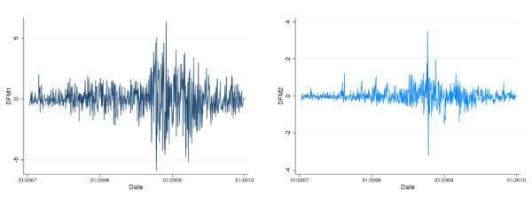 $f_{1t}$ on the left, $f_{2t}$ on the right). 2007-2009.

Figure: 8.2 Plot of $f_{1t}$ , $f_{2t}$ and the `mkt' and `smb' factors

The left panel shows the market factor against $f_{1t}$ , while the right panel shows smb against $f_{2t}$ . 2007-2009.

Figure: 8.3 Returns and VaRs for the *S&P 500* portfolio. 99% VaRs in top graph; 95% VaRs in bottom graph.

Figure: 8.4 Returns and VaRs for the *Momentum* portfolio. 99% VaRs in top graph; 95% VaRs in bottom graph.

Figure: 8.5 Returns and VaRs for the *Money* portfolio. 99% VaRs in top graph; 95% VaRs in bottom graph.

Figure: 8.6 Idiosyncratic risk and the number and size of exceptions

Idiosyncratic risk is the variance of the residuals from stock-specific regressions of daily excess returns on the Market, Smb, Hml and Umd factors. Total risk is the variance of excess returns. The ratio of idiosyncratic risk to total risk is the former divided by the latter. The ten buckets of idiosyncratic risk have a thickness of 0.1, from 0 to 1. Stocks with the highest idiosyncratic risk belong to bucket 10. The regressions are based on daily excess returns, and cover the 2008-2009 period. The left panels plots the "Excess breaches"(top) and "Excess breach size" (bottom) for individual stocks, on the amount of idiosyncratic risk. Excess number (size) is defined as the number (average size) of HS-VaR breaches minus the number (average size) of DFM-VaR breaches. The right panels reports the average, across stocks within a given bucket, of the excess number and size of breaches shown in the left panels. The 95% confidence intervals are calculated from the percentiles of the distribution of the averages within each bucket, whereas the distribution is based on 1,000 bootstrap replications. Note that the left and right panels have different scales.

Footnotes

* This article represents the views of the authors and should not be interpreted as reflecting the views of the Board of Governors of the Federal Reserve System or other members of its staff. Return to Text

** Corresponding author: [email protected] Return to Text

1. FHS-VaR can also be implemented through multivariate filtering, with, for instance, multivariate GARCH models, but the estimation becomes difficult as the dimensionality of the problem increases (Engle et al. (2007)). Return to Text

2. The methodology can be easily generalized to a holding period of

. Return to Text

3. When implementing a VaR model, risk managers often only use information that goes back

periods, from

. For instance, the 1996 Market Risk Amendment to the Basel Accord allows the use one year of past data (or $R\approx 250$ business days). Return to Text

4. $\theta_{T+1}$ usually includes portfolio weights or pricing model parameters, which the risk manager knows at

. Return to Text

5. See, for example, the work by Barone-Adesi et al. (1999), and Pritsker (2006) Return to Text

6. This form is also known as the Static Form in the DFM literature. Return to Text

7. There is a literature that offers techniques on estimating

and

, see Bai & Ng (2007), for instance. Return to Text

8. We use Kevin Sheppard's codes for DCC estimation, available at www.kevinsheppard.com. Return to Text

9. The option pricing data is obtained from Optionmetrics, and we only consider options with a non-zero trading volume, standard settlement, positive bid and ask prices, and for which the ask is greater than the bid. Return to Text

10. On a few days we are unable to calculate smile slopes due to limited data availability, and we use the weights of the immediately preceding days. Return to Text

11. The 1996 Market Risk Amendment of the Basel Accord imposes a regulatory capital multiplier that depends on the number of VaR breaches experienced over the past year. Return to Text

12. For time-varying portfolios, both the realized returns of a portfolio and its VaRs are essentially nonstationary. Techniques proposed in the literature to evaluate VaR for time-varying portfolios include Berkowitz (2001) and Kerkhof & Melenberg (2004). These procedures, however, are more suitable when the forecast distribution of returns are parametric, whereas the VaRs we are interested in are all either semiparametric (DFM-VaR and FHS-VaR) or nonparametric (HS-VaR). Berkowitz (2001) is appropriate when one is interested in testing the accuracy of the entire distribution, rather than just the VaR. Return to Text

13. Simple calculations show this continues to hold even when the portfolio is time-varying. Return to Text

14. 99% VaRs are typically used by financial institutions for regulatory capital purposes, while 95% VaRs are often used for internal risk management purposes. Return to Text

15. The plots for the cases of

and

are similar, and are available upon request. Return to Text

16. Note that the portfolio for which the VaRs are computed generally do not affect computational time, because the portfolio weights for all three portfolios are matrices with the same dimension. Return to Text

17. The factor data were collected from the Fama-French section of the WRDS database. Return to Text

^♣ This version is optimized for use by screen readers. Descriptions for all mathematical expressions are provided in LaTex format. A printable pdf version is available. Return to Text

Dynamic Factor Value-at-Risk for Large, Heteroskedastic Portfolios*

Bibliography

Dynamic Factor Value-at-Risk for Large,
Heteroskedastic Portfolios*