
Investment, Idiosyncratic Risk, and Ownership
Keywords: Investment, idiosyncratic risk, managerial ownership, risk aversion
Abstract:
In frictionless capital markets, only the systematic component of risk is relevant for investment decisions. By contrast, idiosyncratic risk should not affect the valuation of investment projects, as long as firm owners are diversified and managers maximize shareholder value. However, the data indicate that there is a significant negative relation between idiosyncratic risk and investment for publicly traded firms in the United States. In addition, executives in publicly traded firms across the world hold a substantial stake in their firms, consistent with the predictions of agency theory. Combining these two observations suggests that, since investment decisions are undertaken by managers on behalf of shareholders, poorly diversified managers may cut back on investment when uncertainty about the firm's future prospects increases, even if this uncertainty is specific to the firm.
In this paper we argue that managerial risk aversion induces a negative relation between idiosyncratic volatility and investment. We find that the negative relation between investment and idiosyncratic risk is stronger when managers own a larger fraction of the firm. This difference in investment-risk sensitivities across firms is economically large. For instance, idiosyncratic uncertainty increased during the 2008 to 2009 financial crisis. During this period, firms with higher fractions of insider ownership reduced investment by 8% of their existing capital stock, compared to 2% for firms with a more diversified shareholder base.
Our results suggest that forcing managers to bear firm-specific risk induces a wedge between manager and shareholder valuations of investment opportunities and may lead to underinvestment from the perspective of well-diversified shareholders. Shareholders can mitigate this effect through effective monitoring or by providing a convex compensation scheme using stock option grants. We find that the effect of insider ownership on the investment-risk relation is weaker for firms with higher levels of institutional ownership. This is consistent with the notion that institutional investors are more effective monitors than individual shareholders. In addition, we find that, controlling for the level of insider ownership, firms with more convex compensation contracts, which therefore increase in value with uncertainty, have lower investment-risk sensitivity. In fact, proponents of option-based compensation have used this argument to justify providing executives with downside protection as a compromise between supplying incentives and mitigating risk-averse behavior.
We estimate firm-specific risk using stock return data, where we decompose stock return volatility into a systematic component and an idiosyncratic component. Our first concern is that idiosyncratic volatility is endogenous and could be correlated with the firm's investment opportunities. If
Tobin's ![]() is an imperfect measure of investment opportunities, this would lead to omitted variable bias. We address this issue by considering alternative measures of growth opportunities, as
well as estimation methods that directly allow for measurement error in Tobin's
is an imperfect measure of investment opportunities, this would lead to omitted variable bias. We address this issue by considering alternative measures of growth opportunities, as
well as estimation methods that directly allow for measurement error in Tobin's ![]() . In addition, we instrument for idiosyncratic risk with a measure of the firm's customer base concentration.
Our intuition is that firms selling to only a few customers are less able to diversify demand shocks for their product across customers and thus will be riskier. We find that idiosyncratic volatility remains a statistically significant predictor of investment, even after addressing these
endogeneity concerns. We consider this to be evidence supportive of a causal relation from idiosyncratic risk to investment.
. In addition, we instrument for idiosyncratic risk with a measure of the firm's customer base concentration.
Our intuition is that firms selling to only a few customers are less able to diversify demand shocks for their product across customers and thus will be riskier. We find that idiosyncratic volatility remains a statistically significant predictor of investment, even after addressing these
endogeneity concerns. We consider this to be evidence supportive of a causal relation from idiosyncratic risk to investment.
Our second main concern is that insider ownership is endogenous and could be correlated with firm characteristics that might be affecting the investment-uncertainty relation. For instance, insider ownership may be correlated with costs of external finance: if a firm is unable to attract outside investors, then insiders will be forced to hold a substantial stake in the firm. In this case, convex costs of external finance will lead to a negative relation between firm-specific uncertainty and investment through a precautionary saving motive. Alternatively, insider ownership may be correlated with the degree of industry competition, since a competitive product market could serve as a substitute for high-powered incentives. Imperfect competition may then affect the investment-uncertainty relation through the convexity of the marginal product of capital. We address these concerns by comparing the investment of firms with different levels of insider ownership but with similar size, financial constraints, market power, industry competition, and degree of investment irreversibility. Controlling for these firm characteristics, we find that firms with higher insider ownership display higher sensitivity of investment to idiosyncratic risk.
The rest of the paper is organized as follows. Section I reviews the related research. Section II provides a simple model illustrating how idiosyncratic risk can affect capital investment. Section III documents empirically the negative relation between idiosyncratic risk and investment. Section IV shows how this relation varies with levels of insider ownership, convexity of executive compensation schemes, and institutional ownership. Section V addresses concerns about endogeneity of idiosyncratic volatility and insider ownership. Section VI explores whether our results hold out of sample, particularly during the financial crisis of 2008 to 2009. Section VII concludes. Details on data construction are delegated to the Appendix.
1 Related Research
In traditional economic theory, there is no role for managerial characteristics in firm decisions. However, several recent papers provide empirical evidence to the contrary. Bertrand and Schoar (2003) find a role for managerial fixed effects in corporate decisions. Malmendier and Tate (2005) construct a measure of overconfidence based on the propensity of CEOs to exercise options early and find greater investment-cashflow sensitivity in firms with overconfident CEOs. Using psychometric tests administered to corporate executives, Graham, Harvey, and Puri (2010) show that traits such as risk aversion, impatience, and optimism are related to corporate policies.
Various studies indicate that the identity of a firm's shareholders may be important. Himmelberg, Hubbard, and Love (2002) document that, even in publicly traded firms, insiders hold a substantial share of the firm. In a cross-country analysis, they find that countries with higher levels of investor protection are characterized by lower levels of insider ownership. Admati, Pfleiderer, and Zechner (1994) illustrate theoretically that large investors exert monitoring effort in equilibrium, even when monitoring is costly. Gillan and Starks (2000) and Hartzell and Starks (2003) provide empirical evidence supporting the view that institutional ownership can lead to more effective corporate governance.
The theoretical research in real options has extensively examined the sign of the relation between investment and total uncertainty. The theoretical conclusions are rather ambiguous, as the sign depends, among other things, on assumptions about the production function, the market structure, the shape of adjustment costs, the importance of investment lags, and the degree of investment irreversibility. An incomplete list includes Hartman (1972), Abel (1983), and Caballero (1991). More recently, Chen, Miao, and Wang (2010) and DeMarzo et al. (2010) explore the effect of managerial risk aversion and idiosyncratic risk on investment decisions in dynamic models. The previous papers focus on the firm's partial equilibrium problem, while Angeletos (2007) and Bloom (2009) investigate the general equilibrium effects of an increase in uncertainty on investment.
Most of these theoretical papers make no distinction between idiosyncratic and systematic uncertainty. By contrast, we differentiate between idiosyncratic and systematic uncertainty, because managers can hedge exposure to systematic but not to idiosyncratic risk. For instance, Knopf, Nam, and Thornton (2002) find that managers are more likely to use derivatives to hedge systematic risk when the sensitivity of their stock and stock option portfolios to stock price is higher and the sensitivity of their option portfolios to stock return volatility is lower.
Several empirical studies explore the predictions of real option models. An incomplete list includes Leahy and Whited (1996), Guiso and Parigi (1999), Bond and Cummins (2004), Bulan (2005), and Bloom, Bond, and VanReenen (2007). With the exception of Bulan (2005), these papers focus on the relation between investment and total or systematic uncertainty facing the firm. This branch of research mostly finds a negative relation between uncertainty and investment, though results appear to be somewhat sensitive to the estimation method. We contribute to this research by showing that managerial risk aversion may be an important channel behind the investment-uncertainty relation.
2 Model
Here we propose a simple two-period model that demonstrates how idiosyncratic risk can affect capital investment in the absence of adjustment costs or other investment frictions. We abstract from such frictions because we are interested in a different channel: investment decisions are taken by risk-averse managers who hold undiversified stakes in their firm. We focus on the idiosyncratic rather than the total uncertainty facing the firm because, as long as managers have access to the same hedging opportunities as shareholders, the presence of systematic risk need not lead to distorted investment decisions from the shareholders' perspective. By contrast, since top executives are not permitted to buy put options or short their own company's stock, they cannot hedge away their exposure to firm-specific risk. Thus, idiosyncratic risk introduces a wedge between managers' and shareholders' optimal decisions.
A firm starts with cash ![]() at
at ![]() and produces output at
and produces output at ![]() according to
according to
where
The manager owns a fraction ![]() of the firm, while the remaining shares are held by shareholders who are risk averse but hold the market portfolio. We assume that the manager cannot
diversify his stake in the firm. The manager derives utility from consumption
of the firm, while the remaining shares are held by shareholders who are risk averse but hold the market portfolio. We assume that the manager cannot
diversify his stake in the firm. The manager derives utility from consumption ![]() and disutility from effort
and disutility from effort ![]() :
:
Utility over consumption takes the form
The manager's contract consists of a choice of ownership, ![]() , and an initial transfer,
, and an initial transfer, ![]() . Given the contract, the manager will then choose how much to invest in capital,
. Given the contract, the manager will then choose how much to invest in capital, ![]() , how much effort to provide,
, how much effort to provide, ![]() , and how much to save in the riskless asset,
, and how much to save in the riskless asset, ![]() , to maximize ( 2), subject to ( 1) and the two following budget constraints:
, to maximize ( 2), subject to ( 1) and the two following budget constraints:
We assume that the principal cannot write contracts on
PROPOSITION 1: The manager's optimal choice of capital, ![]() , bonds,
, bonds, ![]() , and effort,
, and effort, ![]() , are such that
, are such that
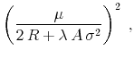
The elasticity of investment to idiosyncratic risk is
 |
(8) |
and is decreasing in
The first thing to note is that, as long as ![]() , the manager will underinvest from the perspective of the shareholders, who are diversified and thus behave as if risk neutral with
respect to X. Their optimal capital choice equals
, the manager will underinvest from the perspective of the shareholders, who are diversified and thus behave as if risk neutral with
respect to X. Their optimal capital choice equals
![]() . By contrast, the manager holds an undiversified stake in the firm, and therefore his choice of capital stock will depend on the level of the
idiosyncratic risk of the firm,
. By contrast, the manager holds an undiversified stake in the firm, and therefore his choice of capital stock will depend on the level of the
idiosyncratic risk of the firm, ![]() .
.
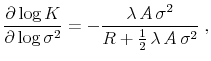
If ![]() were optimally chosen, it would depend, among other things, on the level of idiosyncratic risk and on the manager's risk aversion and cost of effort.1 When the principal chooses
were optimally chosen, it would depend, among other things, on the level of idiosyncratic risk and on the manager's risk aversion and cost of effort.1 When the principal chooses ![]() , she faces a tradeoff:
increasing
, she faces a tradeoff:
increasing ![]() induces higher effort on the part of the manager, but also leads to underinvestment, since the manager is risk averse. This is similar to the classic incentives versus
insurance tradeoff. The difference here lies in the cost of providing incentives. For instance, in Holmström (1979) the cost of providing incentives is simply the utility cost to the agent, whereas here there is an additional cost, namely, underinvestment in capital.
induces higher effort on the part of the manager, but also leads to underinvestment, since the manager is risk averse. This is similar to the classic incentives versus
insurance tradeoff. The difference here lies in the cost of providing incentives. For instance, in Holmström (1979) the cost of providing incentives is simply the utility cost to the agent, whereas here there is an additional cost, namely, underinvestment in capital.
In the following sections, we investigate two testable implications of the model:
- PREDICTION 1: Firm-level investment displays a negative relation with idiosyncratic risk.
- PREDICTION 2: The negative relation between investment and idiosyncratic risk is stronger for firms with higher levels of insider ownership.
In our empirical results we take the variation in insider ownership as given. In reality, there are many reasons why shares of insider ownership may vary across firms. The concern would then be that ![]() varies endogenously with some unobservable firm characteristics that are actually responsible for the negative investment-risk relation. A first candidate is risk aversion. We can obtain some intuition from the model regarding the effect of risk aversion on the endogeneity of
varies endogenously with some unobservable firm characteristics that are actually responsible for the negative investment-risk relation. A first candidate is risk aversion. We can obtain some intuition from the model regarding the effect of risk aversion on the endogeneity of
![]() . Given that we do not observe the manager's risk aversion, our results will be biased toward rejecting the second prediction, even if the model is true. For instance, suppose that
. Given that we do not observe the manager's risk aversion, our results will be biased toward rejecting the second prediction, even if the model is true. For instance, suppose that
![]() is exactly inversely proportional to
is exactly inversely proportional to ![]() , so that less risk-averse managers
are given higher stakes in the firm. Then the investment-risk relation will be flat along levels of insider ownership.
, so that less risk-averse managers
are given higher stakes in the firm. Then the investment-risk relation will be flat along levels of insider ownership.
There are, however, some additional candidates that are outside the model. Insider ownership may be correlated with the degree of financial constraints, or it could be endogenously related to the level of competition in the product market. In Sections V.B and V.C we explore these possibilities in more detail.
3 Investment and Idiosyncratic Risk
In this section we examine the first prediction of our model, namely, the response of investment to the volatility of idiosyncratic risk, controlling for several factors that might affect this relation.
3.1 Data and Implementation
We construct our baseline measure of idiosyncratic volatility using weekly data on stock returns from CRSP.2 To estimate a firm's
idiosyncratic risk, we need to remove systematic risk factors that the manager can insure against. Therefore, for every firm ![]() and every year
and every year ![]() , we regress the firm's return on the value-weighted market portfolio,
, we regress the firm's return on the value-weighted market portfolio, ![]() , and on the corresponding value-weighted industry
portfolio,
, and on the corresponding value-weighted industry
portfolio, ![]() , based on the Fama and French (1997) 30-industry classification.
, based on the Fama and French (1997) 30-industry classification.
Our measure of yearly idiosyncratic investment volatility for firm ![]() is the volatility of the residuals across the 52 weekly observations. Thus, we decompose the total weekly return of a firm
is the volatility of the residuals across the 52 weekly observations. Thus, we decompose the total weekly return of a firm ![]() into a market-, industry-, and firm-specific or idiosyncratic component as
follows:
into a market-, industry-, and firm-specific or idiosyncratic component as
follows:
where
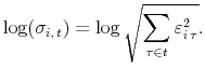
Our measure of idiosyncratic risk is highly persistent, even though it is constructed using a non-overlapping window: The pooled autocorrelation of
We estimate the response of investment to idiosyncratic risk using the following reduced-form equation:
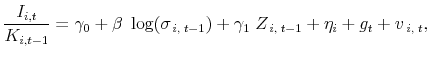
where the dependent variable is the firm's investment rate (
Our sample includes all publicly traded firms in Compustat over the period 1970 to 2005, excluding firms in the financial (SIC code 6000-6999), utilities (SIC
code 4900-4949), and government-regulated industries (SIC code >9000). We also
drop firm-year observations with missing SIC codes, with missing values for investment, Tobin's ![]() , cashflows, size, leverage, stock returns, and with negative book values of capital. We also
drop firms with fewer than 40 weekly observations in that year. Our sample includes a total of 104,646 firm-year observations. Finally, to eliminate the effect of outliers, we winsorize our data by year at the 0.5% and 99.5% levels in all specifications.
, cashflows, size, leverage, stock returns, and with negative book values of capital. We also
drop firms with fewer than 40 weekly observations in that year. Our sample includes a total of 104,646 firm-year observations. Finally, to eliminate the effect of outliers, we winsorize our data by year at the 0.5% and 99.5% levels in all specifications.
3.2 Effect of Idiosyncratic Risk on Investment
Our estimates of equation (11) are reported in Table I. The first column shows that when we include only idiosyncratic volatility and firm fixed effects, the coefficient on idiosyncratic volatility is ![]() and statistically significant. The second column presents the results of the benchmark estimation for equation (
and statistically significant. The second column presents the results of the benchmark estimation for equation (
![]() ), in which case the coefficient on idiosyncratic volatility is
), in which case the coefficient on idiosyncratic volatility is ![]() and statistically significant. In the third column we allow the time effects to vary by industry so as to capture any unobservable component varying at the industry level. In this case, identification comes from differences between a firm and its industry peers.
To keep the number of fixed effects manageable, we use the two-digit SIC classification. In this specification, the coefficient on log(
and statistically significant. In the third column we allow the time effects to vary by industry so as to capture any unobservable component varying at the industry level. In this case, identification comes from differences between a firm and its industry peers.
To keep the number of fixed effects manageable, we use the two-digit SIC classification. In this specification, the coefficient on log(
![]() ) remains mostly unaffected at
) remains mostly unaffected at ![]() .
.
Our estimates imply that the sensitivity of investment to idiosyncratic risk is economically significant. The standard deviation of log idiosyncratic volatility in our sample is 49%, so a
one-standard deviation increase in
![]() is associated with a
is associated with a ![]() to
to ![]() decrease in the investment-capital ratio. This is a substantial drop, as the mean investment-capital ratio in our sample is approximately 10%.
decrease in the investment-capital ratio. This is a substantial drop, as the mean investment-capital ratio in our sample is approximately 10%.
One concern is that idiosyncratic volatility may be positively correlated with systematic volatility, and thus the negative coefficient on idiosyncratic volatility may simply capture the effect of time variation in systematic risk premia on investment. To address this issue, we include lagged
systematic volatility as an additional regressor in the fourth column of Table I.3 The coefficient on idiosyncratic volatility is still negative and
significant (![]() ), whereas the coefficient on systematic volatility is positive and significant (0.6%). The coefficient on systematic volatility is economically small. Given that the
standard deviation of systematic volatility is 73% in the sample, these estimates imply that a one-standard deviation increase in systematic volatility is associated with a
), whereas the coefficient on systematic volatility is positive and significant (0.6%). The coefficient on systematic volatility is economically small. Given that the
standard deviation of systematic volatility is 73% in the sample, these estimates imply that a one-standard deviation increase in systematic volatility is associated with a ![]() increase in the investment-capital ratio.
increase in the investment-capital ratio.
The positive sensitivity of investment to systematic volatility might seem puzzling. All else equal, an increase in systematic volatility increases the firm's cost of capital and therefore should lead to a decrease in investment. Here, note that our measure of systematic volatility depends on
the firm's systematic risk exposures (beta) as well as the amount of market risk (market and industry volatility). Hence, our results are consistent with Bloom (2009), who finds a negative relation between investment and the volatility of the market portfolio. Furthermore, a firm's exposure to
systematic risk depends on its asset mix between investment opportunities and assets in place. In general, growth opportunities have greater exposure to systematic risk than assets in place, and hence firms with better investment opportunities will have higher systematic risk and also invest more
on average (for example, see Kogan and Papanikolaou (2010a)). If Tobin's ![]() is not a perfect measure of investment opportunities, the resulting omitted variable problem could bias our results
toward a positive coefficient on systematic volatility. We explore this possibility in Section V.A.
is not a perfect measure of investment opportunities, the resulting omitted variable problem could bias our results
toward a positive coefficient on systematic volatility. We explore this possibility in Section V.A.
4 Managerial Ownership and Risk Aversion
In this section we explore the second prediction of our model, namely, that the effect of idiosyncratic risk on investment is stronger for firms where managers hold a larger share in the firm. We also examine two related predictions that are outside the model.
First, over the last 20 years, several firms have switched to option-based compensation. Compensating executives with options, rather than shares, provides managers with a convex payoff whose value increases in the volatility of the firm. Thus, all else equal, increasing the convexity of the compensation package should mitigate the effect of risk aversion on investment (Ross (2004)). We test this prediction by examining the investment-risk sensitivity for firms with different levels of convexity in their compensation schemes. We expect that the negative effect of idiosyncratic risk on investment will be smaller for firms with more convex compensation schemes.
Second, if the investment-risk relation is due to poor managerial diversification, then managers are possibly destroying shareholder value by turning down high idiosyncratic risk but positive net present value projects. To mitigate this loss in value, shareholders may start monitoring managerial investment decisions. However, monitoring requires expertise and is costly, and hence, due to free-riding problems, small investors are unlikely to act as effective monitors. By contrast, institutional investors own large blocks of a firm's shares, and they have an incentive to develop specialized expertise in monitoring investment decisions. Therefore, if institutional investor ownership is correlated with corporate governance, we expect to find a weaker effect of insider ownership on the investment-uncertainty relation in firms with higher institutional ownership.
4.1 Insider Ownership
In this section we examine how investment-risk sensitivity varies with ownership by insider managers. We expect that investment will be more sensitive to idiosyncratic risk in firms where managers hold a larger fraction of the firm's shares.
Our source of managerial ownership data is the Thomson Financial Institutional Holdings database of filings derived from Forms ![]() , and
, and ![]() , over the period 1986 to 2005. We take as our measure of insider ownership in year
, over the period 1986 to 2005. We take as our measure of insider ownership in year ![]() the
reported yearly holdings of a firm's shares held by firm officers at the end of that year or at the latest filing date, as a fraction of the shares outstanding in the firm. After dropping missing and zero ownership values, the sample consists of
the
reported yearly holdings of a firm's shares held by firm officers at the end of that year or at the latest filing date, as a fraction of the shares outstanding in the firm. After dropping missing and zero ownership values, the sample consists of ![]() firm-year observations.
firm-year observations.
Table II presents summary statistics for firms with different levels of insider ownership. Every year, we sort firms into quintiles based on their lagged level of insider ownership. We report time-series averages of the median firm characteristic within ownership quintiles. The median level of
insider ownership across the five groups varies from ![]() to
to ![]() . The firms
with high levels of insider ownership tend to be smaller growth firms. They tend to have higher Tobin's
. The firms
with high levels of insider ownership tend to be smaller growth firms. They tend to have higher Tobin's ![]() , be more profitable, and invest more on average. In addition, they seem to be more
likely to face high costs of external finance: they have lower financial leverage, lower ratios of physical capital to book assets, and higher levels of the Whited and Wu (2006) index of financial constraints. Finally, firms with high insider ownership tend to have lower market power, as evidenced
by their lower level of sales as a fraction of the industry total.
, be more profitable, and invest more on average. In addition, they seem to be more
likely to face high costs of external finance: they have lower financial leverage, lower ratios of physical capital to book assets, and higher levels of the Whited and Wu (2006) index of financial constraints. Finally, firms with high insider ownership tend to have lower market power, as evidenced
by their lower level of sales as a fraction of the industry total.
We investigate how the investment-uncertainty relation varies with the degree of insider ownership by estimating equation (11) separately for firms in different insider ownership quintiles. Table III presents the results using our benchmark measure of insider ownership (columns one and two), as well as our ownership measure adjusted for executive option holdings (columns three and four; see Section IV.B and the Appendix for details).
The difference in the sensitivity of investment to idiosyncratic risk between the first and the fifth insider ownership quintiles ranges from ![]() to
to ![]() , depending on controls, and is statistically significant, with p-values ranging from 0.022 to 0.066. The dispersion in sensitivities is economically significant: for firms with high levels of insider ownership, a one-standard deviation increase in log
idiosyncratic volatility is associated with a drop of
, depending on controls, and is statistically significant, with p-values ranging from 0.022 to 0.066. The dispersion in sensitivities is economically significant: for firms with high levels of insider ownership, a one-standard deviation increase in log
idiosyncratic volatility is associated with a drop of ![]() to
to ![]() in
investment-capital ratios, compared to the group mean of 12%. By contrast, for firms with low insider ownership the effect is small in magnitude and not statistically significant: a
one-standard deviation increase in log idiosyncratic volatility is associated with a drop of
in
investment-capital ratios, compared to the group mean of 12%. By contrast, for firms with low insider ownership the effect is small in magnitude and not statistically significant: a
one-standard deviation increase in log idiosyncratic volatility is associated with a drop of ![]() to
to ![]() in investment-capital ratios, compared to the group mean of 9%.
in investment-capital ratios, compared to the group mean of 9%.
Our results here indicate that the investment-uncertainty relation varies with the level of insider ownership. This evidence is consistent with the view that the investment-risk relation is due at least in part due to poor managerial diversification. However, insider ownership is endogenous, and thus may be correlated with various other firm characteristics. We explore this possibility in detail in Sections V.B and V.C.
4.2 Option-Based Compensation
The previous section focuses on ownership by insiders in the form of shares in the firm, which exposes the manager to both profits and losses. An alternative form of ownership gives the manager call options on the firm's shares, which allow the executive to participate in gains but not losses. Due to the convex shape of the payoff function, an executive who is mostly compensated with options rather than with shares will effectively be less risk averse, and in fact he may even be risk loving in some regions. Consequently, we expect that investment will be less sensitive to idiosyncratic volatility in firms with more convex executive compensation schemes.
We use data on CEO option grants from Execucomp and the Black-Scholes option pricing model, adjusted for dividends, to compute the partial derivatives with respect to stock return volatility (![]() ) and stock price (
) and stock price (![]() ). For a given option scheme, the two variables of interest are
). For a given option scheme, the two variables of interest are
![]() and
and
![]() , where
, where ![]() is the number of options granted. The first variable
measures the change in the executive compensation scheme per unit increase in idiosyncratic volatility. The second variable measures the change in the executive compensation scheme per unit increase in the underlying stock price.
is the number of options granted. The first variable
measures the change in the executive compensation scheme per unit increase in idiosyncratic volatility. The second variable measures the change in the executive compensation scheme per unit increase in the underlying stock price.
Ross (2004) shows that simply granting an executive more call options does not necessarily make him less risk averse. The reason is that there is an offsetting effect coming from the option's delta, or its sensitivity to stock price changes. Thus, to investigate the effect of increased convexity
in executive compensation schemes, it is necessary to control for the level of ownership. We adjust the ownership measures constructed in Section IV.A for executives' exposure through options. Since one single share has ![]() , endowing the manager with
, endowing the manager with ![]() options with a
options with a
![]() is equivalent, in terms of stock price exposure, to endowing him with
is equivalent, in terms of stock price exposure, to endowing him with
![]() units of stock. Thus, we add to the number of shares held by executive
units of stock. Thus, we add to the number of shares held by executive ![]() an amount equal to
an amount equal to
![]() .
.
To compute the Black-Scholes sensitivities, we need estimates of the time to maturity and of the exercise price for all options. Execucomp provides this information for new option grants but not for existing options. To address this issue, we use the Core and Guay
(2002) procedure for deriving approximate estimates of these sensitivities based only on data from a single proxy statement. We construct firm-level measures of convexity,
![]() , and level exposure,
, and level exposure,
![]() , by aggregating across executives in Execucomp (see the Appendix for more details). Our sample contains data from 1992 to 2005, and
, by aggregating across executives in Execucomp (see the Appendix for more details). Our sample contains data from 1992 to 2005, and
![]() observations.
observations.
We next investigate the effect of the convexity of the executive compensation scheme on the investment-uncertainty relation, controlling for the level of insider ownership. Every year, we sort all firms into three equal-sized groups based on insider ownership. Within each such group, we then
sort firms into three equal-sized groups based on
![]() . We estimate equation (11) separately for firms in each of the
. We estimate equation (11) separately for firms in each of the ![]() groups, and report results for the four corners in Table IV. Columns one and two show results using our benchmark (not adjusted for options) measure of insider ownership, while columns three and four show results for our options-adjusted measure.
Controlling for the level of insider ownership, the negative effect of idiosyncratic risk on investment is present only for firms with low convexity of executive compensation. For firms with high convexity, the effect of idiosyncratic risk on investment is in most cases positive, though
statistically insignificant. The difference in the sensitivity of investment to idiosyncratic risk for firms with high and low levels of compensation convexity ranges from
groups, and report results for the four corners in Table IV. Columns one and two show results using our benchmark (not adjusted for options) measure of insider ownership, while columns three and four show results for our options-adjusted measure.
Controlling for the level of insider ownership, the negative effect of idiosyncratic risk on investment is present only for firms with low convexity of executive compensation. For firms with high convexity, the effect of idiosyncratic risk on investment is in most cases positive, though
statistically insignificant. The difference in the sensitivity of investment to idiosyncratic risk for firms with high and low levels of compensation convexity ranges from ![]() to
to
![]() , depending on controls and ownership levels, and is always statistically significant (p-values range from 0.004 to 0.05).
, depending on controls and ownership levels, and is always statistically significant (p-values range from 0.004 to 0.05).
4.3 Corporate Governance
In this section, we explore the effect of insider ownership on the investment-uncertainty relation among groups of firms with different levels of institutional ownership.
Section IV.B documents that increasing the convexity of an executive compensation scheme can mitigate the effect of managerial risk aversion on the investment-uncertainty relation. An alternative to providing more convex incentives is more effective monitoring by shareholders. Large institutional investors are likely to be more effective monitors, due to increased expertise and incentives to overcome the free-rider problem. Thus, we expect the effect of insider ownership on the investment-uncertainty relation to be smaller for firms with high institutional ownership.
We construct our institutional ownership measure from the Thomson Financial (13F) database, following Nagel (2005). As before, every year, we sort firms into three equal-sized groups based on their level of institutional ownership. Within each group, we then sort
firms into three equal-sized groups based on the level of insider ownership. We estimate equation (11) separately for firms in each of the ![]() groups and
we report results for the four corners in Table V. Columns one and two show results using our benchmark (not adjusted for options) measure of insider ownership, while columns three and four show results for our options-adjusted measure.
groups and
we report results for the four corners in Table V. Columns one and two show results using our benchmark (not adjusted for options) measure of insider ownership, while columns three and four show results for our options-adjusted measure.
The effect of insider ownership on the investment-uncertainty relation is concentrated in the subsample of firms with low institutional ownership. In that subsample, investment is more sensitive to risk in firms with high insider ownership. In particular, the difference in the sensitivity of
investment to idiosyncratic risk between high and low insider ownership firms ranges from ![]() to
to ![]() and is statistically significant at the 1% level. By contrast, for firms with high levels of institutional ownership, there is no difference in the sensitivity of investment to risk between firms with high and low insider ownership.
and is statistically significant at the 1% level. By contrast, for firms with high levels of institutional ownership, there is no difference in the sensitivity of investment to risk between firms with high and low insider ownership.
Our evidence that high institutional ownership alleviates the effect of insider ownership on the investment-uncertainty relation suggests that, with regard to firm-specific risk, management and shareholder valuations of investment projects are not perfectly aligned.
5 Addressing Endogeneity Concerns
In this section, we address concerns about endogeneity. In particular, we address the possibility that idiosyncratic risk is correlated with a firm's investment opportunities. This possibility would lead to omitted variable bias. In addition, insider ownership is partly an endogenous choice and could be related to firm characteristics that may influence the investment-idiosyncratic risk relation, such as financial constraints or competition in the product market.
5.1 Omitted Variable Bias and Endogeneity
In Section III we document a robust negative relation between idiosyncratic risk and the investment of publicly traded firms. However, interpreting our findings as evidence of a causal relation is not straightforward. Our measure of volatility is based on stock returns, which are endogenous and incorporate information about the firm's growth opportunities as well as investment commitments. This endogeneity gives rise to the possibility of omitted variable bias and of reverse causality bias.
Both of these issues can be understood in the context of a model that differentiates between assets in place and growth options as a source of firm value. As stressed by Berk, Green, and Naik (1999) and others, the value of a firm can be decomposed into the value of existing assets plus the value of growth opportunities. The volatility of stock returns will then be a weighted average of the volatility of each component. Since options are levered claims on the firm, most real option models predict that the volatility of the growth options is greater than the volatility of assets in place. This scenario raises two concerns.
First, a firm exhibiting high volatility of stock returns (idiosyncratic or systematic) could simply be a firm with high growth opportunities. Failure to properly account for growth opportunities, for example, if ![]() is mismeasured, would lead to an omitted variable problem. This would likely bias our estimates upward, as long as idiosyncratic volatility and growth opportunities are positively correlated.
is mismeasured, would lead to an omitted variable problem. This would likely bias our estimates upward, as long as idiosyncratic volatility and growth opportunities are positively correlated.
Second, investment decisions affect the mix between growth options and assets in place. For instance, consider a situation where the firm has committed today to undertake investment in a particular project in the future. This decision to transform the growth option into a productive asset increases the share of firm value that is due to assets in place, and thus affects the volatility of stock returns today. If the idiosyncratic volatility of growth options is greater than that of assets in place, the decision to exercise the option will lower the volatility of stock returns today. In this case, we face a reverse causality problem that will bias our estimates toward finding a negative relation.
In this section we try to alleviate these concerns. We deal with the omitted variable bias by using alternative measures of growth opportunities and by allowing for measurement error in ![]() in the estimation. We address the issue of endogeneity by instrumenting for idiosyncratic volatility with a measure of the firm's customer base concentration.
in the estimation. We address the issue of endogeneity by instrumenting for idiosyncratic volatility with a measure of the firm's customer base concentration.
5.1.1 Alternative measures of growth opportunities
We consider two alternative measures of growth opportunities. Our first alternative measure is based on Bond and Cummins (2004) and Cummins, Hassett, and Oliner (2006), who construct a measure of Tobin's ![]() from data on analysts' earnings forecasts from the Institutional Broker's Estimate System (I/B/E/S). We follow Cummins, Hassett, and Oliner (2006) in constructing our alternative measure for
from data on analysts' earnings forecasts from the Institutional Broker's Estimate System (I/B/E/S). We follow Cummins, Hassett, and Oliner (2006) in constructing our alternative measure for ![]() , denoted by
, denoted by ![]() . This measure essentially replaces the numerator of
. This measure essentially replaces the numerator of ![]() with the discounted present value of cashflows computed using analyst forecasts (see the Appendix for details). The sample ranges from 1982 to 2005, and contains 33,628 firm-year observations. The correlation between the average
firm
with the discounted present value of cashflows computed using analyst forecasts (see the Appendix for details). The sample ranges from 1982 to 2005, and contains 33,628 firm-year observations. The correlation between the average
firm ![]() and
and ![]() is 63% with a robust t-statistic of
33.
is 63% with a robust t-statistic of
33.
Our second alternative measure of growth opportunities is based on Kogan and Papanikolaou (2010a). This measure is the beta of a regression of a firm's stock return on a proxy for investment-specific shocks, namely, a portfolio long the investment-producing sector and short the
consumption-producing sector (
![]() ). Their measure is derived from a structural model, and the intuition is that firms with more growth opportunities are more likely to benefit from a positive investment shock,
defined as a reduction in the cost of new capital. Following Kogan and Papanikolaou (2010b), we drop the capital-producing firms from the sample, leaving us with a sample of 77,001 firm-year observations. The correlation between the average firm
). Their measure is derived from a structural model, and the intuition is that firms with more growth opportunities are more likely to benefit from a positive investment shock,
defined as a reduction in the cost of new capital. Following Kogan and Papanikolaou (2010b), we drop the capital-producing firms from the sample, leaving us with a sample of 77,001 firm-year observations. The correlation between the average firm ![]() and
and
![]() is 19% with a robust t-statistic of 6.4.
is 19% with a robust t-statistic of 6.4.
We next estimate equation (11) replacing Tobin's ![]() with our two alternative measures. The results are presented in Table VI. The first column shows the results
using
with our two alternative measures. The results are presented in Table VI. The first column shows the results
using ![]() . The estimated sensitivity of investment to idiosyncratic volatility is
. The estimated sensitivity of investment to idiosyncratic volatility is ![]() and statistically significant. The second column shows the results using our second measure of growth opportunities,
and statistically significant. The second column shows the results using our second measure of growth opportunities,
![]() . The estimated sensitivity of investment to idiosyncratic volatility is again negative and statistically significant, now slightly bigger in absolute value than our benchmark
estimates, at
. The estimated sensitivity of investment to idiosyncratic volatility is again negative and statistically significant, now slightly bigger in absolute value than our benchmark
estimates, at ![]() . In both cases, the coefficient on the alternative measure of growth opportunities is significant at the 1% level. Including all three measures of growth opportunities
(
. In both cases, the coefficient on the alternative measure of growth opportunities is significant at the 1% level. Including all three measures of growth opportunities
(![]() ,
,
![]() , and log Tobin's
, and log Tobin's ![]() ) in the same specification does not materially
affect our results: As the third column shows, the coefficient on idiosyncratic volatility equals
) in the same specification does not materially
affect our results: As the third column shows, the coefficient on idiosyncratic volatility equals ![]() , with a t-statistic of -2.1.
, with a t-statistic of -2.1.
An alternative way to control for time-varying unobservable firm effects is to include the lagged investment rate as an additional control using the estimation procedure proposed by Arellano and Bond (1991). Empirical results using the Arellano-Bond estimator are qualitatively very similar, with the coefficient on idiosyncratic volatility negative and statistically significant across specifications.4
Finally, including the firm's systematic volatility (
![]() ) as an additional regressor does not affect our results: the coefficient on idiosyncratic risk is still negative and statistically significant. By contrast, the
coefficient on systematic volatility is in almost all cases either negative or not statistically significant. We interpret this as evidence consistent with the view that the positive coefficient on (
) as an additional regressor does not affect our results: the coefficient on idiosyncratic risk is still negative and statistically significant. By contrast, the
coefficient on systematic volatility is in almost all cases either negative or not statistically significant. We interpret this as evidence consistent with the view that the positive coefficient on (
![]() ) in Section III.B arises from failure to properly control for investment opportunities.
) in Section III.B arises from failure to properly control for investment opportunities.
5.1.2 Measurement error in Tobin's 
Here, rather than considering alternative measures of growth opportunities, we deal with possible measurement error in Tobin's ![]() directly in the estimation. To that end, we follow the
approach of Erickson and Whited (2000), who propose a higher-order GMM estimation method to correct for measurement error in
directly in the estimation. To that end, we follow the
approach of Erickson and Whited (2000), who propose a higher-order GMM estimation method to correct for measurement error in ![]() . Their methodology exploits the nonnormality of Tobin's
. Their methodology exploits the nonnormality of Tobin's
![]() , and hence in this section we replace
, and hence in this section we replace ![]() with
with ![]() in the set of controls. The model is identified as long as the true Tobin's
in the set of controls. The model is identified as long as the true Tobin's ![]() is nonnormally distributed. Our
sample passes the identification test in 11 out of the 36 cross-sections, based on individual p-values. Given that the smallest p-value is less than
is nonnormally distributed. Our
sample passes the identification test in 11 out of the 36 cross-sections, based on individual p-values. Given that the smallest p-value is less than ![]() , the Bonferroni test rejects the null of no identification in the entire sample with a p-value of
, the Bonferroni test rejects the null of no identification in the entire sample with a p-value of
![]() .5
.5
We report the results of estimating equation (11) using the third-order-moment Erickson and Whited (2000) estimator in the fifth column of Table VI. We report the time-series average of the coefficient in each cross-section, and we estimate the standard errors via
the Fama and Mcbeth (1973) procedure. For comparison purposes, the fourth column presents the corresponding OLS estimates when ![]() is replaced with
is replaced with ![]() in the set of controls. Using the Erickson and Whited (2000) estimator, the coefficient on idiosyncratic volatility is
in the set of controls. Using the Erickson and Whited (2000) estimator, the coefficient on idiosyncratic volatility is ![]() , which is close to the OLS estimate of
, which is close to the OLS estimate of ![]() . Both coefficients are statistically significant at the 1% level. The coefficient on Tobin's
. Both coefficients are statistically significant at the 1% level. The coefficient on Tobin's ![]() using the Erickson-Whited estimator is more than twice the magnitude of the OLS estimator, which is consistent with the presence of measurement error in
using the Erickson-Whited estimator is more than twice the magnitude of the OLS estimator, which is consistent with the presence of measurement error in ![]() . Based on the
. Based on the ![]() statistic, the empirical proxy for Tobin's
statistic, the empirical proxy for Tobin's ![]() , that is, the usual accounting measure of book-to-market, explains 46% of the variation in the true measure of investment opportunities, which
is comparable to the findings of Erickson and Whited (2000, 2002) and Bakke and Whited (2010).
, that is, the usual accounting measure of book-to-market, explains 46% of the variation in the true measure of investment opportunities, which
is comparable to the findings of Erickson and Whited (2000, 2002) and Bakke and Whited (2010).
5.1.3 Instrumenting for idiosyncratic volatility
In this section we consider an alternative approach to address concerns about endogeneity. Rather than trying to control for investment opportunities directly, we instrument for volatility with a measure of a firm's customer base concentration. We construct a measure of the concentration of a
firm's sales using data from the Compustat segment files, which cover the period 1976 to 2005. We construct our measure as a Herfindahl concentration index of a firm's sales across customers, denoted by ![]() (for details, see the Appendix). Subsequently, we use
(for details, see the Appendix). Subsequently, we use
![]() as an instrument for idiosyncratic volatility. Our instrument does not vary a lot over time, hence the identification comes mostly from the cross-sectional dimension of the panel.
We therefore drop firm fixed effects from the estimation and we replace them with the firm's lagged investment rate.
as an instrument for idiosyncratic volatility. Our instrument does not vary a lot over time, hence the identification comes mostly from the cross-sectional dimension of the panel.
We therefore drop firm fixed effects from the estimation and we replace them with the firm's lagged investment rate.
The two requirements for customer base concentration to be a valid instrument for idiosyncratic volatility are that the concentration of a firm's customer base i) affects idiosyncratic volatility, and ii) affects investment only through its effect on idiosyncratic volatility. Our intuition as to why the first restriction would be satisfied is that a firm selling to only a few customers has less ability to diversify customers' idiosyncratic demand shocks for its product and thus will be riskier. This restriction can be tested empirically using tests for weak instruments. The second restriction (the exclusion restriction) is a bit more problematic. In economic terms, the exclusion restriction implies that a firm's investment opportunities do not depend on how concentrated its customer base is.
There are two direct channels through which customer base concentration could be correlated with investment opportunities. First, there may be a mechanical link between customer base concentration and the firm's market share, since firms with few customers may tend to be smaller. The firm's
customer base concentration can then be correlated with investment opportunities because firms with low market share might have greater room to grow and thus possibly higher investment opportunities. A second possibility is that the degree of customer base concentration may vary by industry and so
may investment opportunities. To address these concerns, we control for the lagged level of sales (relative to industry sales) and for industry dummies.6
Industry effects, along with the lagged value of the investment rate, partially account for the presence of unobservable persistent components at the firm level. A first-stage regression of
![]() on
on
![]() , controlling for firm sales, industry dummies, and lagged investment, has a t-statistic of 16.8, suggesting that the instrument is not weak.
, controlling for firm sales, industry dummies, and lagged investment, has a t-statistic of 16.8, suggesting that the instrument is not weak.
We report the results of estimating equation (11) using instrumental variables in columns six and seven of Table VI. Depending on whether we control only for lagged investment rate and sales (column six) or for the full set of controls (column seven), the coefficient
on idiosyncratic volatility is negative, statistically significant, and ranges from ![]() to
to ![]() . These numbers imply that a one-standard deviation increase in the fitted value of idiosyncratic volatility from the first-stage regression leads to a fall in investment-capital ratios between
. These numbers imply that a one-standard deviation increase in the fitted value of idiosyncratic volatility from the first-stage regression leads to a fall in investment-capital ratios between ![]() and
and ![]() . The Kleibergen and Paap (2006) test rejects the null of weak instruments.
. The Kleibergen and Paap (2006) test rejects the null of weak instruments.
We view these results as supportive of a causal relation, whereby idiosyncratic risk negatively affects public firm investment. Note that the estimated sensitivity of investment to idiosyncratic risk is higher in absolute value than the estimates in Table I, which is consistent with the presence
of attenuation bias in our OLS estimates. We next explore whether our results on insider ownership in Section IV.A are driven by variation in the attenuation bias across ownership quintiles. Using instrumental variables, the difference in the sensitivity of investment to idiosyncratic risk between
the top and bottom quintiles ranges from ![]() to
to ![]() (p-values range from 0.005 to 0.015), depending on controls. As before, the dispersion in the sensitivities of investment to risk is close to the average sensitivity in the cross-section.
(p-values range from 0.005 to 0.015), depending on controls. As before, the dispersion in the sensitivities of investment to risk is close to the average sensitivity in the cross-section.
Finally, there are some additional, less direct channels through which customer base concentration may be correlated with a firm's investment opportunities. First, firms with a small number of large customers may need to make match-specific investments in new distribution channels or in training
their sales work force. Even though these do not constitute investment in physical capital, but rather in organization capital, there might be complementarities between physical and organization capital. We address this concern by adding the firm's investment in organization capital (sales and
general administrative expenses, or SGA, scaled by stock of organization capital, as in Eisfeldt and Papanikolaou (2010)) as an additional control. Doing so does not affect our results, as our estimates of the sensitivity of investment to idiosyncratic risk range from ![]() to
to ![]() and are statistically significant. Second, firms with a small number of large customers may
be perceived as riskier by investors, and thus may face a higher cost of external borrowing. A higher cost of external funds would raise the discount rate the firm applies when valuing projects and therefore lower investment. Note that in this case, customer concentration implies higher
systematic risk, which translates into higher cost of borrowing. To address this, we include credit rating fixed effects in the specification, and we find that the estimated sensitivity of investment to idiosyncratic volatility ranges from
and are statistically significant. Second, firms with a small number of large customers may
be perceived as riskier by investors, and thus may face a higher cost of external borrowing. A higher cost of external funds would raise the discount rate the firm applies when valuing projects and therefore lower investment. Note that in this case, customer concentration implies higher
systematic risk, which translates into higher cost of borrowing. To address this, we include credit rating fixed effects in the specification, and we find that the estimated sensitivity of investment to idiosyncratic volatility ranges from ![]() to
to ![]() and is statistically significant. When replacing the credit rating dummies with lagged
systematic volatility, the coefficient ranges from
and is statistically significant. When replacing the credit rating dummies with lagged
systematic volatility, the coefficient ranges from ![]() to
to ![]() .
.
5.2 Financial Constraints
As mentioned in Section IV.A, firms with high insider ownership might be firms that for some reason face high costs of external finance and are thus unable to attract outside investors. Froot, Scharfstein, and Stein (1993) argue that in the presence of convex costs of external finance, risk-neutral managers have a precautionary saving motive. In this case, managers may underinvest in projects with high idiosyncratic risk. As a result, our findings in Section IV.A could be driven not by differences in insider ownership per se, but rather by differences in the likelihood that a firm is financially constrained. Indeed, Table II shows that firms in which insider ownership is high are also smaller firms, with higher values of the Whited and Wu (2006) index of financial constraints.
We consider three proxies for the likelihood of a firm facing financial constraints. The first is the financial constraints index of Whited and Wu (2006). The second is based on the firm's credit rating by Standard and Poor's. All else equal, firms with a better credit rating have greater access to the public debt markets and hence are less likely to be financially constrained. We group firms with a similar credit rating as follows: Group 1 contains firms rated AA- or better, group 2 contains firms rated A, group 3 contains firms rated BBB, group 4 contains firms rated BB+ or worse, and group 5 contains unrated firms. Third, small firms might be more opaque and thus face difficulty in attracting outside investors. To address this possibility, we consider firm size as an additional, albeit somewhat crude, measure of financial constraints.
We estimate equation (11) separately for firms with different levels of size, credit rating, and Whited and Wu (2006) index. Investment is more sensitive to risk for smaller firms, for firms with a lower credit rating, and for firms with higher values of the Whited
and Wu (2006) index. The difference in sensitivities ranges from ![]() to
to ![]() ,
depending on the measure of financial constraints and the specification, and is statistically significant in five out of the six cases (p-values range from
,
depending on the measure of financial constraints and the specification, and is statistically significant in five out of the six cases (p-values range from ![]() to 0.152). Hence, there is some evidence that investment-risk sensitivity is stronger for financially constrained firms.
to 0.152). Hence, there is some evidence that investment-risk sensitivity is stronger for financially constrained firms.
The results above raise the possibility that our findings might be driven by financial constraints rather than by insider ownership. We address this concern by estimating equation (11) for firms with different levels of insider ownership, where the peer group is now firms with similar levels of financial constraints. Specifically, we first sort firms on measures of financial constraints into five groups. Within each group of firms with a similar level of financial constraints, we sort firms into five quintiles based on the level of insider ownership. We repeat this process every year, we pool the insider ownership quintiles across different levels of financial constraints, and we estimate equation (11) separately for each pooled quintile. Our double-sorting procedure is successful at creating groups of firms with substantial dispersion in insider ownership, but essentially no dispersion in financial constraints.
We present results in Table VII. Controlling for size or financial constraints has little impact on our findings. The difference in the investment idiosyncratic risk sensitivities between the high and low insider ownership groups ranges from ![]() to
to ![]() , depending on the specification, and the p-values range from
, depending on the specification, and the p-values range from ![]() to 0.059.
to 0.059.
Overall, we conclude that, though there is some evidence that financially constrained firms exhibit higher investment-risk sensitivity, this does not seem to be the main driver behind our results. Among firms with the same size or likelihood of being constrained, firms with higher insider ownership have investment that is more sensitive to risk.
5.3 Product Market Competition
Firms can exhibit varying sensitivities of investment to risk for operational reasons. These broadly fall into two categories: i) real option effects, where increased uncertainty can affect both the level and the timing of investment, and ii) imperfect competition effects, where the marginal product of capital depends on the level of uncertainty due to convexities.7 In addition, insider ownership could vary endogenously with the degree of investment irreversibility or imperfect competition. For example, Hart (1983), among others, points out that product market competition can exert a disciplining effect on managers and thus might act as a substitute for incentive schemes.
Our concern is that the cross-sectional variation in the investment-risk sensitivity we identify results from operational forces, to which insider ownership is an endogenous response. Given that the effect of investment irreversibility or of product-market competition on the investment-risk
relation has ambiguous sign theoretically, it is difficult to test the predictions of these models directly. Instead, we rank firms on insider ownership relative to their peers with the same degree of investment irreversibility or imperfect competition. In particular, we first sort firms into three
equal-sized groups based on measures of investment irreversibility. Within each investment irreversibility group, we sort firms into three equal-sized groups based on measures of imperfect competition. Finally, within each of the
![]() groups, we sort firms based on insider ownership. We repeat this process every year, we pool the insider ownership bins across different groups of irreversibility and imperfect
competition, and we estimate equation (11) separately for each pooled bin.
groups, we sort firms based on insider ownership. We repeat this process every year, we pool the insider ownership bins across different groups of irreversibility and imperfect
competition, and we estimate equation (11) separately for each pooled bin.
The degree of investment irreversibility is notoriously hard to measure. Thus, we use five alternative measures of the degree of investment irreversibility in a given firm: i) the age-adjusted price discount between used and new capital, as disinvestment is more costly when the value of used relative to new capital is low (we use the data in Ramey and Shapiro (2001); see the Appendix for details); ii) the fraction of new investment at the industry level that comes from purchases of new versus used capital goods (this measure uses Census data; see the Appendix for details); iii) the average ratio of sales of property, plant, and equipment to total capital at the industry level over the first decade of the sample (1970 to 1980), as it is easier to disinvest in industries in which the used capital market is active; iv) the depreciation rate of capital at the industry level, since investment is less irreversible when capital depreciates faster; and v) the beta of a firm with its corresponding industry portfolio. The last measure is based on the insight of Shleifer and Vishny (1992), that firms that are highly correlated with their industry have more difficulty disinvesting following a bad shock, since their peers and potential buyers of this capital are also likely to have suffered a negative shock. We use two measures of imperfect competition: i) the Herfindahl sales concentration index for the firm's industry, and ii) the ratio of firm sales to industry sales, as a measure of market power. Our triple-sorting procedure is successful at creating groups of firms with substantial dispersion in insider ownership but no dispersion in investment irreversibility, competition, or market power.
We present the results in Table VIII. Investment is more sensitive to idiosyncratic risk for firms with higher levels of insider ownership, relative to their peers with the same degree of investment irreversibility and imperfect competition. The difference in sensitivities between the high and
low insider ownership groups ranges from ![]() to
to ![]() , and is almost always
significant at the 5% level (p-values range from 0.0005 to 0.062). We conclude that we can rule out an alternative where the main driver behind our insider ownership results are operational forces such as investment irreversibility, product market competition, and market power.
, and is almost always
significant at the 5% level (p-values range from 0.0005 to 0.062). We conclude that we can rule out an alternative where the main driver behind our insider ownership results are operational forces such as investment irreversibility, product market competition, and market power.
6 Investment during the Financial Crisis of 2008 to 2009
In this section we document the response of investment to the rise in uncertainty associated with the 2008 to 2009 financial crisis for firms with different levels of insider ownership, convexity of executive compensation, and institutional ownership. This exercise illustrates the empirical relevance of our results during a period when uncertainty was unusually high.
We use the levels of insider ownership before the start of the crisis (end of 2006) to group firms into five insider ownership portfolios. We then track the change in the investment-capital ratio of these portfolios relative to their pre-crisis levels. We do not readjust the portfolios, even though the level of insider ownership might have shifted in the 2007 to 2009 period, since such shifts could be endogenous to the financial crisis. We compute the portfolio-average level of the investment rate and of lagged idiosyncratic volatility for these five portfolios, weighted by the lagged capital stock (assuming equal weights or reporting portfolio medians leads to very similar results).
Panels A and B of Figure 1 plot the change, from the pre-crisis levels, in log idiosyncratic volatility and in portfolio investment rates, respectively, for the high and low insider ownership portfolios. Panel A shows that the level of log idiosyncratic volatility went up by roughly the same
amount (50%) for both the high and the low insider ownership groups. However, as we show in Panel B, the investment rate of the high ownership group dropped by ![]() in 2009, compared to a
in 2009, compared to a
![]() drop for the low ownership group. This drop in investment rates is not driven by variation in financial constraints correlated with insider ownership, as we obtain similar magnitudes
when ranking firms by insider ownership within groups of firms with the same size, credit rating, or level of the Whited and Wu (2006) index.
drop for the low ownership group. This drop in investment rates is not driven by variation in financial constraints correlated with insider ownership, as we obtain similar magnitudes
when ranking firms by insider ownership within groups of firms with the same size, credit rating, or level of the Whited and Wu (2006) index.
In addition, we compute the average investment rates for firms with different levels of compensation convexity, controlling for the level of insider ownership, as in Section IV.B. We pool across portfolios with different levels of compensation convexity, and we plot the investment rates of the high and the low vega portfolios in Panel C. Investment fell for both groups, but it dropped substantially more for firms with low compensation convexity (5%) than for firms with high compensation convexity (2%). Note that there was no significant differential increase in idiosyncratic risk among firms with different levels of compensation convexity.
Furthermore, we look at whether institutional ownership played a role during the crisis. In particular, we examine the behavior of firms with different levels of institutional and insider ownership, as in Section IV.C. We show the results in Panel D. Investment dropped across the board, but the most substantial decline was among firms with low institutional and high insider ownership.
In Panel E (F) we plot the difference between the weighted average (median) investment rate of portfolios of high and low insider ownership (
![]() ), versus the weighted average (median) lagged level of idiosyncratic volatility across all firms (
), versus the weighted average (median) lagged level of idiosyncratic volatility across all firms (
![]() ) for the entire 1987 to 2009 period. These panels essentially summarize the main results of the paper: the investment of high insider ownership firms is substantially more
sensitive to changes in the level of idiosyncratic risk, compared to the investment of low-insider-ownership firms. The correlation between the difference in average (median) investment rates across portfolios of high and low insider ownership and the average level of idiosyncratic risk is -45%
(-20%) in levels or -56% (-34%) in first differences.
) for the entire 1987 to 2009 period. These panels essentially summarize the main results of the paper: the investment of high insider ownership firms is substantially more
sensitive to changes in the level of idiosyncratic risk, compared to the investment of low-insider-ownership firms. The correlation between the difference in average (median) investment rates across portfolios of high and low insider ownership and the average level of idiosyncratic risk is -45%
(-20%) in levels or -56% (-34%) in first differences.
7 Conclusion
In this paper we demonstrate a robust negative, and likely causal, relation between idiosyncratic risk and investment for publicly traded firms in the United States. We find evidence that the negative effect of idiosyncratic risk on investment is stronger when executives hold a higher fraction of the firm's shares, consistent with the view that this negative effect arises from poor managerial diversification. Nevertheless, the effect of insider ownership on the investment-uncertainty relation disappears for firms primarily held by institutional investors, possibly due to more effective monitoring of managerial decisions. In addition, we find that the negative relation between uncertainty and risk is weaker in firms with more convex compensation schemes.
Moskowitz and Vissing-Jørgensen (2002) document that private entrepreneurs hold poorly diversified portfolios, with most of their wealth invested in the single firm they own. Hence, the degree of entrepreneurial risk aversion is crucial for entrepreneurial investment decisions. Our results indicate that there might be important similarities between privately held and publicly traded businesses regarding the investment decision-making process, since these decisions are made by poorly diversified executives rather than by well-diversified shareholders.
Our results point to a potential cost of providing steep incentive schemes to risk-averse managers. In other words, there might be some justification for granting options, instead of shares, to executives in order to preserve incentives while mitigating risk aversion. Even though executives are undiversified, a compensation scheme giving measures of downside protection could serve to better align management and shareholder incentives, at least when it comes to the effect of diversifiable risk on investment decisions. Alternatively, strong shareholders could effectively monitor managerial investment decisions.
Our results also indicate that managerial risk aversion might have played an important role during the 2008 to 2009 financial crisis. During the crisis, uncertainty increased dramatically, while investment collapsed. Even though the increase in firm-specific uncertainty was comparable across the board, investment declined substantially more in firms with higher insider ownership. Our findings therefore point to an additional source of macroeconomic fluctuations: increases in uncertainty induce risk-averse managers to reduce investment, and thus lead to a reduction in future output. Our results therefore support the view of Bloom (2009), who identifies changes in uncertainty as a real cause of macroeconomic fluctuations.
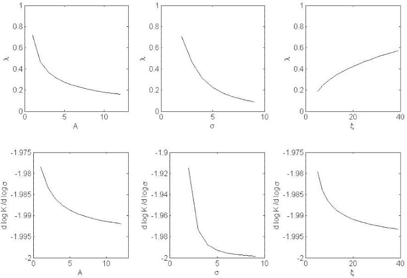
7.1 Model: Solution for Optimal Level of Ownership
For the model in Section II, let
![]() . The optimal choice of insider ownership,
. The optimal choice of insider ownership, ![]() , and
transfers,
, and
transfers, ![]() , solves the following maximization program:
, solves the following maximization program:
subject to ( 5) to ( 7).
7.2.1 Replacement Value of Capital
We follow the methodology of Salinger and Summers (1983) and use the perpetual inventory method to compute the replacement value of the capital stock. We initialize the first value of the capital stock as gross PPE (item 7). We then construct the capital stock iteratively as
![]() , where
, where ![]() is the price
deflator for fixed non residential investment,
is the price
deflator for fixed non residential investment, ![]() is capital expenditure (data128), and
is capital expenditure (data128), and ![]() is book depreciation rate at the three-digit SIC level. We compute
is book depreciation rate at the three-digit SIC level. We compute
![]() , where
, where ![]() is the useful life of capital goods, computed as
is the useful life of capital goods, computed as
![]() .
.
7.2.2 Tobin's
We construct the numerator of ![]() as December market value of equity, plus book value of debt (item 9), plus book value of preferred stock (item 56), minus inventories (item 3). The
denominator is the replacement value of capital.
as December market value of equity, plus book value of debt (item 9), plus book value of preferred stock (item 56), minus inventories (item 3). The
denominator is the replacement value of capital.
7.2.3 Insider Ownership
Our source of managerial ownership data is the Thomson Financial Institutional Holdings database of filings derived from Forms 3, 4, and 5 over the period 1986 to 2005. The measure of insider ownership in year ![]() equals the reported yearly holdings of a firm's shares held by firm officers at the end of that year or at the latest filing date, as a fraction of the shares outstanding in the firm. We include insiders with the following role
classifications: O, OD, OE, OB, OP, OS, OT, OX, CEO, CFO, CI, CO, CT, H, GM, M, MD, P, EVP, VP, and SVP.
equals the reported yearly holdings of a firm's shares held by firm officers at the end of that year or at the latest filing date, as a fraction of the shares outstanding in the firm. We include insiders with the following role
classifications: O, OD, OE, OB, OP, OS, OT, OX, CEO, CFO, CI, CO, CT, H, GM, M, MD, P, EVP, VP, and SVP.
7.2.4 Convexity of Executive Compensation Scheme
We use data on CEO option grants from Execucomp and the Black-Scholes option pricing model as adjusted for dividends by Merton (1973) to compute the partial derivatives with respect to stock return volatility (![]() ) and to stock price (
) and to stock price (![]() ). We use the Core and Guay (2002) procedure for deriving approximate estimates of the time to maturity
and of the exercise price for existing option grants. We construct firm-level measures of convexity and level exposure by aggregating across executives in Execucomp:
). We use the Core and Guay (2002) procedure for deriving approximate estimates of the time to maturity
and of the exercise price for existing option grants. We construct firm-level measures of convexity and level exposure by aggregating across executives in Execucomp:
7.2.5 Option-Adjusted Insider Ownership
Since one single share has ![]() , endowing the manager with
, endowing the manager with ![]() options with
a
options with
a
![]() is equivalent, in terms of stock price exposure, to endowing him with
is equivalent, in terms of stock price exposure, to endowing him with
![]() units of stock. We thus add
units of stock. We thus add
![]() to the number of shares held by insiders.
to the number of shares held by insiders.
7.2.6 Institutional Ownership
We obtain data on institutional holdings from the Thomson Financial (13F) database. We extract quarterly holdings starting in the first quarter of 1980 and ending in the last quarter of 2005. We calculate the share of institutional ownership by summing the stock holdings of all reporting institutions for each stock at the end of each year. We follow Nagel (2005) in adjusting institutional data for stock splits.
7.2.7 Measure of Tobin's from
IBES Data on Analysts' Earnings Forecasts
We follow Cummins, Hassett, and Oliner (2006) in constructing our alternative measure for ![]() , denoted by
, denoted by ![]() , for each firm
, for each firm ![]() and each year
and each year ![]() :
:
![\displaystyle Q^{ibes}=\beta ECF_{it}+\beta^2(1-\delta)ECF_{i,t+1}+\frac{1}{2}(ECF_{i,t}+ECF_{i,t+1})\sum_{k=3}^{n}[\beta^k (1-\delta)^{k-1}(1+EGR_{it})^{k-2}]\;,](img196.gif) |
where
7.2.8 IMC-beta
We use the firm's stock return beta with respect to the IMC portfolio returns as a measure of the firm's investment-specific shock sensitivity. For every firm in Compustat with sufficient stock return data, we estimate a time series of
![]() from the regression
from the regression
Here,
We omit firms with fewer than 40 weekly stock return observations per year, firms in their first three years following the first appearance in Compustat, firms in the investment sector, financial firms (SIC codes 6000-6799), utilities (SIC codes 4900-4949), and government-regulated industries (SIC code >9000).
7.2.9 Customer Concentration
Our measure of customer concentration is based on the Herfindahl index:
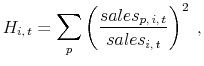 |
where
7.2.10 Age-Adjusted Price Discount between Used and New Capital
We use the data from Ramey and Shapiro (2001). The data consist of used sales prices from auctions of equipment from aerospace plants that closed during the 1990s. The data are at the equipment level, and consist of the sale price of the equipment (S), its original acquisition cost (C), and its
age (A), along with the SIC code of the buyer. We use these data to construct a measure of the age-adjusted discount (from new to used) at the level of the purchasing industry. Our age-adjusted discount measure is the residual ![]() from the regression
from the regression
7.2.11 Purchases of New versus Used Capital Goods
Our data come from the annual capital expenditures survey (ACES), published by the Census Bureau. We use the 1994 survey, Table 2, and compute the ratio of total expenditures to total new expenditures at industry level, using SIC codes.
7.2.12 Credit Rating
Our data on credit ratings come from Standard and Poor's. We use the firm's long-term credit rating (lrating).
7.2.13 Firm Industry Beta
We estimate the firm's sensitivity to its corresponding industry portfolio from equation (9).
7.2.14 Industry Capital Depreciation
We measure capital depreciation as the ratio of item 103 (or item 14 - item 65 if missing) to the replacement value of capital. We compute the average at the three-digit SIC industry level by year.
7.2.15 Industry Capital Sales
We measure capital sales as the ratio of sales of property, plant, and equipment (item 107) to the replacement cost of capital. We compute the industry-level average of capital sales over the first half of the sample (1970 to 1987).
7.2.16 Investment and Volatility during the Financial Crisis
We compute the average investment rate and the lagged idiosyncratic volatility for each portfolio, weighted by lagged capital stock, as follows:
8 References
Abel, Andrew B., 1983, Optimal investment under uncertainty, American Economic Review 73, 228-233.
Admati, Anat R., Paul Pfleiderer, and Josef Zechner, 1994, Large shareholder activism, risk sharing, and financial market equilibrium, Journal of Political Economy 102, 1097-1130.
Angeletos, George-Marios, 2007, Uninsured idiosyncratic investment risk and aggregate saving, Review of Economic Dynamics 10, 1-30.
Arellano, Manuel, and Stephen Bond, 1991, Some tests of specification for panel data: Monte Carlo evidence and an application to employment equations, Review of Economic Studies 58, 277-297.
Bakke, Tor-Erik, and Toni M. Whited, 2010, Which firms follow the market? An analysis of corporate investment decisions, Review of Financial Studies 23, 1941-1980.
Berk, Jonathan B., Richard C. Green, and Vasant Naik, 1999, Optimal investment, growth options, and security returns, Journal of Finance 54, 1553-1607.
Bertrand, Marianne, and Antoinette Schoar, 2003, Managing with style: The effect of managers on firm policies, Quarterly Journal of Economics 118, 1169-1208.
Bloom, Nicholas, 2009, The impact of uncertainty shocks, Econometrica 77, 623-685.
Bloom, Nick, Stephen Bond, and John VanReenen, 2007, Uncertainty and investment dynamics, Review of Economic Studies 74, 391-415.
Bond, Stephen R., and Jason G. Cummins, 2004, Uncertainty and investment: An empirical investigation using data on analysts' profits forecasts, Working paper, Federal Reserve Board.
Bulan, Laarni T., 2005, Real options, irreversible investment and firm uncertainty: New evidence from U.S. firms, Review of Financial Economics 14, 255-279.
Caballero, Ricardo J., 1991, On the sign of the investment-uncertainty relationship, American Economic Review 81, 279-88.
Chen, Hui, Jianjun Miao, and Neng Wang, 2010, Entrepreneurial finance and nondiversifiable risk, Review of Financial Studies 23, 4348-4388.
Core, John, and Wayne Guay, 2002, Estimating the value of employee stock option portfolios and their sensitivities to price and volatility, Journal of Accounting Research 40, 613-630.
Cummins, Jason G., Kevin A. Hassett, and Stephen D. Oliner, 2006, Investment behavior, observable expectations, and internal funds, American Economic Review 96, 796-810.
DeMarzo, Peter, Mike Fishman, Zhiguo He, and Neng Wang, 2010, Dynamic agency and the q theory of investment, Journal of Finance, forthcoming.
Eberly, Janice, Sergio Rebelo, and Nicolas Vincent, 2008, Investment and value: A neoclassical benchmark, NBER Working paper 13866.
Eisfeldt, Andrea, and Dimitris Papanikolaou, 2010, Organization capital and the cross-section of expected returns, Working paper, Kellogg School of Management.
Erickson, Timothy, and Toni M. Whited, 2000, Measurement error and the relationship between investment and Q, Journal of Political Economy 108, 1027-1057.
Erickson, Timothy, and Toni M. Whited, 2002, Two-step GMM estimation of the errors-in-variables model using high-order moments, Econometric Theory 18, 776-799.
Erickson, Timothy, and Toni M. Whited, 2011, Treating measurement error in Tobin’s ![]() , Review of Financial Studies, forthcoming.
, Review of Financial Studies, forthcoming.
Fama, Eugene F., and Kenneth R. French, 1993, Common risk factors in the returns on stocks and bonds, Journal of Financial Economics 33, 3-56.
Fama, Eugene F., and Kenneth R. French, 1997, Industry costs of equity, Journal of Financial Economics 43, 153-193.
Fama, Eugene F., and James D. MacBeth, 1973, Risk, return, and equilibrium: Empirical tests, Journal of Political Economy 81, 607-636.
Fazzari, Steven M., R. Glenn Hubbard, and Bruce C. Petersen, 1988, Financing constraints and corporate investment, Brookings Papers on Economic Activity 19, 141-206.
Froot, Kenneth A., David S. Scharfstein, and Jeremy C. Stein, 1993, Risk management: Coordinating corporate investment and financing policies, Journal of Finance 48, 1629-1658.
Gillan, Stuart L., and Laura T. Starks, 2000, Corporate governance proposals and shareholder activism: The role of institutional investors, Journal of Financial Economics 57, 275-305.
Graham, John R., Campbell R. Harvey, and Manju Puri, 2010, Managerial attitudes and corporate actions, Working paper, Duke University.
Guiso, Luigi, and Giuseppe Parigi, 1999, Investment and demand uncertainty, Quarterly Journal of Economics 114, 185-227.
Hart, Oliver D., 1983, The market mechanism as an incentive scheme, Bell Journal of Economics 14, 366-382.
Hartman, Richard, 1972, The effects of price and cost uncertainty on investment, Journal of Economic Theory 2, 258-266.
Hartzell, Jay C., and Laura T. Starks, 2003, Institutional investors and executive compensation, Journal of Finance 58, 2351-2374.
Himmelberg, Charles P., R. Glenn Hubbard, and Inessa Love, 2002, Investment, protection, ownership, and the cost of capital, Working paper 2834, World Bank.
Holmström, Bengt, 1979, Moral hazard and observability, Bell Journal of Economics 10, 74-91.
Kleibergen, Frank, and Richard Paap, 2006, Generalized reduced rank tests using the singular value decomposition, Journal of Econometrics 133, 97-126.
Knopf, John D., Jouahn Nam, and John H. Thornton, 2002, The volatility and price sensitivities of managerial stock option portfolios and corporate hedging, Journal of Finance 57, 801-813.
Kogan, Leonid, and Dimitris Papanikolaou, 2010a, Growth opportunities and technology shocks, American Economic Review, Papers and Proceedings 100, 532-536.
Kogan, Leonid, and Dimitris Papanikolaou, 2010b, Growth opportunities and technology shocks, Working paper, MIT Sloan School of Management and Kellogg School of Management.
Leahy, John V., and Toni M. Whited, 1996, The effect of uncertainty on investment: Some stylized facts, Journal of Money, Credit and Banking 28, 64-83.
Malmendier, Ulrike, and Geoffrey Tate, 2005, CEO overconfidence and corporate investment, Journal of Finance 60, 2661-2700.
Merton, Robert C., 1973. Theory of Rational Option Pricing, Bell Journal of Economics, 4, 141-183.
Moskowitz, Tobias J., and Annette Vissing-Jørgensen, 2002, The returns to entrepreneurial investment: A private equity premium puzzle? American Economic Review 92, 745-778.
Myers, Stewart C., 1977, Determinants of corporate borrowing, Journal of Financial Economics 5, 147-175.
Nagel, Stefan, 2005, Short sales, institutional investors and the cross-section of stock returns, Journal of Financial Economics 78, 277-309.
Ramey, Valerie A., and Matthew D. Shapiro, 2001, Displaced capital: A study of aerospace plant closings, Journal of Political Economy 109, 958-992.
Roberts, Michael R., and Toni M. Whited, 2011, Endogeneity in empirical corporate finance, Working paper, Wharton School and Simon School of Business.
Ross, Stephen A., 2004, Compensation, incentives, and the duality of risk aversion and riskiness, Journal of Finance 59, 207-225.
Salinger, Michael, and Lawrence H. Summers, 1983, Tax reform and corporate investment: A microeconometric simulation study, in NBER chapters: Behavioral Simulation Methods in Tax Policy Analysis (National Bureau of Economic Research, Inc.).
Shleifer, Andrei, and Robert W. Vishny, 1992, Liquidation values and debt capacity: A market equilibrium approach, Journal of Finance 47, 1343-1366.
Stock, James H., and Motohiro Yogo, 2005, Asymptotic distributions of instrumental variables statistics with many weak instruments, in Donald W. K. Andrews, and James H. Stock, eds.: Identification and Inference for Econometric Models: Essays in Honor of Thomas Rothenberg (Cambridge University Press).
Whited, Toni M., and Guojun Wu, 2006, Financial constraints risk, Review of Financial Studies 19, 531-559.
Table I reports estimation results of equation (11), where the dependent variable is the investment rate (
![]() ). Our baseline measure of risk,
). Our baseline measure of risk,
![]() , is constructed from a regression of weekly firm-level returns on the CRSP VW index and the corresponding industry portfolio. Additional regressors
include lagged values of: Tobin's
, is constructed from a regression of weekly firm-level returns on the CRSP VW index and the corresponding industry portfolio. Additional regressors
include lagged values of: Tobin's ![]() (
(![]() ) defined as in Fazzari, Hubbard, and
Petersen (1988); operating cashflows (
) defined as in Fazzari, Hubbard, and
Petersen (1988); operating cashflows (
![]() ) defined as the ratio of operating income (item 18) to the replacement cost of capital, computed as in Salinger and Summers (1983); the firm's size (
) defined as the ratio of operating income (item 18) to the replacement cost of capital, computed as in Salinger and Summers (1983); the firm's size (
![]() ) defined as the log value of its replacement cost of capital, scaled by average capital across all firms; the firm's stock return (
) defined as the log value of its replacement cost of capital, scaled by average capital across all firms; the firm's stock return (![]() ); leverage (
); leverage (
![]() ) defined as the ratio of book equity (item 216) to book assets (item 6); and systematic volatility (
) defined as the ratio of book equity (item 216) to book assets (item 6); and systematic volatility (
![]() ) defined as the (log of the) square root of the difference between the firm's total variance and its idiosyncratic variance. Item refers to Compustat items. The sample period is 1970 to 2005. Here,
) defined as the (log of the) square root of the difference between the firm's total variance and its idiosyncratic variance. Item refers to Compustat items. The sample period is 1970 to 2005. Here, ![]() denotes firm fixed effects,
denotes firm fixed effects, ![]() denotes time fixed effects, and
denotes time fixed effects, and ![]() denotes industry-time fixed effects. The standard errors are clustered at the firm-level, and
denotes industry-time fixed effects. The standard errors are clustered at the firm-level, and ![]() -statistics are reported in parentheses.
-statistics are reported in parentheses.
|
|
No Controls | BENCH |
|
Syst |
|
|
-0.0346(-13.78) | -0.0196(-8.44) | -0.0197(-8.32) | -0.0244(-9.94) |
|
|
0.0063(5.51) | |||
|
|
0.069(45.05) | 0.0692(43.41) | 0.0690(44.31) | |
|
|
0.0222(9.91) | 0.0218(9.88) | 0.0220(9.84) | |
|
|
-0.1179(-31.80) | -0.1243(-31.67) | -0.1188(-32.09) | |
| 0.0146(8.66) | 0.0131(7.47) | 0.0148(8.75) | ||
|
|
0.0352(14.13) | 0.0346(13.82) | 0.0346(13.96) | |
| Observations | 104646 | 104646 | 104646 | 104619 |
| 0.399 | 0.563 | 0.569 | 0.563 | |
| Fixed effects | F | F,T | F, |
F, T |
| Estimation Method | OLS | OLS | OLS | OLS |
| Level of insider ownership | Low | 2 | 3 | 4 | High |
| Insider ownership | 0.06 | 0.32 | 1.01 | 3.40 | 17.43 |
| Market capitalization (scaled by mean) | 20.84 | 17.23 | 11.01 | 6.61 | 3.51 |
| Book assets (scaled by mean) | 27.38 | 21.04 | 13.13 | 7.44 | 4.38 |
| Tobin's |
1.64 | 1.80 | 1.93 | 2.27 | 2.15 |
| Cashflows to capital | 12.27 | 14.41 | 15.17 | 15.98 | 16.05 |
| Investment to capital | 8.76 | 9.41 | 10.57 | 12.18 | 12.47 |
| Idiosyncratic volatility | 35.37 | 36.65 | 40.74 | 44.62 | 49.11 |
| Physical capital to book assets | 63.47 | 58.13 | 54.11 | 47.36 | 46.61 |
| Whited-Wu index | -29.77 | -28.65 | -25.99 | -23.02 | -19.71 |
| Book debt to book assets | 21.96 | 20.92 | 19.39 | 17.29 | 16.88 |
| Cash to book assets | 6.58 | 6.64 | 7.47 | 8.71 | 8.38 |
| Dividends to cashflows | 3.69 | 2.14 | 0.74 | 0.00 | 0.00 |
| Sales / industry sales | 1.75 | 1.32 | 0.88 | 0.46 | 0.31 |
Table III reports estimation results of equation (11), interacting our idiosyncratic volatility measure (
![]() ) with insider ownership quintile dummies (see Appendix for details). Here,
) with insider ownership quintile dummies (see Appendix for details). Here, ![]() and
and ![]() indicate the dummies for the first and the fifth insider ownership quintile, respectively. The third and fourth columns adjust insider ownership for option
holdings, whenever available, otherwise option holdings are assumed to be zero. Depending on the specification, we include firm (
indicate the dummies for the first and the fifth insider ownership quintile, respectively. The third and fourth columns adjust insider ownership for option
holdings, whenever available, otherwise option holdings are assumed to be zero. Depending on the specification, we include firm (![]() ) and year (
) and year (![]() ) fixed effects. The set of controls includes Tobin's
) fixed effects. The set of controls includes Tobin's ![]() , operating cashflows, firm size, the firm's stock return, and leverage
(see notes to Table I for details). We interact time and firm fixed effects with quintile dummies. The standard errors are clustered at the firm level, and
, operating cashflows, firm size, the firm's stock return, and leverage
(see notes to Table I for details). We interact time and firm fixed effects with quintile dummies. The standard errors are clustered at the firm level, and ![]() -statistics are reported in
parentheses.
-statistics are reported in
parentheses.
|
|
(1) | (2) | (3) | (4) |
|
|
-0.0089(-1.10) | -0.0049(-0.62) | -0.0012(-0.12) | -0.0046(-0.51) |
|
|
-0.0155(-2.02) | -0.0045(-0.62) | -0.0086(-0.95) | -0.0019(-0.22) |
|
|
-0.0245(-2.90) | -0.0070(-0.83) | -0.0201(-1.95) | -0.0109(-1.06) |
|
|
-0.0400(-4.13) | -0.0161(-1.72) | -0.0312(-2.61) | -0.0190(-1.65) |
|
|
-0.0413(-3.52) | -0.0305(-2.93) | -0.0408(-2.81) | -0.0331(-2.60) |
|
|
-0.0324 | -0.0255 | -0.0396 | -0.0285 |
| p-value | 0.022 | 0.049 | 0.023 | 0.066 |
| Observations | 41206 | 41206 | 32616 | 32616 |
| Fixed effects | F | F, T | F | F, T |
| Controls | N | Y | N | Y |
| Option-adjusted ownership | N | N | Y | Y |
Table IV reports estimation results of equation (11) separately for firms with different levels of insider ownership and convexity of executive compensation. See Appendix for details on the construction of our compensation convexity and insider ownership measures.
Every year, we first sort firms into terciles based on ownership by insiders (High, Medium, Low) and then sort into terciles based on the sensitivity of compensation to volatility (High, Medium, Low). We report results for the four corner portfolios. The sample period is 1992 to 2005. Depending on
the specification, we include firm (![]() ) and year (
) and year (![]() ) fixed effects. The set of
controls includes Tobin's
) fixed effects. The set of
controls includes Tobin's ![]() , operating cashflows, firm size, the firm's stock return, and leverage (see notes to Table I for details). We interact time and firm fixed effects with quintile
dummies. The standard errors are clustered at the firm level, and
, operating cashflows, firm size, the firm's stock return, and leverage (see notes to Table I for details). We interact time and firm fixed effects with quintile
dummies. The standard errors are clustered at the firm level, and ![]() -statistics are reported in parentheses. We report the Chow test p-value for the null hypothesis
that the idiosyncratic volatility,
-statistics are reported in parentheses. We report the Chow test p-value for the null hypothesis
that the idiosyncratic volatility,
![]() , coefficients on the high and low vega groups are the same.
, coefficients on the high and low vega groups are the same.
| I/K | (1) | (2) | (3) | (4) |
|
|
-0.0221(-2.10) | -0.0172(-1.87) | -0.0223(-2.10) | -0.0175(-1.90) |
|
|
0.0112(1.72) | 0.0127(1.79) | 0.0112(1.73) | 0.0108(1.57) |
|
|
0.0333 | 0.0299 | 0.0335 | 0.0283 |
| p-value | 0.007 | 0.009 | 0.007 | 0.013 |
|
|
-0.0315(-2.79) | -0.0286(-2.83) | -0.0320(-2.81) | -0.0296(-2.91) |
|
|
0.0152(1.32) | -0.0001(-0.01) | 0.0148(1.28) | -0.0007(-0.07) |
|
|
0.0467 | 0.0285 | 0.0468 | 0.0289 |
| p-value | 0.004 | 0.054 | 0.004 | 0.052 |
| Total observations | 12708 | 12708 | 12708 | 12708 |
| Fixed effects | F | F, T | F | F, T |
| Controls | N | Y | N | Y |
| Option-adjusted ownership | N | N | Y | Y |
| I/K | (1) | (2) | (3) | (4) |
|
|
-0.0110(-1.12) | 0.0042(0.45) | -0.0116(-1.03) | 0.0050(0.45) |
|
|
-0.0627(-5.21) | -0.0359(-3.40) | -0.0740(-5.04) | -0.0453(-3.68) |
|
|
-0.0517 | -0.0401 | -0.0624 | -0.0503 |
| p-value | 0.001 | 0.004 | 0.001 | 0.002 |
|
|
-0.0077(-1.34) | 0.0005(0.08) | 0.0005(0.08) | -0.0009(-0.11) |
|
|
-0.0098(-0.97) | 0.0041(0.38) | 0.0047(0.41) | 0.0001(0.00) |
|
|
-0.0021 | 0.0036 | 0.0042 | 0.0010 |
| p-value | 0.857 | 0.775 | 0.752 | 0.952 |
| Total observations | 40705 | 40705 | 32230 | 32230 |
| Fixed effects | F | F, T | F | F, T |
| Controls | N | Y | N | Y |
| Option-adjusted ownership | N | N | Y | Y |
Table VI reports estimation results of a modified version of equation (11), where the dependent variable is the investment rate (
![]() ). Here,
). Here, ![]() is constructed from analysts' forecasts as in
Cummins, Hassett, and Oliner (2006). Next,
is constructed from analysts' forecasts as in
Cummins, Hassett, and Oliner (2006). Next,
![]() refers to the firm's univariate beta with a portfolio long the capital-producing sector and short the consumption-producing sector (IMC); see Kogan and Papanikolaou (2010a,
2010b) for more details. In columns 1 to 3 the set of additional controls includes operating cashflows, firm size, the firm's stock return, and leverage (see notes to Table I for details). In columns 4 and 5 we include the lagged investment rate and we replace firm size with the firm's total sales
(scaled by industry sales at the three-digit SIC level) as controls. Depending on the specification, we include firm (
refers to the firm's univariate beta with a portfolio long the capital-producing sector and short the consumption-producing sector (IMC); see Kogan and Papanikolaou (2010a,
2010b) for more details. In columns 1 to 3 the set of additional controls includes operating cashflows, firm size, the firm's stock return, and leverage (see notes to Table I for details). In columns 4 and 5 we include the lagged investment rate and we replace firm size with the firm's total sales
(scaled by industry sales at the three-digit SIC level) as controls. Depending on the specification, we include firm (![]() ), industry (
), industry (![]() ), and/or year (
), and/or year (![]() ) fixed effects. Column 5 presents results using the Erickson and Whited (2000) estimator. We report the p-value of a joint test for the null of no identification across all time periods using the Bonferroni method and the
) fixed effects. Column 5 presents results using the Erickson and Whited (2000) estimator. We report the p-value of a joint test for the null of no identification across all time periods using the Bonferroni method and the ![]() statistic. Columns 6 and 7 present estimation
results using instrumental variables, where we instrument for idiosyncratic risk (
statistic. Columns 6 and 7 present estimation
results using instrumental variables, where we instrument for idiosyncratic risk (
![]() ) with the concentration of a firm's customer base,
) with the concentration of a firm's customer base, ![]() ,
constructed using customer data from the Compustat segment files (see text for details). We report the value of the Kleibergen-Paap rk Wald F-test of the null of weak instruments. The critical value assuming 10% maximal IV size equals 16.38
(Stock and Yogo (2005)). In columns 1 to 3 and 6 to 7, standard errors are clustered at the firm level. In columns 4 and 5, standard errors are computed using the Fama and Mcbeth (1973) procedure.
,
constructed using customer data from the Compustat segment files (see text for details). We report the value of the Kleibergen-Paap rk Wald F-test of the null of weak instruments. The critical value assuming 10% maximal IV size equals 16.38
(Stock and Yogo (2005)). In columns 1 to 3 and 6 to 7, standard errors are clustered at the firm level. In columns 4 and 5, standard errors are computed using the Fama and Mcbeth (1973) procedure.
|
|
|
|
OLS | IV | |||
|
|
-0.0175(-4.78) | -0.0464(-15.60) | -0.0090(-2.09) | -0.0366(-11.95) | -0.0323(-6.18) | -0.1167(-7.00) | -0.1483(-6.88) |
|
|
0.0435(16.83) | 0.0248(6.00) | |||||
|
|
0.0074(7.58) | 0.0016(0.93) | |||||
| 0.0032(9.48) | 0.0079(2.20) | ||||||
|
|
0.0512(14.81) | 0.0569(45.48) | |||||
| Observations | 33628 | 77001 | 24904 | 104646 | 104646 | 91157 | 91157 |
| Bonferroni test (p-value) | 0.001 | ||||||
| 0.465 | |||||||
| Kleibergen-Paap rk Wald F statistic | 299.3 | 230.7 | |||||
| Fixed effects | F,T | F,T | F,T | F,T | F,T | I | I,T |
| Controls | Y | Y | Y | Y | Y | Y | Y |
| Estimation method | OLS | OLS | OLS | OLS | GMM | IV | IV |
| I/K | (1) | (2) | (3) | (4) | (5) | (6) |
|
|
-0.0070(-0.77) | 0.0050(0.57) | -0.0046(-0.47) | -0.0009(-0.11) | -0.0055(-0.61) | 0.0035(0.40) |
|
|
-0.0179(-1.94) | -0.0091(-1.03) | -0.0199(-2.24) | -0.0111(-1.31) | -0.0242(-2.41) | -0.0140(-1.54) |
|
|
-0.0237(-2.29) | -0.0146(-1.55) | -0.0185(-1.79) | -0.0073(-0.71) | -0.0286(-2.83) | -0.0170(-1.85) |
|
|
-0.0372(-3.98) | -0.0028(-0.31) | -0.0353(-3.78) | -0.0148(-1.61) | -0.0412(-4.36) | -0.0123(-1.28) |
|
|
-0.0285(-2.53) | -0.0275(-2.66) | -0.0322(-3.05) | -0.0241(-2.49) | -0.0311(-2.70) | -0.0280(-2.63) |
|
|
-0.0215 | -0.0325 | -0.0277 | -0.0232 | -0.0256 | -0.0315 |
| p-value | 0.059 | 0.002 | 0.014 | 0.023 | 0.026 | 0.004 |
| Observations | 40985 | 40985 | 40773 | 40773 | 41206 | 41206 |
| Financial constraints | WW | WW | RT | RT | A | A |
| Fixed effects | F | F, T | F | F, T | F | F, T |
| Controls | N | Y | N | Y | N | Y |
|
|
(1) | (2) | (3) | (4) | (5) | (6) | (7) | (8) | (9) | (10) |
|
|
0.0024(0.10) | 0.0226(0.90) | -0.0127(-1.91) | -0.0044(-0.72) | -0.0126(-2.02) | -0.0012(-0.20) | -0.0134(-2.23) | -0.0043(-0.72) | -0.0129(-2.06) | -0.0036(-0.58) |
|
|
-0.0231(-0.75) | -0.0098(-0.27) | -0.0256(-3.94) | -0.0134(-2.09) | -0.0259(-3.92) | -0.0114(-1.68) | -0.0276(-4.19) | -0.0140(-2.07) | -0.0219(-3.17) | -0.0083(-1.28) |
|
|
-0.0816(-2.32) | -0.0648(-1.94) | -0.0377(-4.89) | -0.0214(-3.03) | -0.0338(-4.41) | -0.0206(-2.96) | -0.0407(-5.31) | -0.0258(-3.72) | -0.0454(-6.11) | -0.0297(-4.34) |
|
|
-0.0840 | -0.0874 | -0.0250 | -0.0171 | -0.0212 | -0.0194 | -0.0273 | -0.0215 | -0.0325 | -0.0261 |
| p-value | 0.048 | 0.036 | 0.013 | 0.062 | 0.028 | 0.033 | 0.004 | 0.015 | 0.001 | 0.004 |
| Observations | 2184 | 2184 | 41179 | 41179 | 40454 | 40454 | 40661 | 40661 | 40828 | 40828 |
|
|
(1) | (2) | (3) | (4) | (5) | (6) | (7) | (8) | (9) | (10) |
|
|
0.0239(1.15) | 0.0291(1.53) | -0.0093(-1.67) | -0.0018(-0.34) | -0.0074(-1.27) | 0.0012(0.21) | -0.0124(-2.26) | -0.0007(-0.14) | -0.0091(-1.56) | 0.0001(0.03) |
|
|
-0.0481(-1.42) | -0.0047(-0.13) | -0.0281(-4.26) | -0.0100(-1.59) | -0.0281(-4.45) | -0.0076(-1.19) | -0.0335(-5.17) | -0.0130(-1.93) | -0.0284(-4.33) | -0.0105(-1.66) |
|
|
-0.0630(-1.74) | -0.0536(-1.45) | -0.0438(-5.46) | -0.0275(-3.59) | -0.0404(-4.97) | -0.0255(-3.36) | -0.0417(-5.10) | -0.0274(-3.64) | -0.0442(-5.47) | -0.0293(-3.91) |
|
|
-0.0868 | -0.0827 | -0.0345 | -0.0257 | -0.0331 | -0.0267 | -0.0293 | -0.0266 | -0.0352 | -0.0295 |
| p-value | 0.046 | 0.046 | 0.000 | 0.005 | 0.001 | 0.005 | 0.003 | 0.004 | 0.000 | 0.001 |
| Observations | 2184 | 2184 | 41028 | 41028 | 40308 | 40308 | 40517 | 40517 | 40682 | 40682 |
| Irreversibility measure | P | P |
|
|
U | U | S | S | ||
| Fixed effects | F | F, T | F | F, T | F | F, T | F | F, T | F | F, T |
| Controls | N | Y | N | Y | N | Y | N | Y | N | Y |
| A: Change in log idiosyncratic volatility (relative to 2006) for firms with high (solid line) and low (dotted line) insider ownership | B: Change in portfolio investment rates (relative to 2006) for firms with high (solid line) and low (dotted line) insider ownership firms |
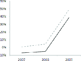 Figure 1a Data |
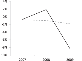 Figure 1b Data |
| C: Change in portfolio investment rates (relative to 2006) for firms with high (solid line) and low (dotted line) compensation convexity | D: Change in portfolio investment rates (relative to 2006) for firms with high (solid line) and low (dotted line) insider ownership, conditional on high (grey line) or low (black line) institutional ownership. |
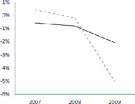 Figure 1c Data |
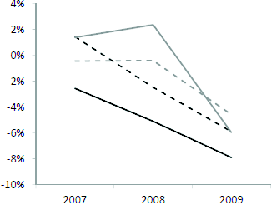 Figure 1d Data |
| E: Black line is difference in average (weighted by capital stock) portfolio investment rates between high and low insider ownership firms (right axis); grey line is average (weighted by capital stock) idiosyncratic volatility across firms (left axis). | F: Black line is difference in median portfolio investment rates between high and low insider ownership firms (right axis); grey line is median idiosyncratic volatility across firms (left axis). |
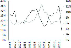 Figure 1e Data |
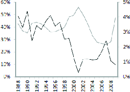 Figure 1f Data |
Footnotes
 . Note that systematic volatility varies in the cross-section due to cross-sectional dispersion in
betas with the market and industry portfolios. Return to Text
. Note that systematic volatility varies in the cross-section due to cross-sectional dispersion in
betas with the market and industry portfolios. Return to Text